Sparsity-promoting algorithms for the discovery of informative Koopman-invariant subspaces

Abstract

Koopman decomposition is a non-linear generalization of eigen-decomposition, and is being increasingly utilized in the analysis of spatio-temporal dynamics. Well-known techniques such as the dynamic mode decomposition (DMD) and its linear variants provide approximations to the Koopman operator, and have been applied extensively in many fluid dynamic problems. Despite being endowed with a richer dictionary of nonlinear observables, nonlinear variants of the DMD, such as extended/kernel dynamic mode decomposition (EDMD/KDMD) are seldom applied to large-scale problems primarily due to the difficulty of discerning the Koopman invariant subspace from thousands of resulting Koopman eigenmodes. To address this issue, we propose a framework based on multi-task feature learning to extract the most informative Koopman invariant subspace by removing redundant and spurious Koopman triplets. In particular, we develop a pruning procedure that penalizes departure from linear evolution. These algorithms can be viewed as sparsity promoting extensions of EDMD/KDMD. Further, we extend KDMD to a continuous-time setting and show a relationship between the present algorithm, sparsity-promoting DMD, and an empirical criterion from the viewpoint of non-convex optimization. The effectiveness of our algorithm is demonstrated on examples ranging from simple dynamical systems to two-dimensional cylinder wake flows at different Reynolds numbers and a three-dimensional turbulent ship air-wake flow. The latter two problems are designed such that very strong nonlinear transients are present, thus requiring an accurate approximation of the Koopman operator. Underlying physical mechanisms are analyzed, with an emphasis on characterizing transient dynamics. The results are compared to existing theoretical expositions and numerical approximations.

1 Introduction

Complex unsteady flow phenomena such as turbulence (Pope, 2001), flow instability (Drazin & Reid, 2004; Lietz et al., 2017), and fluid-structure interactions (Dowell & Hall, 2001) are prevalent in many physical systems. To analyze and understand such phenomena, it is useful to extract coherent modes associated with important dynamical mechanisms and track their evolution. Koopman operator theory (Budišić et al., 2012) offers an elegant framework to reduce spatio-temporal fields associated with non-linear dynamics as a linear combination of time evolving modes ordered by frequency and growth rates (Rowley et al., 2009).

Consider a general continuous nonlinear dynamical system $\dot{\mathbf{x}}=\mathbf{F}(\mathbf{x})$, where the system state $\mathbf{x}$ evolves on a manifold $\mathcal{M}\subset\mathbb{R}^{N}$. $\mathbf{F}:\mathcal{M}\mapsto T\mathcal{M}$ is a vector-valued smooth function and $T\mathcal{M}$ is the tangent bundle, i.e., $\forall p\in\mathcal{M},\mathbf{F}(p)\in T_{p}\mathcal{M}$. The aforementioned task of decomposition is equivalent to finding a set of $L$ observables associated with the system, $\{g_{i}\}_{i=1}^{L}$ $(g_{i}:\mathcal{M}\mapsto\mathbb{C})$, that evolve linearly in time while spanning the system state $\mathbf{x}$. The significance of the above statement is that it represents a global linearization of the nonlinear dynamical system (Budišić et al., 2012; Brunton et al., 2016a).

Formally, this idea can be traced back to Koopman operator theory for Hamiltonian dynamical systems introduced by Koopman (1931) to study the evolution of observables $g$ on $L^{2}(\mathcal{M})$, which is a vector space of square integrable functions defined on the manifold $\mathcal{M}$. More generally, for a certain vector space of observable functions $\mathcal{F}$ defined on the manifold $\mathcal{M}$ and $t>0$, the Koopman semigroup (parameterized by $t$) is the set $\{\mathcal{K}_{t}\}_{t\in\mathbb{R}^{+}}$: $\mathcal{K}_{t}:\mathcal{F}\mapsto\mathcal{F}$ that governs the dynamics of observables in the form $\mathcal{K}_{t}g(\mathbf{x}(0))\triangleq{\color[rgb]{0,0,0}g}(S(t,\mathbf{x}_{0}))=g(\mathbf{x}(t))$ where $S(t,\cdot)$ is the flow map of the dynamical system (Mezić, 2013). $\mathcal{K}=\lim_{t\rightarrow 0}(\mathcal{K}_{t}f-f)/t$ is referred to as the continuous-time Koopman operator, i.e., Koopman generator. While the Koopman operator is linear over the space of observables, $\mathcal{F}$ is most often infinite-dimensional, e.g., $L^{2}(\mathcal{M})$, which makes the approximation of the Koopman operator a difficult problem. Throughout this work, we assume $\mathcal{F}=L^{2}(\mathcal{M})$. Readers interested in a detailed discussion of the choice of $\mathcal{F}$ are referred to Bruce et al. (2019).

A special subspace of $\mathcal{F}$, referred to as a minimal Koopman-invariant subspace $\mathcal{G}$, has the following property: for any $\phi\in\mathcal{G}$, for any $t\in\mathbb{R}^{+}$, $\mathcal{K}_{t}\phi\in\mathcal{G}$ and $\mathbf{x}\in\mathcal{G}$. Existing techniques such as the extended dynamic mode decomposition (Williams et al., 2015) are capable of approximating Koopman operators, but typically yield high dimensional spaces ($L$-dimensional space in fig. 1). In this work, we are interested in accurately approximating such a subspace - but with the minimal possible dimension and Koopman invariance - using learning techniques, as illustrated in fig. 1. This can yield useful coordinates for a multitude of applications including modal analysis and control (Arbabi et al., 2018).

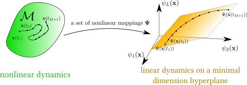
Figure 1: Schematic of transformation of a non-linear system to a linear $L$-dimensional space and the extraction of a minimal Koopman-invariant subspace.

In general, physical systems governed by PDEs, e.g., fluid dynamics, are infinite-dimensional. From a numerical viewpoint, the number of degrees of freedom can be related to the spatial discretization (for example, the number of grid points). Although a finite-dimensional manifold can be extracted (Holmes et al., 2012), e.g., $O(10)$-$O(10^{3})$ dimensions via Proper Orthogonal Decomposition (POD), finding a Koopman-invariant subspace on such manifolds is still challenging. Currently, the most popular method to approximate the Koopman operator is the dynamic mode decomposition (DMD) (Schmid, 2010; Rowley & Dawson, 2017) mainly for two reasons. First, it is straightforward and computationally efficient compared to nonlinear counterparts such as Extended DMD (EDMD) (Williams et al., 2015) and Kernel DMD (KDMD) (Williams et al., 2014). Second, the essence of DMD is to decompose a spatio-temporal field into several temporally growing/decaying travelling/stationary harmonic waves, which are prevalent in fluid mechanics. However, the accuracy of DMD is limited by the assumption that the Koopman-invariant subspace lies in the space spanned by snapshots of the state $\mathbf{x}$. Thus, DMD is used to mainly identify and visualize coherent structures. Indeed, DMD can be interpreted as a $L^{2}$ projection of the action of the Koopman operator on the linear space spanned by snapshots of the system state (Korda & Mezić, 2018b).

To overcome the above limitations, it is natural to augment the observable space with either the history of the state (Arbabi & Mezić, 2017a; Brunton et al., 2017; Kamb et al., 2018; Le Clainche & Vega, 2017) or nonlinear observables of the state (Williams et al., 2014, 2015). Time-delay embedding can be very useful in reduced order modeling of systems for which sparse measurements can be easily obtained, assuming the inputs and outputs are not high dimensional (Korda & Mezić, 2018a). Although time-delay embedding is simple to implement and has strong connections to Takens’ embedding (Kamb et al., 2018; Pan & Duraisamy, 2019), the main practical issue arises in reduced order modeling of high fidelity simulations in a predictive setting due to the requirement of a large number of snapshots of the full order model. Further, if one is only interested in the post-transient dynamics of the system state on an attractor, linear observables with time delays are sufficient to extract an informative Koopman-invariant subspace (Arbabi & Mezić, 2017a; Pan & Duraisamy, 2019; Brunton et al., 2017; Arbabi & Mezić, 2017b; Mezić, 2005; Röjsel, 2017). However, if one is interested in the strongly nonlinear transient dynamics leading to an attractor or reduced order modeling for high fidelity numerical simulations (Xu & Duraisamy, 2019; Xu et al., 2020; Huang et al., 2018; Parish et al., 2020; Carlberg et al., 2013), time-delay embedding may become less appropriate as several delay snapshots of the full order model are required to initialize the model. In that case, nonlinear observables may be more appropriate.

Driven by the interest in modal analysis and control of transient flow phenomena, we consider augmentation of the observable space with nonlinear functions of the state, e.g., EDMD (Williams et al., 2015)/KDMD (Williams et al., 2014). Although it has been reported that KDMD allows for a set of more interpretable Koopman eigenvalues (Williams et al., 2014) and better accuracy (Röjsel, 2017), issues such as mode selection, spurious modes (Kaiser et al., 2017; Zhang et al., 2017), and choice of dictionary/kernel in EDMD/KDMD remain open. In fact, the choice of kernel type and hyperparameter can significantly affect the resulting eigenmodes, distribution of eigenvalues (Kutz et al., 2016), and the accuracy of predictions (Zhang et al., 2017).

Searching for an accurate and informative Koopman-invariant subspace has long been a pursuit in the DMD community. Rowley et al. (2009) and Schmid et al. (2012) considered selecting dominant DMD modes in order of their amplitudes. However, following such a criterion (Tu et al., 2013; Kou & Zhang, 2017), may result in the selection of irrelevant modes that may have large amplitudes, but decay rapidly. As a result, Tu et al. (2013) considered weighting the loss term by the magnitude of eigenvalues to penalize the retention of fast decaying modes. Sparsity-promoting DMD (referred as “spDMD” throughout the paper) developed by Jovanović et al. (2014) recasts mode selection in DMD as an optimization problem with a $\ell_{1}$ penalty. With a preference of stable modes over fast decaying ones, Tissot et al. (2014) proposed a simpler criterion based on time-averaged-eigenvalue-weighted amplitude. This was followed by Kou & Zhang (2017) who used a similar criterion but computed the “energy” of each mode, yielding similar performance to spDMD at a lower computational cost. Based on the orthonormal property of pseudo-inverse, Hua et al. (2017) proposed an ordering of Koopman modes by defining a new “energy”. Compared with previous empirical criteria, the “energy” for each mode involves a pseudo-inverse which combines the influence from all eigenmodes, and therefore the contribution from each mode cannot be isolated. Instead of selecting modes from a “reconstruction” perspective, Zhang et al. (2017) studied the issue of spurious modes by evaluating the deviation of the identified eigenfunctions from linear evolution in an a priori sense. Further, Optimized DMD (Chen et al., 2012; Askham & Kutz, 2018) combines DMD with mode selection simultaneously, which is the forerunner of recently proposed neural network-based models for Koopman eigenfunctions in spirit (Takeishi et al., 2017; Lusch et al., 2018; Otto & Rowley, 2019; Pan & Duraisamy, 2020; Li et al., 2017; Yeung et al., 2019). Regardless of the above issues related to non-convex optimization (Dawson et al., 2016), extension of optimized DMD to EDMD/KDMD is not straightforward. Further, neural network-based models require large amounts of data, are prone to local minima, and lack interpetability. There have been a few attempts towards mode selection in EDMD/KDMD. Brunton et al. (2016a) present an iterative method that augments the dictionary of EDMD until a convergence criterion is reached for the subspace. This is effectively a recursive implementation of EDMD. Recently, Haseli & Cortés (2019) showed that given a sufficient amount of data, if there is any accurate Koopman eigenfunction spanned by the dictionary, it must correspond to one of the obtained eigenvectors. Moreover, they proposed the idea of mode selection by checking if the reciprocal of identified eigenvalue also appears when the temporal sequence of data is reversed, which is similar to the idea of comparing eigenvalues on the complex plane from different trajectories, as proposed by Hua et al. (2017). In contrast to the “bottom-up” method of Brunton et al. (2016a) with subspace augmentation, Hua et al. (2017) proposed a “top-down” subspace subtraction method relying on iteratively projecting the features onto the null space. A similar idea can be traced back to Kaiser et al. (2017) who propose a search for the sparsest vector in the null space.

As the main contribution of this work, we propose a novel EDMD/KDMD framework equipped with the following strategy to extract an accurate yet minimal Koopman-invariant subspace:

1. We first evaluate the normalized maximal deviation of the evolution of each eigenfunction from linear evolution in a posteriori fashion.

2. Using the above criteria, we select a user-defined number of accurate EDMD/KDMD modes;

3. Among the accurate EDMD/KDMD modes obtained above, informative modes are selected using multi-task feature learning (Argyriou et al., 2008a; Bach et al., 2012).

To the best of our knowledge, this is the first model-agnostic attempt to address sparse identification of an accurate minimal Koopman-invariant subspace. Our contribution also extends the classical sparsity-promoting DMD (Jovanović et al., 2014) in a more general setting that includes EDMD/KDMD. The applications are focused on strongly transient flows, and new classes of stable Koopman modes are identified.

The organization of the paper is as follows: In Section 2, we provide a review of EDMD/KDMD in discrete-time and present corresponding extensions to continuous-time. Following this, we discuss current challenges in standard EDMD/KDMD. In Section 3, we propose the framework of sparse identification of informative Koopman-invariant subspaces for EDMD/KDMD with hyperparameter selection and provide implementation details. A novel optimization procedure that penalizes departure from linear evolution is detailed in Sections 3.1 and 3.2. Differences and connections between spDMD, Kou’s emprical criterion, and our proposed framework is shown from the viewpoint of optimization. In Section 4, numerical verification and modal analysis on examples from a fixed point attractor to a transient cylinder wake flow, and a transient ship-airwake are provided. In Section 5, conclusions are drawn.

2 Review of EDMD/KDMD

In this section, we provide a summary of our framework to extract the Koopman operator using EDMD/KDMD in both discrete-time and continuous-time. Although the original EDMD is seldom used for data-driven Koopman analysis in fluid flows due to its poor scaling, it has recently been reported that a scalable version of EDMD can be applied to high-dimensional systems (DeGennaro & Urban, 2019). Since our algorithm to extract the Koopman-invariant subspace is agnostic to the type of technique to compute the original set of Koopman modes, we include both EDMD and KDMD for completeness.

2.1 Extended Dynamic Mode Decomposition

2.1.1 Discrete-time Formulation

For simplicity, consider $M$ sequential snapshots sampled uniformly in time with $\Delta t$ on a trajectory, $\{\mathbf{x}_{i}\}_{i=1}^{M}$. The EDMD algorithm (Williams et al., 2015) assumes a dictionary of $L$ linearly independent functions $i=1,\ldots,L$, $\psi_{i}(\mathbf{x}):\mathcal{M}\mapsto\mathbb{C}$ that approximately spans a Koopman-invariant subspace $\mathcal{F}_{L}$

$$\mathcal{F}_{L}=\textrm{span}\{\psi_{1}(\mathbf{x}),\ldots,\psi_{L}(\mathbf{x})\}.$$ (1)

Thus we can write for any $g\in\mathcal{F}_{L}$ as $g(\mathbf{x})=\mathbf{\Psi}(\mathbf{x})\mathbf{a}$ with $\mathbf{a}\in\mathbb{C}^{L}$, where the feature vector $\mathbf{\Psi}(\mathbf{x})$ is

$$\mathbf{\Psi}(\mathbf{x})=\begin{bmatrix}\psi_{1}(\mathbf{x})&\ldots&\psi_{L}(\mathbf{x})\end{bmatrix}.$$ (2)

Consider a set of $L^{{}^{\prime}}$ observables as $\{g_{l}\}_{l=1}^{L^{{}^{\prime}}}=\{\mathbf{\Psi}\mathbf{a}_{l}\}_{l=1}^{L^{{}^{\prime}}}$, where $\mathbf{a}_{l}\in\mathbb{C}^{L}$ is arbitrary. After the discrete-time Koopman operator $\mathcal{K}_{\Delta t}$ is applied on each $g_{l}$, given data $\{\mathbf{x}_{i}\}_{i=1}^{M}$, we have the following for $l=1,\ldots,L^{\prime}$, and $i=1,\ldots,M-1$,

$$\mathcal{K}_{\Delta t}g_{l}(\mathbf{x}_{i})=g_{l}(\mathbf{x}_{i+1})=\mathbf{\Psi}(\mathbf{x}_{i+1})\mathbf{a}_{l}=\mathbf{\Psi}(\mathbf{x}_{i})\mathbf{K}\mathbf{a}_{l}+r_{i,l},$$ (3)

where $r_{i,l}$ is simply the residual for the $l$-th function on the $i$-th data point. The standard EDMD algorithm seeks a constant matrix $\mathbf{K}\in\mathbb{C}^{L\times L}$ that governs the linear dynamics in the observable space such that the sum of the square of the residuals $r_{i,l}$ from eq. 3 over all samples and functions,

$${}J(\mathbf{K},\{\mathbf{a}_{l}\}_{l=1}^{L^{{}^{\prime}}})=\sum_{l=1}^{L^{{}^{\prime}}}\sum_{m=1}^{M-1}|(\mathbf{\Psi}(\mathbf{x}_{m+1})-\mathbf{\Psi}(\mathbf{x}_{m})\mathbf{K})\mathbf{a}_{l}|^{2}=\lVert(\mathbf{\Psi}_{\mathbf{x}^{{}^{\prime}}}-\mathbf{\Psi}_{\mathbf{x}}\mathbf{K})\mathbf{A}^{{}^{\prime}}\rVert^{2}_{F},$$ (4)

is minimized over $\{\mathbf{x}_{i}\}_{i=1}^{M+1}$. In the above equation,

$$\mathbf{\Psi}_{\mathbf{x}}=\begin{bmatrix}\psi_{1}(\mathbf{x}_{1})&\ldots&\psi_{L}(\mathbf{x}_{1})\\ \vdots&\vdots&\vdots\\ \psi_{1}(\mathbf{x}_{M-1})&\ldots&\psi_{L}(\mathbf{x}_{M-1})\end{bmatrix},\mathbf{\Psi}_{\mathbf{x}^{{}^{\prime}}}=\begin{bmatrix}\psi_{1}(\mathbf{x}_{2})&\ldots&\psi_{L}(\mathbf{x}_{2})\\ \vdots&\vdots&\vdots\\ \psi_{1}(\mathbf{x}_{M})&\ldots&\psi_{L}(\mathbf{x}_{M})\end{bmatrix}$$ (5)

$$\mathbf{A}^{{}^{\prime}}=\begin{bmatrix}\mathbf{a}_{1}&\ldots&\mathbf{a}_{L^{{}^{\prime}}}\end{bmatrix}.$$ (6)

Considering $\partial J/\partial\mathbf{K}=\mathbf{0}$, one obtains $\mathbf{\Psi}_{\mathbf{x}}^{\textrm{H}}\mathbf{\Psi}_{\mathbf{x}^{{}^{\prime}}}\mathbf{A}^{{}^{\prime}}\mathbf{A}^{{}^{\prime}\textrm{H}}=\mathbf{\Psi}_{\mathbf{x}}^{\textrm{H}}\mathbf{\Psi}_{\mathbf{x}}\mathbf{K}\mathbf{A}^{{}^{\prime}}\mathbf{A}^{{}^{\prime}\textrm{H}}$. Thus, the corresponding minimizer $\mathbf{K}_{\textrm{opt}}$ is,

$$\mathbf{K}_{\textrm{opt}}=\mathbf{G}^{+}\mathbf{A}(\mathbf{A}^{{}^{\prime}}\mathbf{A}^{{}^{\prime}\textrm{H}})(\mathbf{A}^{{}^{\prime}}\mathbf{A}^{{}^{\prime}\textrm{H}})^{+},$$ (7)

where $+$ denotes the pseudoinverse and

$$\mathbf{G} =\sum_{m=1}^{M-1}\mathbf{\Psi}(\mathbf{x}_{m})^{\textrm{H}}\mathbf{\Psi}(\mathbf{x}_{m})=\mathbf{\Psi}_{\mathbf{x}}^{\textrm{H}}\mathbf{\Psi}_{\mathbf{x}},$$ (8)

$$\mathbf{A} =\sum_{m=1}^{M-1}\mathbf{\Psi}(\mathbf{x}_{m})^{\textrm{H}}\mathbf{\Psi}(\mathbf{x}_{m+1})=\mathbf{\Psi}_{\mathbf{x}}^{\textrm{H}}\mathbf{\Psi}_{\mathbf{x}^{{}^{\prime}}},$$ (9)

where H denotes conjugate transpose. Note that when the set of observable fully span $\mathcal{F}_{L}$, i.e., $\mathbf{A}^{{}^{\prime}}$ is full rank, $(\mathbf{A}^{{}^{\prime}}\mathbf{A}^{{}^{\prime}\textrm{H}})(\mathbf{A}^{{}^{\prime}}\mathbf{A}^{{}^{\prime}\textrm{H}})^{+}$ reduces to identity. Then we have the more familiar $\mathbf{K}_{\textrm{EDMD}}$ as,

$$\mathbf{K}_{\textrm{EDMD}}=\mathbf{G}^{+}\mathbf{A}.$$ (10)

which is independent of the choice of $\{\mathbf{a}_{l}\}_{l=1}^{L^{{}^{\prime}}}$.

Assuming that all eigenvalues of $\mathbf{K}_{\textrm{EDMD}}$ are simple, for $i=1,\ldots,L$, the corresponding Koopman eigenfunctions $\mathbf{\varphi}_{i}$ associated with Koopman eigenvalues $\lambda_{i}$ are

$$\varphi_{i}(\mathbf{x})=\mathbf{\Psi}(\mathbf{x})\mathbf{v}_{i},$$ (11)

where $\mathbf{K}_{\textrm{EDMD}}\mathbf{v}_{i}=\lambda_{i}\mathbf{v}_{i}$. Finally, the Koopman modes of a vector-valued $Q$ dimensional observable function $\mathbf{g}:\mathcal{M}\mapsto\mathbb{C}^{Q}$, are the vectors of weights $\{\mathbf{b}_{i}\}_{i=1}^{L}$ assoicated with the expansion in terms of eigenfunctions $\{\varphi_{i}\}_{i=1}^{L}$ as,

$$\mathbf{g}(\mathbf{x})=\sum_{i=1}^{L}\varphi_{i}(\mathbf{x})\mathbf{b}_{i},$$ (12)

where $\mathbf{b}_{i}$ is often numerically determined in practice by ordinary least squares,

$$\mathbf{B}=\begin{bmatrix}\mathbf{b}_{1}\\ \vdots\\ \mathbf{b}_{L}\end{bmatrix}=\left(\mathbf{\Psi}_{\mathbf{x}}\mathbf{V}\right)^{+}\begin{bmatrix}\mathbf{g}(\mathbf{x}_{1})\\ \vdots\\ \mathbf{g}(\mathbf{x}_{M})\end{bmatrix},$$ (13)

with $\mathbf{V}=\begin{bmatrix}\mathbf{v}_{1}&\ldots&\mathbf{v}_{L}\end{bmatrix}$.

2.1.2 Continuous-time Formulation

Consider $M$ data snapshots of the dynamical system with state $\mathbf{x}$ sampled over $\mathcal{M}$ as $\{\mathbf{x}_{i},\dot{\mathbf{x}}_{i}\}_{i=1}^{M}$ where $\dot{\mathbf{x}}_{i}=\mathbf{F}(\mathbf{x}_{i})$. Recall the generator of the semigroup of Koopman operators $\mathcal{K}:\mathcal{D}(\mathcal{K})\mapsto\mathcal{F},\mathcal{K}=\lim_{t\rightarrow 0}(\mathcal{K}_{t}f-f)/t$ where $\mathcal{D}(\mathcal{K})$ is the domain in which the aforementioned limit is well-defined and the closure of ${\mathcal{D}(\mathcal{K})}$ is $\mathcal{F}$. One can have the evolution of any observable $\mathbf{g}=\mathbf{\Psi}\mathbf{a}\in\mathcal{F}_{L}$ as,

$$\mathcal{K}\mathbf{g}=\dot{\mathbf{g}}=\mathbf{F}\cdot\nabla_{\mathbf{x}}\mathbf{\Psi}\mathbf{a}=\mathbf{\Psi}\mathbf{K}\mathbf{a}+r,$$ (14)

where $r$ is the residual. Similarly, one can find a $\mathbf{K}$ that minimizes the sum of the square of residual $r$ minimized solution,

$$\mathbf{K}_{\textrm{EDMD}}=\mathbf{G}^{+}\mathbf{A},$$ (15)

where

$${}\mathbf{G} =\sum_{m=1}^{M}\mathbf{\Psi}(\mathbf{x}_{m})^{\textrm{H}}\mathbf{\Psi}(\mathbf{x}_{m}),$$ (16)

$${}\mathbf{A} =\sum_{m=1}^{M}\mathbf{\Psi}(\mathbf{x}_{m})^{\textrm{H}}(\mathbf{F}\cdot\nabla_{\mathbf{x}})\mathbf{\Psi}(\mathbf{x}_{m})=\sum_{m=1}^{M}\mathbf{\Psi}(\mathbf{x}_{m})^{\textrm{H}}(\dot{\mathbf{x}}_{m}\cdot\nabla_{\mathbf{x}})\mathbf{\Psi}(\mathbf{x}_{m}).$$ (17)

Consider eigenvalues $\{\mu_{i}\}_{i=1}^{L}$ and eigenvectors $\{\mathbf{v}_{i}\}_{i=1}^{L}$ of $\mathbf{K}_{\textrm{EDMD}}$. Koopman eigenfunctions are in the same form as that in discrete-time formulations while continuous-time Koopman eigenvalues $\mu_{i}$ can be converted to the aforementioned discrete-time sense as $\lambda_{i}=e^{\mu_{i}\Delta t}$.

2.2 Kernel Dynamic Mode Decomposition

2.2.1 Discrete-time Formulation

Instead of explicitly expressing a dictionary of candidate functions, one can instead implicitly define a dictionary of candidate functions via the kernel trick, which is essentially the dual form of EDMD (Williams et al., 2014). Note that, from the EDMD formulation in eq. 4, any vector in the range of $\mathbf{K}$ orthogonal to the range of $\mathbf{\Psi}^{\textrm{H}}_{\mathbf{x}}$ is annihilated, and therefore cannot be inferred (Williams et al., 2014). Assuming $\mathbf{\Psi}_{\mathbf{x}}$ is of rank $r$, we can obtain a full SVD $\mathbf{\Psi}_{\mathbf{x}}=\mathbf{Q}\mathbf{\Sigma}\mathbf{Z}^{\textrm{H}}$ and the corresponding economical-SVD as $\mathbf{Q}_{r}\mathbf{\Sigma}_{r}\mathbf{Z}_{r}^{\textrm{H}}$. With the aforementioned definitions, we have $\mathbf{K}=\mathbf{Z}_{r}\mathbf{\hat{K}}\mathbf{Z}_{r}^{\textrm{H}}$ without loss (Otto & Rowley, 2019).

Since the multiplication by a unitary matrix preserves the Frobenius norm, we have

$$J(\mathbf{K},\{\mathbf{a}_{l}\}_{l=1}^{L^{{}^{\prime}}}) =\lVert(\mathbf{\Psi}_{\mathbf{x}^{{}^{\prime}}}-\mathbf{\Psi}_{\mathbf{x}}\mathbf{K})\mathbf{A}^{{}^{\prime}}\rVert^{2}_{F}$$ (18)

$$=\lVert(\mathbf{Q}^{\textrm{H}}\mathbf{\Psi}_{\mathbf{x}^{{}^{\prime}}}-\mathbf{Q}^{\textrm{H}}\mathbf{Q}_{r}\mathbf{\Sigma}_{r}\mathbf{\hat{K}}\mathbf{Z}^{\textrm{H}}_{r})\mathbf{A}^{{}^{\prime}}\rVert^{2}_{F}$$ (19)

$$=\lVert(\mathbf{Q}_{r}^{\textrm{H}}\mathbf{\Psi}_{\mathbf{x}^{{}^{\prime}}}-\mathbf{\Sigma}_{r}\mathbf{\hat{K}}\mathbf{Z}_{r}^{\textrm{H}})\mathbf{A}^{{}^{\prime}}\rVert_{F}^{2}+\lVert\mathbf{Q}^{\textrm{H}}_{r,\perp}\mathbf{\Psi}_{\mathbf{x}^{{}^{\prime}}}\mathbf{A}^{{}^{\prime}}\rVert_{F}^{2},$$ (20)

where $\mathbf{Q}^{\textrm{H}}_{r,\perp}$ are the last $m-r$ rows of $\mathbf{Q}^{\textrm{H}}$. By taking derivatives with respect to $\mathbf{\hat{K}}$, one can obtain the minimal-norm minimizer as,

$$\mathbf{\hat{K}}_{\textrm{opt}}=\mathbf{\Sigma}_{r}^{+}\mathbf{Q}_{r}^{\textrm{H}}\mathbf{\Psi}_{\mathbf{x}^{{}^{\prime}}}\mathbf{A}^{{}^{\prime}}\mathbf{A}^{{}^{\prime}\textrm{H}}\mathbf{Z}_{r}(\mathbf{Z}^{\textrm{H}}_{r}\mathbf{A}^{{}^{\prime}}\mathbf{A}^{{}^{\prime}\textrm{H}}\mathbf{Z}_{r})^{+}.$$ (21)

Notice that, since any column in the span of $\mathbf{A}^{{}^{\prime}}$ that is orthogonal to the span of $\mathbf{Z}_{r}$ will be annihilated by $\mathbf{Z}_{r}^{\textrm{H}}$ and thus cannot be utilized to determine $\mathbf{\hat{K}}$, it is reasonable to restrict $\mathbf{a}_{l}$ within the column space of $\mathbf{Z}_{r}$. Assuming $L^{{}^{\prime}}$ is sufficiently large such that the column space of $\mathbf{A}^{{}^{\prime}}$ fully spans $\mathbf{Z}_{r}$, eq. 22 can be proved (details in appendix A),

$$\mathbf{A}^{{}^{\prime}}\mathbf{A}^{{}^{\prime}\textrm{H}}\mathbf{Z}_{r}(\mathbf{Z}^{\textrm{H}}_{r}\mathbf{A}^{{}^{\prime}}\mathbf{A}^{{}^{\prime}\textrm{H}}\mathbf{Z}_{r})^{+}=\mathbf{Z}_{r}.$$ (22)

With eq. 22, we can rewrite eq. 21 as the familiar KDMD formulation,

$$\mathbf{\hat{K}}_{\textrm{KDMD}}=\mathbf{\Sigma}_{r}^{+}\mathbf{Q}_{r}^{\textrm{H}}\mathbf{\Psi}_{\mathbf{x}^{{}^{\prime}}}\mathbf{Z}_{r}=\mathbf{\Sigma}_{r}^{+}\mathbf{Q}_{r}^{\textrm{H}}\mathbf{\Psi}_{\mathbf{x}^{{}^{\prime}}}\mathbf{\Psi}_{\mathbf{x}}^{\textrm{H}}\mathbf{Q}_{r}\mathbf{\Sigma}_{r}^{+},$$ (23)

where $\mathbf{\Psi}_{\mathbf{x}}\mathbf{\Psi}_{\mathbf{x}}^{\textrm{H}}=\mathbf{Q}_{r}\mathbf{\Sigma}^{2}_{r}\mathbf{Q}_{r}^{\textrm{H}}$ with $(\mathbf{\Psi}_{\mathbf{x}}\mathbf{\Psi}_{\mathbf{x}}^{\textrm{H}})_{ij}=k(\mathbf{x}_{i},\mathbf{x}_{j})$, $(\mathbf{\Psi}_{\mathbf{x}^{{}^{\prime}}}\mathbf{\Psi}_{\mathbf{x}}^{\textrm{H}})_{ij}=k(\mathbf{x}_{i+1},\mathbf{x}_{j})$ for $1\leq i,j\leq M-1$. Again, such a minimizer is independent of the choice of $\mathbf{A}^{{}^{\prime}}$.

Notice that, to compute Koopman eigenvalues and eigenfunctions, one would only need access to $\mathbf{\Psi}_{\mathbf{x}^{{}^{\prime}}}\mathbf{\Psi}_{\mathbf{x}}^{\textrm{H}}$ and $\mathbf{\Psi}_{\mathbf{x}}\mathbf{\Psi}_{\mathbf{x}}^{\textrm{H}}$, i.e., the inner product among features on all data points. Fortunately, on a compact domain $\mathcal{M}$, it is well-known from Mercer’s theorem (Mercer, 1909) that once a suitable non-negative kernel function $k(\cdot,\cdot):\mathcal{M}\times\mathcal{M}\mapsto\mathbb{R}$ is defined, $k(\mathbf{x},\mathbf{y})$ is the inner product among a potentially infinite dimensional feature vector $\mathbf{\Psi}$ evaluated at $\mathbf{x},\mathbf{y}\in\mathcal{M}$. Note that the choice of such a feature vector might not be unique but the corresponding reproducing kernel Hilbert space (RKHS) is (Aronszajn, 1950). In the case of a Gaussian kernel, one can choose the canonical feature vector $k(\cdot,\mathbf{x})$ which are “bumps” of a certain band-width distributed on $\mathcal{M}$. From the view point of kernel PCA (Williams et al., 2014), $\mathbf{Q}_{r}$ resulting from the finite dimensional rank truncation on the Gram matrix $\mathbf{\Psi}_{\mathbf{x}}\mathbf{\Psi}_{\mathbf{x}}^{\textrm{H}}$ is a numerical approximation to the $r$ most dominant variance-explained mode shapes in the RKHS evaluated on the data points (Rasmussen, 2003), and $\mathbf{Z}_{r}$ represents the $r$ dominant variance-explaining directions in terms of the feature vector in the RKHS.

Similar to EDMD, given $\mathbf{\hat{K}}_{\textrm{KDMD}}=\mathbf{\hat{V}}\mathbf{\hat{\Lambda}}\mathbf{\hat{V}}^{-1}$, $\mathbf{\hat{V}}=\begin{bmatrix}\mathbf{\hat{v}}_{1}\ldots\mathbf{\hat{v}}_{r}\end{bmatrix}$, for $i=1,\ldots,r$, the corresponding $i$-th Koopman eigenfunctions $\varphi_{i}$ and Koopman modes for a vector observable $\mathbf{g}$ are,

$$\varphi_{i}(\mathbf{x}) =\mathbf{\Psi}(\mathbf{x})\mathbf{\Psi}_{\mathbf{x}}^{\textrm{H}}\mathbf{Q}_{r}\mathbf{\Sigma}_{r}^{+}\mathbf{\hat{v}}_{i},$$ (24)

$$\mathbf{B} =(\mathbf{\Psi}_{\mathbf{x}}\mathbf{\Psi}_{\mathbf{x}}^{\textrm{H}}\mathbf{Q}_{r}\mathbf{\Sigma}_{r}^{+}\mathbf{\hat{V}})^{+}\begin{bmatrix}\mathbf{g}(\mathbf{x}_{1})\\ \vdots\\ \mathbf{g}(\mathbf{x}_{M})\end{bmatrix}.$$ (25)

2.2.2 Continuous-time Formulation

To the best of our knowledge, continuous-time KDMD has not been previously reported in the literature. This can be helpful when non-uniform multi-scale samples are collected. For the kernel trick to be applied in the continuous formulation, we write $\mathbf{\Psi}_{\mathbf{x}^{{}^{\prime}}}$ as,

$$\mathbf{\Psi}_{\mathbf{x}^{{}^{\prime}}}=\begin{bmatrix}\mathbf{F}(\mathbf{x}_{1})\cdot\nabla_{\mathbf{x}}\mathbf{\Psi}(\mathbf{x}_{1})\\ \vdots\\ \mathbf{F}(\mathbf{x}_{M})\cdot\nabla_{\mathbf{x}}\mathbf{\Psi}(\mathbf{x}_{M})\end{bmatrix}=\begin{bmatrix}\dot{\mathbf{x}}_{1}\cdot\nabla_{\mathbf{x}}\mathbf{\Psi}(\mathbf{x}_{1})\\ \vdots\\ \dot{\mathbf{x}}_{M}\cdot\nabla_{\mathbf{x}}\mathbf{\Psi}(\mathbf{x}_{M})\end{bmatrix}.$$ (26)

To compute $\mathbf{\Psi}_{\mathbf{x}^{{}^{\prime}}}\mathbf{\Psi}_{\mathbf{x}}^{\textrm{H}}$, denoting the $q$-th component of $\mathbf{F}$ as $f_{q}$,

$$(\mathbf{\Psi}_{\mathbf{x}^{{}^{\prime}}}\mathbf{\Psi}^{\textrm{H}}_{\mathbf{x}})_{ij} =\mathbf{F}(\mathbf{x}_{i})\cdot\nabla_{\mathbf{x}}\mathbf{\Psi}(\mathbf{x}_{i})\mathbf{\Psi}^{\textrm{H}}(\mathbf{x}_{j})$$

$$=\sum_{l=1}^{L}\sum_{q=1}^{N}\left.\left(f_{q}(\mathbf{x})\dfrac{\partial\psi_{l}(\mathbf{x})}{\partial x_{q}}\right)\right|_{\mathbf{x}=\mathbf{x}_{i}}\left.\overline{\psi_{l}(\mathbf{x})}\right|_{\mathbf{x}=\mathbf{x}_{j}}$$

$$=\sum_{q=1}^{N}f_{q}(\mathbf{x}_{i})\dfrac{\partial}{\partial x_{q}}\sum_{l=1}^{L}\left.\left(\psi_{l}(\mathbf{x})\overline{\psi_{l}(\mathbf{x}^{\prime})}\right)\right|_{\mathbf{x}=\mathbf{x}_{i},\mathbf{x}^{\prime}=\mathbf{x}_{j}}$$

$$=\mathbf{F}(\mathbf{x}_{i})\cdot\nabla_{\mathbf{x}}k(\mathbf{x},\mathbf{x}^{\prime})|_{\mathbf{x}=\mathbf{x}_{i},\mathbf{x}^{\prime}=\mathbf{x}_{j}}$$

$$=\dot{\mathbf{x}_{i}}\cdot\nabla_{\mathbf{x}}k(\mathbf{x},\mathbf{x}^{\prime})|_{\mathbf{x}=\mathbf{x}_{i},\mathbf{x}^{\prime}=\mathbf{x}_{j}},$$ (27)

where the overline symbol is the complex-conjugate operator, and the appearance of Jacobian indicates that a differentiable kernel function is required for the extension to continuous-time. For common kernels used in Koopman analysis, the kernel function, Jacobian, and hyperparameters are listed in table 1.

kernel type	$k(\mathbf{x},\mathbf{x}^{\prime})$	$\nabla_{\mathbf{x}}k(\mathbf{x},\mathbf{x}^{\prime})$	hyper para.
linear	$\mathbf{x}\mathbf{x}^{\prime\textrm{H}}$	$\mathbf{x}^{\prime\textrm{H}}$
polynomial	$(1+\mathbf{x}\mathbf{x}^{\prime\textrm{H}})^{\alpha}$	$\alpha(1+\mathbf{x}\mathbf{x}^{\prime\textrm{H}})^{\alpha-1}\mathbf{x}^{\prime\textrm{H}}$	$\alpha$
isotropic Gaussian	$\exp(-\lVert\mathbf{x}-\mathbf{x}^{\prime}\rVert^{2}/\sigma^{2})$	$\frac{-2(\mathbf{x}-\mathbf{x}^{\prime})^{\textrm{H}}}{\sigma^{2}}\exp(-\lVert\mathbf{x}-\mathbf{x}^{\prime}\rVert^{2}/\sigma^{2})$	$\sigma$

Table 1: Common choice of differentiable kernel functions.

2.3 Challenges in EDMD/KDMD

In this section, we briefly discuss two broad challenges in the use of EDMD and KDMD for Koopman analysis.

2.3.1 Mode Selection

The number of approximated Koopman tuples (eigenfunction, eigenvalue, modes) from EDMD grows with the dictionary size, whereas the KDMD grows with the number of snapshots. However, in most cases, a significant number of the eigenfunctions fail to evolve linearly, or are redundant in contribution to the reconstruction of the state $\mathbf{x}$. For example as shown by Budišić et al. (2012), the Koopman eigenfunctions that vanish nowhere form an Abelian group under pointwise products of functions, while polynomial observables evolve linearly for a general linear system. These eigenfunctions, associated with the polynomial observables, are redundant in terms of providing an intrinsic coordinate for the linear dynamics.

When the number of features is larger than the number of data snapshots, EDMD eigenvalues can be misleading (Otto & Rowley, 2019) and often plagued with spurious eigenfunctions that do not evolve linearly even when the number of data snapshots is sufficient. Analytically, it is clear that a Koopman eigenfunction in the span of the dictionary will be associated with one of the eigenvectors obtained from EDMD, given $\mathbf{\Psi}_{\mathbf{x}}$ is full rank, and contains sufficient snapshots $M$ (Haseli & Cortés, 2019). Indeed, the EDMD is a $L_{2}$ projection of the Koopman operator under the empirical measure (Korda & Mezić, 2018b). As a result, we seek a Koopman-invariant subspace following the standard EDMD/KDMD. Since KDMD can be viewed as an efficient way of populating a dictionary of nonlinear features in high dimensional spaces, the above arguments apply to KDMD as well. It should be noted that numerical conditioning can play a critical role since full rank matrices can be ill-conditioned.

2.3.2 Choice of Dictionary (for EDMD) or Kernel (for KDMD)

Although the use of a kernel defines an infinite-dimensional feature space, the resulting finite number of effective features can still be affected by both the type of the kernel and the hyperparameters in the kernel as clearly shown by Kutz et al. (2016). Compared to EDMD/KDMD, which are based on a fixed dictionary of features, neural network approaches (Otto & Rowley, 2019; Pan & Duraisamy, 2020; Lusch et al., 2018) have the potential to be more expressive in searching for a larger Koopman-invariant subspace. From a kernel viewpoint (Cho & Saul, 2009), feedforward neural networks enable adaptation of the kernel function to the data. Such a characteristic could become significant when the underlying Koopman eigenfunction is discontinuous. From an efficiency standpoint, a kernel-guided scalable EDMD (DeGennaro & Urban, 2019) may be pursued. This can be achieved by generating kernel-consistent random Fourier features or approximating a few components of the feature vector constructed from Mercer’s theorem, i.e., the eigenfunctions of the Hilbert–Schmidt integral operator on the RKHS.

3 Sparse Identification of Informative Koopman-invariant Subspace

To address the challenges described in section 2.3, we develop a novel framework that uses EDMD/KDMD modes to identify a sparse, accurate, and informative Koopman-invariant subspace. Our framework first prunes spurious, inaccurate eigenmodes and second determines a sparse representation of the system state $\mathbf{x}$ from the accurate eigenmodes. In addition to the training data, as required in standard EDMD/KDMD, a validation trajectory data-set is required to avoid overfitting on training data. The terms spEDMD/spKDMD will refer to filtered mode selections of EDMD and KDMD, respectively.

3.1 Pruning spurious modes by a posteriori error analysis

Given a validation trajectory $\mathbf{x}(t)$ where $t\in[0,T]$ associated with the nonlinear dynamical system, for $i=1,\ldots,L$, we define the goodness of $i$-th eigenfunctions in a posteriori way as the maximal normalized deviation from linear evolution conditioned on trajectory $\mathbf{x}(t)$ as $Q_{i}$ in the form

$$e_{i,\mathbf{x}(0)}(t) =\dfrac{\lvert\varphi_{i}(\mathbf{x}(t))-e^{\lambda_{i}t}\varphi_{i}(\mathbf{x}(0))\rvert}{\lVert\varphi_{i}(\mathbf{x})\rVert_{2}},$$ (28)

$$Q_{i}\triangleq e^{max}_{i,\mathbf{x}(0)} =\max_{t}e_{i,\mathbf{x}(0)}(t),$$ (29)

where $\lVert\varphi_{i}(\mathbf{x})\rVert_{2}\triangleq\sqrt{\frac{1}{T}\int_{0}^{T}\varphi_{i}^{*}(\mathbf{x}(t))\varphi_{i}(\mathbf{x}(t))dt}$. In practice, we evaluate the above integral terms discretely in time. A similar a priori and less restrictive method has been previously proposed (Zhang et al., 2017). In contrast, in the proposed method, the maximal error is evaluated in an a posteriori way to better differentiate spurious modes from accurate ones. For any $1\leq\hat{L}\leq L$, we can always select top $\hat{L}$ accurate eigenmodes out of $L$ eigenmodes denoting their index in eigen-decomposition as $\{i_{1},i_{2},\ldots,i_{\hat{L}}\}$, i.e., $Q_{i_{1}}\leq\ldots\leq Q_{i_{\hat{L}}}\leq\ldots\leq Q_{i_{L}}$. Then, for the next sparse reconstruction step, we simply use $\bm{\varphi}$ defined as follows to reconstruct the state $\mathbf{x}$,

$$\bm{\varphi}_{\hat{L}}(\mathbf{x}(t))\triangleq\begin{bmatrix}\varphi_{i_{1}}(\mathbf{x}(t))&\ldots&\varphi_{i_{\hat{L}}}(\mathbf{x}(t))\end{bmatrix}\in\mathbb{C}^{\hat{L}}.$$ (30)

To choose an appropriate $\hat{L}$ to linearly reconstruct the system state $\mathbf{x}$, we monitor the normalized reconstruction error for the aforementioned set of top $\hat{L}$ accurate eigenmodes in the following form

$$R_{\hat{L}}\triangleq\dfrac{\lVert(\mathbf{I}-\mathbf{\Psi}_{\hat{L}}\mathbf{\Psi}_{\hat{L}}^{+})\mathbf{X}\rVert_{F}}{\lVert\mathbf{X}\rVert_{F}},$$ (31)

where $\mathbf{I}$ is the identity matrix, and

$$\mathbf{X}=\begin{bmatrix}\mathbf{x}_{1}\\ \vdots\\ \mathbf{x}_{M}\end{bmatrix},\quad\mathbf{\Psi}_{\hat{L}}=\begin{bmatrix}\bm{\varphi}_{\hat{L}}(\mathbf{x}_{1})\\ \vdots\\ \bm{\varphi}_{\hat{L}}(\mathbf{x}_{M})\end{bmatrix}.$$ (32)

As a result, the evaluation of eq. 31 for each $\hat{L}$ is of similar expense to least-square regression. For an increasing number of selected eigenfunctions $\hat{L}$, the reconstruction error $R_{\hat{L}}$ decreases, while the largest linear evolution error $Q_{i_{\hat{L}}}$ increases. Then, a truncation $\hat{L}$ can be defined by the user to strike a balance between linear evolution error $Q_{i_{\hat{L}}}$ and reconstruction error $R_{\hat{L}}$. In the next subsection, we will further select a subset of eigenmodes for spanning the minimal Koopman-invariant subspace.

3.2 Sparse reconstruction via multi-task feature learning

Numerical experiments revealed that, in the selected set of $\hat{L}$ most accurate eigenfunctions, two types of redundant eigenfunctions were found:

1. Nearly constant eigenfunctions with eigenvalues close to zero,

2. Pointwise products of Koopman eigenfunctions introduced by nonlinear observables, not useful in linear reconstruction.

To filter the above modes, we consider sparse regression with $\hat{L}$ most accurate eigenfunctions as features and the system state $\mathbf{x}$ as target. Note that, since we have guaranteed the accuracy of selected eigenmodes, one can either choose features a priori: $\varphi_{i}(\mathbf{x}(t))$ or a posteriori (multi-step prediction) $e^{\lambda_{i}t}\varphi_{i}(\mathbf{x}(0))$. Here we choose the latter since it is directly related to prediction, and can actually be reused from the previous step without additional computational cost. We denote the corresponding multi-step prediction feature matrix as $\mathbf{\hat{\Psi}}_{\hat{L}}$ ,

$$\mathbf{\hat{\Psi}}_{\hat{L}}=\begin{bmatrix}\bm{\varphi}_{\hat{L}}(\mathbf{x}_{1})\\ \bm{\varphi}_{\hat{L}}(\mathbf{x}_{1})e^{\Delta t\Lambda_{\hat{L}}}\\ \vdots\\ \bm{\varphi}_{\hat{L}}(\mathbf{x}_{1})e^{(M-1)\Delta t\Lambda_{\hat{L}}}\end{bmatrix}\in\mathbb{C}^{M\times\hat{L}},$$ (33)

where $\Lambda_{\hat{L}}=\textrm{diag}(\lambda_{i_{1}},\ldots,\lambda_{i_{\hat{L}}})$. Note that similar features $\mathbf{\hat{\Psi}}_{\hat{L}}$ were also considered in sparsity-promoting DMD (Jovanović et al., 2014) and optimized DMD (Chen et al., 2012). Finally, the fact that there is no control over the magnitudes of the implicitly defined features in the standard KDMD may cause unequal weighting between different features. Thus, we consider scaling the initial value of all eigenfunctions to be unity in eq. 34,

$$\mathbf{\hat{\Psi}}_{\hat{L},\textrm{scaled}}=\mathbf{\hat{\Psi}}_{\hat{L}}\mathbf{\Lambda}^{-1}_{ini}=\begin{bmatrix}1&\ldots&1\\ e^{\Delta t\lambda_{i_{1}}}&\ldots&e^{\Delta t\lambda_{i_{\hat{L}}}}\\ \vdots&\vdots&\vdots\\ e^{({M-1})\Delta t\lambda_{i_{1}}}&\ldots&e^{({M-1})\Delta t\lambda_{i_{\hat{L}}}}\end{bmatrix},$$ (34)

where

$$\mathbf{\Lambda}_{ini}=\textrm{diag}(\begin{bmatrix}\varphi_{i_{1}}(\mathbf{x}_{1})&\ldots&\varphi_{i_{\hat{L}}}(\mathbf{x}_{1})\end{bmatrix}).$$ (35)

Since $\mathbf{x}$ is finite-dimensional, searching for a sparse combination of $\mathbf{\hat{\Psi}}_{\hat{L}}$ to reconstruct $\mathbf{x}$ is equivalent to the solution of a multi-task feature learning problem with preference over a relatively small size of features. Note that this type of problem has been studied extensively in the machine learning community (Argyriou et al., 2008a; Zhao et al., 2015; Argyriou et al., 2008b). In this work, given $\mathbf{X}$ and $\mathbf{\hat{\Psi}}_{\hat{L},\textrm{scaled}}$, we leverage the multi-task ElasticNet (Pedregosa et al., 2011) to search for a row-wise sparse $\mathbf{B}^{{}^{\prime}}$, which solves the following convex optimization problem:

$$\mathbf{B}^{{}^{\prime}*}=\operatorname*{arg\,min}_{\mathbf{B}^{{}^{\prime}}\in\mathbb{C}^{\hat{L}\times N}}\frac{1}{2M}\lVert\mathbf{X}-\mathbf{\hat{\Psi}}_{\hat{L},\textrm{scaled}}\mathbf{B}^{{}^{\prime}}\rVert_{F}^{2}+\alpha\rho\lVert\mathbf{B}^{{}^{\prime}}\rVert_{2,1}+\frac{\alpha(1-\rho)}{2}\lVert\mathbf{B}^{{}^{\prime}}\rVert_{F}^{2},$$ (36)

and

$$\mathbf{B}=\mathbf{\Lambda}^{-1}_{ini}\mathbf{B}^{{}^{\prime}*},$$ (37)

where $\lVert\cdot\rVert_{2,1}$ defined in eq. 38 is the so-called $\ell_{1}/\ell_{2}$ norm for a matrix $\mathbf{W}$,

$$\lVert\mathbf{W}\rVert_{2,1}\triangleq\sum_{i}\sqrt{\sum_{j}\mathbf{W}_{ij}^{2}}=\sum_{i}\lVert\mathbf{w}_{i}\rVert_{2},$$ (38)

and $\mathbf{W}_{i}$ is $i$-th row of $\mathbf{W}$. This norm is special in that it controls the number of shared features learned across all tasks, i.e., $i$-th Koopman mode $\mathbf{b}_{i}$ is either driven to a zero vector or not while the standard $\ell_{1}$ only controls the number of features for each task independently.

As a simple illustration, the $\ell_{1}/\ell_{2}$ norm for three different $N\times N$ square matrices (here $N=5$) with 0-1 binary entries is displayed in fig. 2. Since $\sqrt{N}\leq 1+\sqrt{N-1}\leq N$, minimizing the $\ell_{1}/\ell_{2}$ norm leads to a penalty on the number of rows. As shown in the second term on the right hand side of eq. 36, minimizing the $\ell_{1}/\ell_{2}$ norm penalizes the number of Koopman eigenmodes.

Figure 2: Illustration of $\ell_{1}/\ell_{2}$ norm (defined in eq. 38) for different $N\times N$ 0-1 binary matrices.

The above procedure not only serves the purpose of selecting modes that explain the behavior of all components in the state, but is also particularly natural for EDMD/KDMD since Koopman modes are obtained via regression. $\alpha$ is a penalty coefficient that controls the amount of total regularization in the $\ell_{1}/\ell_{2}$ and $\ell_{2}$ norms, while $\rho$ is the ElasticNet mixing parameter (Zou & Hastie, 2005) that ensures uniqueness of the solution when highly correlated features exist. In our case, we choose $\rho=0.99$ and sweep $\alpha$ over a certain range with $L_{r}$ non-zero features denoted as $\mathbf{\hat{\Psi}}_{L_{r}}$ for each $\alpha$, while monitoring the normalized residual $\min_{\mathbf{B}}\lVert\mathbf{X}-\mathbf{\hat{\Psi}}_{L_{r}}\mathbf{B}\rVert_{F}/\lVert\mathbf{X}\rVert_{F}$ to choose an appropriate $\alpha$. It has to be mentioned that, sometimes the sparsest solution from a multi-task ElasticNet was found to shrink to a small number instead of zero. This is a consequence of the insufficiency of the current optimization algorithm which employs coordinate descent (Pedregosa et al., 2011). Hence for each target component, we consider an additional hard-thresholding step by setting the corresponding magnitude of the coefficient, i.e., contribution of any mode, to zero if it is smaller than a certain threshold $\epsilon\in[10^{-2},10^{-3}]$.

Finally, we refit the Koopman modes as $\mathbf{B}_{L_{r}}=\mathbf{\hat{\Psi}}_{L_{r}}^{+}\mathbf{X}$ which avoids the bias introduced by the penalty term  in eq. 36. To summarize, the general idea of the framework is illustrated in fig. 3. As a side note for interested readers, if one only performs multi-task feature learning without hard-thresholding and refitting, one would obtain a smooth ElasticNet path instead of a discontinuous one with hard-thresholding and refitting. However, the smooth ElasticNet can lead to difficulties in choosing the proper $\alpha$ visually, especially when the given dictionary of EDMD/KDMD is not rich enough to cover an informative Koopman-invariant subspace. Further discussion on the computational complexity of our framework is presented in appendix B.

Thus far, we have presented our main contribution: a novel optimization-based framework to search for an accurate and minimal Koopman-invariant subspace from data. An appealing aspect of our framework is the model agnostic property, which makes the extension easy from the standard EDMD/KDMD to more advanced approximation methods (Jungers & Tabuada, 2019; Mamakoukas et al., 2019; Azencot et al., 2019). In the following subsection, we present two mathematical insights: 1) multi-task feature learning generalizes spDMD under a specific constraint; 2) a popular empirical criterion can be viewed as a single step of proximal gradient descent.

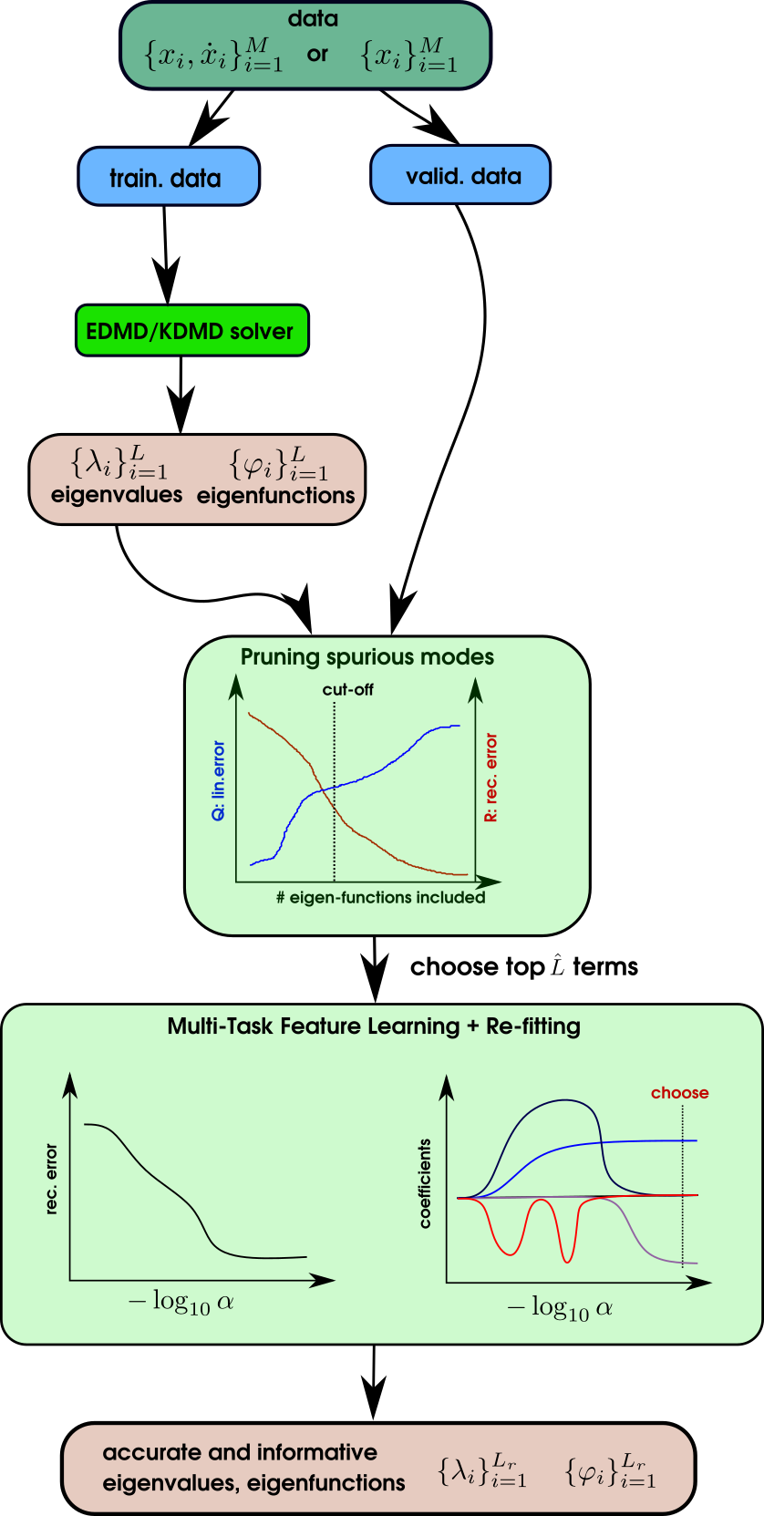
Figure 3: Schematic illustrating the idea of sparse identification of Koopman-invariant subspaces for EDMD and KDMD.

3.2.1 Relationship between sparsity-promoting DMD, Kou’s criterion and multi-task feature learning

For simplicity, neglecting the ElasticNet part (i.e., using $\rho=1$), eq. 36 with $L$ modes leads to a multi-task Lasso problem,

$$\min_{\mathbf{B}^{{}^{\prime}}\in\mathbb{C}^{L\times N}}\frac{1}{2M}\lVert\mathbf{X}-\mathbf{\hat{\Psi}}_{L,\textrm{scaled}}\mathbf{B}^{{}^{\prime}}\rVert_{F}^{2}+\alpha\lVert\mathbf{B}^{{}^{\prime}}\rVert_{2,1}.$$ (39)

Recall that in spDMD (Jovanović et al., 2014), DMD modes $\phi_{1},\ldots,\phi_{L}$ with $\lVert\phi_{i}\rVert_{2}=1$ remain the same as standard DMD. Similariy, if we posit a structural constraint on $\mathbf{B}^{{}^{\prime}}$ in eq. 39 by enforcing the modes as those from DMD, then there exist $\alpha_{1},\ldots,\alpha_{L}$ such that,

$$\mathbf{B}^{{}^{\prime}}=\begin{bmatrix}\alpha_{1}&&\\ &\ddots&\\ &&\alpha_{L}\end{bmatrix}\begin{bmatrix}\phi_{1}^{\textrm{T}}\\ \vdots\\ \phi_{L}^{\textrm{T}}\end{bmatrix}.$$ (40)

Note the fact that $\lVert\mathbf{B}^{{}^{\prime}}\rVert_{2,1}=\sum_{i}^{L}\lvert\alpha_{i}\rvert$. Hence, we recover the $\ell_{1}$ optimization step in the spDMD (Jovanović et al., 2014) from eq. 39 as,

$$\min_{\alpha_{1},\ldots,\alpha_{L}\in\mathbb{C}}\frac{1}{2M}\Bigg{\|}\mathbf{X}-\begin{bmatrix}1&\ldots&1\\ \vdots&\vdots&\vdots\\ e^{({M-1})\Delta t\lambda_{i_{1}}}&\ldots&e^{({M-1})\Delta t\lambda_{i_{L}}}\end{bmatrix}\begin{bmatrix}\alpha_{1}&&\\ &\ddots&\\ &&\alpha_{L}\end{bmatrix}\begin{bmatrix}\phi_{1}^{\textrm{T}}\\ \vdots\\ \phi_{L}^{\textrm{T}}\end{bmatrix}\Bigg{\|}^{2}_{F}+\alpha\sum_{i=1}^{L}\lvert\alpha_{i}\rvert,$$ (41)

where $\phi_{1},\ldots,\phi_{L}$ are the DMD modes corresponding to eigenvalues as $\lambda_{1},\ldots,\lambda_{L}$. Hence, multi-task feature learning solves a less constrained optimization than spDMD in the context of DMD.

Kou & Zhang (2017) proposed an empirical criterion for mode selection by ordering modes with “energy” $I_{i}$ defined as

$$I_{i}=\sum_{j=1}^{M}|\alpha_{i}e^{(j-1)\Delta t\lambda_{i}}|=\begin{cases}\frac{|\alpha_{i}|(1-\lvert e^{\Delta t\lambda_{i}}\rvert^{M})}{1-\lvert e^{\Delta t\lambda_{i}}\rvert},&\text{if }\lvert e^{\Delta t\lambda_{i}}\rvert\neq 1,\\ M|\alpha_{i}|,&\text{otherwise},\end{cases}.$$ (42)

From an optimization viewpoint, consider a posteriori prediction matrix $\mathbf{X}_{\textrm{DMD}}$ from DMD

$$\mathbf{X}\approx\mathbf{X}_{\textrm{DMD}}=\begin{bmatrix}1&\ldots&1\\ \vdots&\vdots&\vdots\\ e^{({M-1})\Delta t\lambda_{1}}&\ldots&e^{({M-1})\Delta t\lambda_{{L}}}\end{bmatrix}\begin{bmatrix}\alpha_{1}&&\\ &\ddots&\\ &&\alpha_{L}\end{bmatrix}\begin{bmatrix}\phi_{1}^{\textrm{T}}\\ \vdots\\ \phi_{L}^{\textrm{T}}\end{bmatrix},$$ (43)

where $\mathbf{X}_{\textrm{DMD}}$ is determined from DMD using the snapshot pair $(\mathbf{X},\mathbf{X}^{{}^{\prime}})$. $\mathbf{X}_{\textrm{DMD}}$ is a rank-1 summation of contributions from different modes (Schmid, 2010). Hence, a general mode selection technique with a user-defined preference weighting $\mathbf{w}$ is the following weighted $\ell_{0}$ nonconvex optimization problem:

$$\min_{\mathbf{a}\in\mathbb{C}^{L}}\Bigg{\lVert}\mathbf{X}_{\textrm{DMD}}-\begin{bmatrix}1&\ldots&1\\ \vdots&\vdots&\vdots\\ e^{({M-1})\Delta t\lambda_{1}}&\ldots&e^{({M-1})\Delta t\lambda_{{L}}}\end{bmatrix}\textrm{diag}(\mathbf{a})\begin{bmatrix}\phi_{1}^{\textrm{T}}\\ \vdots\\ \phi_{L}^{\textrm{T}}\end{bmatrix}\Bigg{\rVert}^{2}_{F}+\lambda\lVert\mathbf{a}\rVert_{\mathbf{w},0}$$ (44)

where $\lVert\mathbf{a}\rVert_{\mathbf{w},0}\triangleq\sum_{i}w_{i}|a_{i}|^{0}$, $|a_{i}|^{0}$ is one if $a_{i}\neq 0$ and zero otherwise. Note that this pseudo-norm can be viewed as a limiting case of a weighted composite sine function smoothed $\ell_{0}$ regularization (Wang et al., 2019).

To solve this non-convex optimization problem, compared to the popular $\ell_{1}$ relaxation method such as the one in sparsity-promoting DMD, a less-known but rather efficient way is iterative least-squares hard thresholding. This has been used in sparse identification of dynamical systems (SINDy) (Brunton et al., 2016b), and convergence to a local minimum has been proved (Zhang & Schaeffer, 2019). Indeed, a more rigorous framework that generalizes such an algorithm is the proximal gradient method (Parikh et al., 2014). Much like Newton’s method is a standard tool for unconstrained smooth optimization, the proximal gradient method is the standard tool for constrained non-smooth optimization. Here, it is straightforward to derive the iterative algorithm that extends to the weighted $\ell_{0}$ norm from step $k$ to step $k+1$ as

$$\mathbf{a}^{k+1}=\textrm{prox}_{\frac{\lambda}{2}\eta_{k}\lVert\cdot\rVert_{\mathbf{w},0}}(\mathbf{a}^{k}-\eta_{k}\nabla_{\mathbf{a}}\mathcal{Q}(\mathbf{a}^{k})),$$ (45)

where

$$\mathcal{Q}(\mathbf{a})=\frac{1}{2}\Bigg{\lVert}\mathbf{X}_{\textrm{DMD}}-\begin{bmatrix}1&\ldots&1\\ \vdots&\vdots&\vdots\\ e^{({M-1})\Delta t\lambda_{1}}&\ldots&e^{({M-1})\Delta t\lambda_{{L}}}\end{bmatrix}\textrm{diag}(\mathbf{a})\begin{bmatrix}\phi_{1}^{\textrm{T}}\\ \vdots\\ \phi_{L}^{\textrm{T}}\end{bmatrix}\Bigg{\rVert}^{2}_{F},$$ (46)

and $\eta_{k}$ is the step-size at step $k$. Notice that the weighted $\ell_{0}$ norm is a separable sum of $a_{i}$. After some algebra, we have the proximal operator as

$$\textrm{prox}_{\frac{\lambda}{2}\eta_{k}\lVert\cdot\rVert_{\mathbf{w},0}}(\mathbf{a})=\begin{bmatrix}\mathcal{H}_{\sqrt{\lambda\eta_{k}}}(a_{1}/\sqrt{w_{1}})&\ldots&\mathcal{H}_{\sqrt{\lambda\eta_{k}}}(a_{L}/\sqrt{w_{L}})\end{bmatrix}^{\textrm{T}},$$ (47)

where $\mathcal{H}_{\sqrt{\lambda\eta_{k}}}(a)$ is an element-wise hard thresholding operator defined as $a$ if $|a|<\sqrt{\lambda\eta_{k}}$ and zero otherwise.

Particularly, if one considers the initial step-size to be extremely small $\eta_{1}\ll 1$, then the second term in eq. 45 can be neglected. Thus, for $i=1,\ldots,L$, with the following weighting scheme that penalizes fast decaying modes:

$$w_{i}=1/\beta_{i}^{2},\quad\beta_{i}=\begin{cases}\frac{1-\lvert e^{\Delta t\lambda_{i}}\rvert^{M}}{1-\lvert e^{\Delta t\lambda_{i}}\rvert},&\text{if }\lvert e^{\Delta t\lambda_{i}}\rvert\neq 1,\\ M,&\text{otherwise},\end{cases}$$ (48)

one immediately realizes the thresholding criterion for $i$-th entry of $\mathbf{a}$ becomes

$$\sqrt{\lambda\eta_{k}}>|\alpha_{i}/\sqrt{w_{i}}|=|\alpha_{i}\beta_{i}|.$$ (49)

Then plugging eq. 48 in eq. 45, the first iteration in eq. 45 reduces to mode selection with Kou’s criterion in eq. 42. Normally, $\beta_{i}$ is very large for unstable modes and small for decaying modes. It is important to note that a) such a choice of $\mathbf{w}$ preferring unstable/long-lasting modes over decaying modes is still user-defined; 2) Optimization is in an a priori sense to obtain DMD. Thus, the insufficiency of the a priori formulation to account for temporal evolution is indeed compensated by this criterion, while DMD in an a posteriori formulation (e.g., sparsity-promoting DMD) includes such a effect implicitly in the optimization. Hence, it is possible that in some circumstances spDMD and Kou’s criterion could achieve similar performance (Kou & Zhang, 2017).

Lastly, as summarized in fig. 4, it is important to mention the similarities and differences between spKDMD and spDMD: 1) spKDMD will refit Koopman modes while spDMD does not; and 2) The amplitude for all the modes in spKDMD is fixed as unity while it has to be determined in spDMD.

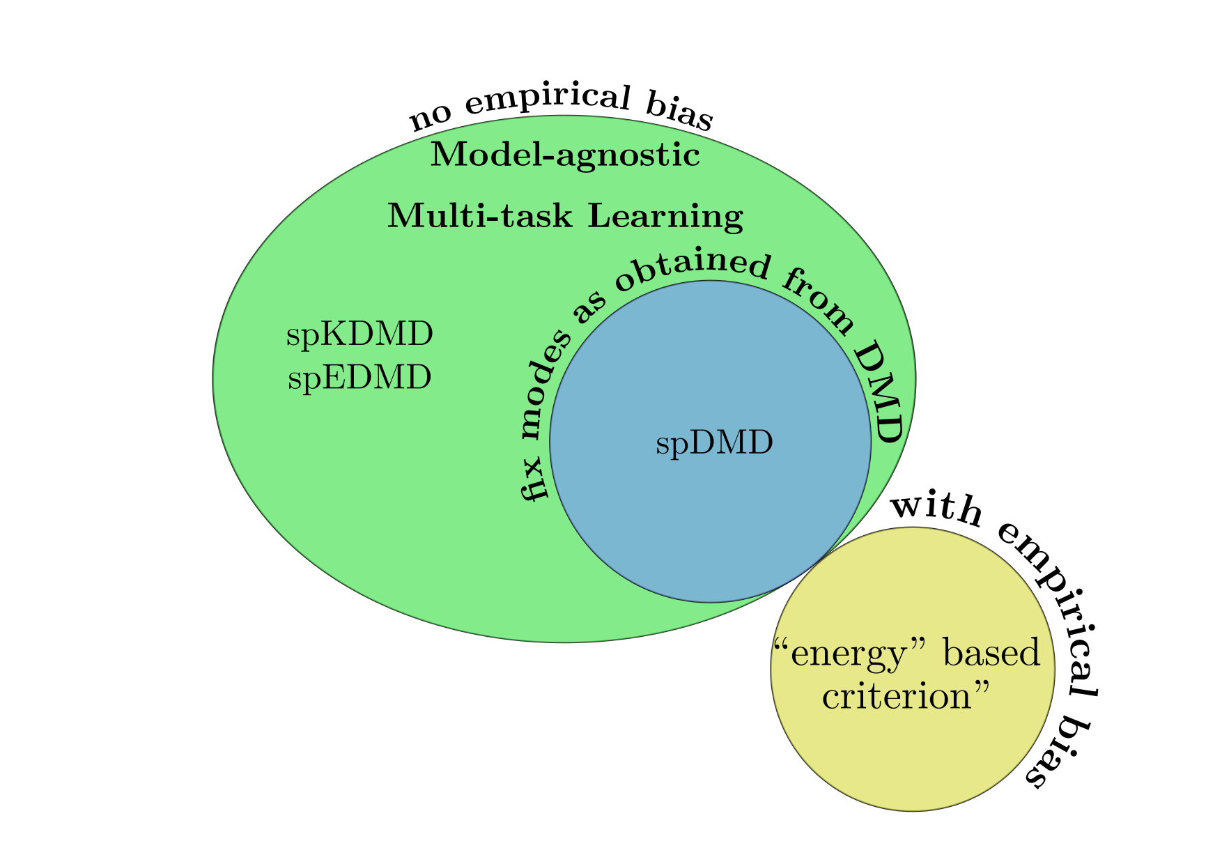
Figure 4: Differences and similarities among existing mode selection methods.

3.3 Hyper-parameter selection

For simplicity, hyper-parameter selection for KDMD is only discussed in this section. To fully determine a kernel in KDMD, one would have to choose the following:

1. kernel type,

2. kernel parameters, e.g., scale parameters $\sigma$,

3. rank truncation $r$.

In this work, for simplicity, we fix the kernel type to be an isotropic Gaussian. Motivated by previous work on error evaluation in Koopman modes by Zhang et al. (2017), we consider evaluation with cross validation on a priori mean normalized accuracy defined in eqs. 50 and 51 for $i$-th eigenfunction,

$$\textrm{discrete form: }{Q}_{i}^{a}=\frac{1}{M-1}\sum_{j=1}^{M-1}\frac{|\varphi_{i}(\mathbf{x}_{j+1})-\lambda_{i}\varphi_{i}(\mathbf{x}_{j})|}{\sqrt{\frac{1}{M}\sum_{k=1}^{M}\varphi_{i}^{*}(\mathbf{x}_{k})\varphi_{i}(\mathbf{x}_{k})}}$$ (50)

$$\textrm{continuous form: }{Q}_{i}^{a}=\frac{1}{M}\sum_{j=1}^{M}\frac{|\dot{\mathbf{x}}_{j}\cdot\nabla_{\mathbf{x}}\varphi_{i}(\mathbf{x}_{j})-\lambda_{i}\varphi_{i}(\mathbf{x}_{j})|}{\sqrt{\frac{1}{M}\sum_{k=1}^{M}\varphi_{i}^{*}(\mathbf{x}_{k})\varphi_{i}(\mathbf{x}_{k})}}$$ (51)

on validation data for different number of rank truncation and kernel parameters.

Note that evaluation on maximal instead of mean normalized accuracy would lead to the error metric to be strongly dependent on the local sparsity of training data in the feature space. This is particularly true for a single trajectory for a high-dimensional dynamical system is used, and random shuffled cross validation is performed (Pan & Duraisamy, 2018).

For each set of hyperparameters, we first compute the number of eigenfunctions of which the error defined in eqs. 50 and 51 is below a certain threshold on both training and validation data for each fold of cross validation. Then we compute the average number of such eigenfunctions over all folds which indicates the quality of the corresponding subspace. Finally, we plot the average number versus rank truncation $r$ and kernel scale parameters $\sigma$ to select hyperparameters.

3.4 Implementation

We implement the described framework in Python with moderate parallelism in each module. We use scipy.special.hermitenorm (Jones et al., 2001–) to generate normalized Hermite polynomials and MultiTaskElasticNet in the scikit-learn (Pedregosa et al., 2011) for multi-task feature learning where we set the maximal iteration as $10^{5}$ and tolerance as $10^{-12}$. MPI parallelism using mpi4py (Dalcin et al., 2011) is used for the grid search in hyperparameter selection. To prepare data with hundreds of gigabytes collected from high fidelity simulations, a distributed SVD written in C++ named Parallel Data Processing (PDP) Tool is developed for dimension reduction. A brief description of this tool is given in appendix D.

4 Results and Discussion

4.1 2D fixed point attractor with the known finite Koopman-invariant subspace

We first consider a simple fixed point nonlinear dynamical system which has an analytically determined, finite-dimensional non-trivial Koopman-invariant subspace (Brunton et al., 2016a; Kaiser et al., 2017) to show the effectiveness of proposed method. We consider a continuous-time formulation. The governing equation for the dynamical system is given as follows,

$$\dot{x}_{1} =\mu x_{1},$$ (52)

$$\dot{x}_{2} =\lambda(x_{2}-x_{1}^{2}),$$ (53)

where $\mu=-0.05,\lambda=-1$. One natural choice of the minimal Koopman eigenfunctions that linearly reconstructs the state is (Brunton et al., 2016a)

$$\varphi_{1}(\mathbf{x})=x_{2}-\lambda x_{1}^{2}/(\lambda-2\mu),\quad\varphi_{2}(\mathbf{x})=x_{1},\quad\varphi_{3}(\mathbf{x})=x_{1}^{2}$$ (54)

with eigenvalues $\lambda=-1$, $\mu=-0.05$, $2\mu=-0.1$ respectively.

The way we generate training, validation, and testing data is described below with distribution of the data shown in fig. 5,

1. training data: a point cloud with $M=1600$ pairs of $\{\mathbf{x}^{(i)},\mathbf{\dot{x}}^{(i)}\}_{i=1}^{M}$, is generated by Latin hypercube sampling (Baudin et al., 2015) within the domain $x_{1},x_{2}\in[-0.5,0.5]$.

2. validation data: a single trajectory with initial condition as $x_{1}(0)=x_{2}(0)=0.4$, sampling time interval $\Delta t=0.03754$ from $t=0$ to $t=30$.

3. testing data: a single trajectory with initial condition as $x_{1}(0)=x_{2}(0)=-0.3$, sampling time interval $\Delta t=0.06677$ from $t=0$ to $t=40$.

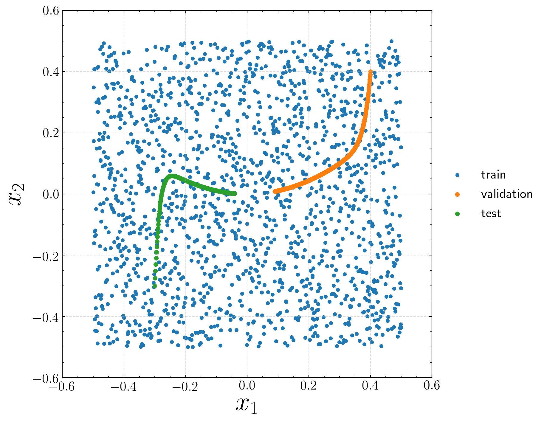
Figure 5: Data distribution for 2D fixed point attractor.

As an illustration, we consider two models to approximate the Koopman operator from training data:

1. a continuous-time EDMD with normalized Hermite polynomials up to fifth order with $L=36$ features,

2. a continuous-time KDMD with isotropic Gaussian kernel $\sigma=2$ with reduced rank $r=L=36$.

Details of the above choices based on the steps of hyperparameter selection in section 3.3 are given in section C.1.

4.1.1 Results for continuous-time EDMD with mode selection

As displayed in fig. 6, we begin with an error analysis of all of the eigenmodes on validation data in fig. 5 according to linearly evolving error $Q$ defined in eq. 29 and $R$ defined in eq. 31. From the left subfigure in fig. 6, considering both the linearly evolving error and the quality of the reconstruction, we choose the cut-off threshold at $\hat{L}=10$. We observe a sharp cut-off in the left subfigure in fig. 6 around the number of selected eigenmodes $\hat{L}=8$. This is a reasonable choice, since from the eigenvalues in the right subfigure in fig. 6, we notice the analytic Koopman eigenmodes are not covered until first 8 accurate eigenmodes are selected. Note that the legend in the right subfigure is ordered by the maximal deviation from linear evolution, e.g., the second most accurate mode is 34-th mode with zero eigenvalue. Indeed, the first four eigenfunctions (index=$1,34,35,36$) are redundant in terms of reconstruction in this problem . The fifth (index=$29$) and sixth (index=$33$) eigenmodes correspond to two of the analytic eigenfunctions that span the system, and the seventh (index=$32$) eigenmode is indeed the product of the fifth and sixth eigenfunctions. Similarly, the ninth and tenth eigenfunctions (index=$31,28$) also appear to be the polynomial combination of the true eigenfunctions.

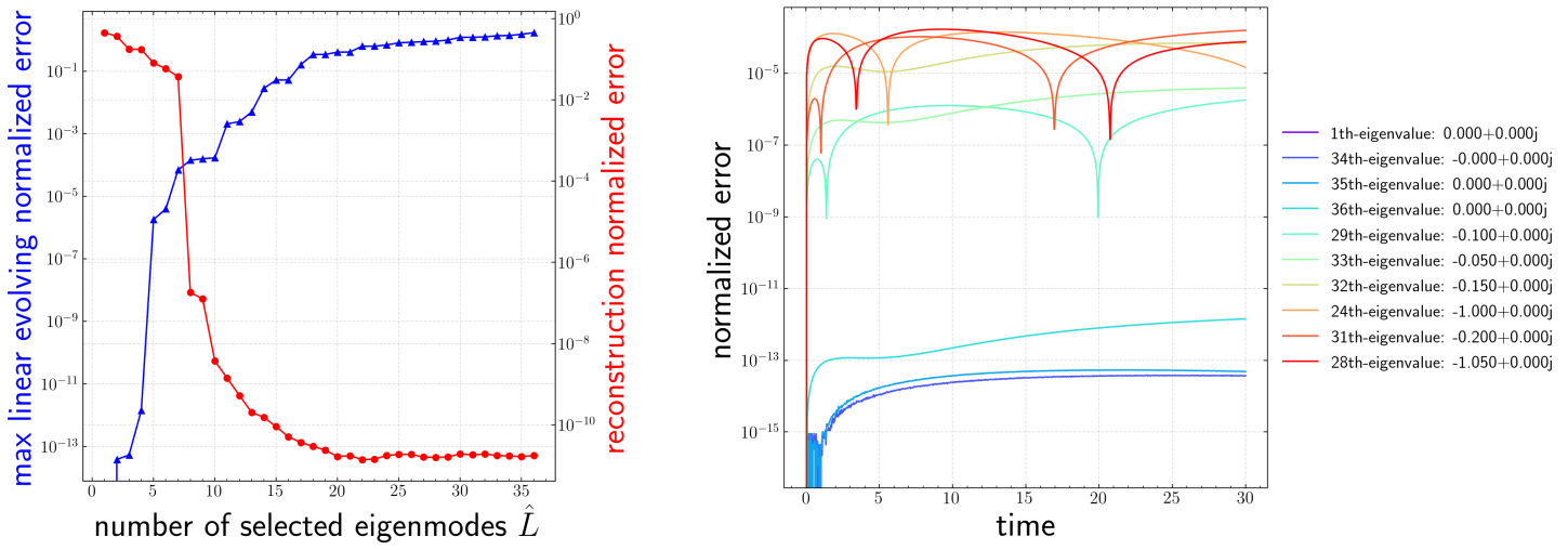
Figure 6: Error analysis of 36 eigenmodes from continuous-time EDMD for the 2D fixed point attractor. Left: trends of linearly evolving error $Q$ and reconstruction error $R$. Right: temporal evolution of relative error for top $\hat{L}=10$ accurate eigenmodes.

According to eq. 36, to further remove redundant modes, we perform multi-task feature learning on the $\hat{L}=10$ eigenmodes . The corresponding ElasticNet path is shown in fig. 7. Note that each $\alpha$ corresponds to a minimizer of eq. 36. To choose a proper $\alpha$ so as to find a proper Koopman-invariant subspace, it is advisable to check the trend of the normalized reconstruction error and number of non-zero features. Given the dictionary, for simple problems for which there exists an exact Koopman-invariant subspace that also spans system state, a proper model can be obtained by selecting $\alpha\approx 10^{-6}$ which ends up with only 3 eigenfunctions as shown in fig. 7. Moreover, as is common for EDMD with polynomial basis (Williams et al., 2014, 2015), a pyramid of eigenvalues appears in fig. 7.

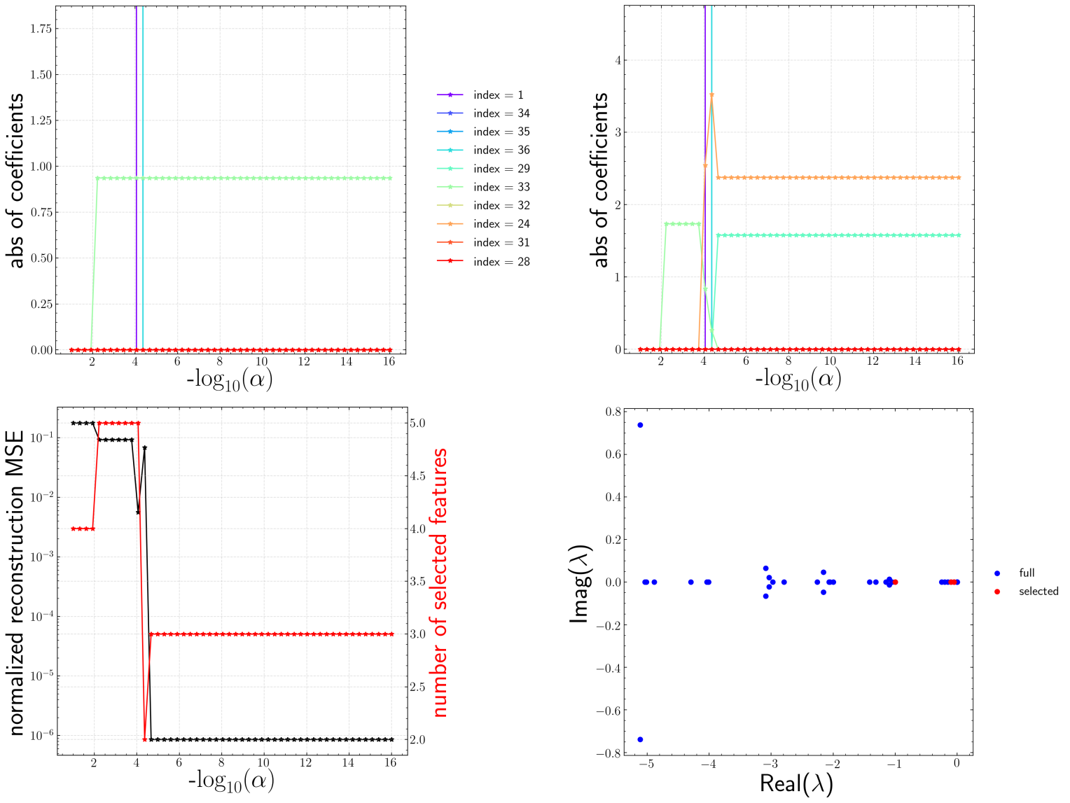
Figure 7: Result of multi-task feature learning on top $\hat{L}=10$ accurate eigenmodes from continuous-time EDMD for the 2D fixed point attractor. Top left: ElasticNet path for $x_{1}$. Top right: ElasticNet path for $x_{2}$. Bottom left: trends of normalized reconstruction error and number of non-zero terms versus $\alpha$. Bottom right: selected continuous-time eigenvalues.

As shown in fig. 8, both the identified eigenvalues, and contour of the phase angle and magnitude of selected eigenfunctions from spEDMD match the analytic eigenfunctions given in eq. 54 very well. As expected, the prediction on unseen testing data is also excellent. Note that the indices of true eigenfunctions $\varphi_{1}$, $\varphi_{2}$ and $\varphi_{3}$ ordered by Kou’s criterion in eq. 42 are 8, 5 and 6. In this case, all of the true eigenfunctions are missing in the top 3 modes chosen by Kou’s criterion. Indeed, the top 3 modes chosen by Kou’s criterion have nearly zero eigenvalues.

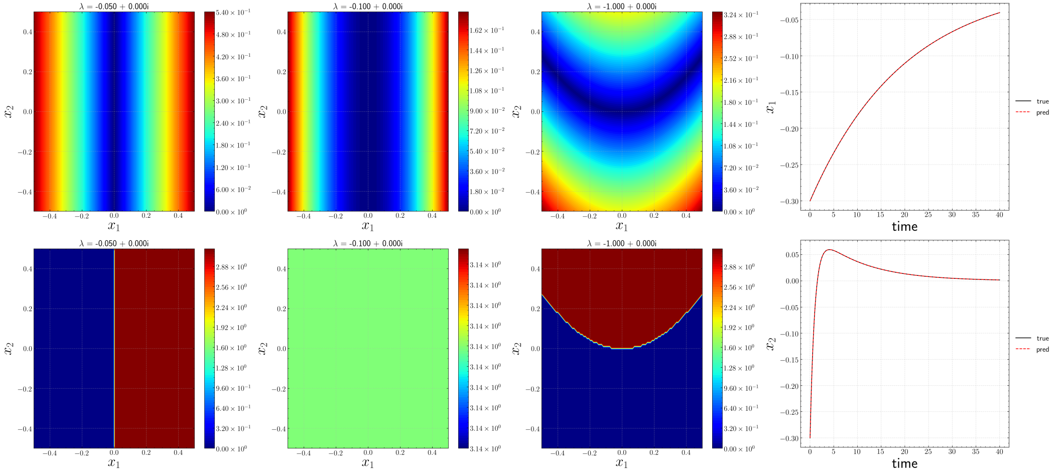
Figure 8: Sparsely selected eigenfunctions and eigenvalues from continuous-time EDMD for 2D fixed point attractor with corresponding prediction on testing data with an unseen initial condition $x_{1}(0)=x_{2}(0)=-0.3$. From left to right, the top three figures show contours of magnitude of eigenfunctions, while the bottom three figures are those of phase angle of eigenfunctions. Last column: comparison between prediction and ground truth for an unseen testing trajectory.

4.1.2 Results of continuous-time KDMD with mode selection

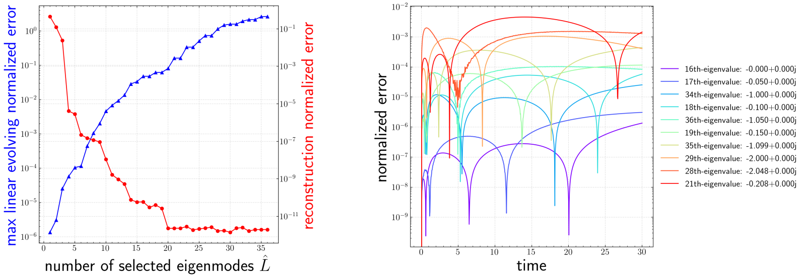
Figure 9: Error analysis of 36 eigenmodes from continuous-time KDMD for the 2D fixed point attractor. Left: trends of linearly evolving error $Q$ and reconstruction error $R$. Right: temporal evolution of relative error for top $\hat{L}=10$ accurate eigenmodes.

The mode selection algorithm presented above can be applied in precisely the same form to KDMD, given a set of eigenfunctions and eigenvalues. Error analysis of eigenfunctions is shown in fig. 9, from which we choose $\hat{L}=10$ as well. As before, eigenvalues ordered by maximal deviation from linear evolution are shown in the legend in the right subfigure in fig. 9. Again, in the left subfigure in fig. 9, we observe a sharp decrease in the reconstruction error after the 4 most accurate modes are included. This is expected, as the second to fourth most accurate modes are analytically exact from the right subfigure. As shown in figs. 10 and 11, it is confirmed that that both spEDMD and spKDMD arrive at the same analytic eigenfunctions with difference up to a constant factor. It should be noted that, although polynomials are not analytically in the RKHS (Minh, 2010), good approximations can still be achieved conditioned on the data we have, i.e., $x_{1},x_{2}\in[-0.5,0.5]$. Again, the indices of true eigenfunctions $\varphi_{1}$ to $\varphi_{3}$ ordered by Kou’s criterion are 8, 2 and 3. Hence, $\varphi_{1}$ is missing in the top 3 modes chosen by Kou’s criterion. Similarly, the first mode chosen by Kou’s criterion has a zero eigenvalue.

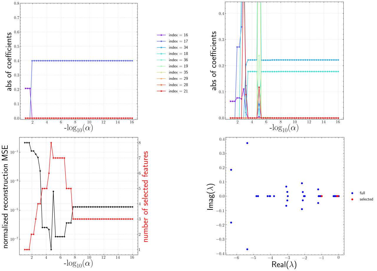
Figure 10: Result of multi-task feature learning on top $\hat{L}=10$ accurate eigenmodes from continuous-time KDMD for the 2D fixed point attractor. Top left: ElasticNet path for $x_{1}$. Top right: ElasticNet path for $x_{2}$. Bottom left: trends of normalized reconstruction error and number of non-zero terms versus $\alpha$. Bottom right: selected continuous-time eigenvalues.

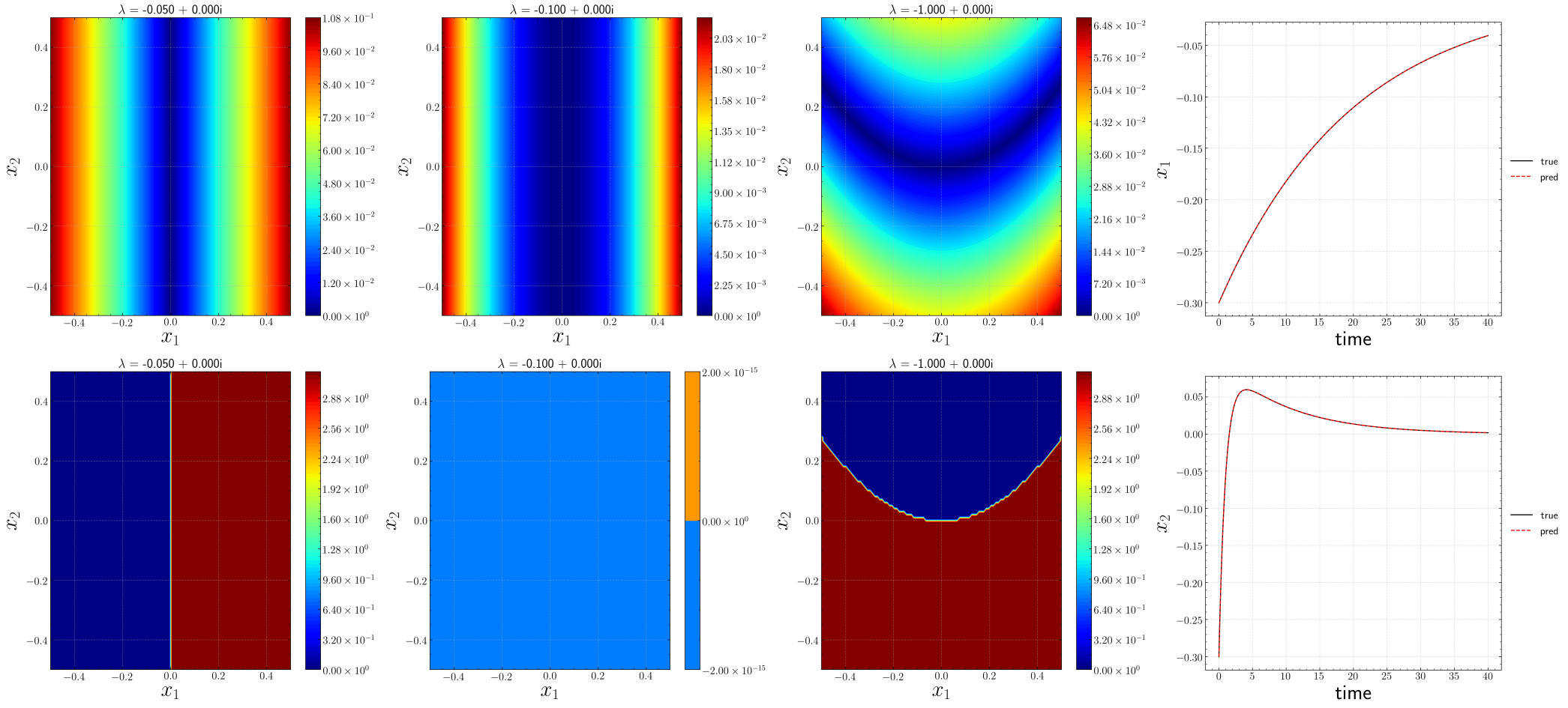
Figure 11: Sparsely selected eignefunctions and eigenvalues from continuous-time KDMD for 2D fixed point attractor with corresponding prediction on testing data with an unseen initial condition $x_{1}(0)=x_{2}(0)=-0.3$. From left to right, the top three figures show contours of the magnitude of eigenfunctions, while the bottom three figures are those of phase angle of eigenfunctions. Last column: comparison between predictions and ground truth for an unseen testing trajectory.

4.1.3 Effect of SVD regularization

SVD truncation is a standard regularization technique in the solution of a potentially ill-conditioned linear system. In the standard EDMD in eq. 7 - for example - $\mathbf{G}$ could be potentially ill-conditioned, leading to spurious eigenvalues in $\mathbf{K}$. Hence, Williams et al. (2014) recommend SVD truncation in eq. 8 to obtain a robust solution of $\mathbf{K}$. Effectively, it shrinks the number of EDMD/KDMD modes. It has to be recognized, however, that the mode reduction from SVD truncation is not the same as mode selection. Most importantly, one should not confuse numerical spuriousness from poor numerical conditioning with functional spuriousness from the orthogonal projection error of the Koopman operator (Korda & Mezić, 2018b). Indeed, SVD truncation does not always lead to better approximation of a Koopman-invariant subspace. It is rather a linear dimension reduction that optimally preserves the variance in the feature space conditioned on the training data without knowing the linear evolution property of each feature.

For demonstration, we take the above fixed point attractor system where we use the same data and standard EDMD algorithm with the same order of Hermite polynomials. The results of prediction on the unseen testing data shown in fig. 12 indicate that even though only 3 eigenfunctions (indeed 3 features in the Hermite polynomial) are required, standard EDMD fails to identify the correct eigenfunctions with 26 SVD modes while the results improve with 31 modes retained. The sensitivity of standard EDMD with respect to SVD truncation is likely a result of the use of normalized Hermite polynomials where SVD truncation would lead to a strong preference over the subspace spanned by the higher order polynomials. We did not observe such a sensitivity for KDMD, unless the subspace is truncated below 10 modes.

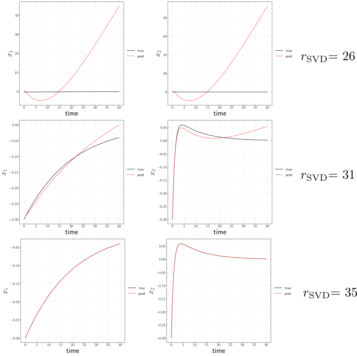
Figure 12: Standard EDMD prediction on unseen trajectory with different SVD truncations for fixed point attractor.

4.2 Two-dimensional, transient flow past a cylinder

As a classical example for Koopman analysis in fluid dynamics (Bagheri, 2013; Williams et al., 2014; Otto & Rowley, 2019), transient two-dimensional flow past cylinder (fig. 13) is considered at different Reynolds numbers ($\Rey={U_{\infty}D}/{\nu}$), where $U_{\infty}=1$ is the freestream velocity, $D=2$ is the diameter of the cylinder, and $\nu$ is the kinematic viscosity. The two-dimensional incompressible Navier–Stokes equations govern the dynamics with far-field boundary conditions for pressure and velocity and no-slip velocity on the cylinder surface. Numerical simulations are performed using the icoFoam solver in OpenFOAM (Jasak et al., 2007) solving the 2D incompressible Navier-Stokes equations. We explore $Re=70,100,130$ by changing the viscosity. The pressure field is initialized with i.i.d Gaussian noise $\mathcal{N}(0,0.3^{2})$. The velocity is initialized with a uniform freestream velocity superimposed with i.i.d Gaussian noise $\mathcal{N}(0,0.3^{2})$. It should be noted that the noise is generated on the coarsest mesh shown in fig. 13, and interpolated to the finer meshes. Grid convergence with increasing mesh resolution is assessed by comparing the temporal evolution of the drag coefficient $C_{D}$ and lift coefficient $C_{L}$.

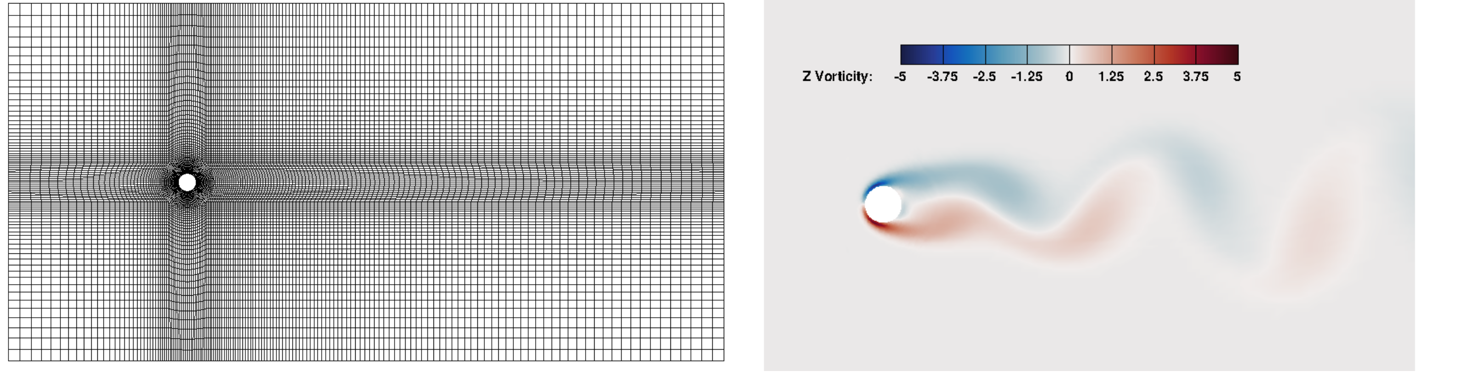
Figure 13: Left: illustration of computational mesh for 2D cylinder wake problem (coarsest). Right: contour of vorticity $\omega_{z}$ for $\Rey=70$ when vortex shedding is fully developed (t = 175).

Note that the dynamics of a cylinder wake involves four regimes: near-equilibrium linear dynamics, nonlinear algebraic interaction between equilibrium and the limit cycle, exponential relaxation rate to the limit cycle, and periodic limit cycle dynamics (Chen et al., 2012; Bagheri, 2013). Instead of considering data only from each of these regimes separately (Chen et al., 2012; Taira et al., 2019) or with only the last two regimes where exponential linear dynamics is expected (Bagheri, 2013), we start collecting data immediately after the flow field becomes unstable, and stop after the flow field experiences several limit cycles. Note that the regime with algebraic interaction is non-modal (Schmid, 2007), and therefore cannot be expressed as individual exponential terms (Bagheri, 2013). This becomes a challenging problem for DMD (Chen et al., 2012). The sampling time interval is $\Delta t=0.1t_{ref}$ where $t_{ref}=D/U_{\infty}$.

For each $\Rey$, 891 snapshots of full velocity field $U$ and $V$ with sampling time interval $\Delta t$ are collected as two matrices of size $N_{\textrm{grid}}\times N_{\textrm{snapshots}}$. Following this, each velocity component is shifted and scaled (normalized) between $[-1,1]$. Since space-filling sampling in any high-dimensional space would be extremely difficult, we split the trajectory into training, validation, and testing data by sampling with strides similar to the “even-odd” sampling scheme previously proposed by Otto & Rowley (2019). As illustrated in fig. 14, given index $i$, if $i\mod 3=0$, the $i$-th point belongs to training set while $i\mod 3=1$ corresponds to validation, and $i\mod 3=2$ for testing data. Consequently, the time interval in the training, testing, validation trajectory is tripled as $3\Delta t=0.3t_{ref}$.

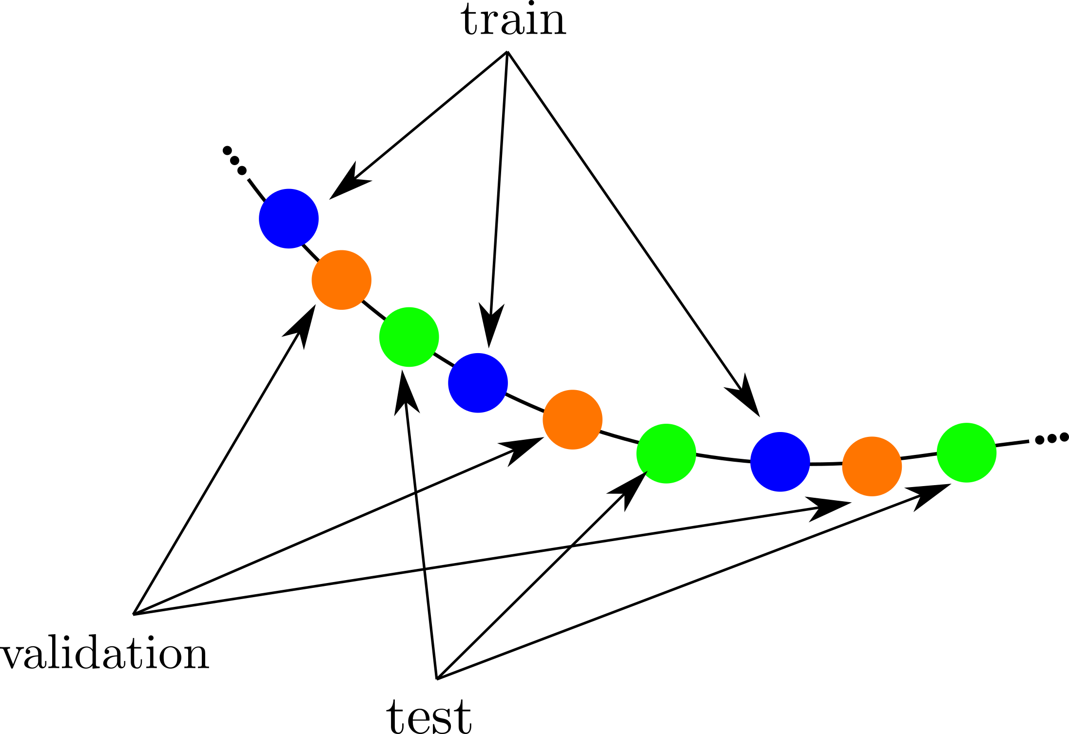
Figure 14: Illustration of splitting a uniformly sampled single trajectory in high dimensional phase space into training, validation and testing sets.

Thus, training, validation, and testing data are split into 297 snapshots each. Finally, we stack data matrices along the first axis corresponding to the number of grid points, and perform a distributed SVD described in section 3.4. For all three cases, the top 20 POD modes are retained, corresponding to 99% of kinetic energy. Next, we apply our algorithm to discrete-time KDMD with isotropic Gaussian kernel on this reduced-order nonlinear system. We choose the hyperparameters $\sigma=3$ and $r=180$. Further details are given in section C.2.

4.2.1 Results of discrete-time KDMD with mode selection

For all three Reynolds numbers, a posteriori error analysis is shown in fig. 15. A good choice of the number of accurate modes $\hat{L}$ retained for reconstruction is around 60 since the corresponding maximal deviation from linear evolution is still around 5% while the reconstruction error reaches a plateau after $\hat{L}>60$.

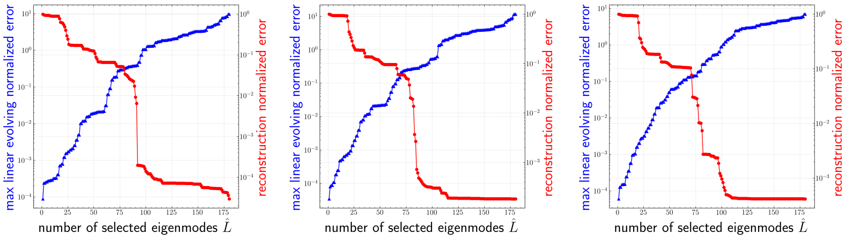
Figure 15: Trend of linear evolution error $Q$ and reconstruction error $R$ from discrete-time KDMD for the 20D cylinder wake flow case. Left: $\Rey=70$. Center: $\Rey=100$. Right: $\Rey=130$.

After the mode selection on validation data, a $\alpha$-family of solutions is obtained with corresponding reconstruction error and the number of non-zeros terms as shown in fig. 16. Note that the chosen solution is highlighted as blue circles. As shown in table 2, nearly half of the accurate KDMD eigenmodes identified are removed with the proposed sparse feature selection. Note that for all three cases, the number of selected modes (around 32 to 34) is still larger than that required in neural network models (around 10) (Pan & Duraisamy, 2020; Otto & Rowley, 2019). This is because the subspace spanned by KDMD/EDMD relies on a pre-determined dictionary rather than being data-adaptive like neural network models. Nevertheless, due to the additional expressiveness from non-linearity, we will see in section 4.2.3 that spKDMD performs significantly better than DMD (Schmid, 2010) and spDMD (Jovanović et al., 2014), while enjoying the property of convex optimization at a much lower computational cost than the inherently non-convex and computationally intensive neural network counterparts.

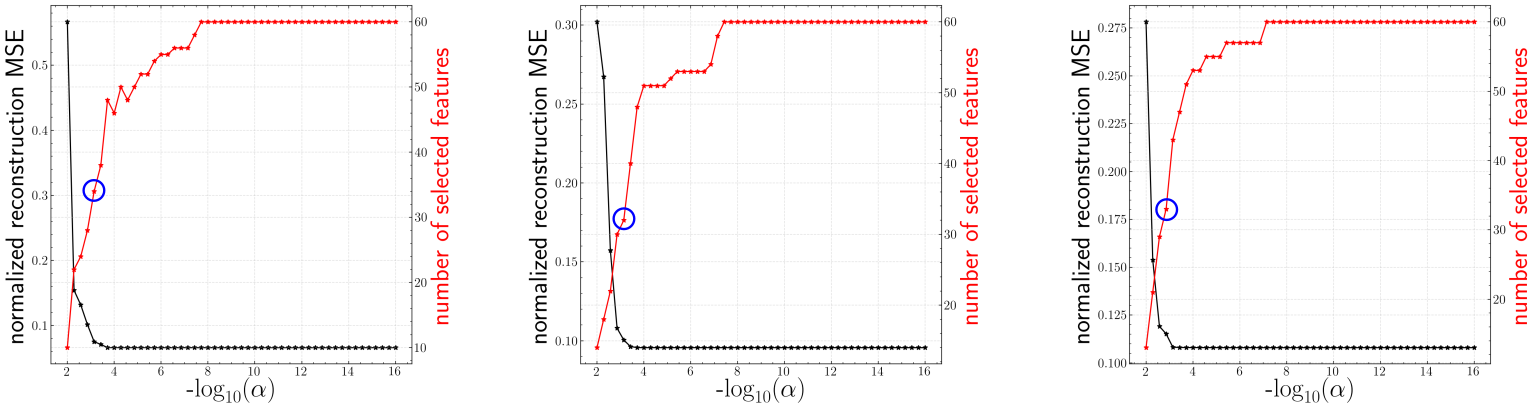
Figure 16: Variation of reconstruction error $R$ and number of non-zero terms for the 20D cylinder wake flow. Left: $\Rey=70$. Center: $\Rey=100$. Right: $\Rey=130$. Blue circle corresponds to selected $\alpha$.

	$Re=70$	$Re=100$	$Re=130$
$\alpha_{\textrm{select}}$	$7.19\times 10^{-4}$	$7.19\times 10^{-4}$	$1.39\times 10^{-3}$
number of selected modes	34	32	33
number of total modes	297	297	297
normalized reconstruction error $R$	0.075	0.105	0.113

Table 2: Summary of mode selection for discrete-time KDMD on 20D cylinder wake flow.

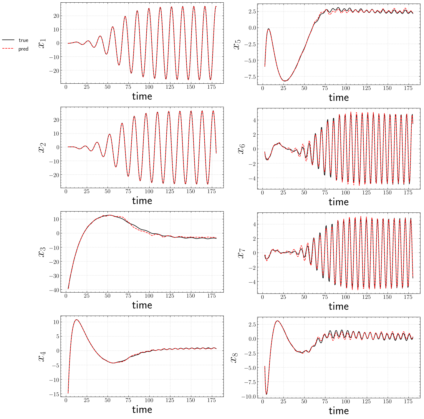
Figure 17: A posteriori prediction of testing trajectory for $\Rey=70$ in terms of top 8 POD coefficients with sparsity-promoting KDMD.

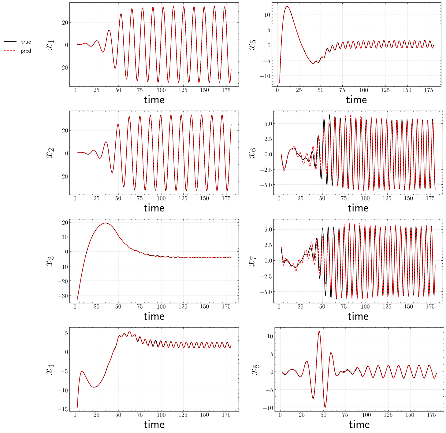
Figure 18: A posteriori prediction of testing trajectory for $\Rey=100$ in terms of top 8 POD coefficients with sparsity-promoting KDMD.

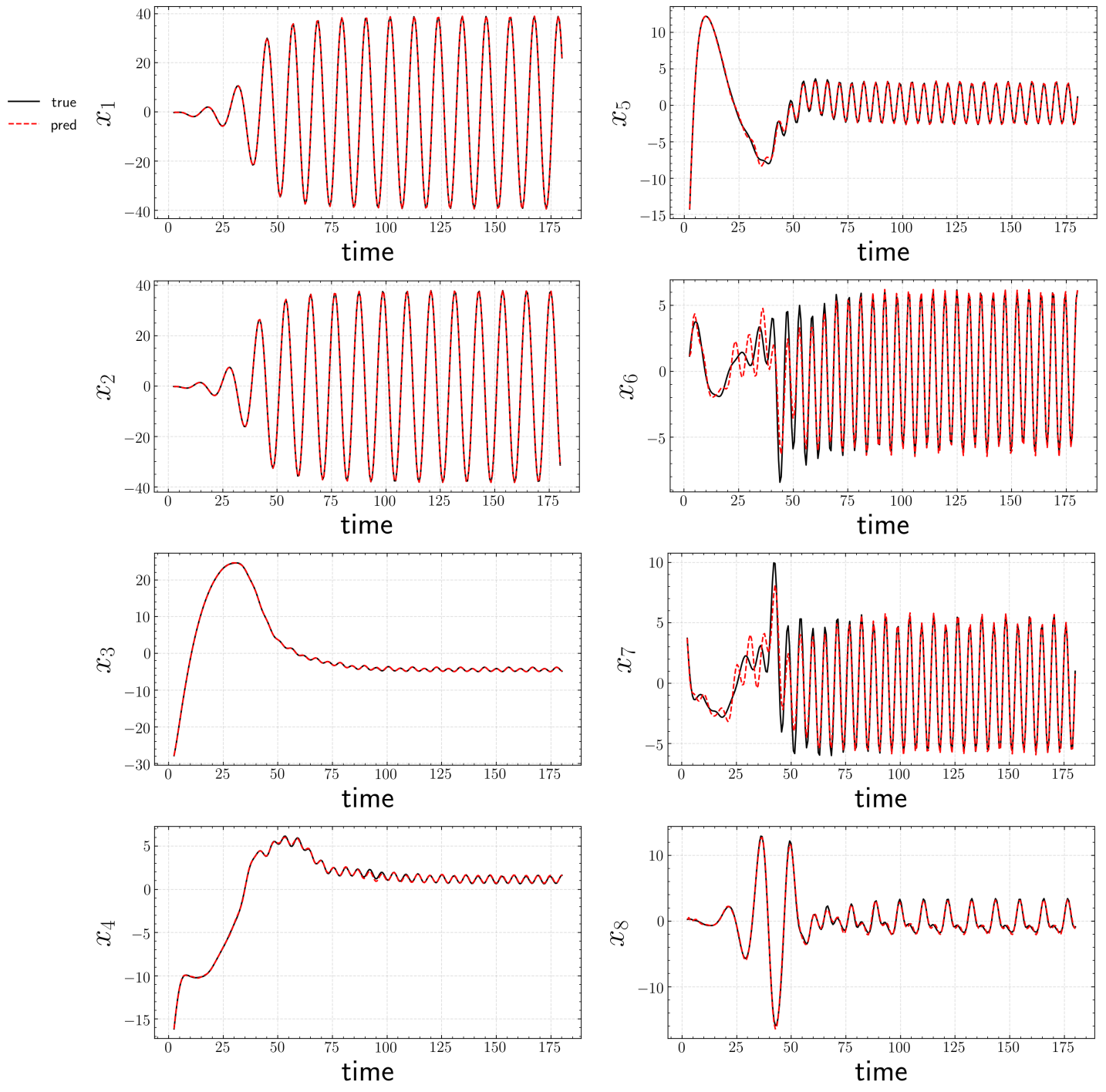
Figure 19: A posteriori prediction of testing trajectory for $\Rey=130$ in terms of top 8 POD coefficients with sparsity-promoting KDMD.

The predictions of the top 8 POD coefficients (denoted as $x_{1}$ to $x_{8}$) on testing data are displayed in figs. 17, 18 and 19. The results match very well with ground truth for all three cases. Figure 21 shows that there appear to be five clusters of selected eigenvalues while most of the modes are removed by the proposed algorithm. Similar observations were also made in (Bagheri, 2013) when DMD is applied to the full transient dynamics. This pattern consisting of a stable eigenvalue on the unit circle surrounded by several decaying eigenvalues is observed for all clusters. The stable eigenvalue contributes to limit-cycle behavior, while the decaying eigenvalues account for the transient phenomenon. Due to symmetry, only eigenvalues in the first quadrant are shown in the bottom row of fig. 21. It is observed that the frequency associated with the type-II cluster is approximately twice that of type-I. This is in good agreement with previous analytical results from the weakly non-linear theory (Bagheri, 2013). The frequency $f$ is normalized as $\textrm{St}=fD/U_{\infty}$, where St is the Strouhal number.

Recall that in the laminar parallel shedding region ($47<\Rey<180$), the characteristic Strouhal number $St$ scales with $-1/\sqrt{\Rey}$ (Fey et al., 1998). Therefore, it is expected that $St$ of both types tend toward higher frequency as $Re$ increases from 70 to 130. Further, it is interesting to note that the corresponding Strouhal numbers for lift and drag when the system is on the limit-cycle - $St_{L}$ and $St_{D}$ - coincide with the stable frequency of type-I and II respectively as indicated in fig. 21. This is due to the anti-symmetrical/symmetrical structure of the velocity field of type-I/II Koopman mode respectively as can be inferred from fig. 22. A schematic is is also shown in fig. 20.

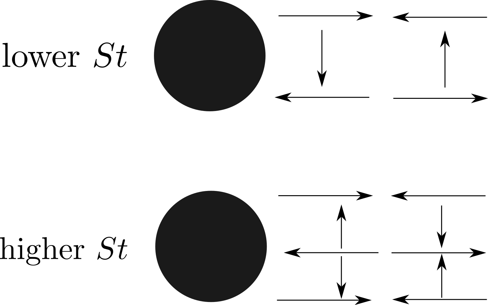
Figure 20: Illustration of the structure of velocity field for the lower (top) and higher frequency (bottom) Koopman modes. The arrow roughly indicates the velocity direction.

The higher frequency mode is symmetrical (along the freestream direction) in $U$ and anti-symmetrical in $V$. As a consequence, this only contributes to the oscillation of drag. The lower frequency mode is anti-symmetrical in $U$ and symmetrical in $V$, and only contributes to the oscillation of lift. Thus, the fluctuation in the lift mostly results from the stable mode in type-I, while that for drag results from the stable mode in type-II with twice the frequency.

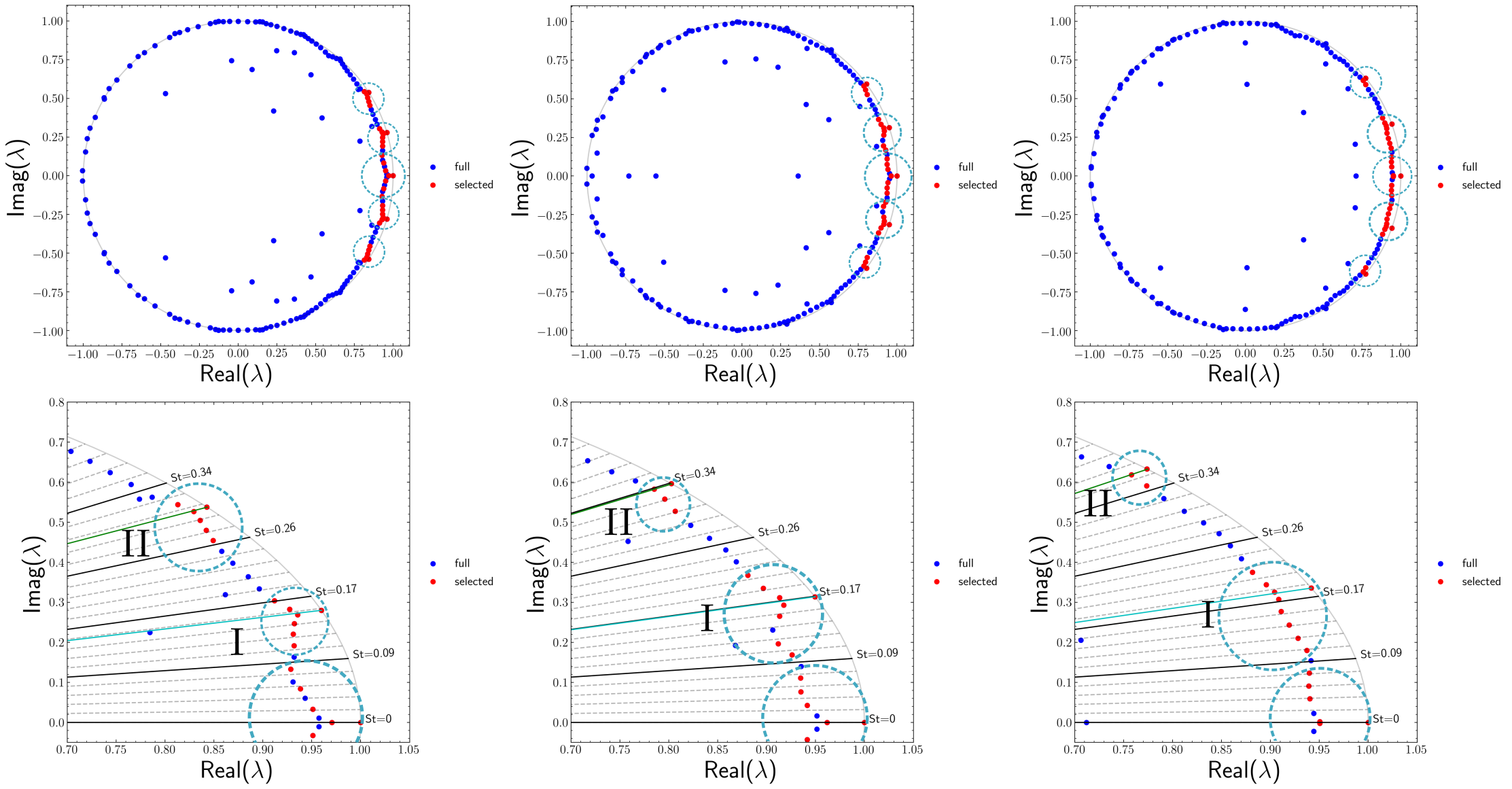
Figure 21: Discrete-time eigenvalue distribution of full KDMD and spKDMD. Left: $\Rey=70$. Center: $\Rey=100$. Right: $\Rey=130$. Blue dot: full KDMD eigenvalues. Red dot: spKDMD eigenvalues. Bottom row: zoomed. I and II correspond to two types of eigenvalue clusters of distinct frequencies, with each of them enclosed by cyan dashed circles. Green/cyan solid line correspond to $St_{D}$/$St_{L}$.

Finally, several representative Koopman modes from spKDMD for three $\Rey$ are shown in figs. 22, 23 and 24. For a better comparison of mode shapes, contributions from the stable modes of type-I and II with a threshold of 0.001 at $t=0$ is displayed in the top left of fig. 25. To remove the effect of time, the “envelope” of the mode shape, i.e., time average of the iso-contours is shown in the top right of fig. 25. From these results, we observe the following interesting phenomena:

• the minimal dimension of the Koopman-invariant subspace that approximately captures the limit cycle attractor for all three $\Rey$ that fall into laminar vortex shedding regime (White & Corfield, 2006) is five, which is consistent with previous multi-scale expansion analysis near the critical $\Rey$ (Bagheri, 2013).

• the lobes of stable Koopman modes in the type-I cluster show an approximately 50% larger width than those in a type-II cluster.

• similarity/colinearity among Koopman modes within each cluster is observed. Such a finding is previously reported in the theoretical analysis by Bagheri (2013). A similarity in spatial structure exists among the Koopman modes belonging to the same family, even though the structures are clearly phase lagged.

• as $\Rey$ increases from 70 to 130, mode shapes flatten downstream while expand upstream.

• at $\Rey=70$, the shear layer in the stable Koopman modes continues to grow within the computational domain. However, at $\Rey=100,130$, the shear layer stops growing after a certain distance that is negatively correlated with $\Rey$.

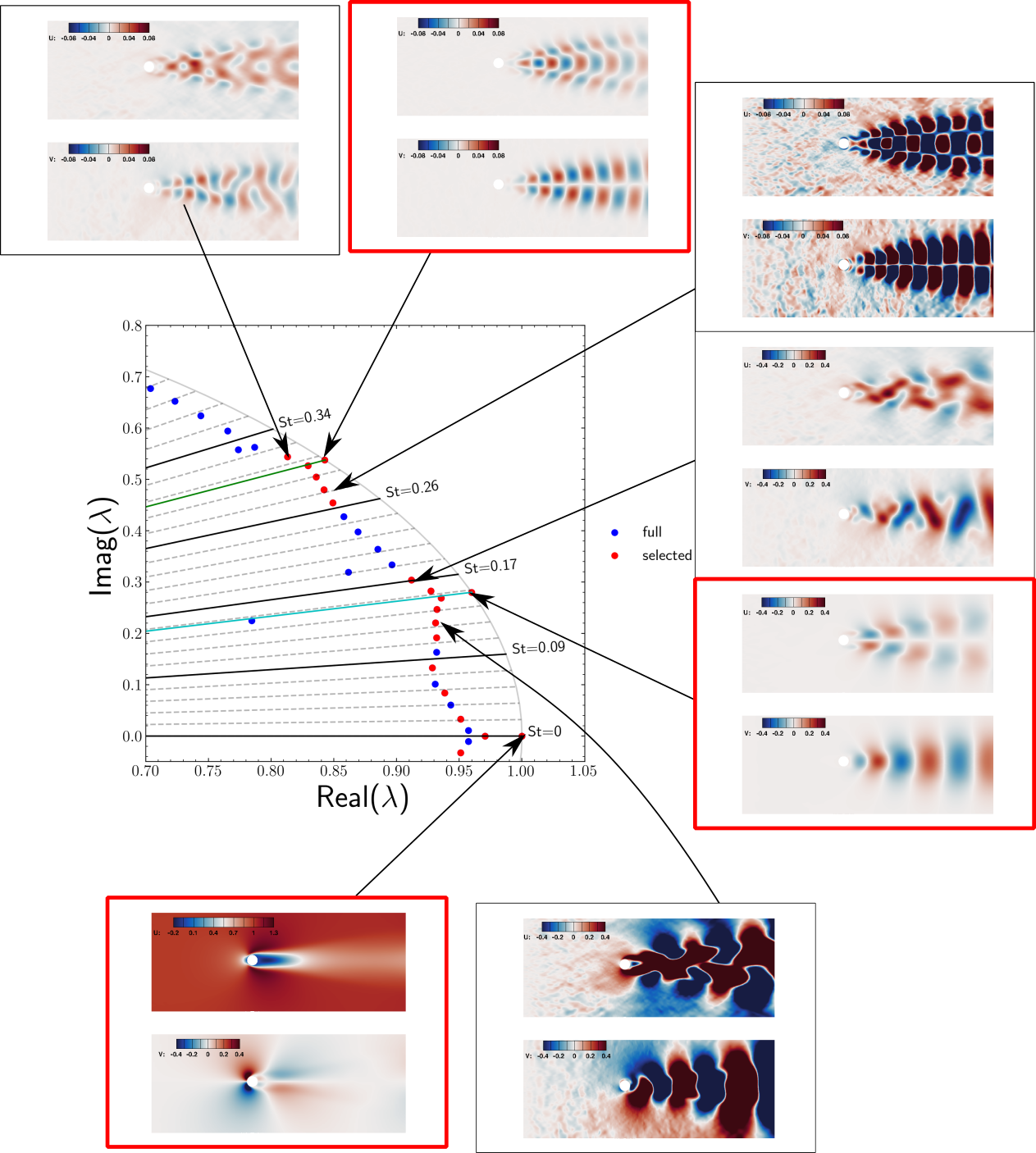
Figure 22: Contours of Koopman modes of $\Rey=70$ cylinder wake flow at $t=0$. Red squares indicate stable modes.

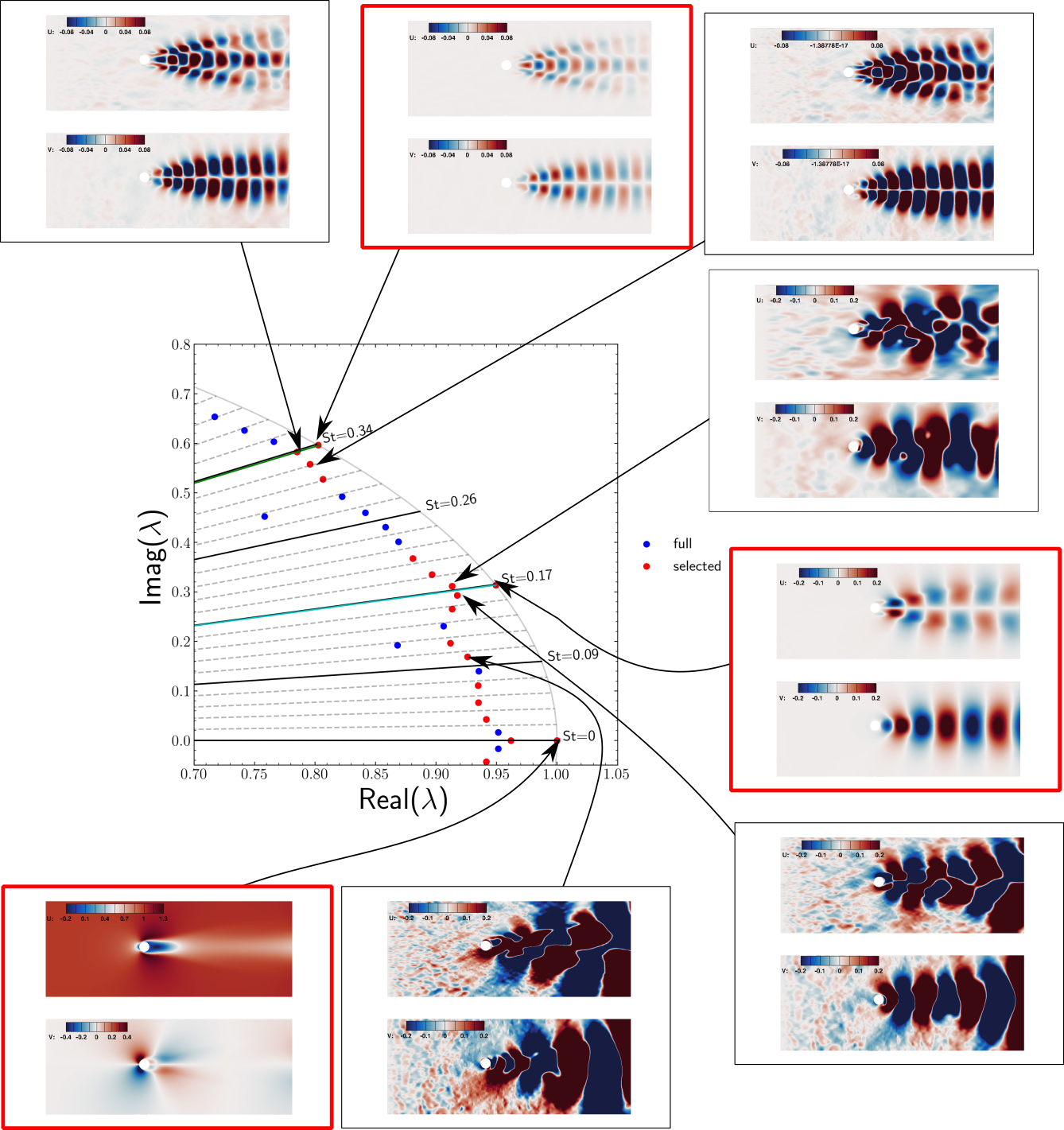
Figure 23: Contours of Koopman modes of $\Rey=100$ cylinder wake flow at $t=0$. Red squares indicate stable modes.

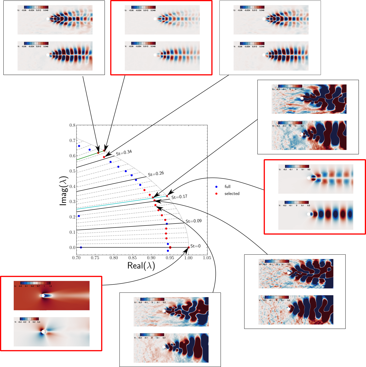
Figure 24: Contours of Koopman modes of $\Rey=130$ cylinder wake flow at $t=0$. Red squares indicate stable modes.

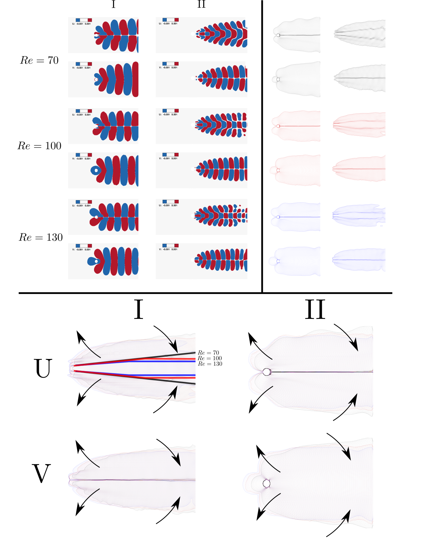
Figure 25: Top left: contribution of stable Koopman modes corresponding to type-I and type-II cluster for $\Rey=70,100,130$ at $t=0$ visualized with threshold 0.001. Top right: time-averaged iso-contour of top left plot. Bottom: tendency of “envelope” of type-I and II modes as $\Rey$ increases. Separation lines in $U$ component of type-I are drawn for $\Rey=70$ (black), $\Rey=100$ (red) and $\Rey=130$ (blue).

4.2.2 Net contribution of clustered Koopman modes

By examining figs. 22, 23 and 24, we observe that the colinearity of the spatial structures among each cluster can cause cancellations. A famous example of such non-oscillatory cancellation is the “shift mode” defined by Noack et al. (2003), in conjunction with two oscillating modes. As the “shift mode” decays, the stationary component of the flow transitions from the unstable equilibrium to the time-averaged mean. The existence of such non-oscillatory decaying Koopman modes is also confirmed by weakly non-linear analysis (Bagheri, 2013). Interestingly, our algorithm is able to identify not only the non-oscillatory cancellation (from the “shift mode”) but also oscillatory cancellations from two clusters with distinct frequencies. Such cancellations elegantly explain why no unstable Koopman eigenvalues appear in this flow given the co-existence of an attracting limit cycle and an unstable equilibrium. These modes could be understood as “oscillatory shift modes”, as a generalization of the model proposed by Noack et al. (2003).

Since modes within each cluster appear to be colinear to each other, it is intriguing to investigate the net contribution from each cluster. For the above $\Rey=70$ case, effects from different clusters for different time in the transient regime are shown in fig. 26. There are several interesting observations throughout the transient period from $t=80$ to $t=200$:

• The net contribution from “cluster 0” does not exhibit strong oscillations. For the contribution from “cluster 0 ”, the $U$ component shows a decrease in the length of the reverse flow region behind the cylinder with an increase in the low speed wake layer thickness while the $V$ component remains unchanged. This is similar to the effect of “shift mode” which also characterizes the decay of recirculation behind the cylinder.

• Initially at $t=80$, the net contribution from “cluster $I$” is rather weak primarily due to the “cancellation” from the lagged phase. Further, the development of vortex shedding downstream from the top and bottom surfaces of the cylinder is nearly parallel. This corresponds to the initial wiggling of the low speed wake flow downstream. As time increases, the pattern of corresponding vortices develops away from the center line.

• Although the net contribution from “cluster 0+$I$” captures most of the flow features from “full modes” throughout the transient regime, with increasing time, the net contribution from “cluster $II$” becomes more important and contributes to the strength of vortex shedding downstream.

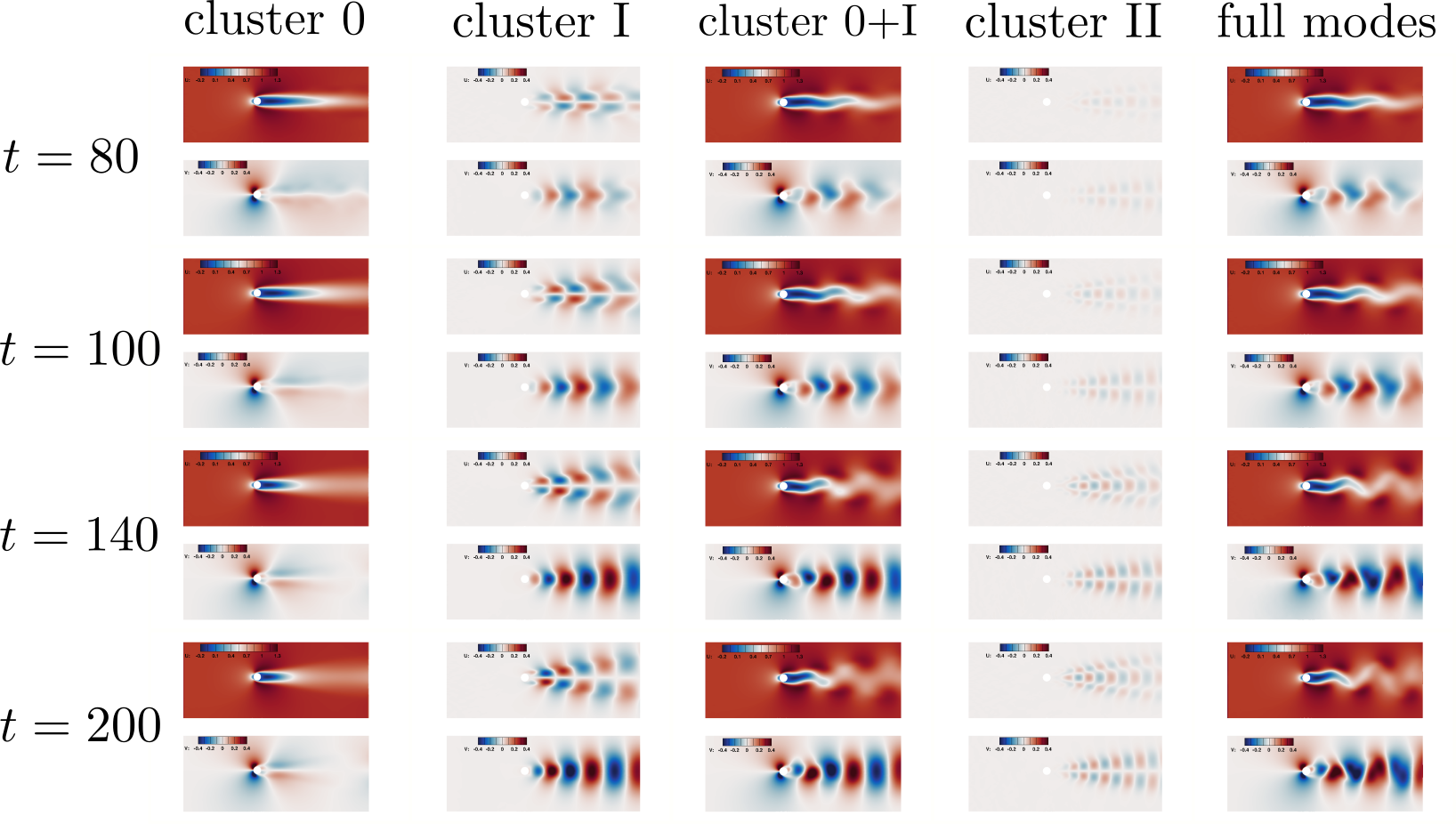
Figure 26: Contribution of Koopman modes at cluster level in the transient regime of $Re=70$ case. “cluster 0” denotes the cluster near the real axis in fig. 21. “cluster $I$” /“cluster $II$” takes the effect of mirror cluster in fourth quadrant into account. “full modes” denotes the aggregated contribution of Koopman modes.

4.2.3 Comparison with DMD and sparsity-promoting DMD at $\Rey=70$

To confirm the advantage of sparsity-promoting KDMD over DMD (Schmid, 2010) and spDMD (Jovanović et al., 2014), we compare the following three models on the unsteady cylinder wake flow at $\Rey=70$:

1. sparsity-promoting KDMD on top 20 POD coefficients with 34 modes selected,

2. DMD on top 20 POD coefficients,

3. spDMD  on top 200 POD coefficients with $\alpha$ chosen carefully such that only 34 modes are selected.

Note that DMD with top 200 POD coefficients, i.e., $r=200$ in SVD-DMD (Schmid, 2010), contains 10 times stable/decaying harmonics as DMD on the top 20 modes. Hence, it is not surprising to expect that the corresponding prediction of the evolution of the top 20 POD coefficients to be very good (not shown for clarity). However, to make a fair comparison against sparsity-promoting KDMD, we consider spDMD (Jovanović et al., 2014) on the top 200 POD coefficients with 34 modes selected.

As shown in fig. 27, given the same number of eigenmodes, sparsity-promoting KDMD performs remarkably better than spDMD, especially in the transient regime. This is likely due to the inability of DMD in capturing non-linear algebraic growth in the transient regime (Bagheri, 2013). spDMD overestimates the growth in $x_{1}$ and $x_{2}$ while ignoring a turnaround near the onset of transient regime in $x_{5}$ and $x_{8}$. As expected, DMD with 20 POD coefficients performs the worst especially for the modes where transient effects are dominant. Given the results in fig. 27, among all of the top 8 POD coefficients, $x_{6}$ and $x_{7}$ appear to be most challenging to model: DMD and spDMD cannot match the limit-cycle while spKDMD performs very well. Notice that the frequency in $x_{6}$ and $x_{7}$ corresponds to $St_{D}$. Hence, there will be a difference in predicting the fluctuation of $C_{D}$ between spDMD and sparsity-promoting KDMD.

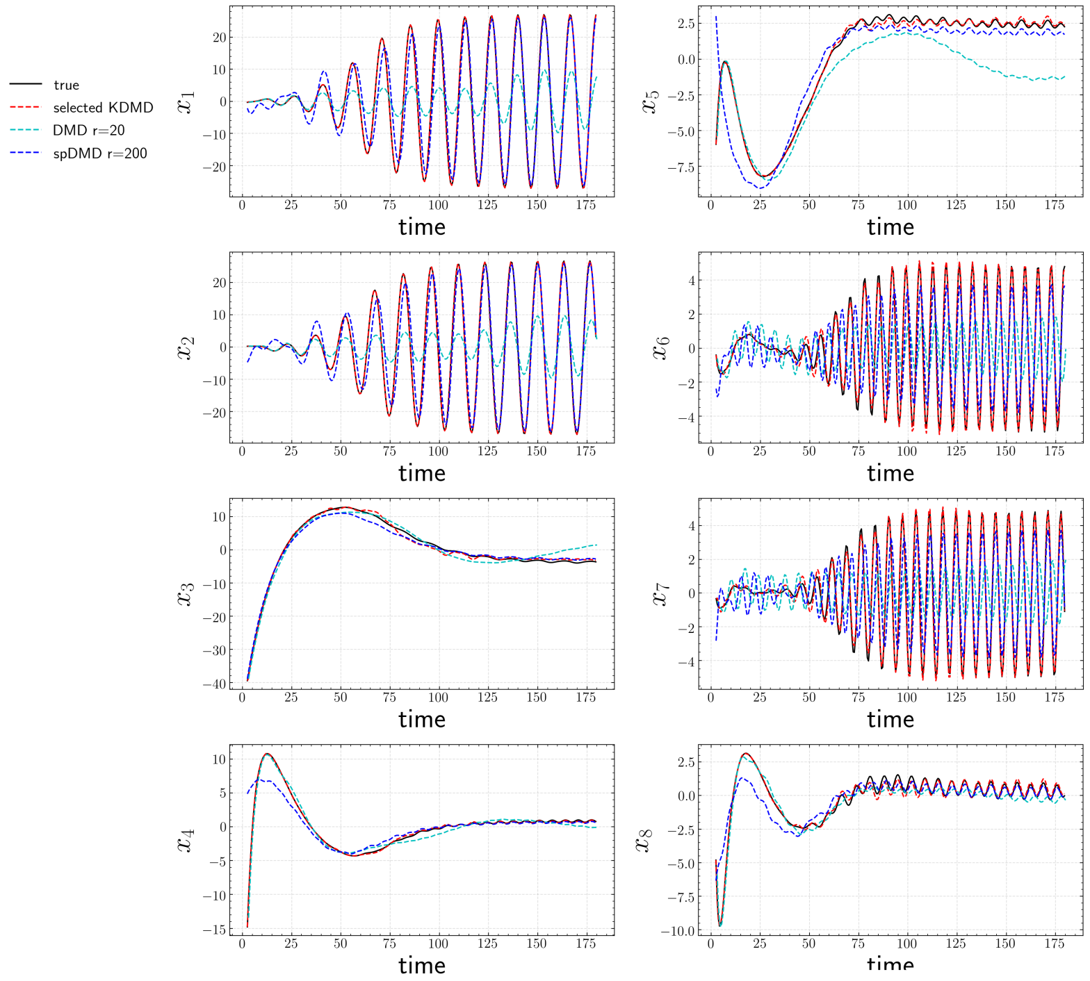
Figure 27: Comparison of a posteriori prediction on the top 8 POD coefficients of the testing trajectory between sparsity-promoting KDMD, DMD (Schmid, 2010) and spDMD (Jovanović et al., 2014) for the 2D cylinder flow at $\Rey=70$. $x_{i}$ denotes $i$-th POD coefficient.

Finally, comparison of the identified Koopman eigenvalues between DMD, spDMD and spKDMD is shown in fig. 28. On one hand, both spDMD and spKDMD exactly capture the stable eigenmodes that correspond to $St_{D}$ and $St_{L}$. This is expected since DMD with 200 POD coefficients represents the dynamics very well, and deviation from limit-cycle behavior would be penalized in spDMD. On the other hand, several erroneous stable DMD modes are obtained by DMD. This explains the deviation of a posteriori prediction from the ground truth limit cycle in fig. 27. For those decaying modes, similarity/co-linearity is observed between two clusters of eigenvalue from spDMD and spKDMD. However, spKDMD contains more high frequency modes than spDMD. Finally, it is interesting to note that, although the correct stable eigenvalues are captured accurately by both spDMD and spKDMD, the former does not capture accurate amplitudes for stable eigenvalues of type-II as seen in fig. 27.

As a side note, when the temporal mean was used instead of maximal error in the definition of $Q$ in eq. 29, spKDMD with the above setting was found to not find a stable eigenvalue corresponding to $ST_{D}$.

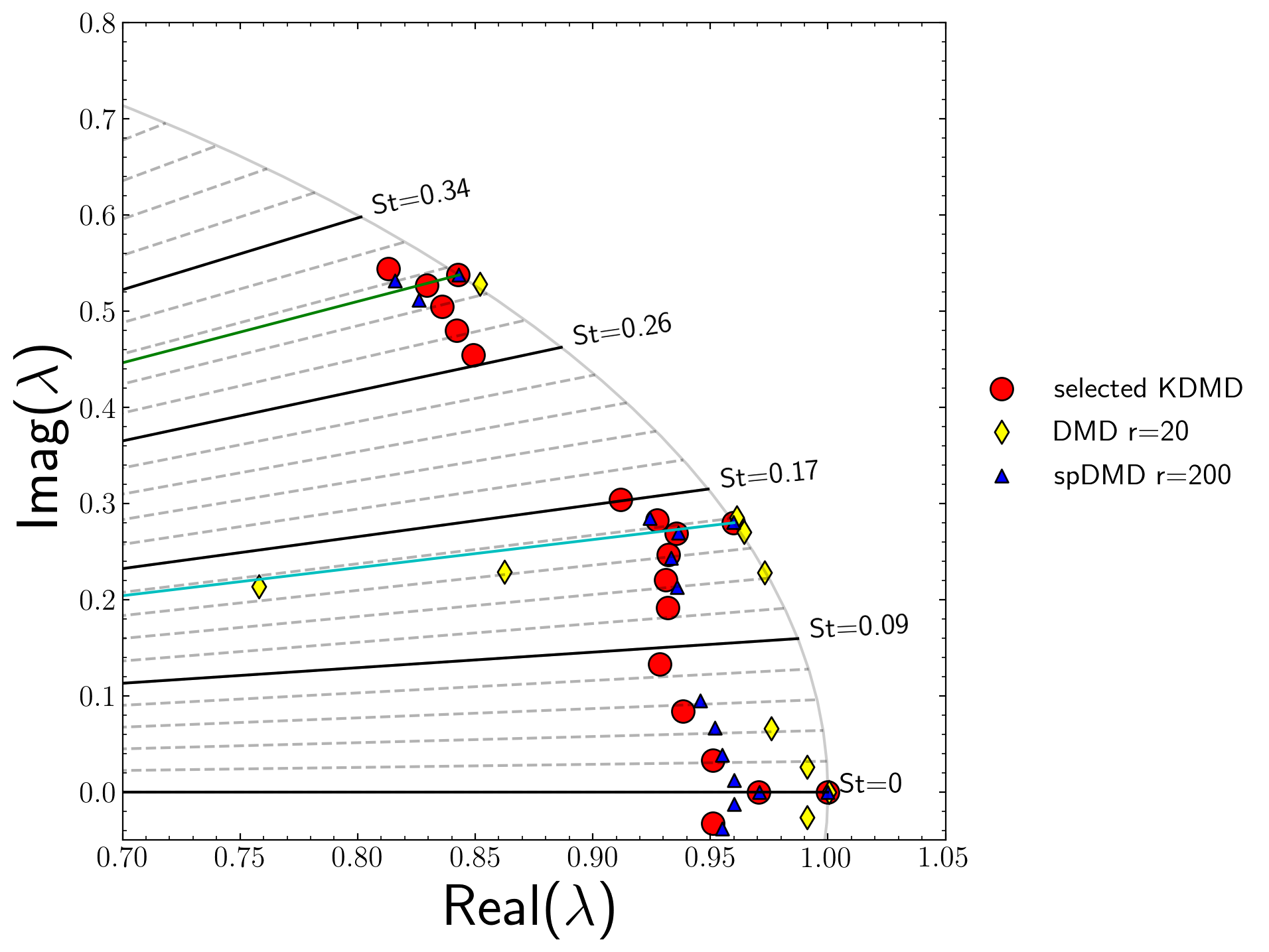
Figure 28: Comparison of identified eigenvalues between spKDMD, DMD (Schmid, 2010) and spDMD (Jovanović et al., 2014) for the 2D cylinder flow at $\Rey=70$

4.3 Three-dimensional transient turbulent ship airwake

Understanding unsteady ship airwake flows is critical to design safe shipboard operations, such as takeoff and landing of fixed or rotary wing aircraft (Forrest & Owen, 2010), especially when the wind direction becomes stochastic. Here we obtain snapshots from an unsteady Reynolds Averaged Navier–Stokes (URANS) simulation of a ship airwake using FLUENT (Ansys, 2016) with the shear layer corrected $k$-$\omega$ two-equation turbulence model. Unsteadiness arises from both bluff-body separation, and an abrupt change in wind direction. We consider a conceptual ship geometry called simple frigate shape 2 (SFS2). For the details of the geometry, readers are referred to (Yuan et al., 2018). Configuration of the simulation setup is shown in fig. 29 where $\alpha_{\infty}$ denotes the angle of side wind.

To prepare a proper initial condition, a URANS simulation for $U_{\infty}=15\mathrm{m/s}$ with $\alpha_{\infty}=0^{\circ}$, i.e., no side wind, is conducted to reach a physical initial condition. Following this, the last snapshot is used as the initial condition for a new run with an impulsive change in the wind direction from $\alpha_{\infty}=0^{\circ}$ to $\alpha_{\infty}=\alpha_{0}=5^{\circ}$. The boundary conditions for outlet/input is pressure outlet/velocity inlet while top and bottom are set as symmetry for simplicity. No-slip conditions are used at surface of the ship. Further details on the simulation setup are provided in (Sharma et al., 2019).

The sampling time interval is $\Delta t=0.1\mathrm{s}$ with 500 consecutive samples of the three velocity components. This corresponds to several flow through times over the ship length. The domain of interest is a cartesian region of mesh size $24\times 40\times 176$ starting on the rear landing deck. For dimension reduction, the trajectory of the top 40 POD coefficients (temporal mean subtracted) are collected, yielding $>99\%$ kinetic energy preservation. Discrete-time KDMD with an isotropic Gaussian kernel is employed to perform nonlinear Koopman analysis where $\sigma=200$, $r=135$ is chosen. Details of hyperparameter selection are provided in section C.3.

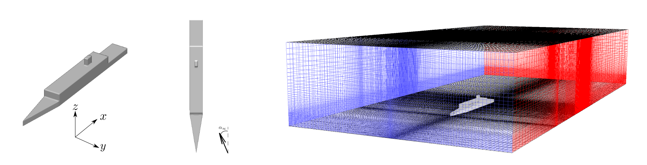
Figure 29: Left: geometry of the ship (SFS2). Right: generated computational mesh.

4.3.1 Results of discrete-time KDMD with mode selection

First, the error analysis of eigenfunctions is shown in fig. 30, where we choose $\hat{L}\approx 60$ for good reconstruction. However, the level of deviation from linear evolution is around 10%. This error will be reflected later as deviation in a posteriori prediction on the testing trajectory.

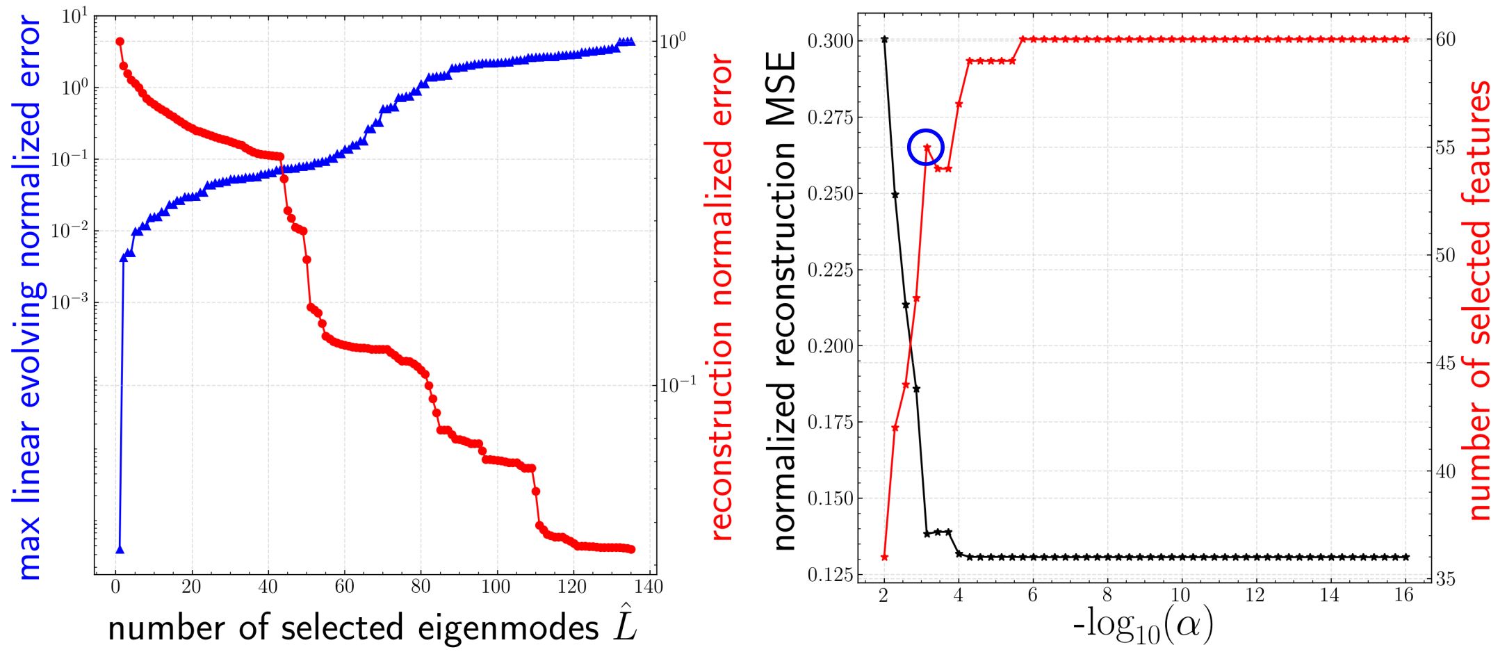
Figure 30: Left: Trend of linearly evolving error $Q$ and reconstruction error $R$ from discrete-time KDMD for the ship airwake. Right: Trend of linearly evolving error $Q$ and reconstruction error $R$ from discrete-time KDMD.

Second, the result of mode selection is summarized in table 3. Note that nearly 2/3 modes are removed. Furthermore, model performance in terms of a posteriori prediction on the testing trajectory is evaluated. Comparison between KDMD and the ground truth on contours of velocity components on a special $z-$plane (1.2 meters above the landing deck) is shown in fig. 31. Effects of an impulse change in wind direction in the following are observed from $t=1.5s$ to $t=30s$ and well-captured by spKDMD:

• growth of a large shear layer in $U$ on the rear (left) side of the superstructure on the ship

• a strong side wind sweep in $V$ above the landing deck propagating downstream

• development of vortex on the upwind (right) downstream side of the ship

$\alpha_{\textrm{select}}$	$7.19\times 10^{-4}$
number of selected modes	55
number of total modes	167
normalized reconstruction error $R$	0.133

Table 3: Summary of mode selection for discrete-time KDMD on ship airwake.

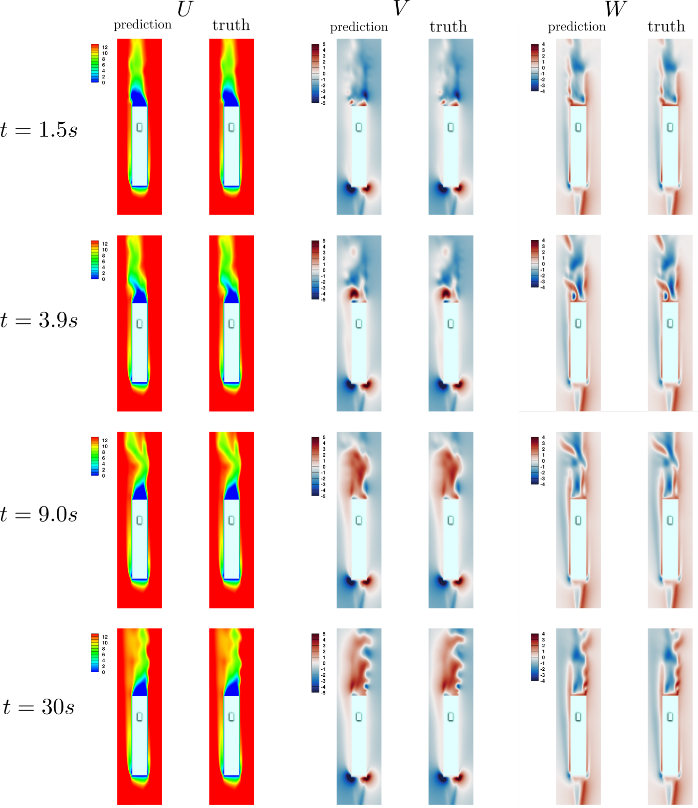
Figure 31: Contour of velocity components near the ship on $z-$plane slice at $t=1.5s$, 3.9s, 9.0s, 30s. For each subfigure, left: prediction from KDMD; right: ground truth.

Further, three velocity components of the Koopman mode decomposition on the previously mentioned $z-$plane is shown in fig. 32 together with the isocontour of vorticity colored by the velocity magnitude for the two stable harmonics. Note that frequency is normalized using $U_{\infty}$ as the reference velocity and funnel width of the ship $L=3.048\mathrm{m}$ as the characteristic length scale (Forrest & Owen, 2010). As expected, the spKDMD yields a large number of decaying modes with only three nontrivial stable harmonics, since significant transient effects are present in the data. From the Koopman mode decomposition in fig. 32, we observe the following:

• modes with eigenvalues close to each other exhibit similar spatial structure,

• modes associated with higher frequency are dominated by smaller scales,

• the stable harmonic mode near $St=0.09$ associated with a strong cone-shape vortex originating from the upwind (right) rear edge of the superstructure on the ship,

• the stable harmonic mode near $St=0.068$ corresponds to vortex shedding induced by the funnel,

• the slowly-decaying mode near $St=0.022$ shows unsteady circulation directly behind the superstructure,

• the steady mode ($St=0$) is consistent with the large circulation behind the superstructure, the roll-up wind on the side of landing deck, and vertical suction towards the floor on the landing deck.

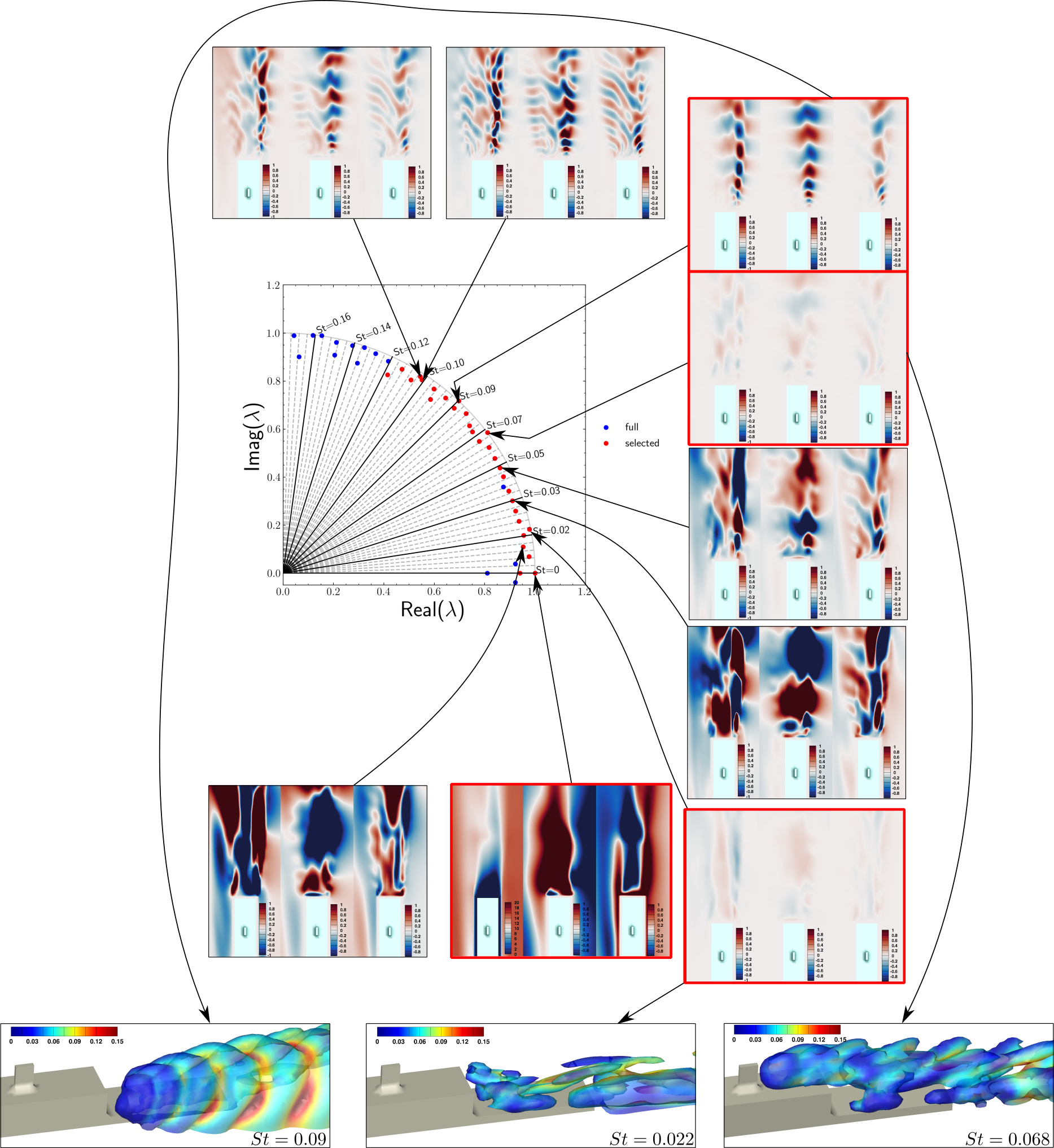
Figure 32: Contours of Koopman modes of ship airwake on the $z$-plane at $t=0$. For each subfigure, left: $U$, middle: $V$, right: $W$. Red squares indicate stable modes. Bottom: iso-contour of vorticity colored by velocity magnitude zoomed near the landing deck.

4.3.2 Comparison with sparsity-promoting DMD

We again repeat the comparison between our spKDMD and spDMD (Jovanović et al., 2014). Note that DMD on the first 40 POD modes performs poorly similar to section 4.2.3 and therefore not shown here. To make a fair comparison against the spKDMD from previous subsection, however, we collect the first 200 POD coefficients for spDMD to ensure that a sufficient number of modes are used to fit the trajectory well. We then carefully choose the penalty coefficient in spDMD to ensure that the same number of modes are retained as in spKDMD. As shown in fig. 33, within the time horizon $t<50$, a posteriori evaluation shows that spKDMD offers much improved predictions compared to spDMD (Jovanović et al., 2014) on the testing trajectory.

Moreover, as further illustrated in the left subfigure of fig. 34, eigenvalues identified from spKDMD only contain two stable modes while nearly all eigenvalues from spDMD are located near the unit circle, among which there are 30 out of 56 slightly unstable modes. These unstable modes inevitably lead to the identified system being numerically unstable when predicting beyond the current training time horizon, whereas spKDMD predicts a “physically consistent” limit cycle behavior. As indicated in the right subfigure of fig. 34, such instability is related to the inability of the (linear) features to approximate the Koopman-invariant subspace, where only 8 modes are within 10% of maximal deviation from linear evolution, compared to 60 modes in KDMD. We note that similar observations of the drastically different eigenvalue distribution were reported in the original KDMD paper (Williams et al., 2014).

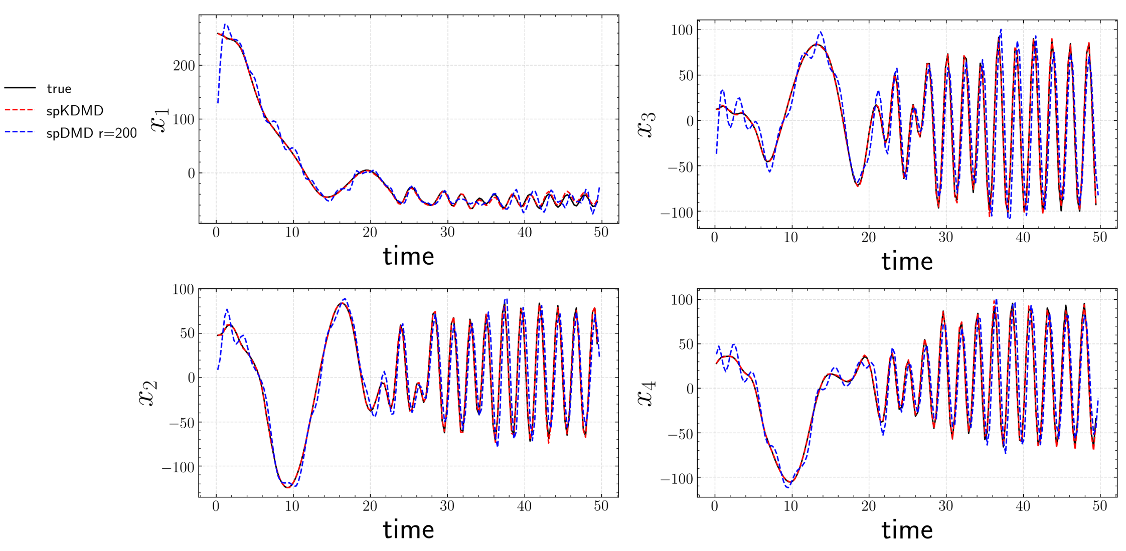
Figure 33: Comparison of a posteriori prediction of the 4 most significant POD coefficients of the testing trajectory between sparsity-promoting KDMD and spDMD (Jovanović et al., 2014) for the 3D ship-airwake flow. $x_{i}$ denotes $i$-th POD coefficient.

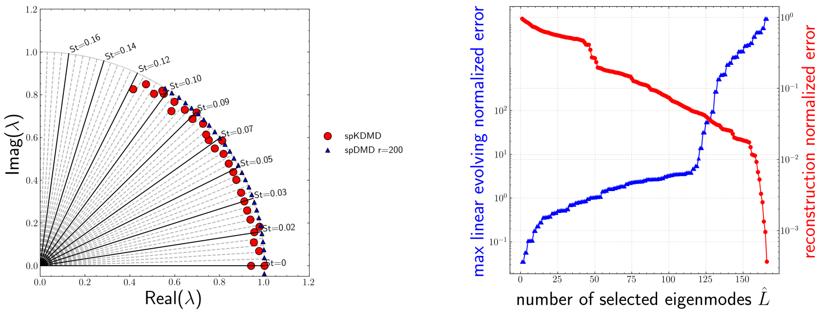
Figure 34: Left: Comparison of identified eigenvalues between spKDMD and spDMD (Jovanović et al., 2014) for the 3D ship-airwake flow. Right: Trend of linear evolving error $Q$ and reconstruction error $R$ from DMD for the 3D ship-airwake flow.

5 Conclusions

Two classical nonlinear approaches for the approximation of Koopman operator: EDMD and KDMD are revisited. From an algorithmic perspective, the main contributions of this work are a) Sparsity promoting techniques based on a posteriori error analysis, and b) multi-task learning techniques for mode selection as an extension of spDMD into the nonlinear variants. Further, analytical relationships between spDMD, Kou’s criterion and the proposed method are derived from the viewpoint of optimization. The algorithm  is first evaluated in detail on a simple two state dynamical system, for which the Koopman decomposition is known analytically.

If one is only interested in the post-transient dynamics of the system on an attractor, linear observables with time delays are sufficient to extract an informative Koopman-invariant subspace. Thus, the present techniques are evaluated on two fluid flows which involve strong transients: 2D flow over a cylinder at different Reynolds numbers, and a 3D ship airwake. We demonstrate the effectiveness of discovering accurate and informative Koopman-invariant subspaces from data and constructing accurate reduced order models from the viewpoint of Koopman theory. Furthermore, with the proposed algorithm, the parametric dependency of Koopman mode shapes on the Reynolds number is investigated for the cylinder flows. In this case, as $\Rey$ increases from 70 to 130, the shape of stable modes become flatter downstream and larger upstream. Moreover, the similarity of mode shapes between Koopman modes with similar eigenvalues is observed in both fluid flows. Specifically, five clusters of eigenvalues are observed in the case of 2D cylinder wake flow which is confirmed with weakly nonlinear theoretical analysis from Bagheri (2013). Type-I, II clusters are found to correspond to fluctuations in lift and drag respectively. We identify non-oscillatory as well as oscillatory cancellations from the above two clusters with distinct frequencies. These modes could be understood as “oscillatory shift modes”, as a generalization of the model proposed by Noack et al. (2003). For the 3D ship airwake case, two stable modes, and one slowly-decaying mode with distinct frequencies and mode shapes resulting from vortex shedding are extracted, and accurate predictive performance is observed in the transient regime.

Declaration of interests

The authors report no conflict of interest.

Appendix A Proof for the identity for eq. 22

Consider the economy SVD of $\mathbf{A}^{{}^{\prime}}=\mathbf{U}\mathbf{S}\mathbf{V}^{\textrm{H}}$. Since the column space of $\mathbf{A}^{{}^{\prime}}$ spans the column space of $\mathbf{Z}_{r}$, there exists an invertible matrix $\mathbf{P}$ such that $\mathbf{Z}_{r}\mathbf{P}=\mathbf{U}$. Hence,

$$\mathbf{A}^{{}^{\prime}}\mathbf{Z}_{r}=\mathbf{V}\mathbf{S}\mathbf{U}^{\textrm{H}}\mathbf{Z}_{r}=\mathbf{V}\mathbf{S}\mathbf{P}^{\textrm{H}}\mathbf{Z}_{r}^{\textrm{H}}\mathbf{Z}_{r}=\mathbf{V}\mathbf{S}\mathbf{P}^{\textrm{H}},$$

and $((\mathbf{A}^{{}^{\prime}}\mathbf{Z}_{r})^{\textrm{H}}\mathbf{A}^{{}^{\prime}}\mathbf{Z}_{r})^{+}=(\mathbf{P}^{-1})^{\textrm{H}}\mathbf{S}^{-2}\mathbf{P}^{-1}$. Thus

$$\mathbf{A}^{{}^{\prime}}\mathbf{A}^{{}^{\prime}\textrm{H}}\mathbf{Z}_{r}(\mathbf{Z}^{\textrm{H}}_{r}\mathbf{A}^{{}^{\prime}}\mathbf{A}^{{}^{\prime}\textrm{H}}\mathbf{Z}_{r})^{+}=(\mathbf{U}\mathbf{S}\mathbf{V}^{\textrm{H}})(\mathbf{V}\mathbf{S}\mathbf{P}^{\textrm{H}})(\mathbf{P}^{-1})^{\textrm{H}}\mathbf{S}^{-2}\mathbf{P}^{-1}=\mathbf{U}\mathbf{P}^{-1}=\mathbf{Z}_{r}.$$

Appendix B Computational complexity

Computational cost of the proposed framework can be divided in three parts:

1. Distributed SVD

2. KDMD/EDMD algorithms

3. Multi-task feature learning with the parameter sweep (solving eq. 36 with different values of $\alpha$)

The computational complexity for each step in the algorithm is summarized in table 4, where $n$ is the dimension of the system state, $M$ is the number of snapshots in the training , $r$ is the rank of the reduced system after SVD, $\hat{L}$ is the user-defined cut off for “accurate” features, and $N_{iter}$ is the maximal number of iterations user-defined to achieve a residual threshold, e.g. $10^{-12}$.

As shown in the Table. 4, the theoretical computational complexity for multi-task ElasticNet with an $\alpha$ sweep is $O(N_{\alpha}N_{iter}\hat{L}^{2}r)$. Note that this is a worst case simply because - except for the first $\alpha$ - we reuse the previous optimal solution as the initial condition for the new objective function to start the iterative optimization process. Also, thanks to SVD-based dimension reduction, the cost scales linearly with the reduced system rank $r$. Moreover, the user-defined linearly evolving error truncation $\hat{L}$ helps reduce that complexity as well instead of scaling with the number of snapshots $M$. Lastly, there is a cubic theoretical complexity associated with the number of snapshots when applying KDMD. The number of snapshots in a typical high fidelity simulation is $O(10^{3})$. That is to say, $r<10^{3}$ and $\hat{L}<10^{3}$. We note that computational efficiency can be further improved, but this will be left for future work.

Step	Computational complexity
SVD (QR iteration with vectors)	$O(Mn^{2})$0(Dongarra et al., 2018)
KDMD	$O(M^{3})$
error evaluation & pruning	$O(M^{2}n)$
multi-task ElasticNet with a fixed penalty coef. $\alpha$	$O(N_{iter}\hat{L}^{2}r)$
multi-task ElasticNet with $N_{\alpha}$ coefs. (worst case)	$O(N_{\alpha}N_{iter}\hat{L}^{2}r)$

Table 4: Computational complexity of each step in the proposed sparsity-promoting framework.

Appendix C Hyperparameter selection

C.1 2D fixed point attractor

We perform grid search in parallel for the selection of $\sigma$ and the truncated rank $r$ over the range: $\sigma\in[10^{-1},10]$ with 80 points uniformly distributed in the log sense and $r=36,50,70$ to find a proper combination of $r$ and $\sigma$. As shown in fig. 35, the higher rank $r$ leads to larger number of linearly evolving eigenfunctions. Thus, it is more crucial to choose a proper scale $\sigma$ than $r$ from fig. 35. However, considering the simplicity of this problem, $\sigma=2$ and $r=36$ would suffice.

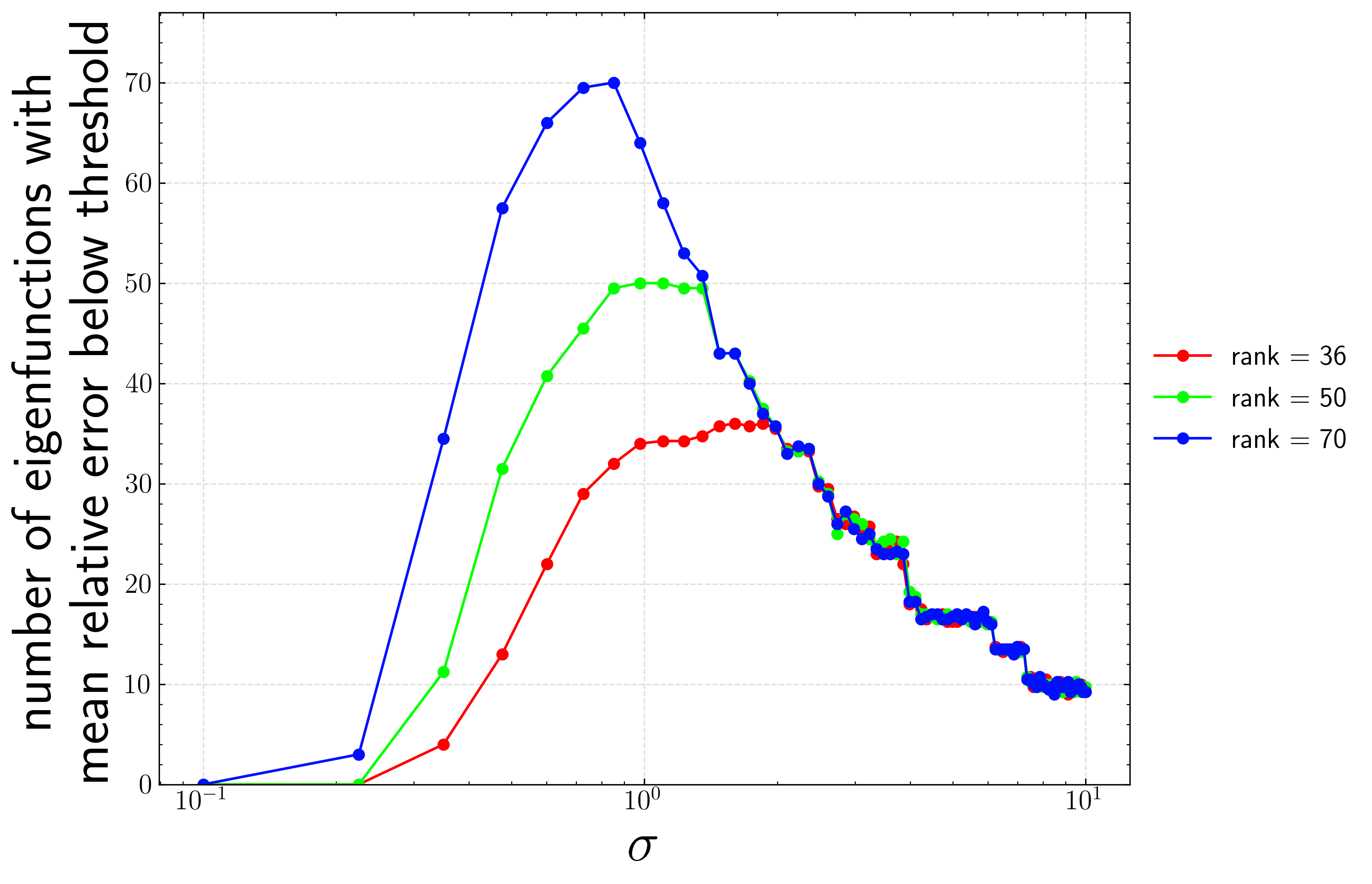
Figure 35: Hyperparameter search for isotropic Gaussian KDMD on the 2D fixed point attractor.

C.2 Cylinder flow case

As the flow is not turbulent, we choose hyperparameters for the $Re=70$ case and fix them for all the other cases. We sweep $\sigma$ from $[1,10^{5}]$ with 30 points uniformly distributed in the log sense and $r=120,140,160,180,200$ as shown in figure 36. From the plot, we choose $r=180$ and $\sigma=3$ for an approximate choice of the hyperparameter. Again, we observe that the number of accurate eigenfunctions first increases then decreases with $\sigma$ increasing and the saturation of rank truncation at higher $\sigma$ which is related to the variation in the characteristic scale of the features with respect to $\sigma$.

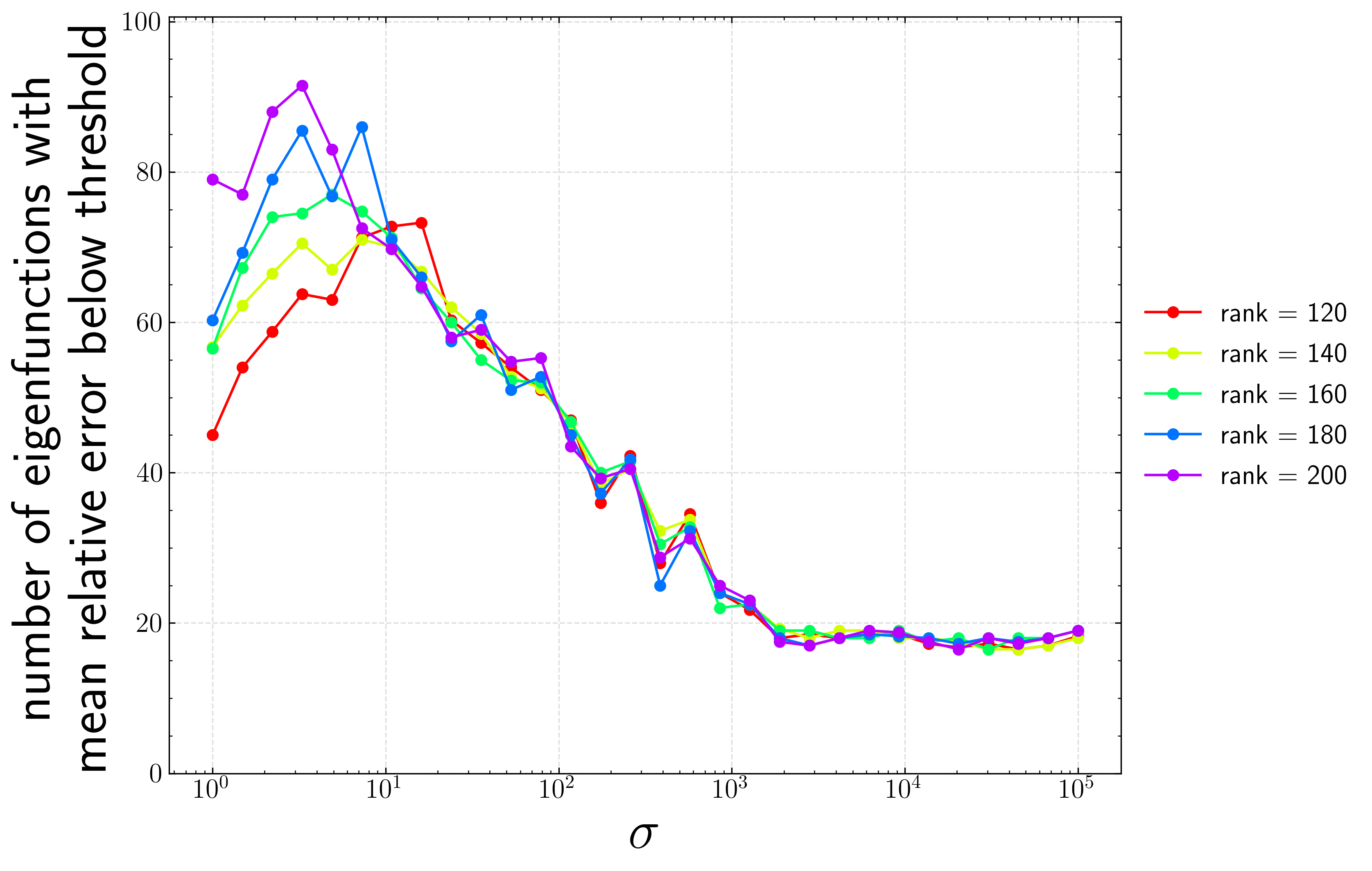
Figure 36: Hyperparameter search for isotropic Gaussian KDMD on transient cylinder wake flows.

C.3 Turbulent Ship-airwake case

Grid search in parallel for the selection of $\sigma$ and $r$ is performed over the range $\sigma\in[1,10^{5}]$ with 50 points uniformly distributed in the log sense, $r=40,80,120,130$. As shown in fig. 37, a good choice of $\sigma$ can be 200 for the case of $\alpha_{\infty}=5^{\circ}$. Note that since the hyperparameter selection is performed with a 5-fold cross validation on the training data, we only have up to $166*0.8\approx 132$ data points, i.e., maximal possible rank is 132. While in the actual training, we have maximal rank up to 166. Note that as long as the system is well-conditioned, the higher the rank, the richer the subspace. Here we take $\sigma=200$ and $r=135$.

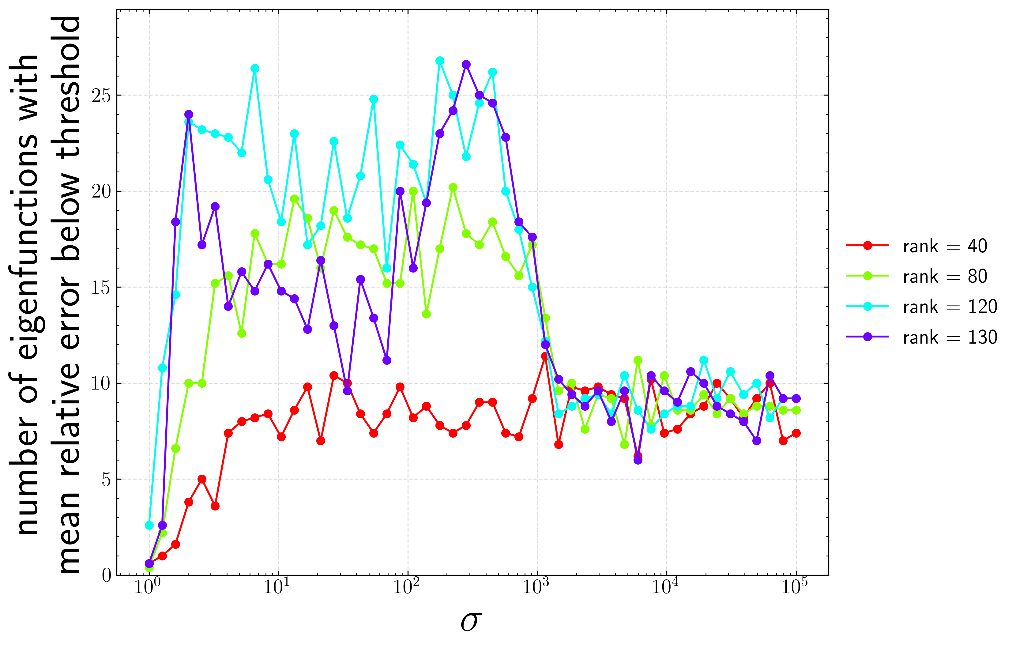
Figure 37: Hyperparameter search for isotropic Gaussian KDMD on transient ship airwake.

Appendix D Parallel Data Processing (PDP) Tool

The application of data-driven methodologies to increasingly large data sets has exposed the need for scalable tools. Method development is easily achieved in scripting environments, but for application to large multidimensional problems, memory and data I/O becomes a limiting factor. To illustrate this, consider a state-of-the art 3D computation. Given the fact that there are multiple variables associated with each grid cell, and that reasonable meshes can be expected to contain millions to hundreds of millions of cells, work-space memory requirements of Terabytes may be required. Utilizing available distributed tools and I/O strategies a generalized toolset, Parallel Data Processing(PDP), has been developed for application of complex methods to arbitrarily large data sets. Originally developed for use in reduced-order modeling, the generality of the toolset allows for a range of complex methodologies to applied. This is was leveraged for use in this work for the application of methods, as the problem size is intractable on desktop machines. The toolset leverages commonly available packages in the form of ScaLAPACK, PBLAS, and PBLACS Blackford et al. (1997) routines. ScaLAPACK is widely available on most computing resources where the original simulations are run.

References

- Ansys (2016) Ansys 2016 Ansys fluent user’s guide, release 17.0. Ansys .
- Arbabi et al. (2018) Arbabi, H, Korda, M & Mezic, I 2018 A data-driven koopman model predictive control framework for nonlinear flows (2018). arXiv preprint arXiv:1804.05291 .
- Arbabi & Mezić (2017a) Arbabi, Hassan & Mezić, Igor 2017a Ergodic theory, dynamic mode decomposition, and computation of spectral properties of the koopman operator. SIAM Journal on Applied Dynamical Systems 16 (4), 2096–2126.
- Arbabi & Mezić (2017b) Arbabi, Hassan & Mezić, Igor 2017b Study of dynamics in post-transient flows using koopman mode decomposition. Physical Review Fluids 2 (12), 124402.
- Argyriou et al. (2008a) Argyriou, Andreas, Evgeniou, Theodoros & Pontil, Massimiliano 2008a Convex multi-task feature learning. Machine Learning 73 (3), 243–272.
- Argyriou et al. (2008b) Argyriou, Andreas, Pontil, Massimiliano, Ying, Yiming & Micchelli, Charles A 2008b A spectral regularization framework for multi-task structure learning. In Advances in neural information processing systems, pp. 25–32.
- Aronszajn (1950) Aronszajn, Nachman 1950 Theory of reproducing kernels. Transactions of the American mathematical society 68 (3), 337–404.
- Askham & Kutz (2018) Askham, Travis & Kutz, J Nathan 2018 Variable projection methods for an optimized dynamic mode decomposition. SIAM Journal on Applied Dynamical Systems 17 (1), 380–416.
- Azencot et al. (2019) Azencot, Omri, Yin, Wotao & Bertozzi, Andrea 2019 Consistent dynamic mode decomposition. SIAM Journal on Applied Dynamical Systems 18 (3), 1565–1585.
- Bach et al. (2012) Bach, Francis, Jenatton, Rodolphe, Mairal, Julien, Obozinski, Guillaume & others 2012 Optimization with sparsity-inducing penalties. Foundations and Trends® in Machine Learning 4 (1), 1–106.
- Bagheri (2013) Bagheri, Shervin 2013 Koopman-mode decomposition of the cylinder wake. Journal of Fluid Mechanics 726, 596–623.
- Baudin et al. (2015) Baudin, M & others 2015 pydoe.
- Blackford et al. (1997) Blackford, L. S., Choi, J., Cleary, A., D’Azevedo, E., Demmel, J., Dhillon, I., Dongarra, J., Hammarling, S., Henry, G., Petitet, A., Stanley, K., Walker, D. & Whaley, R. C. 1997 ScaLAPACK Users’ Guide. Philadelphia, PA: Society for Industrial and Applied Mathematics.
- Bruce et al. (2019) Bruce, Adam L, Zeidan, Vera M & Bernstein, Dennis S 2019 What is the koopman operator? a simplified treatment for discrete-time systems. In 2019 American Control Conference (ACC), pp. 1912–1917. IEEE.
- Brunton et al. (2017) Brunton, Steven L, Brunton, Bingni W, Proctor, Joshua L, Kaiser, Eurika & Kutz, J Nathan 2017 Chaos as an intermittently forced linear system. Nature communications 8 (1), 19.
- Brunton et al. (2016a) Brunton, Steven L, Brunton, Bingni W, Proctor, Joshua L & Kutz, J Nathan 2016a Koopman invariant subspaces and finite linear representations of nonlinear dynamical systems for control. PloS one 11 (2), e0150171.
- Brunton et al. (2016b) Brunton, Steven L, Proctor, Joshua L & Kutz, J Nathan 2016b Discovering governing equations from data by sparse identification of nonlinear dynamical systems. Proceedings of the National Academy of Sciences 113 (15), 3932–3937.
- Budišić et al. (2012) Budišić, Marko, Mohr, Ryan & Mezić, Igor 2012 Applied koopmanism. Chaos: An Interdisciplinary Journal of Nonlinear Science 22 (4), 047510.
- Carlberg et al. (2013) Carlberg, Kevin, Farhat, Charbel, Cortial, Julien & Amsallem, David 2013 The gnat method for nonlinear model reduction: effective implementation and application to computational fluid dynamics and turbulent flows. Journal of Computational Physics 242, 623–647.
- Chen et al. (2012) Chen, Kevin K, Tu, Jonathan H & Rowley, Clarence W 2012 Variants of dynamic mode decomposition: boundary condition, koopman, and fourier analyses. Journal of nonlinear science 22 (6), 887–915.
- Cho & Saul (2009) Cho, Youngmin & Saul, Lawrence K 2009 Kernel methods for deep learning. In Advances in neural information processing systems, pp. 342–350.
- Dalcin et al. (2011) Dalcin, Lisandro D, Paz, Rodrigo R, Kler, Pablo A & Cosimo, Alejandro 2011 Parallel distributed computing using python. Advances in Water Resources 34 (9), 1124–1139.
- Dawson et al. (2016) Dawson, Scott TM, Hemati, Maziar S, Williams, Matthew O & Rowley, Clarence W 2016 Characterizing and correcting for the effect of sensor noise in the dynamic mode decomposition. Experiments in Fluids 57 (3), 42.
- DeGennaro & Urban (2019) DeGennaro, Anthony M & Urban, Nathan M 2019 Scalable extended dynamic mode decomposition using random kernel approximation. SIAM Journal on Scientific Computing 41 (3), A1482–A1499.
- Dongarra et al. (2018) Dongarra, Jack, Gates, Mark, Haidar, Azzam, Kurzak, Jakub, Luszczek, Piotr, Tomov, Stanimire & Yamazaki, Ichitaro 2018 The singular value decomposition: Anatomy of optimizing an algorithm for extreme scale. SIAM review 60 (4), 808–865.
- Dowell & Hall (2001) Dowell, Earl H & Hall, Kenneth C 2001 Modeling of fluid-structure interaction. Annual review of fluid mechanics 33 (1), 445–490.
- Drazin & Reid (2004) Drazin, Philip G & Reid, William Hill 2004 Hydrodynamic stability. Cambridge university press.
- Fey et al. (1998) Fey, Uwe, König, Michael & Eckelmann, Helmut 1998 A new strouhal–reynolds-number relationship for the circular cylinder in the range 47¡ re¡ 2 10 5. Physics of Fluids 10 (7), 1547–1549.
- Forrest & Owen (2010) Forrest, James S & Owen, Ieuan 2010 An investigation of ship airwakes using detached-eddy simulation. Computers & Fluids 39 (4), 656–673.
- Haseli & Cortés (2019) Haseli, Masih & Cortés, Jorge 2019 Efficient identification of linear evolutions in nonlinear vector fields: Koopman invariant subspaces. arXiv preprint arXiv:1909.01419 .
- Holmes et al. (2012) Holmes, Philip, Lumley, John L, Berkooz, Gahl & Rowley, Clarence W 2012 Turbulence, coherent structures, dynamical systems and symmetry. Cambridge university press.
- Hua et al. (2017) Hua, Jia-Chen, Noorian, Farzad, Moss, Duncan, Leong, Philip HW & Gunaratne, Gemunu H 2017 High-dimensional time series prediction using kernel-based koopman mode regression. Nonlinear Dynamics 90 (3), 1785–1806.
- Huang et al. (2018) Huang, Cheng, Duraisamy, Karthik & Merkle, Charles 2018 Challenges in reduced order modeling of reacting flows. In 2018 Joint Propulsion Conference, p. 4675.
- Jasak et al. (2007) Jasak, Hrvoje, Jemcov, Aleksandar, Tukovic, Zeljko & others 2007 Openfoam: A c++ library for complex physics simulations. In International workshop on coupled methods in numerical dynamics, , vol. 1000, pp. 1–20. IUC Dubrovnik Croatia.
- Jones et al. (2001–) Jones, Eric, Oliphant, Travis, Peterson, Pearu & others 2001– SciPy: Open source scientific tools for Python.
- Jovanović et al. (2014) Jovanović, Mihailo R, Schmid, Peter J & Nichols, Joseph W 2014 Sparsity-promoting dynamic mode decomposition. Physics of Fluids 26 (2), 024103.
- Jungers & Tabuada (2019) Jungers, Raphaël M & Tabuada, Paulo 2019 Non-local linearization of nonlinear differential equations via polyflows. In 2019 American Control Conference (ACC), pp. 1–6. IEEE.
- Kaiser et al. (2017) Kaiser, Eurika, Kutz, J Nathan & Brunton, Steven L 2017 Data-driven discovery of koopman eigenfunctions for control. arXiv preprint arXiv:1707.01146 .
- Kamb et al. (2018) Kamb, Mason, Kaiser, Eurika, Brunton, Steven L & Kutz, J Nathan 2018 Time-delay observables for koopman: Theory and applications. arXiv preprint arXiv:1810.01479 .
- Koopman (1931) Koopman, Bernard O 1931 Hamiltonian systems and transformation in hilbert space. Proceedings of the National Academy of Sciences of the United States of America 17 (5), 315.
- Korda & Mezić (2018a) Korda, Milan & Mezić, Igor 2018a Linear predictors for nonlinear dynamical systems: Koopman operator meets model predictive control. Automatica 93, 149–160.
- Korda & Mezić (2018b) Korda, Milan & Mezić, Igor 2018b On convergence of extended dynamic mode decomposition to the koopman operator. Journal of Nonlinear Science 28 (2), 687–710.
- Kou & Zhang (2017) Kou, Jiaqing & Zhang, Weiwei 2017 An improved criterion to select dominant modes from dynamic mode decomposition. European Journal of Mechanics-B/Fluids 62, 109–129.
- Kutz et al. (2016) Kutz, J Nathan, Brunton, Steven L, Brunton, Bingni W & Proctor, Joshua L 2016 Dynamic mode decomposition: data-driven modeling of complex systems. SIAM.
- Le Clainche & Vega (2017) Le Clainche, Soledad & Vega, José M 2017 Higher order dynamic mode decomposition. SIAM Journal on Applied Dynamical Systems 16 (2), 882–925.
- Li et al. (2017) Li, Qianxiao, Dietrich, Felix, Bollt, Erik M & Kevrekidis, Ioannis G 2017 Extended dynamic mode decomposition with dictionary learning: A data-driven adaptive spectral decomposition of the koopman operator. Chaos: An Interdisciplinary Journal of Nonlinear Science 27 (10), 103111.
- Lietz et al. (2017) Lietz, Amanda M, Johnsen, Eric & Kushner, Mark J 2017 Plasma-induced flow instabilities in atmospheric pressure plasma jets. Applied Physics Letters 111 (11), 114101.
- Lusch et al. (2018) Lusch, Bethany, Kutz, J Nathan & Brunton, Steven L 2018 Deep learning for universal linear embeddings of nonlinear dynamics. Nature communications 9 (1), 4950.
- Mamakoukas et al. (2019) Mamakoukas, Giorgos, Castano, Maria L, Tan, Xiaobo & Murphey, Todd 2019 Local koopman operators for data-driven control of robotic systems. In Robotics: science and systems.
- Mercer (1909) Mercer, J 1909 Functions of positive and negative type and their connection with the theory of integral equations, philosophical transsaction of the royal society of london, ser.
- Mezić (2005) Mezić, Igor 2005 Spectral properties of dynamical systems, model reduction and decompositions. Nonlinear Dynamics 41 (1-3), 309–325.
- Mezić (2013) Mezić, Igor 2013 Analysis of fluid flows via spectral properties of the koopman operator. Annual Review of Fluid Mechanics 45, 357–378.
- Minh (2010) Minh, Ha Quang 2010 Some properties of gaussian reproducing kernel hilbert spaces and their implications for function approximation and learning theory. Constructive Approximation 32 (2), 307–338.
- Noack et al. (2003) Noack, Bernd R, Afanasiev, Konstantin, MORZYŃSKI, MAREK, Tadmor, Gilead & Thiele, Frank 2003 A hierarchy of low-dimensional models for the transient and post-transient cylinder wake. Journal of Fluid Mechanics 497, 335–363.
- Otto & Rowley (2019) Otto, Samuel E & Rowley, Clarence W 2019 Linearly recurrent autoencoder networks for learning dynamics. SIAM Journal on Applied Dynamical Systems 18 (1), 558–593.
- Pan & Duraisamy (2018) Pan, Shaowu & Duraisamy, Karthik 2018 Long-time predictive modeling of nonlinear dynamical systems using neural networks. Complexity 2018.
- Pan & Duraisamy (2019) Pan, Shaowu & Duraisamy, Karthik 2019 On the structure of time-delay embedding in linear models of non-linear dynamical systems. arXiv preprint arXiv:1902.05198 .
- Pan & Duraisamy (2020) Pan, Shaowu & Duraisamy, Karthik 2020 Physics-informed probabilistic learning of linear embeddings of nonlinear dynamics with guaranteed stability. SIAM Journal on Applied Dynamical Systems 19 (1), 480–509.
- Parikh et al. (2014) Parikh, Neal, Boyd, Stephen & others 2014 Proximal algorithms. Foundations and Trends® in Optimization 1 (3), 127–239.
- Parish et al. (2020) Parish, Eric J, Wentland, Christopher R & Duraisamy, Karthik 2020 The adjoint petrov–galerkin method for non-linear model reduction. Computer Methods in Applied Mechanics and Engineering 365, 112991.
- Parry (2004) Parry, William 2004 Topics in ergodic theory, , vol. 75. Cambridge university press.
- Pedregosa et al. (2011) Pedregosa, F., Varoquaux, G., Gramfort, A., Michel, V., Thirion, B., Grisel, O., Blondel, M., Prettenhofer, P., Weiss, R., Dubourg, V., Vanderplas, J., Passos, A., Cournapeau, D., Brucher, M., Perrot, M. & Duchesnay, E. 2011 Scikit-learn: Machine learning in Python. Journal of Machine Learning Research 12, 2825–2830.
- Pope (2001) Pope, Stephen B 2001 Turbulent flows.
- Rasmussen (2003) Rasmussen, Carl Edward 2003 Gaussian processes in machine learning. In Summer School on Machine Learning, pp. 63–71. Springer.
- Röjsel (2017) Röjsel, Jimmy 2017 Koopman mode analysis of the side-by-side cylinder wake. Tech. Rep.. Royal Institute of Technology, Department of Mechanics.
- Rowley & Dawson (2017) Rowley, Clarence W & Dawson, Scott TM 2017 Model reduction for flow analysis and control. Annual Review of Fluid Mechanics 49, 387–417.
- Rowley et al. (2009) Rowley, Clarence W, Mezić, Igor, Bagheri, Shervin, Schlatter, Philipp & Henningson, Dan S 2009 Spectral analysis of nonlinear flows. Journal of fluid mechanics 641, 115–127.
- Schmid (2007) Schmid, Peter J 2007 Nonmodal stability theory. Annu. Rev. Fluid Mech. 39, 129–162.
- Schmid (2010) Schmid, Peter J 2010 Dynamic mode decomposition of numerical and experimental data. Journal of fluid mechanics 656, 5–28.
- Schmid et al. (2012) Schmid, Peter J, Violato, Daniele & Scarano, Fulvio 2012 Decomposition of time-resolved tomographic piv. Experiments in Fluids 52 (6), 1567–1579.
- Sharma et al. (2019) Sharma, Abhinav, Xu, Jiayang, Padthe, Ashwani K, Friedmann, Peretz P & Duraisamy, Karthik 2019 Simulation of maritime helicopter dynamics during approach to landing with time-accurate wind-over-deck. In AIAA Scitech 2019 Forum, p. 0861.
- Taira et al. (2019) Taira, Kunihiko, Hemati, Maziar S, Brunton, Steven L, Sun, Yiyang, Duraisamy, Karthik, Bagheri, Shervin, Dawson, Scott TM & Yeh, Chi-An 2019 Modal analysis of fluid flows: Applications and outlook. AIAA Journal pp. 1–25.
- Takeishi et al. (2017) Takeishi, Naoya, Kawahara, Yoshinobu & Yairi, Takehisa 2017 Learning koopman invariant subspaces for dynamic mode decomposition. In Advances in Neural Information Processing Systems, pp. 1130–1140.
- Tissot et al. (2014) Tissot, Gilles, Cordier, Laurent, Benard, Nicolas & Noack, Bernd R 2014 Model reduction using dynamic mode decomposition. Comptes Rendus Mécanique 342 (6-7), 410–416.
- Tu et al. (2013) Tu, Jonathan H, Rowley, Clarence W, Luchtenburg, Dirk M, Brunton, Steven L & Kutz, J Nathan 2013 On dynamic mode decomposition: theory and applications. arXiv preprint arXiv:1312.0041 .
- Wang et al. (2019) Wang, Linyu, Wang, Junyan, Xiang, Jianhong & hui Yue, Hui 2019 A re-weighted smoothed l 0-norm regularized sparse reconstructed algorithm for linear inverse problems. Journal of Physics Communications .
- White & Corfield (2006) White, Frank M & Corfield, Isla 2006 Viscous fluid flow, , vol. 3. McGraw-Hill New York.
- Williams et al. (2015) Williams, Matthew O, Kevrekidis, Ioannis G & Rowley, Clarence W 2015 A data–driven approximation of the koopman operator: Extending dynamic mode decomposition. Journal of Nonlinear Science 25 (6), 1307–1346.
- Williams et al. (2014) Williams, Matthew O, Rowley, Clarence W & Kevrekidis, Ioannis G 2014 A kernel-based approach to data-driven koopman spectral analysis. arXiv:1411.2260 .
- Xu & Duraisamy (2019) Xu, Jiayang & Duraisamy, Karthik 2019 Multi-level convolutional autoencoder networks for parametric prediction of spatio-temporal dynamics. arXiv preprint arXiv:1912.11114 .
- Xu et al. (2020) Xu, Jiayang, Huang, Cheng & Duraisamy, Karthik 2020 Reduced-order modeling framework for combustor instabilities using truncated domain training. AIAA Journal 58 (2), 618–632.
- Yeung et al. (2019) Yeung, Enoch, Kundu, Soumya & Hodas, Nathan 2019 Learning deep neural network representations for koopman operators of nonlinear dynamical systems. In 2019 American Control Conference (ACC), pp. 4832–4839. IEEE.
- Yuan et al. (2018) Yuan, Weixing, Wall, Alanna & Lee, Richard 2018 Combined numerical and experimental simulations of unsteady ship airwakes. Computers & Fluids 172, 29–53.
- Zhang et al. (2017) Zhang, Hao, Dawson, Scott, Rowley, Clarence W, Deem, Eric A & Cattafesta, Louis N 2017 Evaluating the accuracy of the dynamic mode decomposition. arXiv preprint arXiv:1710.00745 .
- Zhang & Schaeffer (2019) Zhang, Linan & Schaeffer, Hayden 2019 On the convergence of the sindy algorithm. Multiscale Modeling & Simulation 17 (3), 948–972.
- Zhao et al. (2015) Zhao, Liang, Sun, Qian, Ye, Jieping, Chen, Feng, Lu, Chang-Tien & Ramakrishnan, Naren 2015 Multi-task learning for spatio-temporal event forecasting. In Proceedings of the 21th ACM SIGKDD International Conference on Knowledge Discovery and Data Mining, pp. 1503–1512. ACM.
- Zou & Hastie (2005) Zou, Hui & Hastie, Trevor 2005 Regularization and variable selection via the elastic net. Journal of the royal statistical society: series B (statistical methodology) 67 (2), 301–320.