Three Approaches for Personalization with Applications to Federated Learning

Abstract

The standard objective in machine learning is to train a single model for all users. However, in many learning scenarios, such as cloud computing and federated learning, it is possible to learn a personalized model per user. In this work, we present a systematic learning-theoretic study of personalization. We propose and analyze three approaches: user clustering, data interpolation, and model interpolation. For all three approaches, we provide learning-theoretic guarantees and efficient algorithms for which we also demonstrate the performance empirically. All of our algorithms are model-agnostic and work for any hypothesis class.

1 Introduction

A popular application of language models is virtual keyboard applications, where the goal is to predict the next word, given the previous words (Hard et al., 2018). For example, given “I live in the state of”, ideally, it should guess the state the user intended to type. However, suppose we train a single model on all the user data and deploy it, then the model would predict the same state for all users and would not be a good model for most. Similarly, in many practical applications, the distribution of data across clients is highly non-i.i.d. and training a single global model for all clients may not be optimal.

Thus, we study the problem of learning personalized models, where the goal is to train a model for each client, based on the client’s own dataset and the datasets of other clients. Such an approach would be useful in applications with the natural infrastructure to deploy a personalized model for each client, which is the case with large-scale learning scenarios such as federated learning (FL) (McMahan et al., 2017).

Before we proceed further, we highlight one of our use cases in FL. In FL, typically a centralized global model is trained based on data from a large number of clients, which may be mobile phones, other mobile devices, or sensors (Konečnỳ et al., 2016b, a; McMahan et al., 2017; Yang et al., 2019) using a variant of stochastic gradient descent called FedAvg. This global model benefits from having access to client data and can often perform better on several learning problems, including next word prediction (Hard et al., 2018; Yang et al., 2018) and predictive models in health (Brisimi et al., 2018). We refer to Appendix A.1 for more details on FL.

Personalization of machine learning models has been studied extensively for specific applications such as speech recognition (Yu and Li, 2017). However, many algorithms are speech specific or not suitable for FL due to distributed constraints. Personalization is also related to Hierarchical Bayesian models (Gelman, 2006; Allenby et al., 2005). However, they are not directly applicable for FL. Personalization in the context of FL has been studied by several works via multi-task learning (Smith et al., 2017), meta-learning (Jiang et al., 2019; Khodak et al., 2019), use of local parameters (Arivazhagan et al., 2019; Liang et al., 2020), mixture of experts (Peterson et al., 2019), finetuning and variants (Wang et al., 2019; Yu et al., 2020) among others. We refer readers to Appendix A.2 for an overview of works on personalization in FL.

We provide a learning-theoretic framework, generalization guarantees, and computationally efficient algorithms for personalization. Since FL is one of the main frameworks where personalized models can be used, we propose efficient algorithms that take into account computation and communication bottlenecks.

2 Preliminaries

Before describing the mathematical details of personalization, we highlight two related models. The first one is the global model trained on data from all the clients. This can be trained using either standard empirical risk minimization (Vapnik, 1992) or other methods such as agnostic risk minimization (Mohri et al., 2019). The second baseline model is the purely local model trained only on the client’s data.

The global model is trained on large amounts of data and generalizes well on unseen test data; however it does not perform well for clients whose data distributions are very different from the global train data distribution. On the other hand, the train data distributions of local models match the ones at inference time, but they do not generalize well due to the scarcity of data.

Personalized models can be viewed as intermediate models between pure-local and global models. Thus, the hope is that they incorporate the generalization properties of the global model and the distribution matching property of the local model. Before we proceed further, we first introduce the notation used in the rest of the paper.

2.1 Notation

We start with some general notation and definitions used throughout the paper. Let ${\mathscr{X}}$ denote the input space and ${\mathscr{Y}}$ the output space. We will primarily discuss a multi-class classification problem where ${\mathscr{Y}}$ is a finite set of classes, but much of our results can be extended straightforwardly to regression and other problems. The hypotheses we consider are of the form $h\colon{\mathscr{X}}\to\Delta^{\mathscr{Y}}$, where $\Delta^{\mathscr{Y}}$ stands for the simplex over ${\mathscr{Y}}$. Thus, $h(x)$ is a probability distribution over the classes that can be assigned to $x\in{\mathscr{X}}$. We will denote by ${\mathscr{H}}$ a family of such hypotheses $h$. We also denote by $\ell$ a loss function defined over $\Delta^{\mathscr{Y}}\times{\mathscr{Y}}$ and taking non-negative values. The loss of $h\in{\mathscr{H}}$ for a labeled sample $(x,y)\in{\mathscr{X}}\times{\mathscr{Y}}$ is given by $\ell(h(x),y)$. Without loss of generality, we assume that the loss $\ell$ is bounded by one. We will denote by ${\mathscr{L}}_{\mathscr{D}}(h)$ the expected loss of a hypothesis $h$ with respect to a distribution ${\mathscr{D}}$ over ${\mathscr{X}}\times{\mathscr{Y}}$:

$${\mathscr{L}}_{\mathscr{D}}(h)=\operatorname*{\mathbb{E}}_{(x,y)\sim{\mathscr{D}}}[\ell(h(x),y)],$$

and by $h_{\mathscr{D}}$ its minimizer: $h_{\mathscr{D}}=\operatorname*{argmin}_{h\in{\mathscr{H}}}{\mathscr{L}}_{\mathscr{D}}(h)$. Let ${\mathfrak{R}}_{{{\mathscr{D}}},m}({\mathscr{H}})$ denote the Rademacher complexity of class ${\mathscr{H}}$ over the distribution ${{\mathscr{D}}}$ with $m$ samples.

Let $p$ be the number of clients. The distribution of samples of client $k$ is denoted by ${\mathscr{D}}_{k}$. Clients do not know the true distribution, but instead, have access to $m_{k}$ samples drawn i.i.d. from the distribution ${\mathscr{D}}_{k}$. We will denote by $\widehat{{\mathscr{D}}}_{k}$ the corresponding empirical distribution of samples and by $m=\sum^{p}_{k=1}m_{k}$ the total number of samples.

2.2 Local model

We first ask when it is beneficial for a client to participate in global model training. Consider a canonical user with distribution ${\mathscr{D}}_{1}$. Suppose we train a purely local model based on the client’s data and obtain a model $h_{\widehat{{\mathscr{D}}}_{1}}$. By standard learning-theoretic tools (Mohri et al., 2018), the performance of this model can be bounded as follows: with probability at least $1-\delta$, the minimizer of empirical risk ${\mathscr{L}}_{\widehat{{\mathscr{D}}}_{1}}(h)$ satisfies

$${\mathscr{L}}_{{\mathscr{D}}_{1}}(h_{\widehat{{\mathscr{D}}}_{1}})-{\mathscr{L}}_{{\mathscr{D}}_{1}}(h_{{\mathscr{D}}_{1}})=\mathcal{O}\left({\mathfrak{R}}_{{\mathscr{D}}_{1},m_{1}}({\mathscr{H}})\right)=\mathcal{O}\left(\frac{\sqrt{d+\log{1}/{\delta}}}{\sqrt{m_{1}}}\right),$$ (1)

where ${\mathfrak{R}}_{{\mathscr{D}}_{1},m_{1}}({\mathscr{H}})$ is the Rademacher complexity and $d$ is the pseudo-dimension of the hypothesis class ${\mathscr{H}}$ (Mohri et al., 2018). Note that pseudo-dimension coincides with VC dimension for $0-1$ loss. From (1), it is clear that local models perform well when the number of samples $m_{1}$ is large. However, this is often not the case. In many realistic settings, such as virtual keyboard models, the average number of samples per user is in the order of hundreds, whereas the pseudo-dimension of the hypothesis class is in millions (Hard et al., 2018). In such cases, the above bound becomes vacuous.

2.3 Uniform global model

The global model is trained by minimizing the empirical risk on the concatenation of all the samples. For $\lambda\in\Delta^{p}$, the weighted average distribution ${\mathscr{D}}_{\lambda}$ is given by $\sum_{k}\lambda_{k}{\mathscr{D}}_{k}$. The global model is trained on the concatenated samples from all the users and hence is equivalent to minimize the loss on the distribution $\hat{{\mathscr{U}}}=\sum_{k}\lambda^{\prime}_{k}\widehat{{\mathscr{D}}}_{k}$, where $\lambda^{\prime}_{k}=m_{k}/m$. Since the global model is trained on data from all the clients, it may not match the actual underlying client distribution and thus may perform worse.

The divergence between distributions is often measured by a Bregman divergence such as KL-divergence or unnormalized relative entropy. However, such divergences do not consider the underlying machine learning task at hand for example learning the best hypotheses out of ${\mathscr{H}}$. To obtain better bounds, we use the notion of label-discrepancy between distributions (Mansour et al., 2009b; Mohri and Medina, 2012). For two distributions over features and labels, ${\mathscr{D}}_{1}$ and ${\mathscr{D}}_{2}$, and a class of hypotheses $\mathcal{H}$, label-discrepancy(Mohri and Medina, 2012) is given by

$$\text{disc}_{\mathcal{H}}({\mathscr{D}}_{1},{\mathscr{D}}_{2})=\max_{h\in\mathcal{H}}|{\mathscr{L}}_{{\mathscr{D}}_{1}}(h)-{\mathscr{L}}_{{\mathscr{D}}_{2}}(h)|.$$

If the loss of all the hypotheses in the class is the same under both ${\mathscr{D}}_{1}$ and ${\mathscr{D}}_{2}$, then the discrepancy is zero and models trained on ${\mathscr{D}}_{1}$ generalize well on ${\mathscr{D}}_{2}$ and vice versa.

With the above definitions, it can be shown that the uniform global model generalizes as follows: with probability at least $1-\delta$, the minimizer of empirical risk on the uniform distribution satisfies

$${\mathscr{L}}_{{\mathscr{D}}_{1}}(h_{\hat{\mathscr{U}}})-{\mathscr{L}}_{{\mathscr{D}}_{1}}(h_{{\mathscr{D}}_{1}})=\mathcal{O}\left({\mathfrak{R}}_{{\mathscr{U}},m}({\mathscr{H}})\right)+\text{disc}_{\mathcal{H}}({\mathscr{D}}_{1},{\mathscr{U}})=\mathcal{O}\left(\frac{\sqrt{d+\log{1}/{\delta}}}{\sqrt{m}}\right)+\text{disc}_{\mathcal{H}}({\mathscr{D}}_{1},{\mathscr{U}}).$$ (2)

Since the global model is trained on the concatenation of all users’ data, it generalizes well. However, due to the distribution mismatch, the model may not perform well for a specific user. If ${{\mathscr{U}}}=\sum_{k}\lambda^{\prime}_{k}{{\mathscr{D}}}_{k}$, the difference between local and global models depends on the discrepancy between ${\mathscr{D}}_{1}$ and ${\mathscr{U}}$, $m_{1}$ the number of samples from the domain ${\mathscr{D}}_{1}$, and the total number of samples $m$. While in most practical applications $m_{1}$ is small and hence a global model usually performs better, this is not guaranteed. We provide a simple example illustrating such a case in Appendix B.1.

Since the uniform global model assigns weight $m_{k}/m$ to client $k$, clients with larger numbers of samples receive higher importance. This can adversely affect clients with small amounts of data. Furthermore, by (2), the model may not generalize well for clients whose distribution is different than the uniform distribution. Thus, (1) and (2) give some guidelines under which it is beneficial for clients to participate in global model training.

Instead of using uniform weighting of samples, one can use agnostic risk proposed by Mohri et al. (2019), which is more risk averse. We refer to Appendix B.2 for details about the agnostic risk minimization.

3 Our contributions

We ask if personalization can be achieved by an intermediate model between the local and global models. Furthermore, for ease of applicability and to satisfy the communication constraints in FL, we focus on scalable algorithms with low communication bottleneck. This gives rise to three natural algorithms, which are orthogonal and can be used separately or together.

• Train a model for subsets of users: we can cluster users into groups and train a model for each group. We refer to this as user clustering, or more refinely hypothesis-based clustering.

• Train a model on interpolated data: we can combine the local and global data and train a model on their combination. We refer to this as data interpolation.

• Combine local and global models: we can train a local and a global model and use their combination. We refer to this as model interpolation.

We provide generalization bounds and communication-efficient algorithms for all of the above methods. We show that the above three methods has small communication bottleneck and enjoys qualitative privacy benefits similar to training a global model. Of the three proposed approaches, data interpolation has non-trivial communication cost and data security. We show that data interpolation can be implemented with small communication overhead in Section 5. We also show discuss data security aspect and methods to improve it in Appendix D.3.

Of the remaining methods, model interpolation has the same communication cost and security as that of training a single model. Clustering has the same data security as that of training single models, but the communication cost is $q$ times that of training a single model, where $q$ is the number of clusters. In the rest of the paper, we study each of the above methods.

4 User clustering

Instead of training a single global model, a natural approach is to cluster clients into groups and train a model for each group. This is an intermediate model between a purely local and global model and provides a trade-off between generalization and distribution mismatch. If we have a clustering of users, then we can naturally find a model for each user using standard optimization techniques. In this section, we ask how to define clusters. Clustering is a classical problem with a broad literature and known algorithms (Jain, 2010). We argue that, since the subsequent application of our clustering is known, incorporating it into the clustering algorithm will be beneficial. We refer readers to Appendix C.1 for more details on comparison to baseline works.

4.1 Hypothesis-based clustering

Consider the scenario where we are interested in finding clusters of images for a facial recognition task. Suppose we are interested in finding clusters of users for each gender and find a good model for each cluster. If we naively use the Bregman divergence clustering, it may focus on clustering based on the image background e.g., outdoor or indoors to find clusters instead of gender.

To overcome this, we propose to incorporate the task at hand to obtain better clusters. We refer to this approach as hypothesis-based clustering and show that it admits better generalization bounds than the Bregman divergence approach. We partition users into $q$ clusters and find the best hypothesis for each cluster. In particular, we use the following optimization:

$$\min_{h_{1},\ldots,h_{q}}\sum^{p}_{k=1}\lambda_{k}\cdot\min_{i\in[q]}{\mathscr{L}}_{{\mathscr{D}}_{k}}(h_{i}),$$ (3)

where $\lambda_{k}$ is the importance of client $k$. The above loss function trains $q$ best hypotheses and naturally divides $\mathcal{X}\times\mathcal{Y}$ into $q$ partitions, where each partition is associated with a particular hypothesis $h_{k}$. In practice, we only have access to the empirical distributions $\widehat{{\mathscr{D}}}_{k}$. We replace ${\mathscr{L}}_{{\mathscr{D}}_{k}}(h_{i})$ by ${\mathscr{L}}_{\widehat{\mathscr{D}}_{k}}(h_{i})$ in optimization. To simplify the analysis, we use the fraction of samples from each user $m_{k}/m$ as $\lambda_{k}$. An alternative approach is to use $\lambda_{k}=1/p$ for all users, which assigns equal weight to all clients. The analysis is similar and we omit it to be concise.

4.2 Generalization bounds

We now analyze the generalization properties of this technique. We bound the maximum difference between true cluster based loss and empirical cluster based loss for all hypotheses. We note that such a generalization bound holds for any clustering algorithm (see Appendix C.2).

Let $C_{1},C_{2}\ldots,C_{q}$ be the clusters and let $m_{C_{i}}$ be the number of samples from cluster $i$. Let ${\mathscr{C}}_{i}$ and $\widehat{{\mathscr{C}}}_{i}$ be the empirical and true distributions of cluster ${\mathscr{C}}_{i}$. With these definitions, we now bound the generalization error of this technique.

Theorem 4.1 (Appendix C.3).

With probability at least $1-\delta$,

$$\max_{h_{1},\ldots,h_{q}}\left\lvert\sum^{p}_{k=1}\frac{m_{k}}{m}\cdot\left(\min_{i\in[q]}{\mathscr{L}}_{{\mathscr{D}}_{k}}(h_{i})-\min_{i\in[q]}{\mathscr{L}}_{\widehat{{\mathscr{D}}}_{k}}(h_{i})\right)\right\rvert\leq 2\sqrt{\frac{p\log\frac{2q}{\delta}}{m}}+\max_{C_{1},\ldots,C_{q}}\sum^{q}_{i=1}\frac{m_{C_{i}}}{m}{\mathfrak{R}}_{{\mathscr{C}}_{i},m_{C_{i}}}({\mathscr{H}}).$$

The above result implies the following corollary, which is easier to interpret.

Corollary 4.2 (Appendix C.4).

Let $d$ be the pseudo-dimension of ${\mathscr{H}}$. Then with probability at least $1-\delta$, the following holds:

$$\max_{h_{1},\ldots,h_{q}}\left\lvert\sum^{p}_{k=1}\frac{m_{k}}{m}\cdot\left(\min_{i\in[q]}{\mathscr{L}}_{{\mathscr{D}}_{k}}(h_{i})-\min_{i\in[q]}{\mathscr{L}}_{\widehat{{\mathscr{D}}}_{k}}(h_{i})\right)\right\rvert\leq\sqrt{\frac{4p\log\frac{2q}{\delta}}{m}}+\sqrt{\frac{dq}{m}\log\frac{em}{d}}.$$

The above learning bound can be understood as follows. For good generalization, the average number of samples per user $m/p$ should be larger than the logarithm of the number of clusters, and the average number of samples per cluster $m/q$ should be larger than the pseudo-dimension of the overall model. Somewhat surprisingly, these results do not depend on the minimum number of samples per clients and instead depend only on the average statistics.

To make a comparison between the local performance (1) and the global model performance (2), observe that combining (8) and Corollary 4.2 together with the definition of discrepancy yields

$$\sum^{p}_{k=1}\frac{m_{k}}{m}\cdot\left({\mathscr{L}}_{{\mathscr{D}}_{k}}(\widehat{h}_{f(k)})-\min_{h\in H}{\mathscr{L}}_{{\mathscr{D}}_{k}}(h)\right)\leq 2\sqrt{\frac{p\log\frac{2q}{\delta}}{m}}+\sqrt{\frac{dqe}{m}\log\frac{m}{d}}+\sum^{p}_{k=1}\frac{m_{k}}{m}\text{disc}({\mathscr{D}}_{k},{\mathscr{C}}_{f(k)}),$$

where $f\colon[p]\to[q]$ is the mapping from users to clusters. Thus, the generalization bound is in between that of the local and global model. For $q=1$, it yields the global model, and for $q=p$, it yields the local model. As we increase $q$, the generalization decreases and the discrepancy term gets smaller. Allowing a general $q$ lets us choose the best clustering scheme and provides a smooth trade-off between the generalization and the distribution matching. In practice, we choose small values of $q>1$. We further note that we are not restricted to using the same value of $q$ for all clients. We can find clusters for several values of $q$ and use the best one for each client separately using a hold-out set of samples.

4.3 Algorithm : HypCluster

Algorithm HypCluster Initialize: Randomly sample $P$ clients, train a model on them, and initialize $h^{0}_{i}$ for all $i\in[q]$ using them randomly. For $t=1$ to $T$ do the following: 1. Randomly sample $P$ clients. 2. Recompute $f^{t}$ for clients in $P$ by assigning each client to the cluster that has lowest loss: $$f^{t}(k)=\operatorname*{argmin}_{i}{\mathscr{L}}_{\widehat{{\mathscr{D}}}_{k}}(h^{t-1}_{i}).$$ (4) 3. Run few steps of SGD for $h^{t-1}_{i}$ with data from clients $P\cap(f^{t})^{-1}(i)$ to minimize $$\sum_{k:P\cap(f^{t})^{-1}(i)}m_{k}{\mathscr{L}}_{\widehat{{\mathscr{D}}}_{k}}(h_{i}),$$ and obtain $h^{t}_{i}$. Compute $f^{T+1}$ by using $h^{T}_{1},h^{T}_{2},\ldots,h^{T}_{q}$ via (4) and output it.

Figure 1: Pseudocode for HypCluster algorithm.

We provide an expectation-maximization (EM)-type algorithm for finding clusters and hypotheses. A naive EM modification may require heavy computation and communication resources. To overcome this, we propose a stochastic EM algorithm in HypCluster. In the algorithm, we denote clusters via a mapping $f\colon[p]\to[q]$, where $f(k)$ denotes the cluster of client $k$. Similar to $k$-means, HypCluster is not guaranteed to converge to the true optimum, but, as stated in the beginning of the previous section, the generalization guarantee of Theorem 4.1 still holds here.

5 Data interpolation

From the point of view of client $k$, there is a small amount of data with distribution ${{\mathscr{D}}_{k}}$ and a large amount of data from the global or clustered distribution ${{\mathscr{C}}}$. How are we to use auxiliary data from ${\mathscr{C}}$ to improve the model accuracy on ${\mathscr{D}}_{k}$? This relates the problem of personalization to domain adaptation. In domain adaptation, there is a single source distribution, which is the global data or the cluster data, and a single target distribution, which is the local client data. As in domain adaptation with target labels (Blitzer et al., 2008), we have at our disposal a large amount of labeled data from the source (global data) and a small amount of labeled data from the target (personal data). We propose to minimize the loss on the concatenated data,

$$\lambda\cdot{\mathscr{D}}_{k}+(1-\lambda)\cdot{\mathscr{C}},$$ (5)

where $\lambda$ is a hyper-parameter and can be obtained by either cross validation or by using the generalization bounds of Blitzer et al. (2008). ${\mathscr{C}}$ can either be the uniform distribution ${\mathscr{U}}$ or one of the distributions obtained via clustering.

Personalization is different from most domain adaptation works as they assume they only have access to unlabeled target data (Mansour et al., 2009a; Ganin et al., 2016; Zhao et al., 2018a), whereas in personalization we have access to labeled target data. Secondly, we have one target domain per client, which makes our problem computationally expensive, which we discuss next. Given the known learning-theoretic bounds, a natural question is if we can efficiently estimate the best hypothesis for a given $\lambda$. However, note that naive approaches suffer from the following drawbacks. If we optimize for each client separately, the time complexity of learning per client is $\mathcal{O}(m)$ and the overall time complexity is $\mathcal{O}(m\cdot p)$.

In addition to the computation time, the algorithm also admits a high communication cost in FL. This is because, to train the model with a $\lambda$-weighted mixture requires the client to admit access to the entire dataset $\widehat{{\mathscr{C}}}$, which incurs communication cost $\mathcal{O}(m)$. One empirically popular approach to overcome this is the fine-tuning approach, where the central model is fine-tuned on the local data (Wang et al., 2019). However, to the best of our knowledge, there are no theoretical guarantees and the algorithm may be prone to catastrophic forgetting (Goodfellow et al., 2013). In fine-tuning, the models are typically trained first on the global data and then on the client’s local data. Hence, the order in which samples are seen are not random. Furthermore, we only care about the models’ performance on the local data. Hence, one cannot directly use known online-to-batch conversion results from online learning to obtain theoretical guarantees.

We propose Dapper, a theoretically motivated and efficient algorithm to overcome the above issues. The algorithm first trains a central model on the overall empirical distribution $\widehat{{\mathscr{C}}}$. Then for each client, it subsamples $\widehat{{\mathscr{C}}}$ to create a smaller dataset of size $\widehat{{\mathscr{C}}^{\prime}}$ of size $r\cdot m_{k}$, where $r$ is a constant. It then minimizes the loss on weighted combination of two datasets i.e., $\lambda{\mathscr{L}}_{\widehat{{\mathscr{D}}}_{k}}(h)+(1-\lambda){\mathscr{L}}_{\widehat{{\mathscr{C}}^{\prime}}}(h)$ for several values of $\lambda$. Finally, it chooses the best $\lambda$ using cross-validation. The algorithm is efficient both in terms of its communication complexity which is $r\cdot m_{k}$ and its computation time, which is at most $(r+1)\cdot m_{k}$. Hence, the overall communication and computation time is $\mathcal{O}(r\cdot m)$. Due to space constraints, we relegate the pseudo-code of the algorithm to Appendix D.2.

We analyze Dapper when the loss function is strongly convex in the hypothesis parameters $h$ and show that the model minimizes the intended loss to the desired accuracy. To the best of our knowledge, this is the first fine-tuning algorithm with provable guarantees.

To prove convergence guarantees, we need to ask what the desired convergence guarantee is. Usually, models are required to converge to the generalization guarantee and we use the same criterion. To this end, we first state a known generalization theorem. Let $h_{\widehat{\lambda}}=\operatorname*{argmin}\lambda{\mathscr{L}}_{\widehat{{\mathscr{D}}}_{k}}(h)+(1-\lambda){\mathscr{L}}_{\widehat{{\mathscr{C}}}}(h)$ and $h_{\lambda}=\operatorname*{argmin}\lambda{\mathscr{L}}_{{{\mathscr{D}}_{k}}}(h)+(1-\lambda){\mathscr{L}}_{{{\mathscr{C}}}}(h)$.

Lemma 5.1 ( (Blitzer et al., 2008)).

If the pseudo-dimension of the ${\mathscr{H}}$ is $d$ , then with probability at least $1-\delta$,

$$\lambda{\mathscr{L}}_{{{\mathscr{D}}_{k}}}(h_{\widehat{\lambda}})+(1-\lambda){\mathscr{L}}_{{{\mathscr{C}}}}(h_{\widehat{\lambda}})-\lambda{\mathscr{L}}_{{{\mathscr{D}}_{k}}}(h_{\lambda})+(1-\lambda){\mathscr{L}}_{{{\mathscr{C}}}}(h_{\lambda})=\mathcal{O}\left(\sqrt{\frac{\lambda^{2}}{m_{k}}+\frac{(1-\lambda)^{2}}{m_{C}}}\cdot\sqrt{d\log\frac{1}{\delta}}\right).$$

Since the generalization bound scales as $\sqrt{\frac{\lambda^{2}}{m_{k}}+\frac{(1-\lambda)^{2}}{m_{C}}}$, the same accuracy in convergence is desired. Let $\epsilon_{\lambda}=\sqrt{\frac{\lambda^{2}}{m_{k}}+\frac{(1-\lambda)^{2}}{m_{C}}},$ denote the desired convergence guarantee. For strongly convex functions, we show that one can achieve this desired accuracy using Dapper, furthermore the amount of additional data is a constant multiple of $m_{k}$, independent of $\lambda$ and $m$.

Theorem 5.2 (Appendix D.1).

Assume that the loss function is $\mu$-strongly convex and assume that the gradients are $G$-smooth. Let ${\mathscr{H}}$ admit diameter at most $R$. Let $r\geq G^{2}\left(\frac{4G}{\mu}+2R\right)^{2},$ a constant independent of $\lambda$. Let the learning rate $\eta=\frac{1}{G\sqrt{rm_{k}}}\min\left(\frac{2G\lambda}{\mu(1-\lambda)},R\right)$. Then after $r\cdot m_{k}$ steps of SGD, the output $h_{A}$ satisfies,

$$\operatorname*{\mathbb{E}}[\lambda{\mathscr{L}}_{\widehat{{\mathscr{D}}}_{k}}(h_{A})+(1-\lambda){\mathscr{L}}_{\widehat{{\mathscr{C}}}}(h_{A})]\leq\operatorname*{\mathbb{E}}[\lambda{\mathscr{L}}_{\widehat{{\mathscr{D}}}_{k}}(h_{\widehat{\lambda}})+(1-\lambda){\mathscr{L}}_{\widehat{{\mathscr{C}}}}(h_{\widehat{\lambda}})]+\epsilon_{\lambda}.$$

The above bound shows the convergence result for a given $\lambda$. One can find the best $\lambda$ either by cross validation or by minimizing the overall generalization bound of Blitzer et al. (2008). While the above algorithm reduces the amount of data transfer and is computationally efficient, it may be vulnerable to privacy issues in applications such as FL. We propose several alternatives to overcome these privacy issues in Appendix D.3.

6 Model interpolation

The above approaches assume that the final inference model belongs to class $\mathcal{H}$. In practice, this may not be the case. One can learn a central model $h_{c}$ from a class $\mathcal{H}_{c}$, and learn a local model $h_{l}$ from $\mathcal{H}_{l}$, and use their interpolated model

$$\lambda\cdot h_{l}+(1-\lambda)\cdot h_{c}.$$

More formally, let $h_{c}$ be the central or cluster model and let $\bar{h}_{l}=(h_{l,1},h_{l,2},\ldots,h_{l,p})$, where $h_{l,k}$ is the local model for client $k$. Let $\lambda_{k}$ be the interpolated weight for client $k$ and let $\bar{\lambda}=\lambda_{1},\lambda_{2},\ldots,\lambda_{p}$. If one has access to the true distributions, then learning the best interpolated models can be formulated as the following optimization,

$$\min_{h_{c},\bar{h}_{l},\bar{\lambda}}\sum^{p}_{k=1}\frac{m_{k}}{m}{\mathscr{L}}_{{{\mathscr{D}}_{k}}}((1-\lambda_{k})h_{c}+\lambda_{k}h_{l,k}).$$

Since, the learner does not have access to the true distributions, we replace ${\mathscr{L}}_{{{\mathscr{D}}_{k}}}((1-\lambda_{k})h_{c}+\lambda_{k}h_{l,k})$ with ${\mathscr{L}}_{\widehat{\mathscr{D}}_{k}}((1-\lambda_{k})h_{c}+\lambda_{k}h_{l,k})$ in the above optimization. We now show a generalization bound for the above optimization.

Theorem 6.1 (Appendix E.1).

Let the loss $\ell$ is $L$ Lipschitz, ${\mathscr{H}}_{c}$ be the hypotheses class for the central model, and ${\mathscr{H}}_{\ell}$ be the hypotheses class for the local models. Let $h^{*}_{c},\bar{\lambda}^{*},\bar{h}^{*}_{l}$ be the optimal values and $\widehat{h}^{*}_{c},\widehat{\lambda}^{*}_{k},\widehat{h}^{*}_{l}$ be the optimal values for the empirical estimates. Then, with probability at least $1-\delta$,

$$\sum^{p}_{k=1}\frac{m_{k}}{m}{\mathscr{L}}_{{{\mathscr{D}}_{k}}}((1-\widehat{\lambda}^{*}_{k})\widehat{h}^{*}_{c}+\widehat{\lambda}^{*}_{k}\widehat{h}^{*}_{l,k})-\sum^{p}_{k=1}\frac{m_{k}}{m}{\mathscr{L}}_{{{\mathscr{D}}_{k}}}((1-{\lambda^{*}_{k}}){h^{*}_{c}}+\lambda^{*}_{k}{h^{*}_{l,k}})$$ (6)

$$\leq 2L\left({\mathfrak{R}}_{{\mathscr{U}},m}({\mathscr{H}}_{c})+\sum^{p}_{k=1}\frac{m_{k}}{m}{\mathfrak{R}}_{{\mathscr{D}}_{k},m_{k}}({\mathscr{H}}_{l})\right)+2\sqrt{\frac{\log\frac{1}{\delta}}{m}}.$$

Standard bounds on Rademacher complexity by the pseudo-dimension yields the following corollary.

Corollary 6.2.

Assume that $\ell$ is L Lipschitz. Let $h^{*}_{c},\bar{\lambda}^{*},\bar{h}^{*}_{l}$ be the optimal values and $\widehat{h}^{*}_{c},\widehat{\lambda}^{*}_{k},\widehat{h}^{*}_{l}$ be the optimal values for the empirical estimates. Then with probability at least $1-\delta$, the LHS of (6) is bounded by

$$2L\left(\sqrt{\frac{d_{c}}{m}\log\frac{em}{d_{c}}}+\sqrt{\frac{d_{l}p}{m}\log\frac{em}{d_{l}}}\right)+2\sqrt{\frac{\log\frac{1}{\delta}}{m}},$$

where $d_{c}$ is the pseudo-dimension of ${\mathscr{H}}_{c}$ and $d_{l}$ is the pseudo-dimension of ${\mathscr{H}}_{l}$.

Hence for models to generalize well, it is desirable to have $m\gg d_{c}$ and the average number of samples to be much greater than $d_{l}$, i.e., $m/p\gg d_{l}$. Similar to Corollary 4.2, this bound only depends on the average number of samples and not the minimum number of samples.

A common approach for model interpolation in practice is to first train the central model $h_{c}$ and then train the local model $h_{l}$ separately and find the best interpolation coefficients, i.e.,

$$\widehat{h}_{c}=\operatorname*{argmin}_{h_{c}}\sum^{p}_{k=1}\frac{m_{k}}{m}{\mathscr{L}}_{\widehat{{\mathscr{D}}}_{k}}(h_{c})\text{\quad and \quad}\widehat{h}_{l,k}=\operatorname*{argmin}_{h_{l,k}}{\mathscr{L}}_{\widehat{{\mathscr{D}}}_{k}}(h_{l,k}).$$

We show that this approach might not be optimal in some instances and also propose a joint optimization for minimizing local and global models. Due to space constraints, we refer reader to Appendix E.2 for details. We refer to model interpolation algorithms by Mapper.

Table 1: Test loss of HypCluster as a function of number of clusters $q$ for the synthetic dataset.

$q$	$1$	$2$	$3$	$4$	$5$
test loss	$3.4$	$3.1$	$2.9$	$2.7$	$2.7$

Table 2: Test accuracy of seen clients for the EMNIST dataset.

	initial model	+Finetune	+Dapper	+Mapper
FedAvg	84.3%	90.0%	90.1%	90.0%
Agnostic	84.6%	89.9%	90.0%	89.9%
HypCluster $(q=2)$	89.1%	90.2%	90.3%	90.1%

Table 3: Test accuracy of unseen clients for the EMNIST dataset.

	initial model	+Finetune	+Dapper	+Mapper
FedAvg	84.1%	90.3%	90.3%	90.2%
Agnostic	84.5%	90.1%	90.2%	90.1%
HypCluster $(q=2)$	88.8%	90.1%	90.1%	89.9%

7 Experiments

7.1 Synthetic dataset

We first demonstrate the proposed algorithms on a synthetic dataset for density estimation. Let ${\mathscr{X}}=\emptyset$, ${\mathscr{Y}}=[d]$, and $d=50$. Let $\ell$ be cross entropy loss and the number of users $p=100$. We create client distributions as a mixture of a uniform component, a cluster component, and an individual component.

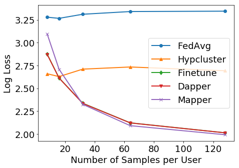
Figure 2: Test loss of algorithms as a function of number of samples per user for the synthetic dataset.

The details of the distributions are in Appendix F.1. We evaluate the algorithms as we vary the number of samples per user. The results are in Figure 2. HypCluster performs the best when the number of samples per user $m_{k}$ is very small. If $m_{k}$ is large, Mapper performs the best followed closely by Finetune and Dapper. However, the difference between Finetune and Dapper is statistically insignificant. In order to understand the effect of clustering, we evaluate various clustering algorithms as a function of $q$ when $m_{k}=100$, and the results are in Table 1. Since the clients are naturally divided into four clusters, as we increase $q$, the test loss steadily decreases till the number of clusters reaches $4$ and then remains constant.

7.2 EMNIST dataset

We evaluate the proposed algorithms on the federated EMNIST-62 dataset (Caldas et al., 2018) provided by TensorFlow Federated (TFF). The dataset consists of 3400 users’ examples that are each one of 62 classes. We select 2500 users to train the global models (referred to as seen) and leave the remaining 900 as unseen clients reserved for evaluation only. We shuffle the clients first before splitting as the original client ordering results in disjoint model performance. The reported metrics are uniformly averaged across clients similar to previous works (Jiang et al., 2019). For model architecture, we use a two-layer convolutional neural net. We refer to Appendix F.2 for more details on the architecture and training procedure.

The test results for seen and unseen clients are in Table 2 and Table 3, respectively. We trained models with FedAvg, Agnostic (Mohri et al., 2019), and HypCluster and combined them with Finetune, Dapper, and Mapper. We observe that HypCluster with two clusters performs significantly better compared to FedAvg and Agnostic models and improves accuracy by at least $4.3\%$. Thus clustering is significantly better than training a single global model.

The remaining algorithms Dapper and Mapper improve the accuracy by another $~{}1\%$ compared to HypCluster, but the EMNIST dataset is small and standard deviation in our experiments was in the order of $0.1\%$ and hence their improvement over Finetune is not statistically significant. However, these algorithms have provable generalization guarantees and thus would be more risk averse.

8 Conclusion

We presented a systematic learning-theoretic study of personalization in learning and proposed and analyzed three algorithms: user clustering, data interpolation, and model interpolation. For all three approaches, we provided learning theoretic guarantees and efficient algorithms. Finally, we empirically demonstrated the usefulness of the proposed approaches on synthetic and EMNIST datasets.

9 Acknowledgements

Authors thank Rajiv Mathews, Brendan Mcmahan, Ke Wu, and Shanshan Wu for helpful comments and discussions.

Appendix A Related works

A.1 Federated learning

FL was introduced by McMahan et al. (2017) as an efficient method for training models in a distributed way. They proposed a new communication-efficient optimization algorithm called FedAvg. They also showed that the training procedure provides additional privacy benefits. The introduction of FL has given rise to several interesting research problems, including the design of more efficient communication strategies (Konečnỳ et al., 2016b, a; Suresh et al., 2017; Stich, 2018; Karimireddy et al., 2019), the study of lower bounds for parallel stochastic optimization with a dependency graph (Woodworth et al., 2018), devising efficient distributed optimization methods benefiting from differential privacy guarantees (Agarwal et al., 2018), stochastic optimization solutions for the agnostic formulation (Mohri et al., 2019), and incorporating cryptographic techniques (Bonawitz et al., 2017), meta-learning (Chen et al., 2018), see (Li et al., 2019; Kairouz et al., 2019) for an in-depth survey of recent work in FL.

Federated learning often results in improved performance, as reported in several learning problems, including next word prediction (Hard et al., 2018; Yang et al., 2018), vocabulary estimation (Chen et al., 2019a), emoji prediction (Ramaswamy et al., 2019), decoder models (Chen et al., 2019b), low latency vehicle-to-vehicle communication (Samarakoon et al., 2018), and predictive models in health (Brisimi et al., 2018).

A.2 Personalization in federated learning

There are several recent works that focus on multi-task and meta-learning in the context of federated learning. Smith et al. (2017) studied the problem of federated multi-task learning and proposed MOCHA, an algorithm that jointly learns parameters and a similarity matrix between user tasks. MOCHA tackles various aspects of distributed multitask learning including communication constraints, stragglers, and fault tolerance. They focus on the convex setting and their application to non-convex deep learning models where strong duality is no longer guaranteed is unclear.

Jiang et al. (2019) drew interesting connections between FedAvg and first-order model agnostic meta-learning (MAML) (Finn et al., 2017) and showed that FedAvg is in fact already a meta-learning algorithm. Fallah et al. (2020) also proposed to use the MAML objective in a global model training to obtain a better personalizable global model. Khodak et al. (2019) proposed ARUBA that improves upon gradient-based meta-learning approaches. A variational approach for multi-task learning was proposed by Corinzia and Buhmann (2019). Recently, Hanzely and Richtárik (2020) proposed to learn a model per user by adding an $\ell_{2}$ penalty on model parameters to ensure they are similar.

Another line of work uses a set of local parameters, which are trained per-client, and a set of global parameters, which are trained using FL. For example, Bui et al. (2019) proposed to use user-representations by having a set of client-specific local parameters, which are trained per-client and a set of global parameters, which are trained using FL. Arivazhagan et al. (2019); Liang et al. (2020) proposed to store some layers of the model locally, while training the rest of the model with federated learning.

Peterson et al. (2019) proposed to use techniques from a mixture of experts literature and their approach is similar to our approach of model interpolation, but they learn an interpolation weight based on features. Furthermore, there are no theoretical guarantees for their approach. A theoretical analysis of interpolation models without variable mixing weights was recently presented in Agarwal et al. (2020). Concurrent to this work, Deng et al. (2020) proposed to use an interpolation of a local and global model. Their approach is similar to model interpolation in our paper.

Wang et al. (2019) showed that federated models can be fine-tuned based on local data. They proposed methods to find the best hyper-parameters for fine-tuning and showed that it improves the next word prediction of language models in virtual keyboard applications. Yu et al. (2020) proposed several variants of the fine-tuning approach, including training only a few layers of the networks, adding a local penalty term in the form of model distillation, or elastic weight averaging to the fine-tuning objective to improve local adaptation.

Zhao et al. (2018b) showed that one can improve the accuracy of FedAvg, by sharing a small amount of public data to reduce the non-i.i.d. nature of the client data. Sattler et al. (2019) proposed to use cosine-similarity between gradient updates for clustering in federated learning. However, their approach requires all clients to participate in each round and hence is computationally infeasible. Personalization in other settings such as peer-to-peer networks have been studied by Zantedeschi et al. (2019). We refer the readers to (Kulkarni et al., 2020) for a survey of algorithms for personalization in FL.

Appendix B Global models

B.1 Example for the suboptimality of global models

We provide the following simple example, which shows that global models can be a constant worse compared to the local model.

Example B.1.

Let $\mathcal{X}=\mathbb{R}$ and $\mathcal{Y}=\{0,1\}$. Suppose there are two clients with distributions ${\mathscr{D}}_{1}$ and ${\mathscr{D}}_{2}$ defined as follows. $\forall x,{\mathscr{D}}_{1}(x)={\mathscr{D}}_{2}(x)$ and ${\mathscr{D}}_{1}(1|x)=1$ if $x>0$ and zero otherwise. Similarly, ${\mathscr{D}}_{2}(1|x)=1$ only if $x<0$ and zero otherwise. Let $\mathcal{H}$ be the class of threshold classifiers indexed by a threshold $t\in\mathbb{R}$ and sign $s\in\{-1,1\}$ such that $h_{t,s}\in\mathcal{H}$ is given by $h_{t,s}(x)=1_{(x-t)s>0}$. Further, suppose we are interested in zero-one loss and the number of samples from both domains is very large and equal.

The optimal classifier for ${\mathscr{D}}_{1}$ is $h_{0,1}$ and the optimal classifier for ${\mathscr{D}}_{2}$ is $h_{0,-1}$, and they achieve zero error in their respective clients. Since the number of samples is the same from both clients, ${\mathscr{U}}$ is the uniform mixture of the two domains, ${\mathscr{U}}=0.5{\mathscr{D}}_{1}+0.5{\mathscr{D}}_{2}$ . Note that for all $h\in{\mathscr{H}}$, ${\mathscr{L}}_{{\mathscr{U}}}(h)=0.5$ and hence the global objective cannot differentiate between any of the hypotheses in $\mathcal{H}$. Thus, with high probability, any globally trained model incurs a constant loss on both clients.

B.2 Agnostic global model

Instead of assigning weights proportional to the number of samples as in the uniform global model, we can weight them according to any $\lambda\in\Delta^{p}$. For example, instead of uniform sample weights, we can weight clients uniformly corresponding to $\lambda_{k}=\frac{1}{p}$, for all $k$. Let $\bar{\mathscr{D}}_{\lambda}$ denote the $\lambda$-weighted empirical distribution and let $h_{\bar{\mathscr{D}}_{\lambda}}$ be the minimizer of loss over $\bar{\mathscr{D}}_{\lambda}$. Instead of the uniform global model described in the previous section, we can use the agnostic loss, where we minimize the maximum loss over a set of distributions. Let $\Lambda\subseteq\Delta^{p}$. Agnostic loss is given by

$$\max_{\lambda\in\Lambda}{\mathscr{L}}_{\bar{{\mathscr{D}}}_{\lambda}}(h).$$

Let $h_{\bar{{\mathscr{D}}}_{\Lambda}}$ be the minimizer. Let ${\mathfrak{s}}(\Lambda,{\mathbf{m}})=\max_{\lambda\in\Lambda}{\mathfrak{s}}(\lambda,{\mathbf{m}})$. Let $\Lambda_{\epsilon}$ be an $\epsilon$-cover of $\Delta^{p}$. Let ${\mathbf{m}}$ denote the empirical distribution of samples $(m_{1}/m,m_{2}/m,\ldots,m_{p}/m)$. The skewness between the distributions $\lambda$ and ${\mathbf{m}}$ is defined as ${\mathfrak{s}}(\lambda,{\mathbf{m}})=\sum^{p}_{k=1}\frac{\lambda^{2}_{k}}{{\mathbf{m}}_{k}},$ where ${\mathbf{m}}_{k}=m_{k}/m$. With these definitions, the generalization guarantee of (Mohri et al., 2019, Theorem 2) for client one can be expressed as follows:

$${\mathscr{L}}_{{\mathscr{D}}_{1}}(h_{\widehat{{\mathscr{D}}}_{\Lambda_{\epsilon}}})\leq{\mathscr{L}}_{{\mathscr{D}}_{1}}(h_{{\mathscr{D}}_{1}})+\tilde{\mathcal{O}}\left(\sqrt{{\mathfrak{s}}(\Lambda_{\epsilon}||{\mathbf{m}})}\cdot\frac{\sqrt{d+\log\frac{|\Lambda_{\epsilon}|}{\delta}}}{\sqrt{m}}+\epsilon\right)+\text{disc}_{\mathcal{H}}({\mathscr{D}}_{1},{\mathscr{D}}_{\lambda*}),$$

where $\lambda^{*}=\operatorname*{argmax}_{\lambda}{\mathscr{L}}_{\bar{{\mathscr{D}}}_{\lambda}}(h_{\widehat{{\mathscr{D}}}_{\Lambda_{\epsilon}}})$ is the mixture weight where the trained model $h_{\widehat{{\mathscr{D}}}_{\Lambda_{\epsilon}}}$ has the highest loss. Hence, this approach would personalize well for hard distributions and can be considered as a step towards ensuring that models work for all distributions. In this work, we show that training a different model for each client would significantly improve the model performance.

Appendix C Supplementary material for clustering

C.1 Baselines

If we have meta-features about the data samples and clients, such as location or type of device, we can use them to find clusters. This can be achieved by algorithms such as $k$-means or variants. This approach depends on the knowledge of the meta-features and their relationship to the set of hypotheses under consideration. While it may be reasonable in many circumstances, it may not be always feasible. If there are no meta-features, a natural approach is to cluster using a Bregman divergence defined over the distributions ${\mathscr{D}}_{k}$ (Banerjee et al., 2005). However, it is likely that we would overfit as the generalization of the density estimation depends on the covering number of the class of distributions ${\mathscr{D}}_{1},{\mathscr{D}}_{2},\ldots,{\mathscr{D}}_{p}$, which in general can be much larger than that of the class of hypotheses $\mathcal{H}$. To overcome this, we propose an approach based on hypotheses under consideration which we discuss next.

C.2 Generalization of clustering algorithms

Recall that we solve for

$$\min_{h_{1},\ldots,h_{q}}\sum^{p}_{k=1}\frac{m_{k}}{m}\cdot\min_{i\in[q]}{\mathscr{L}}_{\widehat{{\mathscr{D}}}_{k}}(h_{i}).$$ (7)

Lemma C.1.

Let $h^{*}_{1},h^{*}_{2},\ldots,h^{*}_{q}$ be the $q$ models obtained by solving (3) and $\widehat{h}^{*}_{1},\widehat{h}^{*}_{2},\ldots,\widehat{h}^{*}_{q}$ be the $q$ models obtained by solving (7). Then,

$$\sum^{p}_{k=1}\frac{m_{k}}{m}\cdot\left(\min_{i\in[q]}{\mathscr{L}}_{{\mathscr{D}}_{k}}(\widehat{h}^{*}_{i})-\min_{i\in[q]}{\mathscr{L}}_{{\mathscr{D}}_{k}}(h^{*}_{i})\right)\leq 2\max_{h_{1},\ldots,h_{q}}\left\lvert\sum^{p}_{k=1}\frac{m_{k}}{m}\cdot\left(\min_{i\in[q]}{\mathscr{L}}_{{\mathscr{D}}_{k}}(h_{i})-\min_{i\in[q]}{\mathscr{L}}_{\widehat{{\mathscr{D}}}_{k}}(h_{i})\right)\right\rvert.$$ (8)

Proof C.2.

$$\sum^{p}_{k=1}\frac{m_{k}}{m}\cdot\min_{i\in[q]}{\mathscr{L}}_{{\mathscr{D}}_{k}}(\widehat{h}^{*}_{i})-\sum^{p}_{k=1}\frac{m_{k}}{m}\cdot\min_{i\in[q]}{\mathscr{L}}_{{\mathscr{D}}_{k}}(h^{*}_{i})$$

$$=\sum^{p}_{k=1}\frac{m_{k}}{m}\cdot\min_{i\in[q]}{\mathscr{L}}_{{\mathscr{D}}_{k}}(\widehat{h}^{*}_{i})+\sum^{p}_{k=1}\frac{m_{k}}{m}\cdot\min_{i\in[q]}{\mathscr{L}}_{\widehat{{\mathscr{D}}}_{k}}(\widehat{h}^{*}_{i})-\sum^{p}_{k=1}\frac{m_{k}}{m}\cdot\min_{i\in[q]}{\mathscr{L}}_{\widehat{{\mathscr{D}}}_{k}}(\widehat{h}^{*}_{i})$$

$$+\sum^{p}_{k=1}\frac{m_{k}}{m}\cdot\min_{i\in[q]}{\mathscr{L}}_{\widehat{{\mathscr{D}}}_{k}}(h^{*}_{i})-\sum^{p}_{k=1}\frac{m_{k}}{m}\cdot\min_{i\in[q]}{\mathscr{L}}_{{\mathscr{D}}_{k}}(h^{*}_{i})-\sum^{p}_{k=1}\frac{m_{k}}{m}\cdot\min_{i\in[q]}{\mathscr{L}}_{\widehat{{\mathscr{D}}}_{k}}(h^{*}_{i})$$

$$\leq 2\max_{h_{1},\ldots,h_{q}}\left\lvert\sum^{p}_{k=1}\frac{m_{k}}{m}\cdot\min_{i\in[q]}{\mathscr{L}}_{{\mathscr{D}}_{k}}(h_{i})-\sum^{p}_{k=1}\frac{m_{k}}{m}\cdot\min_{i\in[q]}{\mathscr{L}}_{\widehat{{\mathscr{D}}}_{k}}(h_{i})\right\rvert,$$

where the inequality follows by observing that $\sum^{p}_{k=1}\frac{m_{k}}{m}\cdot\min_{i\in[q]}{\mathscr{L}}_{\widehat{{\mathscr{D}}}_{k}}(\widehat{h}^{*}_{i})\leq\sum^{p}_{k=1}\frac{m_{k}}{m}\cdot\min_{i\in[q]}{\mathscr{L}}_{\widehat{{\mathscr{D}}}_{k}}(h^{*}_{i})$, by the definition of $\widehat{h}^{*}_{i}$.

C.3 Proof of Theorem 4.1

For any set of real numbers $a_{1},a_{2},\ldots,a_{q}$ and $b_{1},b_{2},\ldots,b_{q}$, observe that

$$\min_{i}a_{i}-\min_{i}b_{i} =\min_{i}b_{i}+(a_{i}-b_{i})-\min_{i}b_{i}\leq\min_{i}b_{i}+\max_{i}(a_{i}-b_{i})-\min b_{i}=\max_{i}(a_{i}-b_{i}).$$

We first prove the theorem for one side. Let $f\colon[p]\to[q]$ be a mapping from clients to clusters. Applying the above result yields,

$$\max_{h_{1},\ldots,h_{q}}\left(\sum^{p}_{k=1}m_{k}\cdot\min_{i\in[q]}{\mathscr{L}}_{{\mathscr{D}}_{k}}(h_{k})-\sum^{p}_{k=1}m_{k}\cdot\min_{i\in[q]}{\mathscr{L}}_{\widehat{{\mathscr{D}}}_{k}}(h_{k})\right)$$

$$\leq\max_{h_{1},\ldots,h_{q}}\left(\sum^{p}_{k=1}m_{k}\cdot\max_{k\in[p]}({\mathscr{L}}_{{\mathscr{D}}_{k}}(h_{k})-{\mathscr{L}}_{\widehat{{\mathscr{D}}}_{k}}(h_{k}))\right)$$

$$=\max_{h_{1},\ldots,h_{q}}\left(\sum^{p}_{k=1}m_{k}\cdot\max_{f(k)}({\mathscr{L}}_{{\mathscr{D}}_{k}}(h_{f(k)})-{\mathscr{L}}_{\widehat{{\mathscr{D}}}_{k}}(h_{f(k)}))\right)$$

$$=\max_{h_{1},\ldots,h_{q}}\max_{f}\left(\sum^{p}_{k=1}m_{k}\cdot({\mathscr{L}}_{{\mathscr{D}}_{k}}(h_{f(k)})-{\mathscr{L}}_{\widehat{{\mathscr{D}}}_{k}}(h_{f(k)}))\right)$$

$$=\max_{f}\max_{h_{1},\ldots,h_{q}}\left(\sum^{p}_{k=1}m_{k}\cdot({\mathscr{L}}_{{\mathscr{D}}_{k}}(h_{f(k)})-{\mathscr{L}}_{\widehat{{\mathscr{D}}}_{k}}(h_{f(k)}))\right).$$

Since changing one sample changes the above function by at most $1$, for a given $f$, by the McDiarmid’s inequality, with probability at least $1-\delta$, the following holds:

$$\max_{h_{1},\ldots,h_{q}}\left(\sum^{p}_{k=1}m_{k}\cdot({\mathscr{L}}_{{\mathscr{D}}_{k}}(h_{f(k)})-{\mathscr{L}}_{\widehat{{\mathscr{D}}}_{k}}(h_{f(k)}))\right)$$

$$\leq\operatorname*{\mathbb{E}}\left[\max_{h_{1},\ldots,h_{q}}\left(\sum^{p}_{k=1}m_{k}\cdot({\mathscr{L}}_{{\mathscr{D}}_{k}}(h_{f(k)})-{\mathscr{L}}_{\widehat{{\mathscr{D}}}_{k}}(h_{f(k)}))\right)\right]+2\sqrt{m\log\frac{1}{\delta}}.$$

The number of possible functions $f$ is $q^{p}$. Hence, by the union bound, for all $f$, with probability at least $1-\delta$, the following holds:

$$\max_{h_{1},\ldots,h_{q}}\left(\sum^{p}_{k=1}m_{k}\cdot({\mathscr{L}}_{{\mathscr{D}}_{k}}(h_{f(k)})-{\mathscr{L}}_{\widehat{{\mathscr{D}}}_{k}}(h_{f(k)}))\right)$$

$$\leq\operatorname*{\mathbb{E}}\left[\max_{h_{1},\ldots,h_{q}}\left(\sum^{p}_{k=1}m_{k}\cdot({\mathscr{L}}_{{\mathscr{D}}_{k}}(h_{f(k)})-{\mathscr{L}}_{\widehat{{\mathscr{D}}}_{k}}(h_{f(k)}))\right)\right]+2\sqrt{mp\log\frac{q}{\delta}}.$$

For a given clustering $f$, by the sub-additivity of $\max$,

$$\max_{h_{1},\ldots,h_{q}}\left(\sum^{p}_{k=1}m_{k}\cdot({\mathscr{L}}_{{\mathscr{D}}_{k}}(h_{f(k)})-{\mathscr{L}}_{\widehat{{\mathscr{D}}}_{k}}(h_{f(k)}))\right)$$

$$=\max_{h_{1},\ldots,h_{q}}\left(\sum^{p}_{k=1}\sum_{k:f(k)=i}m_{k}\cdot({\mathscr{L}}_{{\mathscr{D}}_{k}}(h_{f(k)})-{\mathscr{L}}_{\widehat{{\mathscr{D}}}_{k}}(h_{f(k)}))\right)$$

$$\leq\sum^{q}_{i=1}\max_{h_{1},\ldots,h_{q}}\left(\sum_{k:f(k)=i}m_{k}\cdot({\mathscr{L}}_{{\mathscr{D}}_{k}}(h_{f(k)})-{\mathscr{L}}_{\widehat{{\mathscr{D}}}_{k}}(h_{f(k)}))\right)$$

$$=\sum^{q}_{i=1}\max_{h_{1},\ldots,h_{q}}\left(\sum_{k:f(k)=i}m_{k}\cdot({\mathscr{L}}_{{\mathscr{D}}_{k}}(h_{i})-{\mathscr{L}}_{\widehat{{\mathscr{D}}}_{k}}(h_{i}))\right)$$

$$=\sum^{q}_{i=1}\max_{h_{i}}\left(\sum_{k:f(k)=i}m_{k}\cdot({\mathscr{L}}_{{\mathscr{D}}_{k}}(h_{i})-{\mathscr{L}}_{\widehat{{\mathscr{D}}}_{k}}(h_{i}))\right)$$

$$=\sum^{q}_{i=1}\max_{h_{i}}\left(m_{C_{i}}\cdot({\mathscr{L}}_{{\mathscr{C}}_{i}}(h_{i})-{\mathscr{L}}_{\widehat{{\mathscr{C}}}_{i}}(h_{i}))\right),$$

where $C_{i}$ is the cluster of clients such that $f(k)=i$ and $m_{C_{i}}$ is the number of samples in that cluster, and ${\mathscr{C}}_{i}$ is its distribution. Thus,

$$\operatorname*{\mathbb{E}}\left[\max_{h_{1},\ldots,h_{q}}\left(\sum^{p}_{k=1}m_{k}\cdot({\mathscr{L}}_{{\mathscr{D}}_{k}}(h_{f(k)})-{\mathscr{L}}_{\widehat{{\mathscr{D}}}_{k}}(h_{f(k)}))\right)\right] \leq\operatorname*{\mathbb{E}}\left[\sum^{q}_{i=1}\max_{h_{i}}\left(m_{C_{i}}\cdot({\mathscr{L}}_{{\mathscr{C}}_{i}}(h_{i})-{\mathscr{L}}_{\widehat{{\mathscr{C}}}_{i}}(h_{i}))\right)\right]$$

$$\leq\sum^{q}_{i=1}{\mathfrak{R}}_{{\mathscr{C}}_{i},m_{C_{i}}}({\mathscr{H}})m_{C_{i}},$$

where the last inequality follows from standard learning-theoretic guarantees and the definition of Rademacher complexity (Mohri et al., 2018). The proof follows by combining the above equations, normalizing by $m$, and the union bound.

C.4 Proof of Corollary 4.2

We show that for any clustering,

$$\sum^{q}_{i=1}\frac{m_{C_{i}}}{m}{\mathfrak{R}}_{{\mathscr{C}}_{i},m_{C_{i}}}({\mathscr{H}})\leq\sqrt{\frac{dp}{m}\log\frac{em}{d}}.$$

The proof then follows from Theorem 4.1. To prove the above observation, observe that

$$\sum^{q}_{i=1}\frac{m_{C_{i}}}{m}{\mathfrak{R}}_{{\mathscr{C}}_{i},m_{C_{i}}}({\mathscr{H}}) \leq\sum^{q}_{i=1}\frac{m_{C_{i}}}{m}\sqrt{\frac{dp}{m_{C_{i}}}\log\frac{em_{C_{i}}}{d}}\leq\sum^{q}_{i=1}\frac{m_{C_{i}}}{m}\sqrt{\frac{dp}{m_{C_{i}}}\log\frac{em}{d}}$$

$$\leq\sum^{q}_{i=1}\frac{1}{m}\sum^{q}_{i=1}\sqrt{{dp}{m_{C_{i}}}\log\frac{em}{d}}\leq\sqrt{\frac{dq}{m}\log\frac{em}{d}},$$

where the last inequality follows from Jensen’s inequality.

Appendix D Supplementary material for data interpolation

D.1 Proof of Theorem 5.2

Let $g(h)=\lambda{\mathscr{L}}_{\widehat{{\mathscr{D}}}_{k}}(h)+(1-\lambda){\mathscr{L}}_{\widehat{{\mathscr{C}}}}(h)$. Suppose we are interested in running $T$ steps of SGD on $g$, where at each step we independently sample $\widehat{{\mathscr{D}}}_{k}$ with probability $\lambda$ and $\widehat{{\mathscr{C}}}$ with probability $1-\lambda$ and choose a random sample from the selected empirical distribution to compute the gradient. This can be simulated by first sampling $T$ elements from $\widehat{{\mathscr{C}}}$, denoted by $\widehat{{\mathscr{C}}}^{\prime}$ and using $\widehat{{\mathscr{C}}}^{\prime}$ instead of $\widehat{{\mathscr{C}}}$ during optimization. Hence to prove the theorem, suffices to show that $T=rm_{k}$ steps of SGD on $g$ using the above mentioned sampling procedure yields the desired bound.

We now ask how large should $T$ be to obtain error of $\epsilon_{\lambda}$. By standard stochastic gradient descent guarantees, the output $h_{A}$ satisfies

$$\operatorname*{\mathbb{E}}[g(h_{A})]\leq\operatorname*{\mathbb{E}}[g(h_{\widehat{\lambda}})]+\frac{\|h_{c}-h_{\widehat{\lambda}})\|^{2}}{2\eta}+\frac{\eta G^{2}T}{2}.$$

Since the loss is strongly convex and $h_{c}$ is optimal for ${\mathscr{L}}_{\widehat{{\mathscr{C}}}}(h_{c})$,

$${\mathscr{L}}_{\widehat{{\mathscr{C}}}}(h_{\widehat{\lambda}})-{\mathscr{L}}_{\widehat{{\mathscr{C}}}}(h_{c})\geq\frac{\mu}{2}\|h_{c}-h_{\widehat{\lambda}})\|^{2}.$$

Furthermore, since $h_{\widehat{\lambda}}$ is optimal for a $\lambda$-mixture,

$$\lambda{\mathscr{L}}_{\widehat{{\mathscr{D}}}_{k}}(h_{\widehat{\lambda}})+(1-\lambda){\mathscr{L}}_{\widehat{{\mathscr{C}}}}(h_{\widehat{\lambda}})\leq\lambda{\mathscr{L}}_{\widehat{{\mathscr{D}}}_{k}}(h_{c})+(1-\lambda){\mathscr{L}}_{\widehat{{\mathscr{C}}}}(h_{c}).$$

Hence,

$$\frac{\mu}{2}\|h_{c}-h_{\widehat{\lambda}})\|^{2} \leq{\mathscr{L}}_{\widehat{{\mathscr{C}}}}(h_{\widehat{\lambda}})-{\mathscr{L}}_{\widehat{{\mathscr{C}}}}(h_{c})$$

$$\leq\frac{\lambda}{1-\lambda}({\mathscr{L}}_{\widehat{{\mathscr{D}}}_{k}}(h_{c})-{\mathscr{L}}_{\widehat{{\mathscr{D}}}_{k}}(h_{\widehat{\lambda}}))$$

$$\leq\frac{G\lambda}{1-\lambda}\|h_{c}-h_{\widehat{\lambda}})\|.$$

Therefore,

$$\|h_{c}-h_{\widehat{\lambda}})\|\leq\min\left(\frac{2G\lambda}{\mu(1-\lambda)},R\right)$$

Combining the above equations, we get

$$\operatorname*{\mathbb{E}}[g(h_{A})]\leq\operatorname*{\mathbb{E}}[g(h_{\widehat{\lambda}})]+\frac{1}{2\eta}\min\left(\frac{2G\lambda}{\mu(1-\lambda)},R\right)^{2}+\frac{\eta G^{2}T}{2}.$$

Substituting the learning rate and setting $T=rm_{k}$ yields

$$\operatorname*{\mathbb{E}}[g(h_{A})]\leq\operatorname*{\mathbb{E}}[g(h_{\widehat{\lambda}})]+\frac{G}{\sqrt{rm_{k}}}\min\left(\frac{2G\lambda}{\mu(1-\lambda)},R\right).$$

Hence if $r\geq G^{2}\max_{\lambda}\min\left(\frac{2G}{\mu(1-\lambda)},\frac{R}{\lambda}\right)^{2}$, the above bound is at most $\sqrt{\frac{\lambda^{2}}{m_{k}}}\leq\epsilon_{\lambda}$. Note that for any $\lambda$,

$$\min\left(\frac{2G}{\mu(1-\lambda)},\frac{R}{\lambda}\right)\leq\frac{2G}{\mu(1-\lambda)}1_{\lambda<1/2}+\frac{R}{\lambda}1_{\lambda\geq 1/2}\leq\frac{4G}{\mu}+2R,$$

hence the theorem.

D.2 Dapper pseudo-code

We provide pseudo-code for the Dapper algorithm in Figure 3.

Algorithm Dapper($h_{c}$) For each client $k$ do the following: 1. Randomly sample $r\cdot m_{k}$ data points from $\widehat{{\mathscr{C}}}$. Let this dataset be $\widehat{{\mathscr{C}}^{\prime}}$. 2. Let $\Lambda$ be a cover of $[0,1]$. For each $\lambda\in\Lambda$, the client starts with $h_{c}$ and minimizes $$\lambda{\mathscr{L}}_{\widehat{{\mathscr{D}}}_{k}}(h)+(1-\lambda){\mathscr{L}}_{\widehat{{\mathscr{C}}^{\prime}}}(h)$$ (9) using stochastic gradient descent for $r\cdot m_{k}$ steps, where at each step, it selects $\widehat{{\mathscr{D}}}_{k}$ with probability $\lambda$ and $\widehat{{\mathscr{C}}}^{\prime}$ with probability $1-\lambda$ and samples an element from the corresponding dataset to compute the stochastic gradient. Let $h_{\lambda}$ be the resulting model and ${\mathscr{H}}_{\Lambda}=\{h_{\lambda}:\lambda\in\Lambda\}$. 3. Output $$\operatorname*{argmin}_{h\in{\mathscr{H}}_{\Lambda}}{\mathscr{L}}_{\widehat{{\mathscr{D}}}_{k}}(h).$$

Figure 3: Pseudocode for the Dapper algorithm.

D.3 Practical considerations

While the above algorithm reduces the amount of data transfer and is computationally efficient, it may be vulnerable to privacy issues in applications such as FL. To overcome that, we propose several alternatives:

1. Sufficient statistics: in many scenarios, instead of the actual data, we only need some sufficient statistics. For example in regression with $\ell^{2}_{2}$ loss, we only need the covariance matrix of the dataset from $\widehat{{\mathscr{C}}}$.

2. Generative models: for problems such as density estimation and language modelling, we can use the centralized model to generate synthetic samples from $h_{c}$ and use that as an approximation to $\widehat{{\mathscr{C}}^{\prime}}$. For other applications, one can train a GAN and send the GAN to the clients and the clients can sample from the GAN to create the dataset $\widehat{{\mathscr{C}}^{\prime}}$ (Augenstein et al., 2019).

3. Proxy public data: if it is not feasible to send the actual user data, one could send proxy public data instead. While this may not be theoretically optimal, it will still avoid overfitting to the local data.

Appendix E Supplementary material for model interpolation

E.1 Proof of Theorem 6.1

Observe that

$$\sum^{p}_{k=1}\frac{m_{k}}{m}{\mathscr{L}}_{{{\mathscr{D}}_{k}}}((1-\widehat{\lambda}^{*}_{k})\widehat{h}^{*}_{c}+\lambda^{*}_{k}\widehat{h}^{*}_{l,k})-\sum^{p}_{k=1}\frac{m_{k}}{m}{\mathscr{L}}_{{{\mathscr{D}}_{k}}}((1-{\lambda^{*}_{k}}){h^{*}_{c}}+\lambda^{*}_{k}{h^{*}_{l,k}})$$

$$\leq 2\max_{h_{c},\bar{\lambda},\bar{h}_{l}}\left(\sum^{p}_{k=1}\frac{m_{k}}{m}\left({\mathscr{L}}_{{{\mathscr{D}}_{k}}}((1-{\lambda_{k}}){h_{c}}+\lambda_{k}{h_{l,k}})-{\mathscr{L}}_{\widehat{{\mathscr{D}}}_{k}}((1-{\lambda_{k}}){h_{c}}+\lambda_{k}{h_{l,k}})\right)\right).$$

Changing one sample changes the above function by at most $1/m$. Thus by McDiarmid’s inequality, with probability at least $1-\delta$,

$$\max_{h_{c},\bar{\lambda},\bar{h}_{l}}\left(\sum^{p}_{k=1}\frac{m_{k}}{m}\left({\mathscr{L}}_{{{\mathscr{D}}_{k}}}((1-{\lambda_{k}}){h_{c}}+\lambda_{k}{h_{l,k}})-{\mathscr{L}}_{\widehat{{\mathscr{D}}}_{k}}((1-{\lambda_{k}}){h_{c}}+\lambda_{k}{h_{l,k}})\right)\right)$$

$$\leq\operatorname*{\mathbb{E}}\left[\max_{h_{c},\bar{\lambda},\bar{h}_{l}}\left(\sum^{p}_{k=1}\frac{m_{k}}{m}\left({\mathscr{L}}_{{{\mathscr{D}}_{k}}}((1-{\lambda_{k}}){h_{c}}+\lambda_{k}{h_{l,k}})-{\mathscr{L}}_{\widehat{{\mathscr{D}}}_{k}}((1-{\lambda_{k}}){h_{c}}+\lambda_{k}{h_{l,k}})\right)\right)\right]+2\sqrt{\frac{\log\frac{1}{\delta}}{m}}.$$

Let $\bar{{\mathscr{H}}}_{l}$ be the Cartesian product of hypothesis classes where the $k^{\text{th}}$ hypothesis class is the hypothesis applied to $k^{\text{th}}$ client. Let ${\mathscr{H}}=\bar{\lambda}{\mathscr{H}}_{c}+(1-\bar{\lambda})\bar{{\mathscr{H}}}_{l}$. Hence, by Talagrand’s construction lemma and the properties of Rademacher complexity,

$$\operatorname*{\mathbb{E}}\left[\max_{h_{c},\bar{\lambda},\bar{h}_{l}}\left(\sum^{p}_{k=1}\frac{m_{k}}{m}\left({\mathscr{L}}_{{{\mathscr{D}}_{k}}}((1-{\lambda_{k}}){h_{c}}+\lambda_{k}{h_{l,k}})-{\mathscr{L}}_{\widehat{{\mathscr{D}}}_{k}}((1-{\lambda_{k}}){h_{c}}+\lambda_{k}{h_{l,k}})\right)\right)\right]$$

$$\leq{\mathfrak{R}}_{{\mathscr{U}}+\bar{{\mathscr{D}}},\bar{m}}(\ell({\mathscr{H}}))$$

$$\leq L{\mathfrak{R}}_{{\mathscr{U}}+\bar{{\mathscr{D}}},\bar{m}}({\mathscr{H}})$$

$$\leq L{\mathfrak{R}}_{{\mathscr{U}},m}({\mathscr{H}}_{c})+L\mathbb{R}_{{\mathscr{D}}_{k},m_{k}}(\bar{{\mathscr{H}}}_{l})$$

$$\leq L\left({\mathfrak{R}}_{{\mathscr{U}},m}({\mathscr{H}}_{c})+\sum^{p}_{k=1}\frac{m_{k}}{m}{\mathfrak{R}}_{{\mathscr{D}}_{k},m_{k}}({\mathscr{H}}_{l})\right),$$

where the last inequality follows from the sub-additivity of Rademacher complexity.

E.2 Mapper algorithms

We first show that this method of independently finding the local models is sub-optimal with an example.

Example E.1.

Consider the following discrete distribution estimation problem. Let $\mathcal{H}_{c}$ be the set of distributions over $d$ values and let $\mathcal{H}_{l}$ be the set of distributions with support size $1$. For even $k$, let ${\mathscr{D}}_{k}(1)={\mathscr{D}}_{\text{even}}(1)=1.0$ and for odd $k$, let ${\mathscr{D}}_{k}(y)={\mathscr{D}}_{\text{odd}}(y)=1/d$ for all $1\leq y\leq d$. Let the number of clients $p$ be very large and the number of samples per client a constant, say ten. Suppose we consider the log-loss.

The intuition behind this example is that since we have only one example per domain, we can only derive good estimates for the local model for even $k$ and we need to estimate the global model jointly from the odd clients. With this approach, the optimal solution is as follows. For even $k$, $h_{l,k}={\mathscr{D}}_{k}$ and $\lambda_{k}=1.0$. For odd $k$, $\lambda_{k}=0.0$ and the optimal $h_{c}$ is given by, $h_{c}={\mathscr{D}}_{\text{odd}}$. If we learn the models separately, observe that, for each client $\widehat{h}_{l,k}$ be the empirical estimate and $\widehat{h}_{c}$ would be $0.5\cdot{\mathscr{D}}_{\text{even}}+0.5\cdot{\mathscr{D}}_{\text{odd}}$. Thus, for any $\bar{\lambda}$, the algorithm would incur at least a constant loss more than optimal for any $\lambda_{k}$ for odd clients.

Algorithm Mapper Randomly initialize $h^{0}_{c}$ and for $t=1$ to $T$, randomly select a client $k$ and do the following. 1. Let $\Lambda$ be a cover of $[0,1]$. For each $\lambda\in\Lambda$, let $$h_{l,k}(\lambda)=\operatorname*{argmin}_{h_{l,k}}{\mathscr{L}}_{\widehat{{\mathscr{D}}}_{k}}(\lambda h_{l,k}+(1-\lambda)h^{t-1}_{c}).$$ (10) 2. Find the best local model: $$\lambda^{*}=\operatorname*{argmin}_{\lambda\in\Lambda}{\mathscr{L}}_{\widehat{{\mathscr{D}}}_{k}}(\lambda h_{l,k}(\lambda)+(1-\lambda)h^{t-1}_{c}).$$ (11) 3. Minimize the global model. $$h^{t}_{c}=h^{t-1}_{c}-\eta\nabla{\mathscr{L}}_{\widehat{{\mathscr{D}}}_{k}}(\lambda^{*}h_{l,k}(\lambda^{*})+(1-\lambda^{*})h^{t-1}_{c}).$$ (12) Let $h^{T}_{c}$ be the final global model. For each client $k$ rerun $1(a)$ and $1(b)$ to obtain the local model $h_{l,k}$ and the interpolation weight $\lambda_{k}$.

Figure 4: Pseudocode for the Mapper algorithm.

Since training models independently is sub-optimal in certain cases, we propose a joint-optimization algorithm. First observe that the optimization can be rewritten as

$$\min_{h_{c}}\sum^{p}_{k=1}\frac{m_{k}}{m}\min_{\bar{h}_{l}\bar{\lambda}}{\mathscr{L}}_{\widehat{{\mathscr{D}}}_{k}}((1-\lambda_{k})h_{c}+\lambda_{k}h_{l,k}).$$

Notice that for a fixed $\lambda$ the function is convex in both $h^{\ell}$ and $h_{c}$. But with the minimization over $\lambda$, the function is no longer convex. We propose algorithm Mapper for minimizing the interpolation models. At each round, the algorithm randomly selects a client. It then finds the best local model and interpolation weight for that client using the current value of the global model. It then updates the global model using the local model and the interpolation weight found in the previous step.

Appendix F Supplementary material for experiments

F.1 Synthetic dataset

Let $U$ be a uniform distribution over ${\mathscr{Y}}$. Let $P_{k}$ be a point mass distribution with $P_{k}(k)=1.0$ and for all $y\neq k$, $P_{k}(y)=0$. For a client $k$, let ${\mathscr{D}}_{k}$ be a mixture given by

$${\mathscr{D}}_{k}=0.5\cdot P_{k\%4}+0.25\cdot U+0.25\cdot P_{k\%(d-4)},$$

where $a\%b$, is $a$ modulo $b$. Roughly, $U$ is the uniform component and is same for all the clients, $P_{k\%4}$ is the cluster component and same for clients with same clusters, and $P_{k\%(d-4)}$ is the individual component per client.

F.2 EMNIST dataset

Table 4: EMNIST convolutional model.

Layer	Output Shape	# Parameters	Activation	Hyperparameters
Conv2d	(26, 26, 32)	320	ReLU	out_chan=32;filter_shape=(3, 3)
Conv2d	(24, 24, 64)	18496	ReLU	out_chan=64;filter_shape=(3, 3)
MaxPool2d	(12, 12, 64)	0		window_shape=(2, 2);strides=(2, 2)
Dropout	(12, 12, 64)	0		keep_rate=0.75
Flatten	9216	0
Dense	128	1179776	ReLU
Dropout	128	0		keep_rate=0.5
Dense	62	7998	LogSoftmax

For the EMNIST experiments, we follow previous work for model architecture (Jiang et al., 2019). The full model architecture layer by layer is provided in Table 4. We train the model for 1000 communication rounds with 20 clients per round and use server side momentum, though one can use different optimizers (Jiang et al., 2019). Evaluating the combined effect of our approach and adaptive optimizers remains an interesting open direction. Additionally, we apply logit smoothing with weight = 0.9 to the loss function to mitigate against exploding gradients experienced often in training federated models.

For all algorithms, the following hyperparameters are the same: client batch size=20, num clients per round=20, num rounds=1000, server learning rate=1.0, server momentum=0.9. For the remaining hyperparameters, we perform a sweep over parameters and use the eval dataset to choose the best. The best hyperparameters after sweeping are as follows.

• FedAvg: client num epochs=1, client step size=0.05.

• Agnostic: client num epochs=1, client step size=0.05, domain learning rate=0.05. NIST documentation shows that the EMNIST dataset comes from two writer sources: Census and High School (Grother, 1995). We use these two distinct sources as domains.

• HypCluster: client num epochs=1, client step size=0.03, num clusters=2. We determined that 2 was the optimal number of clusters since for larger numbers of clusters, all clients essentially mapped to just 2 of them.

• Finetune: client num epochs=5, client step size=0.01. We use the best baseline model as the pre-trained starting global model and finetune for each client.

• Dapper: client num epochs=1, client step size=0.04. Similar to Finetune, we use the best baseline model as the pre-trained starting global model. For each client, we finetune the global model using a mixture of global and client data. Given $m_{k}$ client examples, we sample $5\cdot m_{k}$ global examples.

• Mapper: client num epochs=1, client step size=0.03 . We use the same global hyperparameters as the starting global model with the above local hyperparameters. As stated previously, we use the same architecture for both local and global models and at each optimization step, we initialize the local model using the global parameters.

Over the course of running experiments, we observed a peculiar behavior regarding the original client ordering provided in the EMNIST dataset. If the seen and unseen split is performed on the original ordering of clients, the model performance between seen and unseen clients is very different. In particular, unseen is almost $10\%$ absolute worse than seen. Looking through the NIST documentation, we found that the data was sourced from two distinct sources: Census and High School (Grother, 1995). The original client ordering is derived from the data partition they are sourced from and High School clients were all in one split, resulting in the difference in model performance. Thus, we determined that shuffling the clients before splitting was better.

References

- Agarwal et al. (2020) Alekh Agarwal, John Langford, and Chen-Yu Wei. Federated residual learning. arXiv preprint arXiv:2003.12880, 2020.
- Agarwal et al. (2018) Naman Agarwal, Ananda Theertha Suresh, Felix X. Yu, Sanjiv Kumar, and Brendan McMahan. cpSGD: Communication-efficient and differentially-private distributed SGD. In Proceedings of NeurIPS, pages 7575–7586, 2018.
- Allenby et al. (2005) Greg M Allenby, Peter E Rossi, and Robert E McCulloch. Hierarchical bayes models: A practitioners guide. ssrn scholarly paper id 655541. Social Science Research Network, Rochester, NY, 2005.
- Arivazhagan et al. (2019) Manoj Ghuhan Arivazhagan, Vinay Aggarwal, Aaditya Kumar Singh, and Sunav Choudhary. Federated learning with personalization layers. arXiv preprint arXiv:1912.00818, 2019.
- Augenstein et al. (2019) Sean Augenstein, H. Brendan McMahan, Daniel Ramage, Swaroop Ramaswamy, Peter Kairouz, Mingqing Chen, Rajiv Mathews, et al. Generative models for effective ml on private, decentralized datasets. arXiv preprint arXiv:1911.06679, 2019.
- Banerjee et al. (2005) Arindam Banerjee, Srujana Merugu, Inderjit S Dhillon, and Joydeep Ghosh. Clustering with Bregman divergences. Journal of machine learning research, 6(Oct):1705–1749, 2005.
- Blitzer et al. (2008) John Blitzer, Koby Crammer, Alex Kulesza, Fernando Pereira, and Jennifer Wortman. Learning bounds for domain adaptation. In Advances in neural information processing systems, pages 129–136, 2008.
- Bonawitz et al. (2017) Keith Bonawitz, Vladimir Ivanov, Ben Kreuter, Antonio Marcedone, H. Brendan McMahan, Sarvar Patel, Daniel Ramage, Aaron Segal, and Karn Seth. Practical secure aggregation for privacy-preserving machine learning. In Proceedings of the 2017 ACM SIGSAC Conference on Computer and Communications Security, pages 1175–1191. ACM, 2017.
- Brisimi et al. (2018) Theodora S. Brisimi, Ruidi Chen, Theofanie Mela, Alex Olshevsky, Ioannis Ch. Paschalidis, and Wei Shi. Federated learning of predictive models from federated electronic health records. International journal of medical informatics, 112:59–67, 2018.
- Bui et al. (2019) Duc Bui, Kshitiz Malik, Jack Goetz, Honglei Liu, Seungwhan Moon, Anuj Kumar, and Kang G Shin. Federated user representation learning. arXiv preprint arXiv:1909.12535, 2019.
- Caldas et al. (2018) Sebastian Caldas, Peter Wu, Tian Li, Jakub Konečnỳ, H Brendan McMahan, Virginia Smith, and Ameet Talwalkar. Leaf: A benchmark for federated settings. arXiv preprint arXiv:1812.01097, 2018.
- Chen et al. (2018) Fei Chen, Mi Luo, Zhenhua Dong, Zhenguo Li, and Xiuqiang He. Federated meta-learning with fast convergence and efficient communication. arXiv preprint arXiv:1802.07876, 2018.
- Chen et al. (2019a) Mingqing Chen, Rajiv Mathews, Tom Ouyang, and Françoise Beaufays. Federated learning of out-of-vocabulary words. arXiv preprint arXiv:1903.10635, 2019a.
- Chen et al. (2019b) Mingqing Chen, Ananda Theertha Suresh, Rajiv Mathews, Adeline Wong, Françoise Beaufays, Cyril Allauzen, and Michael Riley. Federated learning of N-gram language models. In Proceedings of the 23rd Conference on Computational Natural Language Learning (CoNLL), 2019b.
- Corinzia and Buhmann (2019) Luca Corinzia and Joachim M Buhmann. Variational federated multi-task learning. arXiv preprint arXiv:1906.06268, 2019.
- Deng et al. (2020) Yuyang Deng, Mohammad Mahdi Kamani, and Mehrdad Mahdavi. Adaptive personalized federated learning. arXiv preprint arXiv:2003.13461, 2020.
- Fallah et al. (2020) Alireza Fallah, Aryan Mokhtari, and Asuman Ozdaglar. Personalized federated learning: A meta-learning approach. arXiv preprint arXiv:2002.07948, 2020.
- Finn et al. (2017) Chelsea Finn, Pieter Abbeel, and Sergey Levine. Model-agnostic meta-learning for fast adaptation of deep networks. In Proceedings of the 34th International Conference on Machine Learning-Volume 70, pages 1126–1135. JMLR. org, 2017.
- Ganin et al. (2016) Yaroslav Ganin, Evgeniya Ustinova, Hana Ajakan, Pascal Germain, Hugo Larochelle, François Laviolette, Mario Marchand, and Victor Lempitsky. Domain-adversarial training of neural networks. The Journal of Machine Learning Research, 17(1):2096–2030, 2016.
- Gelman (2006) Andrew Gelman. Multilevel (hierarchical) modeling: what it can and cannot do. Technometrics, 48(3):432–435, 2006.
- Goodfellow et al. (2013) Ian J Goodfellow, Mehdi Mirza, Da Xiao, Aaron Courville, and Yoshua Bengio. An empirical investigation of catastrophic forgetting in gradient-based neural networks. arXiv preprint arXiv:1312.6211, 2013.
- Grother (1995) Patrick J Grother. Nist special database 19 handprinted forms and characters database. National Institute of Standards and Technology, 1995.
- Hanzely and Richtárik (2020) Filip Hanzely and Peter Richtárik. Federated learning of a mixture of global and local models. arXiv preprint arXiv:2002.05516, 2020.
- Hard et al. (2018) Andrew Hard, Kanishka Rao, Rajiv Mathews, Françoise Beaufays, Sean Augenstein, Hubert Eichner, Chloé Kiddon, and Daniel Ramage. Federated learning for mobile keyboard prediction. arXiv preprint arXiv:1811.03604, 2018.
- Jain (2010) Anil K Jain. Data clustering: 50 years beyond -means. Pattern recognition letters, 31(8):651–666, 2010.
- Jiang et al. (2019) Yihan Jiang, Jakub Konečnỳ, Keith Rush, and Sreeram Kannan. Improving federated learning personalization via model agnostic meta learning. arXiv preprint arXiv:1909.12488, 2019.
- Kairouz et al. (2019) Peter Kairouz, H Brendan McMahan, Brendan Avent, Aurélien Bellet, Mehdi Bennis, Arjun Nitin Bhagoji, Keith Bonawitz, Zachary Charles, Graham Cormode, Rachel Cummings, et al. Advances and open problems in federated learning. arXiv preprint arXiv:1912.04977, 2019.
- Karimireddy et al. (2019) Sai Praneeth Karimireddy, Satyen Kale, Mehryar Mohri, Sashank J Reddi, Sebastian U Stich, and Ananda Theertha Suresh. Scaffold: Stochastic controlled averaging for on-device federated learning. arXiv preprint arXiv:1910.06378, 2019.
- Khodak et al. (2019) Mikhail Khodak, Maria-Florina F Balcan, and Ameet S Talwalkar. Adaptive gradient-based meta-learning methods. In Advances in Neural Information Processing Systems, pages 5915–5926, 2019.
- Konečnỳ et al. (2016a) Jakub Konečnỳ, H Brendan McMahan, Daniel Ramage, and Peter Richtárik. Federated optimization: Distributed machine learning for on-device intelligence. arXiv preprint arXiv:1610.02527, 2016a.
- Konečnỳ et al. (2016b) Jakub Konečnỳ, H Brendan McMahan, Felix X Yu, Peter Richtárik, Ananda Theertha Suresh, and Dave Bacon. Federated learning: Strategies for improving communication efficiency. arXiv preprint arXiv:1610.05492, 2016b.
- Kulkarni et al. (2020) Viraj Kulkarni, Milind Kulkarni, and Aniruddha Pant. Survey of personalization techniques for federated learning. arXiv preprint arXiv:2003.08673, 2020.
- Li et al. (2019) Tian Li, Anit Kumar Sahu, Ameet Talwalkar, and Virginia Smith. Federated learning: Challenges, methods, and future directions. arXiv preprint arXiv:1908.07873, 2019.
- Liang et al. (2020) Paul Pu Liang, Terrance Liu, Liu Ziyin, Ruslan Salakhutdinov, and Louis-Philippe Morency. Think locally, act globally: Federated learning with local and global representations. arXiv preprint arXiv:2001.01523, 2020.
- Mansour et al. (2009a) Yishay Mansour, Mehryar Mohri, and Afshin Rostamizadeh. Domain adaptation with multiple sources. In NIPS, pages 1041–1048, 2009a.
- Mansour et al. (2009b) Yishay Mansour, Mehryar Mohri, and Afshin Rostamizadeh. Domain adaptation: Learning bounds and algorithms. arXiv preprint arXiv:0902.3430, 2009b.
- McMahan et al. (2017) Brendan McMahan, Eider Moore, Daniel Ramage, Seth Hampson, and Blaise Agüera y Arcas. Communication-efficient learning of deep networks from decentralized data. In Proceedings of AISTATS, pages 1273–1282, 2017.
- Mohri and Medina (2012) Mehryar Mohri and Andres Munoz Medina. New analysis and algorithm for learning with drifting distributions. In International Conference on Algorithmic Learning Theory, pages 124–138. Springer, 2012.
- Mohri et al. (2018) Mehryar Mohri, Afshin Rostamizadeh, and Ameet Talwalkar. Foundations of machine learning. MIT press, 2018.
- Mohri et al. (2019) Mehryar Mohri, Gary Sivek, and Ananda Theertha Suresh. Agnostic federated learning. In International Conference on Machine Learning, pages 4615–4625, 2019.
- Peterson et al. (2019) Daniel Peterson, Pallika Kanani, and Virendra J Marathe. Private federated learning with domain adaptation. arXiv preprint arXiv:1912.06733, 2019.
- Ramaswamy et al. (2019) Swaroop Ramaswamy, Rajiv Mathews, Kanishka Rao, and Françoise Beaufays. Federated learning for emoji prediction in a mobile keyboard. arXiv preprint arXiv:1906.04329, 2019.
- Samarakoon et al. (2018) Sumudu Samarakoon, Mehdi Bennis, Walid Saad, and Merouane Debbah. Federated learning for ultra-reliable low-latency v2v communications. In 2018 IEEE Global Communications Conference (GLOBECOM), pages 1–7. IEEE, 2018.
- Sattler et al. (2019) Felix Sattler, Klaus-Robert Müller, and Wojciech Samek. Clustered federated learning: Model-agnostic distributed multi-task optimization under privacy constraints. arXiv preprint arXiv:1910.01991, 2019.
- Smith et al. (2017) Virginia Smith, Chao-Kai Chiang, Maziar Sanjabi, and Ameet S Talwalkar. Federated multi-task learning. In Advances in Neural Information Processing Systems, pages 4424–4434, 2017.
- Stich (2018) Sebastian U. Stich. Local SGD converges fast and communicates little. arXiv preprint arXiv:1805.09767, 2018.
- Suresh et al. (2017) Ananda Theertha Suresh, Felix X Yu, Sanjiv Kumar, and H Brendan McMahan. Distributed mean estimation with limited communication. In Proceedings of the 34th International Conference on Machine Learning-Volume 70, pages 3329–3337. JMLR. org, 2017.
- Vapnik (1992) Vladimir Vapnik. Principles of risk minimization for learning theory. In Advances in neural information processing systems, pages 831–838, 1992.
- Wang et al. (2019) Kangkang Wang, Rajiv Mathews, Chloé Kiddon, Hubert Eichner, Françoise Beaufays, and Daniel Ramage. Federated evaluation of on-device personalization. arXiv preprint arXiv:1910.10252, 2019.
- Woodworth et al. (2018) Blake E Woodworth, Jialei Wang, Adam Smith, H. Brendan McMahan, and Nati Srebro. Graph oracle models, lower bounds, and gaps for parallel stochastic optimization. In Advances in neural information processing systems, pages 8496–8506, 2018.
- Yang et al. (2019) Qiang Yang, Yang Liu, Tianjian Chen, and Yongxin Tong. Federated machine learning: Concept and applications. ACM Transactions on Intelligent Systems and Technology (TIST), 10(2):1–19, 2019.
- Yang et al. (2018) Timothy Yang, Galen Andrew, Hubert Eichner, Haicheng Sun, Wei Li, Nicholas Kong, Daniel Ramage, and Françoise Beaufays. Applied federated learning: Improving Google keyboard query suggestions. arXiv preprint arXiv:1812.02903, 2018.
- Yu and Li (2017) Dong Yu and Jinyu Li. Recent progresses in deep learning based acoustic models. IEEE/CAA Journal of Automatica Sinica, 4(3):396–409, 2017.
- Yu et al. (2020) Tao Yu, Eugene Bagdasaryan, and Vitaly Shmatikov. Salvaging federated learning by local adaptation. arXiv preprint arXiv:2002.04758, 2020.
- Zantedeschi et al. (2019) Valentina Zantedeschi, Aurélien Bellet, and Marc Tommasi. Fully decentralized joint learning of personalized models and collaboration graphs. 2019.
- Zhao et al. (2018a) Han Zhao, Shanghang Zhang, Guanhang Wu, José MF Moura, Joao P Costeira, and Geoffrey J Gordon. Adversarial multiple source domain adaptation. In Advances in neural information processing systems, pages 8559–8570, 2018a.
- Zhao et al. (2018b) Yue Zhao, Meng Li, Liangzhen Lai, Naveen Suda, Damon Civin, and Vikas Chandra. Federated learning with non-iid data. arXiv preprint arXiv:1806.00582, 2018b.