Statistical Adaptive Stochastic Gradient Methods

Abstract

We propose a statistical adaptive procedure called SALSA for automatically scheduling the learning rate (step size) in stochastic gradient methods. SALSA first uses a smoothed stochastic line-search procedure to gradually increase the learning rate, then automatically switches to a statistical method to decrease the learning rate. The line search procedure “warms up” the optimization process, reducing the need for expensive trial and error in setting an initial learning rate. The method for decreasing the learning rate is based on a new statistical test for detecting stationarity when using a constant step size. Unlike in prior work, our test applies to a broad class of stochastic gradient algorithms without modification. The combined method is highly robust and autonomous, and it matches the performance of the best hand-tuned learning rate schedules in our experiments on several deep learning tasks.

1 Introduction

We study adaptive stochastic optimization methods in the context of large-scale machine learning. Specifically, we consider the stochastic optimization problem

$$\mathop{\mathrm{minimize}{}}_{x\in\mathbf{R}^{p}}\quad F(x)\triangleq\mathbf{E}_{\xi}\bigl{[}f_{\xi}(x)\bigr{]},$$ (1)

where $\xi$ is a random variable representing data sampled from some (unknown) probability distribution, $x\in\mathbf{R}^{p}$ represents the parameters of the machine learning model (e.g., the weight matrices in a neural network), and $f_{\xi}$ is the loss function associated with a random sample $\xi$ (which can also be a mini-batch of samples).

Many stochastic optimization methods for solving problem (1) can be written in the form of

$$x^{k+1}=x^{k}-\alpha_{k}d^{k},$$ (2)

where $d^{k}$ is a (stochastic) search direction and $\alpha_{k}>0$ is the step size or learning rate. In the classical stochastic gradient descent (SGD) method,

$$d^{k}=g^{k}\triangleq\nabla f_{\xi^{k}}(x^{k}),\vspace{1ex}$$ (3)

where $\xi^{k}$ is a training example (or a mini-batch of examples) randomly sampled at iteration $k$. This method traces back to the seminal work of Robbins and Monro (1951), and it has become very popular in machine learning (e.g., Bottou, 1998; Goodfellow et al., 2016). Many modifications of SGD aim to improve its theoretical and practical performance. For example, Gupal and Bazhenov (1972) studied a stochastic analog (SHB) of the heavy-ball method (Polyak, 1964), where

$$d^{k}=(1-\beta_{k})g^{k}+\beta_{k}d^{k-1},$$ (4)

and $\beta_{k}\in[0,1)$ is the momentum coefficient. Sutskever et al. (2013) proposed to use a stochastic variant of Nesterov’s accelerated gradient (NAG) method (Nesterov, 2004), where

$$d^{k}=\nabla f_{{\xi_{k}}}(x^{k}-\alpha_{k}\beta_{k}d^{k-1})+\beta_{k}d^{k-1}.$$ (5)

Other recent variants include, e.g., Jain et al. (2018), Kidambi et al. (2018) and Ma and Yarats (2019).

Theoretical conditions for the asymptotic convergence of SGD are well studied, and they mostly focus on polynomially decaying learning rates of the form $\alpha_{k}=a/(b+k)^{c}$ for some $a,b>0$ and $1/2<c\leq 1$ (e.g., Robbins and Monro, 1951; Polyak and Juditsky, 1992). Similar conditions for the stochastic heavy-ball methods are also established (e.g., Gupal and Bazhenov, 1972; Polyak, 1977). However, these learning rate schedules still require significant hyperparameter tuning efforts in modern machine learning practice.

Adaptive rules for adjusting the learning rate and other parameters on the fly have been developed in both the stochastic optimization literature (e.g., Kesten, 1958; Mirzoakhmedov and Uryasev, 1983; Ruszczyński and Syski, 1983, 1984, 1986a; Ruszczyński and Syski, 1986b; Delyon and Juditsky, 1993) and by the machine learning community (e.g., Jacobs, 1988; Sutton, 1992; Schraudolph, 1999; Mahmood et al., 2012; Baydin et al., 2018). Recently, adaptive algorithms that use diagonal scaling — replacing $\alpha_{k}$ in (2) with an adjustable diagonal matrix — have become very popular (Duchi et al., 2011; Tieleman and Hinton, 2012; Kingma and Ba, 2014, e.g.,). Despite these advances, costly hand-tuning efforts are still needed to obtain good (generalization) performance (Wilson et al., 2017).

A typical procedure for hand-tuning the learning rate is as follows. First, trial and error is required to set an initial learning rate, which cannot be too small (leading to very slow training) or too large (causing instability or bad train and test performance). The choice of a good initial rate often depends on the particular model and dataset used in training. Then the learning rate must be gradually decreased, which is critical for the convergence of stochastic gradient methods and also for obtaining good testing performance in practice. A very popular scheme is to use a “constant-and-cut” learning-rate schedule, which decreases the learning rate by a constant factor after some fixed number of epochs. Both the factor of reduction and number of epochs between reductions also require trial and error to set.

Figure 1: Typical learning rate profile of SALSA (log scale).

In this paper, we study statistical methods for automatically scheduling the learning rate, and make the following contributions.

• We propose a smoothed stochastic line-search (SSLS) method that “warms up” the optimization process. Starting from a small, arbitrary learning rate, this method increases it to a larger value to enable fast initial progress of the stochastic gradient method. Unlike most line-search methods in optimization (e.g., Nocedal and Wright, 2006, Chapter 3), the purpose of SSLS is not asymptotic convergence, but to automatically reach a stable learning rate that is well-suited to the training task. We demonstrate empirically that it significantly reduces the need for trial and error in setting an appropriate initial learning rate.

• Given a good initial learning rate, we propose a statistical procedure called SASA+ that can automatically decrease the learning rate to obtain good training and test performance. SASA+ uses a statistical test to detect if the optimization process with a constant learning rate has reached stationarity, signaling slow training progress. Whenever the test fires, the learning rate is decreased by a fixed factor. SASA+ is an extension of SASA (Statistical Adaptive Stochastic Approximation) proposed by Lang et al. (2019), whose statistical test only works for the stochastic heavy ball (SHB) method in (4). In SASA+, we derive a new stationarity test that applies to a broad class of stochastic methods without modification.

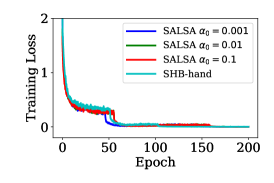
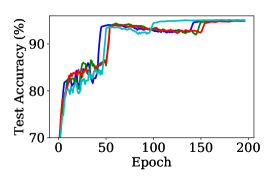
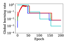
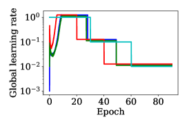
Figure 2: SALSA on CIFAR-10 (left column) and ImageNet (right column) with default parameters, starting from three different initial learning rates. The performance of SALSA matches that of a hand-tuned SHB method (SHB-hand).

We combine SSLS and SASA+ to form an autonomous algorithm called SALSA (Stochastic Approximation with Line-search and Statistical Adaptation). Figure 1 shows the typical learning rate profile generated by SALSA. It starts with a small, arbitrary learning rate $\alpha_{0}$ and uses SSLS to warm up the optimization process; once a stable learning rate $\bar{\alpha}$ is reached, it automatically switches to SASA+, which relies on online statistical tests to decrease the learning rate in a constant-and-cut (staircase) fashion.

Figure 2 shows the performance of SALSA on training ResNet18 He et al. (2016) on two different datasets: CIFAR-10 (Krizhevsky and Hinton, 2009) and ImageNet (Deng et al., 2009). We tried three small initial learning rates $\alpha_{0}\in\{0.1,0.01,0.001\}$ with SALSA. In all three cases, the SSLS phase automatically settled to a stable learning rate close to $1.0$ and switched to SASA+, which then automatically decreased the learning rate twice (each by a factor of 10) based on the online statistical test. SALSA matches the train and test performance of a hand-tuned SHB method, for which the best schedule (obtained after significant tuning) sets $\alpha_{0}=1.0$ and drops the leaning rate by a factor of 10 after every 50 and 30 epochs for CIFAR-10 and ImageNet, respectively. The learning rate profiles in the bottom row of Figure 2 are all similar to the sketch in Figure 1.

In the rest of this paper, we first present the SASA+ method in Section 2 and then the SSLS procedure in Section 3. Finally, we describe their combination into SALSA in Section 4 and conclude in Section 5.

2 The SASA+ Method

In this section, we focus on statistical methods for automatically decreasing the learning rate. This line of work goes back to Kesten (1958), who used the change of sign of the inner products of consecutive stochastic gradients as a statistical indicator of slow progress and as a trigger to decrease the learning rate (see extensions in Delyon and Juditsky, 1993). Pflug (1983, 1988) considered the dynamics of SGD with constant step size for minimizing convex quadratic functions and derived necessary conditions for the resulting dynamic process to be stationary. Most recently, Yaida (2018) derived fluctuation-dissipation relations that characterized the stationary behavior of SGD and SHB with constant learning rate and momentum. We derive a more general condition for testing stationarity that works for a much broader family of stochastic optimization methods.

We consider general stochastic optimization methods in the form of (2) with a constant learning rate:

$$x^{k+1}=x^{k}-\alpha d^{k}.$$ (6)

We assume that the stochastic search direction $d^{k}$ is generated with time-homogeneous dynamics; in particular, any additional hyperparameters involved must be constant (not depending on $k$). As an example, we consider the search directions generated by the family of Quasi-Hyperbolic Momentum (QHM) methods (Ma and Yarats, 2019):

$$\begin{split}h^{k}&=(1-\beta)g^{k}+\beta h^{k-1},\\ d^{k}&=(1-\nu)g^{k}+\nu h^{k},\end{split}$$ (7)

where $0\leq\beta<1$ and $0\leq\nu\leq 1$. With $\beta=0$ or $\nu=0$, it recovers the SGD direction (3). With $\nu=1$, (7) recovers the SHB direction (4). With $0<\beta=\nu<1$, it is equivalent to the direction of Nesterov momentum (5) (Sutskever et al., 2013; Gitman et al., 2019). We assume that the dynamics of (6), driven by the stochastic gradients $g^{k}$ through (7), are stable. Stability regions of the hyperparameters in QHM are characterized by Gitman et al. (2019).

2.1 Necessary Conditions for Stationarity

The stochastic process $\{x^{k}\}$ is (strongly) stationary if the joint distribution of any subset of the sequence is invariant with respect to simultaneous shifts in the time index (see, e.g., Grimmett and Stirzaker, 2001, Chapter 9). As a direct consequence, for any test function $\phi:\mathbf{R}^{p}\to\mathbf{R}$, we have

$$\mathbf{E}_{x^{k}\sim\pi}\bigl{[}\phi(x^{k+1})\bigr{]}=\mathbf{E}_{x^{k}\sim\pi}\bigl{[}\phi(x^{k})\bigr{]},$$ (8)

where $\pi$ denotes the stationary distribution of $\{x^{k}\}$. If $\phi$ is smooth, then we use Taylor expansion to obtain

$$\phi(x^{k+1}) =\phi(x^{k})\!-\!\alpha\bigl{\langle}\nabla\phi(x^{k}),d^{k}\bigr{\rangle}\textstyle\!+\!\frac{\alpha^{2}}{2}\bigl{\langle}\nabla^{2}\phi(x^{k})d^{k},d^{k}\bigr{\rangle}+O(\alpha^{3}).$$ (9)

Taking expectations on both sides of the above equality and applying (8), we obtain (after cancleing a common factor $\alpha$)

$$\mathbf{E}_{x^{k}\sim\pi}\Bigl{[}\bigl{\langle}\nabla\phi(x^{k}),d^{k}\bigr{\rangle}\!-\textstyle\frac{\alpha}{2}\bigl{\langle}\nabla^{2}\phi(x^{k})d^{k},d^{k}\bigr{\rangle}\Bigr{]}\!=O(\alpha^{2}).$$ (10)

For an arbitrary test function $\phi$, it is very hard in practice to compute or approximate the $O(\alpha^{2})$ term on the right-hand side. In addition, computing the Hessian-vector product $\nabla^{2}\phi(x^{k})d^{k}$ can be very costly. Therefore, we choose the simple quadratic function $\phi(x)=\frac{1}{2}\|x\|^{2}$, which results in

$$\mathbf{E}_{x^{k}\sim\pi}\left[\bigl{\langle}x^{k},d^{k}\bigr{\rangle}-\textstyle\frac{\alpha}{2}\|d^{k}\|^{2}\right]=0.$$ (11)

This condition holds exactly for any stochastic optimization method of the form (6) if it reaches stationarity. Beyond stationarity, it requires no specific assumption on the loss function or noise model for the stochastic gradients.

Yaida (2018) focused on the SHB method with direction $d^{k}=(1-\beta)g^{k}+\beta d^{k-1}$ and proposed the condition

$$\mathbf{E}_{x^{k}\sim\pi}\left[\bigl{\langle}x^{k},g^{k}\bigr{\rangle}\textstyle-\frac{\alpha}{2}\frac{1+\beta}{1-\beta}\|d^{k}\|^{2}\right]=0.$$ (12)

It can be shown that this is equivalent to a special case of (11). Condition (11) can be applied without modification to the more general QHM family (7) and other algorithms of the form (6) with time-homogeneous dynamics.

If $\{x^{k}\}$ starts with a nonstationary distribution and converges to a stationary state, we have

$$\lim_{k\to\infty}\mathbf{E}\left[\bigl{\langle}x^{k},d^{k}\bigr{\rangle}-\textstyle\frac{\alpha}{2}\|d^{k}\|^{2}\right]=0.$$ (13)

In the next section, we devise a simple statistical test to determine if condition (11) fails to hold. In this case, the learning process has not stalled, and we can continue with the same step size. If we fail to detect non-stationarity (i.e., the dynamics may be approximately stationary), we will reduce the learning rate $\alpha$ to allow for finer convergence.

Stationarity of the Loss Function. Another obvious test function one may consider is the loss function $F$ itself. Since $F(x^{k})=\mathbf{E}_{\xi}[f_{\xi}(x^{k})]$, we can test (for any $i>0$)

$$\mathbf{E}_{x^{k},\xi^{k}}\bigl{[}f_{\xi^{k}}(x^{k})\bigr{]}=\mathbf{E}_{x^{k+i},\xi^{k+i}}\bigl{[}f_{\xi^{k+i}}(x^{k+i})\bigr{]},$$ (14)

where $\xi^{k}$ is independent of $x^{k}$. We cannot use $\phi(x)=F(x)$ in (9) to derive a condition like (11), since both the Hessian and the higher order terms are hard to estimate in practice. Instead, we will derive a simple SLOPE test in the next section to detect if the training loss has a decreasing trend. As we will show in experiments, the SLOPE test does not work well for detecting stationarity for the purpose of decreasing the learning rate. However, it can be very useful to automatically switch from SSLS to SASA+ (Figure 1).

2.2 Statistical tests of (non-)stationarity

input: $x^{0}$, $\alpha_{0}$  (default parameters: $N_{\mathrm{min}}$, $K_{\mathrm{test}}$, $\delta,\theta,\tau$)

$\alpha\leftarrow\alpha_{0}$

$k_{o}\leftarrow 0$

for $k=0,...,T-1$ do

       Randomly sample ${\xi_{k}}$ and compute $d^{k}$ (e.g., using QHM)

       $x^{k+1}\leftarrow x^{k}-\alpha d^{k}$

       $\Delta_{k}\leftarrow\bigl{\langle}x^{k},d^{k}\bigr{\rangle}-\frac{\alpha}{2}\|d^{k}\|^{2}$

       $N\leftarrow\lceil\theta(k-k_{o})\rceil$

       if $N>N_{\mathrm{min}}$ and $k\!\!\mod K_{\mathrm{test}}==0$ then

             $(\hat{\mu}_{N},\hat{\sigma}_{N})\leftarrow$ statistics of $\{\Delta_{k-N+1},\ldots,\Delta_{k}\}$

            [0.5ex] if $0\in\hat{\mu}_{N}\pm t^{*}_{1-\delta/2}\frac{\hat{\sigma}_{N}}{\sqrt{N}}$ then

                   $\alpha\leftarrow\tau\alpha$

                   $k_{o}\leftarrow k$

             end if

            

       end if

      

end for

output: $x^{T}$ (or the average of last epoch)

Algorithm 1 SASA+

In order to test if the stationarity condition (11) holds approximately, we collect the simple statistics

$$\Delta_{k}~{}\triangleq~{}\textstyle\bigl{\langle}x^{k},d^{k}\bigr{\rangle}-\frac{\alpha}{2}\|d^{k}\|^{2}.$$

In the language of hypothesis testing (e.g., Lehmann and Romano, 2005), we make as our null hypothesis that the dynamics (6) have reached a stationary distribution $\pi$. If we have $N$ samples $\{\Delta_{k}\}$, we know from equation (11) and the Markov chain CLT (see its application in Jones et al. (2006)) that as $N\to\infty$, under the null hypothesis, the mean statistic $\bar{\Delta}$ follows a normal distribution with mean 0 and variance $\sigma_{\Delta}^{2}/\sqrt{N}$. Our alternative hypothesis is that the dynamics (6) have not reached stationarity.

To test these hypotheses, we adopt the classical confidence interval test. We use the most recent $N$ samples $\{\Delta_{k-N+1},\ldots,\Delta_{k}\}$ to compute the sample mean $\hat{\mu}_{N}$ and a variance estimator $\hat{\sigma}_{N}^{2}$ for $\sigma_{\Delta}^{2}$. Then we form the $(1\!-\!\delta)$-confidence interval $(\hat{\mu}_{N}-\omega_{N},~{}\hat{\mu}_{N}+\omega_{N})$ with half width

$$\omega_{N}=t^{*}_{1-\delta/2}\frac{\hat{\sigma}_{N}}{\sqrt{N}},$$ (15)

where $t_{1-\delta/2}^{*}$ is the $(1-\delta/2)$ quantile of the Student’s $t$-distribution with degrees of freedom corresponding to that in the variance estimator $\hat{\sigma}_{N}^{2}$. Because the sequence $\{\Delta_{k-N+1},\ldots,\Delta_{k}\}$ are highly correlated due to the underlying Markov dynamics, the classical formula for the sample variance (obtained by assuming i.i.d. samples) does not work for $\hat{\sigma}_{N}^{2}$ (causing too small confidence intervals). We need to use more sophisticated batch mean (BM) or overlapping batch mean (OLBM) variance estimators developed in the Markov chain Monte Carlo literature (e.g., Jones et al., 2006; Flegal and Jones, 2010). See Lang et al. (2019) for detailed explanation. We also list the formulas for computing BM and OLBM in Appendix A.2.

If the confidence interval in (15) contains $0$, we fail to reject the null hypothesis that the learning process is at stationarity, which means the learning rate should be decreased. Otherwise, we accept the alternative hypothesis of non-stationarity and keep using the current constant learning rate. Algorithm 1 summarizes our new method called SASA+, and Table 1 lists its hyperparameters and their default values.

Table 1: List of hyperparameters of Algorithm 1

Parameter	Explanation	Default value
$N_{\textrm{min}}\in\mathbb{Z}_{+}$	minimum # of samples for testing	$\min\{1000,\lceil n/b\rceil\}$
$K_{\textrm{test}}\in\mathbb{Z}_{+}$	period to perform statistical test	$\min\{100,\lceil n/b\rceil\}$
$\delta\in(0,1)$	$(1\!-\!\delta)$-confidence interval	0.05
$\theta\in(0,1)$	fraction of recent samples to keep	$1/8$
$\tau\in(0,1)$	learning rate drop factor	$1/10$
where $n$ is total number of training examples and $b$ is the mini-batch size.

Our method is an extension of SASA (Statistical Adaptive Stochastic Approximation) proposed by Lang et al. (2019), which is based on testing the condition (12) for the SHB dynamics only. In addition to using a much more general stationarity condition (11), another major difference is that they set non-stationarity as the null hypothesis and stationarity as the alternative hypothesis (opposite to ours). This leads to a more complex “equivalence test” that requires an additional hyperparameter (see Appendix B). Our test is simpler, more intuitive, and computationally as robust.

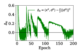
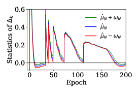
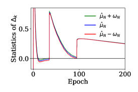
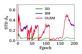
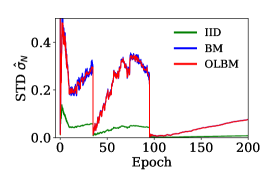
Figure 3: Statistics in SASA+. The two columns are from runs with drop ratio $\tau=1/2$ and $1/10$ respectively. The top row shows the instantaneous value of $\Delta_{k}$. The middle row shows the confidence interval of $\mathbf{E}[\Delta_{k}]$, which contains 0 with high probability if the process is stationary. The bottom row shows the variance estimated by different methods: i.i.d. formula, BM and OLBM estimators.

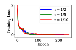
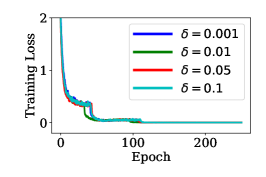
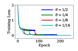
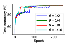
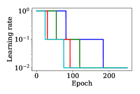
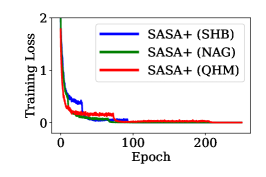
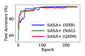
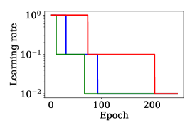
Figure 4: Sensitivity analysis of SASA+ on CIFAR10. The test accuracy and learning rate schedule for SASA+ using different values of $\tau$ (first row), $\delta$ (second row) and $\theta$ (third row) around the default values in Table 1; SASA+ applied on different methods (i.e., SHB, NAG and QHM) (last row).

SLOPE test for training loss. Here we describe a statistical test that aims to detect if the training loss is no longer decreasing. As the training goes on, we collect the minibatch loss $f_{\xi^{k}}(x^{k})$ at every iteration, and build a linear model based on the last $N$ mini-batches $\{(i,f_{\xi^{i}}(x^{i}))\}_{i=k-N+1}^{k}$. We denote this linear model as $\hat{f}_{\xi^{i}}(x^{i})=c_{0}+c_{1}k$, and propose to use the following one-sided test

$$\mbox{null}:c_{1}\geq 0\quad\mbox{vs.}\quad\mbox{alternative}:c_{1}<0.$$ (16)

Like in SASA+, if we reject the null hypothesis with high confidence, then we keep the learning rate; Otherwise, we decrease the learning rate by a constant factor. We use the standard t-test for linear regression (e.g., Montgomery et al., 2012, Section 2.3). Specifically, we first compute the estimators $\hat{c}_{0}$ of $c_{0}$ and $\hat{c}_{1}$ of $c_{1}$ by solving a least-squares problem, then compute a statistic $t_{\text{slope}}=\hat{c}_{1}/\sqrt{\hat{\sigma}_{f}}$, where $\hat{\sigma}_{f}$ can be computed with standard formula which we provide in Appendix A.3. When $f_{\xi_{i}}(x_{i}))\!=\!c_{0}\!+\!\zeta_{i}$ with i.i.d. Gaussian noises $\zeta_{i}$, the statistic $t_{\text{slope}}$ follows the $t$-distribution with $N\!-\!2$ degrees of freedom. Given a confidence level $(1\!-\!\delta$), we reject the null if $t_{\text{slope}}\!<\!t_{\delta,N-2}$ and accept it otherwise.

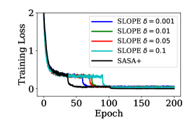
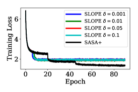
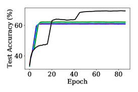
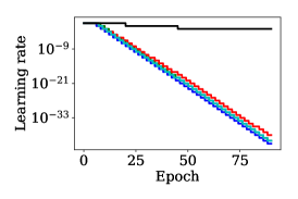
Figure 5: Comparison of SLOPE test with different confidence level $\delta$ and the default run of SASA+. First column: CIFAR-10 with ResNet18. Second column: ImageNet with ResNet18.

2.3 SASA+ Experiments

Figure 3 shows the evolution of SASA+’s different statistics during training the ResNet18 model on CIFAR-10 using the default parameters in Table 1. Between two jumps, the statistics $\Delta_{k}$ decays toward zero. As long as its confidence interval (15) does not overlap with 0, we are confident that the process is not stationary yet and keep training with the current learning rate. Otherwise, we decrease the learning rate and enter another cycle of approaching stationarity.

Figure 4 illustrates the sensitivity of SASA+ to its hyperparameters around their default values. The first row shows that SASA+ is robust to the choice of the dropping factor $\tau$. The larger $\tau$ is, the longer the process will stay between two drops (also see Figure 3). The second row shows SASA+ is insensitive to the confidence level $\delta$. The third row shows the effect of $\theta$, the fractions of samples to keep after reset. Smaller $\theta$ values lead to more frequent dropping, but do not impact the final performance. The fourth row shows that SASA+ can work with various algorithms, i.e., SHB (4), NAG (5) and QHM (7). Results on ImageNet and MNIST in Appendix C.2 also support these findings.

Figure 5 shows that the SLOPE test is too aggressive after the first learning rate drop, and thus cannot reach good training loss and testing accuracy. See similar results for logistic regression on MNIST in Appendix C.3.

3 Smoothed Stochastic Line Search

input: $x^{0}$, $\alpha_{0}$

parameters: $c\in(0,1/2)$, $\rho_{\mathrm{inc}}\geq 1$, $\rho_{\mathrm{dec}}\in(0,1)$, $m>0$

for $k=0,...,T-1$ do

       Sample ${\xi_{k}}$, compute $g^{k}\leftarrow\nabla f_{{\xi_{k}}}(x^{k})$ and $d^{k}$

       $\eta_{k}\leftarrow\rho_{\mathrm{inc}}\alpha_{k-1}$

       for $i=1,\ldots,m$ do

             if $f_{{\xi_{k}}}(x^{k}-\eta_{k}g^{k})<f_{{\xi_{k}}}(x^{k})-c\cdot\eta_{k}\|g^{k}\|^{2}$ then

                   break (out of for loop)

            else

                   $\eta_{k}\leftarrow\rho_{\mathrm{dec}}\eta_{k}$

             end if

            

       end for

      $\alpha_{k}\leftarrow(1-\gamma)\alpha_{k-1}+\gamma\eta_{k}$

       $x^{k+1}\leftarrow x^{k}-\alpha_{k}d^{k}$

end for

output: $x^{T}$

Algorithm 2 Smoothed Stochastic Line-Search (SSLS)

SASA+ can automatically decrease the learning rate to refine the last phase of the optimization process, but it relies on an appropriate initial learning rate to make fast progress. The appropriate initial learning rate varies substantially for different objective functions, machine learning models, and training datasets. Setting it appropriately without expensive trial and error is a major challenge for all stochastic gradient methods, adaptive or not.

Several recent works (e.g., Schmidt et al., 2017; Vaswani et al., 2019) explore the use of classical line-search schemes (e.g., Nocedal and Wright, 2006, Chapter 3) for stochastic optimization. One of the main difficulties is that the estimated step sizes may vary a lot from step to step and it may not capture the right step size for the average loss function. To overcome this difficulty, we propose a smoothed stochastic line-search (SSLS) procedure listed in Algorithm 2.

During each step $k$, SSLS uses the classical Armijo line-search (e.g., Nocedal and Wright, 2006, Chapter 3) to find a step size $\eta_{k}$ for the randomly chosen function $f_{{\xi_{k}}}$ (initialized by $\alpha_{k-1}$), then sets the next learning rate to be

$$\alpha_{k}=(1-\gamma)\alpha_{k-1}+\gamma\eta_{k},$$

where $\gamma\in[0,1]$ is a smoothing parameter. When $\gamma=1$, SSLS reduces to the stochastic Armijo line-search used by Vaswani et al. (2019). For optimization over a finite dataset, a good choice is to set $\gamma=b/n$ where $n$ is the total number of training examples and $b$ is the mini-batch size. Suppose $\rho_{\mathrm{inc}}=2$ and $\eta_{k}=2\alpha_{k-1}$ is accepted at step $k$, then $\alpha_{k}=(1-\gamma)\alpha_{k-1}+\gamma(2\alpha_{k-1})=(1+\gamma)\alpha_{k-1}.$ If this happens at every iteration over one epoch (of $\lceil n/b\rceil$ iterations) and $n\gg b$, then

$$\alpha_{k+\lceil n/b\rceil}=(1+b/n)^{\lceil n/b\rceil}\alpha_{k}\approx e\cdot\alpha_{k}.$$ (17)

Therefore, the most aggressive growth of the learning rate is by a factor of $e$ over one epoch. Such a growing factor is reasonable for line search in deterministic optimization (e.g., Nesterov, 2013). Setting $\gamma=\sqrt{b/n}$ leads to maximum growth of $e^{2}$ over one epoch. A similar smoothing effect holds for decreasing the learning rate as well. The smoothing scheme allows us to use standard increasing and decreasing factors, and we use $\rho_{\mathrm{inc}}=2$, $\rho_{\mathrm{dec}}=1/2$, $c=0.05$, and $\gamma=\sqrt{b/n}$ as the default parameters.

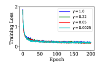
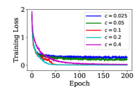
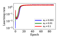
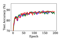
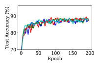
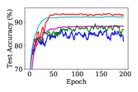
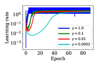
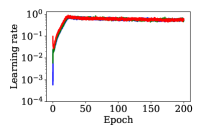
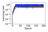
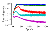
(a)                                    (b)                                    (c)                                    (d)

Figure 6: Sensitivity of SSLS around its default values $c=0.05$ and $\gamma=\sqrt{b/n}$ (0.05 for CIFAR-10 and 0.01 for ImageNet). (a) Initial learning rate $\alpha_{0}$, (b) The smoothing factor $\gamma$ and (c) and the sufficient decrease constant $c$ on CIFAR-10 with ResNet18. The column (d) shows the learning rate schedules of SSLS when applied to ImageNet with ResNet18 with different hyperparameters. Best viewed in color.

Following the analysis of Armijo line-search in Vaswani et al. (2019), it is possible to show that SSLS has similar convergence properties under the smooth and interpolation assumptions, which we leave as a future research project. In this paper, we are mainly interested in its performance as a practical heuristic. In particular, we use it on deep neural network models with ReLU activations. Here the loss functions are non-smooth, and classical theoretical analysis for line-search do not carry over. Nevertheless, we found SSLS to have robust performance in all of our experiments. In order to handle the case of potential non-descent directions in the non-smooth case, we always exit the line search after a maximum of $m$ tries. By default, we set $m=2$ (there is no significant difference from $m=2$ to $m=10$).

SSLS Experiments. Figure 6 shows our sensitivity study on SSLS. Column (a) and (b) indicate that for a wide range of the initial learning rate $\alpha_{0}$ and the smoothing parameter $\gamma$, SSLS always settles down to a stable learning rate ($0.53$ for CIFAR-10 and $2.1$ for ImageNet, which is comparable with the best hand-tuned value of 1.0). However, large $\gamma$ causes oscillation around a stable learning rate. Column (c) shows that the larger the sufficient descent constant $c$ is, the smaller the stable learning rate is and the slower SSLS reaches it. This is intuitive because larger $c$ requires steeper descent, forcing SSLS to settle on a smaller learning rate on average. Note that both training loss and validation accuracy obtained by SSLS is worse than the results obtained by hand-tuned optimizers. Column (d) shows the resulting learning rates of SSLS on ImageNet, with more details in Appendix C.4.

4 SALSA

input: $x^{0}\in\mathbf{R}^{p}$, $\alpha_{0}>0$, $switched$=False

for $k=0,...,T$ do

       if not $switched$ then

             Run one step of SSLS (Algorithm 2)

             $x\_stationary\leftarrow$ SASA+ test in Algorithm 1

             $f\_stationary\leftarrow$ SLOPE test (16)

             $switched\leftarrow$ $x\_stationary$ or $f\_stationary$

      else

             Run one step of SASA+ (Algorithm 1)

       end if

      

end for

output: $x^{T}$

Algorithm 3 SALSA: SASA+ with warmup by SSLS

Finally, we combine SSLS with SASA+ to form Algorithm 3, which we call SALSA (Stochastic Approximation with Line-search and Statistical Adaption). Without prior knowledge of the loss function and training dataset, we start with a very small learning rate and use SSLS to gradually increase it to be around a stationary value that is (automatically) customized to the problem, as shown in Figure 6. At every $K_{\text{test}}$ iterations, SALSA performs the stationary test in SASA+ (Algorithm 1) and the SLOPE test (16), to determine whether the dynamics become stationary and whether the training loss is still decreasing, respectively. If either form of stationarity is detected, SALSA switches from SSLS to SASA+. After the switch, SASA+ takes over the learning rate scheduling and finishes the training. The SLOPE test proves to be very effective in detecting whether the training loss is still decreasing, which prevents the learning rate growing too large (but not as effective in reducing the learning rate afterwards, as shown in Section 2.3)

Computational overhead of SALSA. When we fix the number of training epochs, the wall-clock time of SSLS is at most 1.5 times of that of without using line search. This 0.5x overhead is due to the at most 3 extra function evaluations in each line search step (with $m=2)$. Notice that line search is performed on the same minibatch and only needs the function value (not the gradient). In SALSA, SSLS typically switches to SASA+ in less than one-third of the total training epochs. Therefore, the total overhead of using SSLS is typically only 0.15 that of the total time without SSLS. The overhead of SASA+ is the same as that of SASA (Lang et al., 2019), which is negligible in practice.

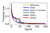
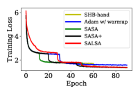
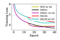
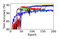
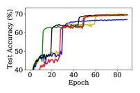
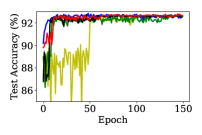
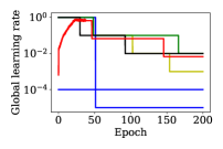
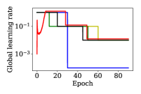
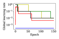
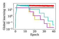
Figure 7: Comparison of different optimizers on CIFAR-10 with ResNet18 (first column), ImageNet with ResNet18 (second column), MNIST with a linear model (third column) and Wikitext-2 with LSTM (fourth column). SALSA starts from an small, arbitrary learning rate while other methods start with a hand-tuned initial learning rate. In Column (d), “w/ val” means decreasing the learning rate when the validation loss stops improving (or the statistical test fires, whichever comes first). Best viewed in color.

SALSA Experiments. In Figure 7, we evaluate the performance of SALSA with experiments on four popular datasets. We compare SALSA to the following baselines: SHB with a hand-tuned constant-and-cut learning rate schedule (SHB-hand), Adam Kingma and Ba (2014) with a tuned warmup phase (Adam w/ warmup) (e.g., Wilson et al., 2017), SASA from Lang et al. (2019), and our SASA+. SALSA starts from a small, arbitrary learning rate while all other methods start with a hand-tuned initial learning rate. We showed in Figure 2 that for both CIFAR-10 and ImageNet, SALSA can start with an arbitrary small initial learning rate and obtain training and testing performance that are on par with that of a hand-tuned optimizer. Figure 9 in Appendix C.1 shows that this is also true for the MNIST and Wikitext-2 datasets. Unless otherwise stated, we use the default values in Table 1 for hyperparameters in SASA+ and SALSA.

CIFAR-10. With random cropping and random horizontal flipping for data augmentation, one can train a modified ResNet18 model (with weight decay $0.0005$) using a hand-tuned optimizer (SHB-hand) to achieve testing accuracy of 95% (Liu, 2019). Using a tuned $\alpha_{0}=1e^{-4}$ (by grid search), Adam is only able to reach around 92.5% for the same model. With an additional “warmup” phase of 50 epochs, “Adam w/ warmup” can achieve 94.5% test accuracy. In contrast, both SASA+ and SALSA are able to reach test accuracy similar to SHB-hand. While other methods starts from a hand-tuned initial learning rate of $1.0$, SALSA starts from a small initial learning rate of $0.01$.

ImageNet. On the large scale ImageNet dataset (Deng et al., 2009), we use the ResNet18 architecture, random cropping and random horizontal flipping for data augmentation, and weight decay $0.0001$. Column (b) in Figure 7 compares the performance of the different optimizers. Even with a hand-tuned $\alpha_{0}=1e^{-4}$ and allowed to have a long warmup phase (30 epochs), “Adam w/ warmup” fails to match the testing accuracy of the hand-tuned SHB. On the other hand, both SASA+ and SALSA are able to match the best performance.

MNIST. We train a linear model (logistic regression) on the MNIST dataset. Column (c) in Figure 7 shows that, for this simple convex optimization problem, all methods finally achieve similar performance.

Wikitext-2. We train the PyTorch word-level language model example (PyTorch, 2019) on the Wikitext-2 dataset (Merity et al., 2016). We use 1500-dimensional embeddings, 1500 hidden units, tied weights, and dropout 0.65, and also gradient clipping with threshold 0.25. We compare against SGD with a learning rate tuned using a validation set. This baseline starts with a hand-tuned initial learning rate of $\alpha_{0}=20$ and drops the learning rate by a factor of 4 when the validation loss stops improving. Column (d) of Figure 7 shows that SASA (Lang et al., 2019), SASA+ and SALSA all overfit to the training loss in this case. We tried to combine them with the validation heuristic, so we drop the learning rate if the statistical test fires or the validation loss stops decreasing (yet another statistical test!), whichever comes first. This combination (shown as “SASA+ w/val” and “SALSA w/val”) largely closes the gap in testing performance between SALSA and “SGD w/val.”

5 Conclusions

We presented SASA+, a simpler, yet more powerful variant of the statistical adaptive stochastic approximation (SASA) method proposed by Lang et al. (2019). SASA+ uses a single condition for (non-)stationarity that works without modification for a broad family of stochastic optimization methods. This greatly simplifies its implementation and deployment in software packages. While SASA+ focuses on how to automatically reduce the learning rate to obtain better asymptotic convergence, we also propose a smoothed stochastic line-search (SSLS) method to warm up the optimization process, thus removing the burden of expensive trial and error for setting a good initial learning rate. The combined algorithm, SALSA, is highly autonomous and robust to different models and datasets. Using the same default settings, SALSA obtained state-of-the-art performance on several common deep learning models that is competitive with the best hand-tuned optimizers.

In general, we believe that statistical tests are powerful tools that should be exploited further in stochastic optimization, especially for making the training of large-scale machine learning models more autonomous and reliable.

Appendix A More details on statistical tests

A.1 From the master equation in SASA+ to that in Yaida [2018] and Lang et al. [2019]

Proposition 1.

When the dynamics of $(x^{k},g^{k},d^{k})$ is given by the stochastic heavy ball method, i.e., (2) and (4), the master equation in SASA+, i.e.,

$$\mathbf{E}_{(x^{k},g^{k},d^{k})\sim\pi}\left[\bigl{\langle}x^{t},d^{t}\bigr{\rangle}-\textstyle\frac{\alpha}{2}\|d^{t}\|^{2}\right]=0\quad\forall t\geq k$$ (18)

and the stationarity of $\|d^{k}\|^{2}$ together lead to the master equation in Yaida [2018], i.e.,

$$\mathbf{E}_{(x^{k},g^{k},d^{k})\sim\pi}\left[\bigl{\langle}x^{t},g^{t}\bigr{\rangle}\textstyle-\frac{\alpha}{2}\frac{1+\beta}{1-\beta}\|d^{t}\|^{2}\right]=0\quad\forall t\geq k+1.$$ (19)

Here, $(x^{k},g^{k},d^{k})\sim\pi$ means that the dynamics of $(x^{k},g^{k},d^{k})$ reaches its stationary distribution $\pi$ at time $k$.

Proof.

To avoid cumbersome subscripts, we simply write $\mathbf{E}_{(x^{k},g^{k},d^{k})\sim\pi}$ as $\mathbf{E}$ in the proof. For any $t\geq k+1$, from SASA+’s master equation, we have

$$\mathbf{E}\left[\bigl{\langle}x^{t},d^{t}\bigr{\rangle}-\textstyle\frac{\alpha}{2}\|d^{t}\|^{2}\right] =0,$$

$$\mathbf{E}\left[\bigl{\langle}x^{t},d^{t-1}\bigr{\rangle}+\textstyle\frac{\alpha}{2}\|d^{t-1}\|^{2}\right] =0.$$

Then we have

$$\frac{\alpha}{2}\mathbf{E}[\|d^{t}\|^{2}]=\mathbf{E}\left[\bigl{\langle}x^{t},(1-\beta)g^{t}+\beta d^{t-1}\bigr{\rangle}\right]$$

$$=(1-\beta)\mathbf{E}\left[\bigl{\langle}x^{t},g^{t}\bigr{\rangle}\right]+\beta\mathbf{E}\left[\bigl{\langle}x^{t},d^{t-1}\bigr{\rangle}\right]$$

$$=(1-\beta)\mathbf{E}\left[\bigl{\langle}x^{t},g^{t}\bigr{\rangle}\right]-\beta\frac{\alpha}{2}\mathbf{E}\left[\|d^{t-1}\|^{2}\right]$$

Thanks to the stationarity of $\|d^{t}\|^{2}$ (i.e., $\mathbf{E}[\|d^{t}\|^{2}]=\mathbf{E}[\|d^{t+1}\|^{2}]$ for $t\geq k$), we obtain Equation (19), i.e., the master equation in Yaida [2018]. ∎

In fact, when the dynamics of $(x^{k},g^{k},d^{k})$ is given by the stochastic heavy ball method, i.e., (2) and (4), one can verify the following identity for any $k\geq 1$:

$$\bigl{\langle}x^{k},g^{k}\bigr{\rangle}\textstyle-\frac{\alpha}{2}\frac{1+\beta}{1-\beta}\|d^{k}\|^{2}$$ (20)

$$= \frac{1}{2\alpha(1-\beta)}\big{(}(\beta\|x^{k}\|^{2}-\|x^{k+1}\|^{2}-\alpha^{2}\beta\|d^{k}\|^{2})$$

$$-(\beta\|x^{k-1}\|^{2}-\|x^{k}\|^{2}-\alpha^{2}\beta\|d^{k-1}\|^{2})\big{)}.$$

Therefore, the master equation in Yaida [2018] is taking a test function

$$\phi(\{x^{k},g^{k},d^{k}\})=\beta\|x^{k}\|^{2}-\|x^{k+1}\|^{2}-\alpha^{2}\beta\|d^{k}\|^{2}.$$ (21)

The tests in Yaida [2018] and Lang et al. [2019] are essentially testing whether $\phi(\{x^{k},g^{k},d^{k}\})$ in (21) reaches stationarity or not.

A.2 MCMC variance estimators

Several estimators for the asymptotic variance of the history-average estimator of a Markov chain have appeared in work on Markov Chain Monte Carlo (MCMC). Jones et al. [2006] gives a nice example of such results. Here we simply list two common variance estimators, and we refer the reader to that work and Lang et al. [2019] (from which we borrow notation) for appropriate context and formality.

Batch Means (BM) variance estimator.

Let $\bar{z}_{N}$ be the history average estimator with $N$ samples, that is, given samples $\{z_{i}\}$ from a Markov chain, $\bar{z}_{N}=\frac{1}{N}\sum_{i=i_{0}}^{i_{0}+N}z_{i}$. Now form $p$ batches from the $N$ samples, each of size $q$. Compute the “batch means” $\bar{z}^{j}=\frac{1}{q}\sum_{i=jq}^{(j+1)q-1}z_{i}$ for each batch $j$. Then compute the batch means estimator using:

$$\hat{\sigma}_{N}^{2}=\frac{q}{p-1}\sum_{j=0}^{p-1}(\bar{z}^{j}-\bar{z}_{N})^{2}.$$ (22)

The estimator is just the variance of the batch means around the history average $\bar{z}_{N}$. This statistic has $p-1$ degrees of freedom. As in Jones et al. [2006] and Lang et al. [2019], we take $p=q=\sqrt{N}$ when using this estimator.

Overlapping batch means variance estimator.

The overlapping batch means (OLBM) estimator Flegal and Jones [2010] has better asymptotic variance than the batch means estimator. The OLBM estimator is conceptually the same, but it uses $N-p+1$ overlapping batches of size $p$ (rather than disjoint batches) and has $N-p$ degrees of freedom. It can be computed as:

$$\hat{\sigma}_{N}^{2}=\frac{Np}{(N-p)(N-p+1)}\sum_{j=0}^{N-p}(\bar{z}_{N}-\frac{1}{p}\sum_{i=1}^{p}z_{j+i})^{2}.$$ (23)

In practice, there is not much difference between using the BM or the OLBM estimators in SASA+.

A.3 Slope test for linear regression

For the SLOPE test presented in Section 2.2, the formulas for the statistic are given by

$$t_{\text{slope}} =\hat{c}_{1}/\sqrt{\hat{\sigma}_{f}},$$ (24)

$$\hat{\sigma}_{f}^{2} =\frac{\textstyle\sum_{i=k-N+1}^{k}(f_{\xi_{i}}(x_{i})-\hat{f}_{\xi_{i}}(x_{i}))^{2}}{\textstyle\sum_{i=k-N+1}^{k}(i-\overline{i})^{2}}$$

where $\overline{i}=\frac{1}{N}\sum_{i=k-N+1}^{k}i$ is the center of the regressor $i$. See, for example, Montgomery et al. [2012, Section 2.3] for further details.

Appendix B The statistical tests in SASA and SASA+

As mentioned in our contributions, there are two main differences between SASA from Lang et al. [2019] and SASA+. First, SASA+ has a much more general “master stationary condition” (11), so it can be applied to any stochastic optimization method with constant hyperparameters (e.g., SGD, stochastic heavy-ball, NAG, QHM, etc.), while the stationary condition in Yaida (2018) and SASA proposed in Lang et al. [2019] (see Equation (12)) only applies to the stochastic heavy-ball method. Second, the statistical tests used in SASA and SASA+ are quite different, as we elaborate below.

The difference starts from a conceptual change from SASA to SASA+. In SASA, one wants to confidently detect stationarity. If stationarity is detected, one decreases the learning rate, and otherwise keeps it the same. In SASA+, one wants to confidently detect non-stationarity. If non-stationarity is detected, one keeps the learning rate the same, and otherwise decreases. This conceptual change leads to a simpler and more rigorous statistical test in SASA+.

B.1 Equivalence test in SASA

To confidently detect stationarity, SASA has to set non-stationarity as null hypothesis and stationarity as the alternative hypothesis. If one confidently rejects the null (non-stationarity), then one can be confident that the process is stationarity. Instead of detecting stationarity, SASA simplifies to only detect the necessary but not sufficient stationarity condition (12). Formally, the test in SASA is

$$H_{0}:\mathbf{E}[\Delta]\neq 0\qquad\mbox{ vs. }\qquad H_{1}:\mathbf{E}[\Delta]=0,$$ (25)

where samples of $\Delta$, i.e., $\Delta_{k}\triangleq\bigl{\langle}x^{k},d^{k}\bigr{\rangle}-\frac{\alpha}{2}\|d^{k}\|^{2}$, are collected along the training process. This kind of test is called an equivalence test in statistics, see, e.g., Streiner [2003]. There is no power in the equivalence test (25), i.e., one cannot confidently reject the null hypothesis and prove stationarity at all! Intuitively, even when the process is stationary, with only a finite number of (noisy) samples $\{\Delta_{k}\}_{k=0}^{N_{1}}$, the sample mean $\bar{\Delta}_{N}\neq 0$ (with probability one) is always more likely to be the true mean than the singleton $0$. In other words, one can not deny that the process is probably infinitely close to stationary but still non-stationary.

To gain power in the equivalence test, one needs to use domain knowledge to define an equivalence interval. Formally, the true test in SASA is

$$H_{0}:|\mathbf{E}[\Delta]|>\zeta\nu\qquad\mbox{ vs. }\qquad H_{1}:\mathbf{E}[\Delta]\in[-\zeta\nu,\zeta\nu],$$ (26)

where $\zeta\nu$ is the equivalence interval. In English, instead of the usual null hypothesis of not-equal-to-zero in (25), now the null hypothesis is not-equal-to-zero by a margin $\zeta\nu$. In this case, when $\mathbf{E}[\Delta]$’s confidence interval is contained in the equivalence interval, i.e.,

$$\biggl{[}\bar{\Delta}_{N}-t_{1-\delta/2}^{*}\frac{\hat{\sigma}_{N}}{\sqrt{N}},~{}\bar{\Delta}_{N}+t_{1-\delta/2}^{*}\frac{\hat{\sigma}_{N}}{\sqrt{N}}\biggr{]}\subset[-\zeta\bar{\nu}_{N},\zeta\bar{\nu}_{N}].$$ (27)

we are confident to reject the null hypothesis and to prove/accept $H_{1}$ (the stationary condition is met within an error tolerance). This is exactly the test in SASA Lang et al. [2019], see its Equation (10). However, this equivalence test requires estimation of $\bar{\nu}_{N}$ (that estimates the magnitude of $\Delta$) and an additional hyperparameter $\zeta$ that controls the equivalence interval width. In SASA’s notation, the equivalence width $\zeta$ is denoted by $\delta$.

Moreover, SASA makes the unjustified assumption that under their null hypothesis ($H_{0}:|\mathbf{E}[\Delta]|>\zeta\nu$), the Markov central limit theorem holds. Under their $H_{0}$, the process is non-stationary, while the construction of $\mathbf{E}[\Delta]$’s confidence interval in Eqn. (27) relies on the (asymptotic) stationarity of the Markov process. Therefore, despite the empirical success of SASA, its statistical test is intrinsically flawed because of this testing setup.

B.2 Standard test in SASA+

In SASA+, we want to confidently detect non-stationarity. If non-stationarity is detected, one keeps the learning rate the same, and otherwise one decreases it. This conceptual change naturally removes the complication of the equivalence test and the intrinsic flaw in SASA.

To confidently detect non-stationarity, SASA+ sets stationarity as the null hypothesis and non-stationarity as the alternative:

$$H_{0}:\mbox{The process is staionary}\quad\mbox{ vs. }\quad H_{1}:\mbox{The process is not staionary}.$$ (28)

The master stationary condition $\mathbf{E}[\Delta]=0$ is a necessary condition for stationary of the process, and thus confidently rejecting $\mathbf{E}[\Delta]=0$ is sufficient to confidently reject the null (stationarity) hypothesis. Moreover, under this null hypothesis, the Central Limit Theorem of Markov Processes exactly holds true (because the process is stationary), validating the construction of $\mathbf{E}[\Delta]$’s confidence interval. Therefore, the intrinsic flaw in SASA is naturally solved in SASA+.

Now we describe the test in SASA+. When the confidence interval of $\mathbf{E}[\Delta]$ does not contain $0$, i.e.,

$$0\not\in\biggl{[}\bar{\Delta}_{N}-t_{1-\delta/2}^{*}\frac{\hat{\sigma}_{N}}{\sqrt{N}},~{}\bar{\Delta}_{N}+t_{1-\delta/2}^{*}\frac{\hat{\sigma}_{N}}{\sqrt{N}}\biggr{]},$$ (29)

then we reject the null (stationary) hypothesis and keep the learning rate the same. Otherwise, we decrease the learning rate. Notice that there is no additional hyperparameter $\zeta$.

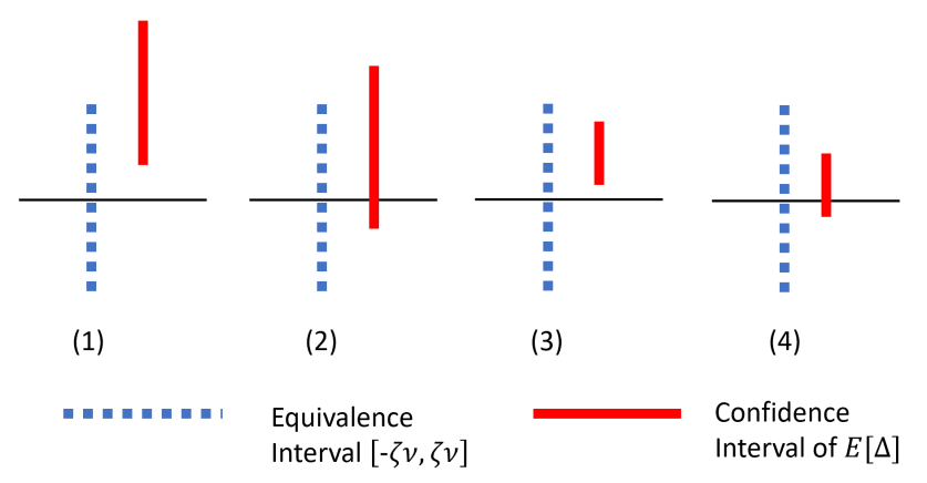
Figure 8: Statistical tests in SASA and SASA+. Case (1): both SASA and SASA+ keep the learning rate. Case (4): both SASA and SASA+ decrease the learning rate. Case (2): SASA keeps the learning rate while SASA+ decreases. Case (3): SASA decreases the learning rate while SASA+ keeps.

B.3 The difference in practice

Although SASA and SASA+ are conceptually quite different, they both use the same confidence interval (see (27) and (29)) for $\mathbf{E}[\Delta]$. In practice, their difference is illustrated in Figure 8. Their difference lies in Case (2) and (3). In Case (3), the process has not reached stationarity yet with high probability, according to the confidence interval of $\mathbf{E}[\Delta]$ (Red). SASA+’s test is confident to reject its (stationary) null hypothesis, so it keeps the learning rate the same. However, SASA decreases its learning rate because it is confident that the stationary condition holds true within its error tolerance (equivalence interval). In this case, SASA makes an error due to its relatively large equivalence interval. In Case (2), SASA+’s test is not confident to reject its (stationary) null hypothesis and so it decreases its learning rate. On the contrary, SASA’s test is not confident to claim that the stationary condition holds true within its error tolerance and thus keeps its learning rate. In this sense, SASA+ is more aggressive than SASA in decreasing learning rate.

In numerical experiments on the CIFAR10 and ImageNet datasets, the (width of) the equivalence interval $\zeta\nu$ is typically much smaller than the (width of) the confidence interval of $\mathbf{E}[\Delta]$, see Figure 5(a), 7(a) and 9(a) in Lang et al. [2019]. Notice that in those figures, the yellow curve is $\nu$ instead of $\zeta\nu$, and thus the equivalence interval is even smaller. Therefore, Case (3) happens very rarely in those experiments, and this explains the reason why SASA does not make obvious mistakes in decreasing the learning rate. In practice, Case (2) sometimes happens, and thus we can see that SASA+ seems to be slightly more aggressive at decreasing the learning rate than SASA. For example in Figure 7, the black curve (SASA+) is faster at decreasing the learning rate than the green curve (SASA).

Appendix C More experimental results

C.1 More results for SALSA

In Figure 2, we showed that for both CIFAR-10 and ImageNet, SALSA can start with a small initial learning rate and the training dynamics and final performance are the same as when it starts with a hand-tuned initial learning rate. Here, in Figure 9, we show that the same holds true for SALSA on MNIST and Wikitext-2 datasets.

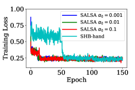
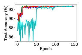
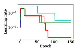
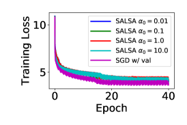
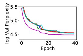
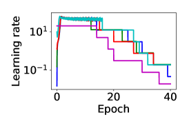
Figure 9: “SALSA” on MNIST (top row) and “SALSA w/ val” Wikitext-2 (bottom row) with default parameters, starting from three different initial learning rates. The performance of SALSA is competitive with the state-of-the-art results reported in the literature.

When SALSA with the default parameter is applied to the task of LSTM on Wikitext-2 (Figure 9, bottom), the stable learning rate obtained by the SSLS, i.e., around 45, is larger than the hand-tuned initial learning rate 20. This larger initial learning rate results in the small gap between “SALSA w/ val” and “SGD w/ val” in terms of the final perplexity on the validation dataset. To verify this, we show “SALSA w/ val” with different $c$’s ($c=0.025,0.05,0.1,0.2$) in Figure 10. The larger the $c$ is, the smaller the stable learning rate SSLS reaches. For $c=0.1$ and $0.2$ (larger than the default $0.05$), the stable learning rates obtained by SSLS are nearly the same with the hand-tuned initial learning rate, and there is no performance gap between “SALSA w/ val” and “SGD w/ val” in terms of the final validation perplexity.

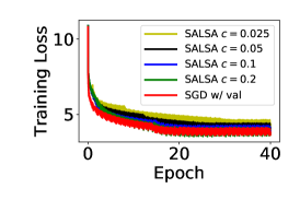
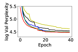
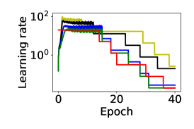
Figure 10: RNN: “SALSA w/ val” with different sufficient descent constant $c$.

C.2 More results for SASA+

In Figure 4, we show the sensitivity analysis of SASA+ on the CIFAR-10 dataset, by showing the testing accuracy and learning rate schedule. Here, in Figure 11, we provide the full sensitivity analysis, including the drop factor $\tau$ (first row), the test confidence parameter $\delta$ (second row), the ratio of recent samples to keep $\theta$ (third row), the test frequency $K_{\textrm{test}}$ (fourth row), and combined with different methods (last row). Notice that with higher testing frequency $K_{\textrm{test}}=100$, the test is fired earlier. However, with different test frequency $K_{\textrm{test}}$, the final results are nearly the same. This indicates that our test does not suffer from the multiple-test problem in statistics. Since the statistics in our tests are changing very smoothly, see the middle row in Figure 3, this robustness against multiple tests seems reasonable.

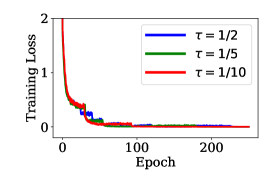
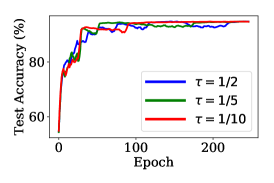
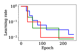
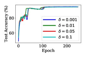
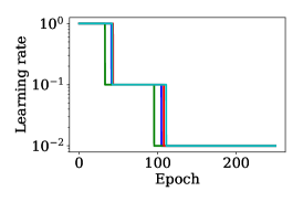
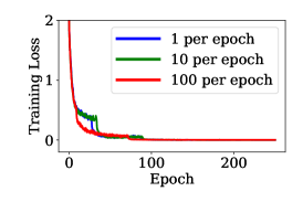
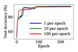
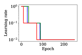
Figure 11: Sensitivity analysis of SASA+ on CIFAR10, using $\beta=0.9$ and $\nu=1$. The training loss, test accuracy, and learning rate schedule for SASA+ using different values of $\tau$ (first row), $\delta$ (second row), $\theta$ (third row), $K_{\textrm{test}}$ (fourth row on number of tests in an epoch) around the default values are shown, and the SASA+ applied on different methods (last row, i.e., SGD with momenton, NAG and QHM).

In the last row of Figure 11, we show that SASA+ can work with different optimization methods (i.e., SHB, NAG and QHM) on the CIFAR-10 dataset. Similar results for ImageNet are shown in Figure 12. We also show a sensitivity test of SASA+ on ImageNet with respect to $\tau$ (first row), $\delta$ (second row) and $\theta$ (third row) in Figure 13.

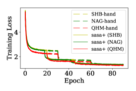
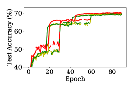
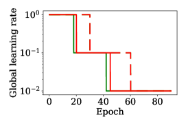
Figure 12: The dotted curves are stochastic optimization algorithms with hand-tuning learning rate, i.e., decrease every 30 epochs, as shown in the lower right panel. The solid curves are SASA+ combined with these 3 algorithms. SASA+ automatically adapts their learning rate (see the right panel) and achieves comparable and even slightly higher testing accuracy (see the middle panel).

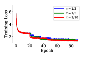
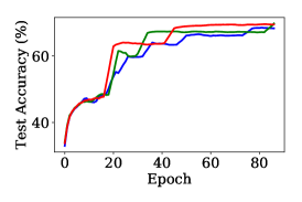
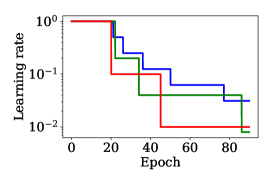
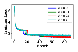
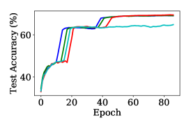
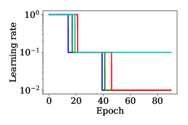
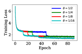
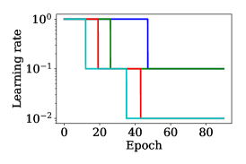
Figure 13: Sensitivity analysis of SASA+ on ImageNet, using $\beta=0.9$ and $\nu=1$. The training loss, test accuracy, and learning rate schedule for SASA+ using different values of $\tau$ (first row), $\delta$ (second row) and $\theta$ (third row) around the default values are shown.

In Figure 14, we show that the large LSTM model (as described in Section 4) quickly overfits the Wikitest-2 dataset, which can be seen from the quickly decreasing training loss but increasing validation perplexity for SASA and SASA+. Adding the validation dataset as another learning rate drop criterion avoids overfitting during training and to obtain good final performance on the validation/testing set.

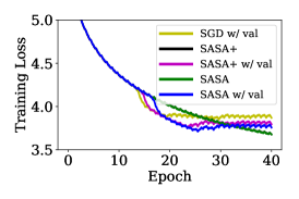
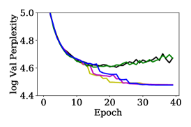
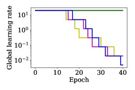
Figure 14: RNN: comparison of the baseline (SGD with validation dataset), SASA+ and SASA. The large LSTM model quickly overfits the Wikitest-2 dataset, which can be seen from the quickly decreasing training loss but increasing validation perplexity for SASA and SASA+. Adding the validation dataset as another learning rate drop criterion is necessary to avoid overfitting during training.

C.3 More results for SLOPE test

In addition to Figure 5, Figure 15 contains more results to comparing SASA+ and the SLOPE test. The learning rate schedules from SLOPE on CIFAR-10, ImageNet and MNIST are similar: it takes a few epochs for the first drop, and then the learning rate drops exponentially because the SLOPE test always fires (we do the test once every epoch). Due to the aggressive learning rate drop, the final testing performance is not comparable with SASA+ and hand-tuned SHB.

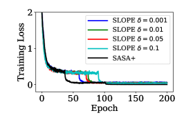
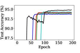
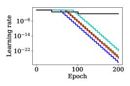
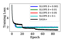
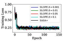
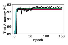
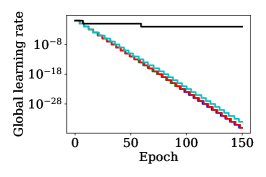
Figure 15: Comparison of SLOPE test and SASA+. SLOPE test is shown with the same default parameters as SASA+ and with different confidence levels $\delta$. First column: CIFAR-10 with ResNet18. Second column: ImageNet with ResNet18. Third column: MNIST with the linear model.

C.4 More results for SSLS

In Figure 6, we present the sensitivity analysis of SSLS on CIFAR-10. In Figure 16, 17 and 18, we show similar results on ImageNet, MNIST and Wikitest-2, respectively. These results confirm that:

• The final stable learning rate obtained by SSLS is robust to the initial learning rate $\alpha_{0}$. The dynamics starting from different initial learning rates are nearly the same.

• The final stable learning rate obtained by SSLS is robust to the smoothing factor $\gamma$. The smaller $\gamma$ is, the smoother the learning rate schedule is and the slower the process reaches the stable learning rate. Empirically, our recommended default $\gamma=\sqrt{b/n}$ achieves a good trade-off between smoothness of the learning rate schedule and the speed to reach the stable learning rate.

• The larger the sufficient decrease constant $c$ is, the smaller the final stable learning rate is. The final stable learning rates from different $c$’s are still at the same order, and are also at the same order of the hand-tuned initial learning rate.

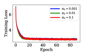
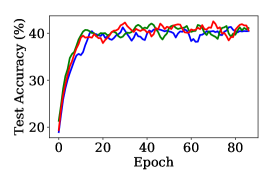
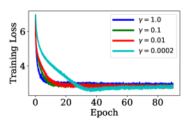
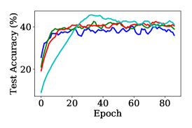
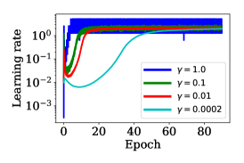
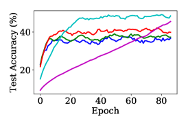
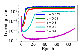
Figure 16: ImageNet: Sensitivity of SSLS to the initial learning rate $\alpha_{0}$ (first row), the smoothing factor $\gamma$ (second row) and the sufficient decrease constant $c$ (third row).

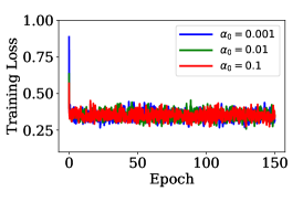
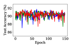
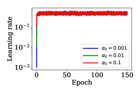
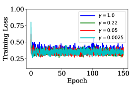
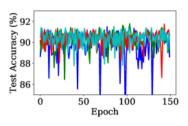
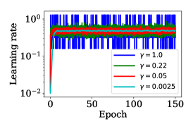
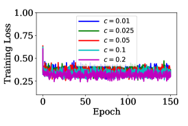
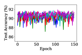
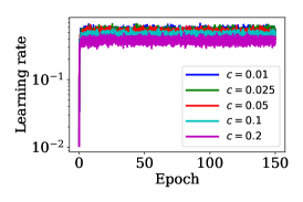
Figure 17: MNIST: Sensitivity of SSLS to the initial learning rate $\alpha_{0}$ (first row), the smoothing factor $\gamma$ (second row) and the sufficient decrease constant $c$ (third row).

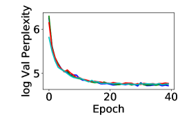
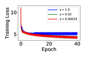
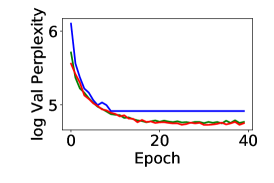
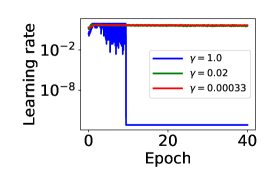
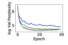
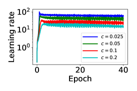
Figure 18: Wikitext-2: Sensitivity of SSLS to the initial learning rate $\alpha_{0}$ (first row), the smoothing factor $\gamma$ (second row) and the sufficient decrease constant $c$ (third row).

References

- Baydin et al. [2018] Atilim Günes Baydin, Robert Cornish, David Martínez Rubio, Mark Schmidt, and Frank Wood. Online learning rate adaptation with hypergradient descent. In Proceedings of the Sixth International Conference on Learning Representations (ICLR), Vancouver, Canada, 2018.
- Bottou [1998] Léon Bottou. Online algorithms and stochastic approximations. In David Saad, editor, Online Learning and Neural Networks. Cambridge University Press, Cambridge, UK, 1998. URL http://leon.bottou.org/papers/bottou-98x. Revised, Oct 2012.
- Delyon and Juditsky [1993] B. Delyon and A. Juditsky. Accelerated stochastic approximation. SIAM Journal on Optimization, 3(4):868–881, 1993.
- Deng et al. [2009] J. Deng, W. Dong, R. Socher, L.-J. Li, K. Li, and L. Fei-Fei. ImageNet: A Large-Scale Hierarchical Image Database. In CVPR09, 2009.
- Duchi et al. [2011] John Duchi, Elad Hazan, and Yoram Singer. Adaptive subgradient methods for online learning and stochastic optimization. Journal of Machine Learning Research, 12(Jul):2121–2159, 2011.
- Flegal and Jones [2010] James M Flegal and Galin L Jones. Batch means and spectral variance estimators in markov chain monte carlo. The Annals of Statistics, 38(2):1034–1070, 2010.
- Gitman et al. [2019] Igor Gitman, Hunter Lang, Pengchuan Zhang, and Lin Xiao. Understanding the role momentum in stochastic gradient methods. In Advances in Neural Information Processing Systems, volume 32, 2019.
- Goodfellow et al. [2016] Ian Goodfellow, Yoshua Bengio, and Aaron Courville. Deep Learning. MIT Press, 2016. http://www.deeplearningbook.org.
- Grimmett and Stirzaker [2001] Geoffrey Grimmett and David Stirzaker. Probability and Random Processes. Oxford University Press, 3rd edition, 2001.
- Gupal and Bazhenov [1972] A. M. Gupal and L. T. Bazhenov. A stochastic analog of the conjugate gradient method. Cybernetics, 8(1):138–140, 1972.
- He et al. [2016] Kaiming He, Xiangyu Zhang, Shaoqing Ren, and Jian Sun. Deep residual networks for image recognition. In Proceedgins of the 29th IEEE Conference on Computer Vision and Pattern Recognition (CVPR), pages 770–778, 2016.
- Jacobs [1988] R. A. Jacobs. Increased rates of convergence through learning rate adaption. Neural Networks, 1:295–307, 1988.
- Jain et al. [2018] Prateek Jain, Sham M Kakade, Rahul Kidambi, Praneeth Netrapalli, and Aaron Sidford. Accelerating stochastic gradient descent for least squares regression. In Conference On Learning Theory, pages 545–604, 2018.
- Jones et al. [2006] Galin L Jones, Murali Haran, Brian S Caffo, and Ronald Neath. Fixed-width output analysis for markov chain monte carlo. Journal of the American Statistical Association, 101(476):1537–1547, 2006.
- Kesten [1958] Harry Kesten. Accelerated stochastic approximation. Annals of Mathematical Statistics, 29(1):41–59, 1958.
- Kidambi et al. [2018] Rahul Kidambi, Praneeth Netrapalli, Prateek Jain, and Sham Kakade. On the insufficiency of existing momentum schemes for stochastic optimization. In 2018 Information Theory and Applications Workshop (ITA), pages 1–9. IEEE, 2018.
- Kingma and Ba [2014] Diederik P Kingma and Jimmy Ba. Adam: A method for stochastic optimization. arXiv preprint arXiv:1412.6980, 2014.
- Krizhevsky and Hinton [2009] Alex Krizhevsky and Geoffrey Hinton. Learning multiple layers of features from tiny images. Technical report, Citeseer, 2009.
- Lang et al. [2019] Hunter Lang, Pengchuan Zhang, and Lin Xiao. Using statistics to automate stochastic optimization. In Advances in Neural Information Processing Systems, volume 32, 2019.
- Lehmann and Romano [2005] Erich L. Lehmann and Joseph P. Romano. Testing Statistical Hypotheses. Springer, 3rd edition, 2005.
- Liu [2019] Kuang Liu. Pytorch cifar. Github repository, https://github.com/kuangliu/pytorch-cifar/tree/master/models, 2019.
- Ma and Yarats [2019] Jerry Ma and Denis Yarats. Quasi-hyperbolic momentum and adam for deep learning. In International Conference on Learning Representations, 2019.
- Mahmood et al. [2012] Ashique Rupam Mahmood, Richard S. Sutton, Thomas Degris, and Patrick M. Pilarski. Tuning-free step-size adaption. In Proceedings of the IEEE International Conference on Acoustics, Speech and Signal Processing (ICASSP), pages 2121–2124, 2012.
- Merity et al. [2016] Stephen Merity, Caiming Xiong, James Bradbury, and Richard Socher. Pointer sentinel mixture models. arXiv preprint arXiv:1609.07843, 2016.
- Mirzoakhmedov and Uryasev [1983] F. Mirzoakhmedov and S. P. Uryasev. Adaptive step adjustment for a stochastic optimization algorithm. Zh. Vychisl. Mat. Mat. Fiz., 23(6):1314–1325, 1983. [U.S.S.R. Comput. Math. Math. Phys. 23:6, 1983].
- Montgomery et al. [2012] D.C. Montgomery, E.A. Peck, and G.G. Vining. Introduction to Linear Regression Analysis. Wiley Series in Probability and Statistics. Wiley, 2012. ISBN 9780470542811. URL https://books.google.com/books?id=0yR4KUL4VDkC.
- Nesterov [2013] Y. Nesterov. Gradient methods for minimizing composite objective function. Mathematical Programming, Series B, 140:125–161, 2013.
- Nesterov [2004] Yurii Nesterov. Introductory Lecture on Convex Optimization: A Basic Course. Kluwer Academic Publishers, 2004.
- Nocedal and Wright [2006] Jorge Nocedal and Stephen J. Wright. Numerical Optimization. Springer, 2nd edition, 2006.
- Pflug [1983] Georg Ch. Pflug. On the determination of the step size in stochastic quasigradient methods. Collaborative Paper CP-83-025, International Institute for Applied Systems Analysis (IIASA), Laxenburg, Austria, 1983.
- Pflug [1988] Georg Ch. Pflug. Adaptive stepsize control in stochastic approximation algorithms. In Proceedings of 8th IFAC Symposium on Identification and System Parameter Estimation, pages 787–792, Beijing, 1988.
- Polyak [1964] Boris T. Polyak. Some methods of speeding up the convergence of iteration methods. USSR Computational Mathematics and Mathematical Physics, 4(5):1–17, 1964.
- Polyak [1977] Boris T. Polyak. Comparison of the rates of convergence of one-step and multi-step optimization algorithms in the presence of noise. Engineering Cybernetics, 15:6–10, 1977.
- Polyak and Juditsky [1992] Boris T Polyak and Anatoli B Juditsky. Acceleration of stochastic approximation by averaging. SIAM Journal on Control and Optimization, 30(4):838–855, 1992.
- PyTorch [2019] PyTorch. Pytorch word language model. https://github.com/pytorch/examples/tree/master/word_language_model, 2019.
- Robbins and Monro [1951] Herbert Robbins and Sutton Monro. A stochastic approximation method. The Annals of Mathematical Statistics, 22(3):400–407, 1951.
- Ruszczyński and Syski [1983] Andrzej Ruszczyński and Wojciech Syski. Stochastic approximation method with gradient averaging for unconstrained problems. IEEE Transactions on Automatic Control, 28(12):1097–1105, 1983.
- Ruszczyński and Syski [1984] Andrzej Ruszczyński and Wojciech Syski. Stochastic approximation algorithm with gradient averaging and on-line stepsize rules. In J. Gertler and L. Keviczky, editors, Proceedings of 9th IFAC World Congress, pages 1023–1027, Budapest, Hungary, 1984.
- Ruszczyński and Syski [1986a] Andrzej Ruszczyński and Wojciech Syski. On convergence of the stochastic subgradient method with on-line stepsize rules. Journal of Mathematical Analysis and Applications, 114:512–527, 1986a.
- Ruszczyński and Syski [1986b] Andrzej Ruszczyński and Wojciech Syski. A method of aggregate stochastic subgradients with on-line stepsize rules for convex stochastic programming problems. Mathematical Programming Study, 28:113–131, 1986b.
- Schmidt et al. [2017] Mark Schmidt, Nicolas Le Roux, and Francis Bach. Minimizing finite sums with the stochastic average gradient. Mathematical Programming, 162(1-2):83–112, 2017.
- Schraudolph [1999] Nicol N. Schraudolph. Local gain adaptation in stochastic gradient descent. In Proceedings of Nineth International Conference on Artificial Neural Networks (ICANN), pages 569–574, 1999.
- Streiner [2003] David L Streiner. Unicorns do exist: A tutorial on “proving” the null hypothesis. The Canadian Journal of Psychiatry, 48(11):756–761, 2003.
- Sutskever et al. [2013] Ilya Sutskever, James Martens, George Dahl, and Geoffrey Hinton. On the importance of initialization and momentum in deep learning. In Sanjoy Dasgupta and David McAllester, editors, Proceedings of the 30th International Conference on Machine Learning, volume 28 of Proceedings of Machine Learning Research, pages 1139–1147, Atlanta, Georgia, USA, 17–19 Jun 2013. PMLR.
- Sutton [1992] Richard S. Sutton. Adapting bias by gradient descent: An incremental version of Delta-Bar-Delta. In Proceedings of the Tenth National Conference on Artificial Intelligence (AAAI’92), pages 171–176. The MIT Press, 1992.
- Tieleman and Hinton [2012] Tijmen Tieleman and Geoffrey Hinton. Lecture 6.5-rmsprop: Divide the gradient by a running average of its recent magnitude. COURSERA: Neural networks for machine learning, 4(2):26–31, 2012.
- Vaswani et al. [2019] Sharan Vaswani, Aaron Mishkin, Issam Laradji, Mark Schmidt, Gauthier Gidel, and Simon Lacoste-Julian. Painless stochastic gradient: Interpolation, line-search, and convergence rates. In Advances in Neural Information Processing Systems, volume 32, 2019.
- Wilson et al. [2017] Ashia C Wilson, Rebecca Roelofs, Mitchell Stern, Nati Srebro, and Benjamin Recht. The marginal value of adaptive gradient methods in machine learning. In Advances in Neural Information Processing Systems, pages 4148–4158, 2017.
- Yaida [2018] Sho Yaida. Fluctuation-dissipation relations for stochastic gradient descent. arXiv preprint arXiv:1810.00004, 2018.