The Hills Mechanism and the Galactic Center S-stars

Abstract

Our Galactic center contains young stars, including the few million year old clockwise disk between 0.05 and 0.5 pc from the Galactic center, and the S-star cluster of B-type stars at a galactocentric distance of $\sim$0.01 pc. Recent observations suggest the S-stars are remnants of tidally disrupted binaries from the clockwise disk. In particular, Koposov et al. (2020) discovered a hypervelocity star that was ejected from the Galactic center 5 Myr ago, with a velocity vector consistent with the disk. We perform a detailed study of this binary disruption scenario. First, we quantify the plausible range of binary semimajor axes in the disk. Dynamical evaporation of such binaries is dominated by other disk stars rather than by the isotropic stellar population. For the expected range of semimajor axes in the disk, binary tidal disruptions can reproduce the observed S-star semimajor axis distribution. Reproducing the observed thermal eccentricity distribution of the S-stars requires an additional relaxation process. The flight time of the Koposov star suggests that this process must be effective within 10 Myr. We consider three possibilities: (i) scalar resonant relaxation from the observed isotropic star cluster, (ii) torques from the clockwise disk, and (iii) an intermediate-mass black hole. We conclude that the first and third mechanisms are fast enough to reproduce the observed S-star eccentricity distribution. Finally, we show that the primary star from an unequal-mass binary would be deposited at larger semimajor axes than the secondary, possibly explaining the dearth of O stars among the S-stars.

1 Introduction

The Galactic center contains a population of young stars. This population includes a disk of O, B, and Wolf–Rayet stars between 0.05 and 0.5 pc from the center (the clockwise disk; Levin & Beloborodov 2003; Paumard et al. 2006) as well as an isotropic cluster of B stars at $\sim 0.01$ pc (the S-stars; Gillessen et al. 2017). The presence of young stars on these scales is a challenge for current theories of star formation, as strong tidal forces would shred molecular clouds at the present location of the clockwise disk (Ghez et al., 2003). One proposed solution is that the disk stars formed from a Toomre unstable gas accretion disk (Levin, 2007). However, it is unlikely that this instability could extend to the present-day location of the S-stars (in particular, to the present-day orbit of S2; Nayakshin & Cuadra 2005).

Instead, the S-stars may have migrated from larger scales, either via interactions with a gas disk (Levin, 2007), or via the Hills mechanism (Hills, 1988; Ginsburg & Loeb, 2006; Perets et al., 2007; Löckmann et al., 2009; Madigan et al., 2009; Dremova et al., 2019). In the latter case, binaries are scattered close to the central supermassive black hole (SMBH) and tidally disrupted. One of the stars in the binary escapes at high velocity, while the other remains bound to the central SMBH. The bound stars can steepen the stellar density profile in the Galactic center and enhance the rate of stellar tidal disruption events and extreme mass ratio inspirals (Fragione & Sari, 2018; Sari & Fragione, 2019). Binaries may originate from large ($\mathrel{\hbox to0.0pt{\lower 4.0pt\hbox{\hskip 1.0pt$\sim$}\hss}\raise 1.0pt\hbox{$>$}}$ pc) scales (Perets et al., 2007), disruption of a young star cluster (Fragione et al., 2017), or from the clockwise disk itself (Madigan et al., 2009). The latter scenario is particularly attractive, as recent observations indicate that the age of the S-stars is consistent with the age of the clockwise disk (Habibi et al., 2017). Furthermore, a recently discovered hypervelocity star also points to a disk origin for the S-stars (Koposov et al., 2020). This star is noteworthy because, of all of the known hypervelocity stars, it has the strongest case for a Galactic center origin (see Figure 5 of Koposov et al. 2020). This star has a velocity vector consistent with the clockwise disk. Also, the flight time of this star from the Galactic center (4.8 Myr) is comparable to the disk’s age. While the evidence for a disk origin for this star is not quite definitive, the most parsimonious explanation for these observations is that some binaries from the disk underwent disruptions a few million years ago, which would have left a population similar to the observed S-stars.

Other models for the origins of the S-stars include compression and fragmentation of an outflowing spherical shell (Nayakshin & Zubovas, 2018) and scattering of binaries by stellar mass black holes (Trani et al., 2019). However, neither of these models would account for the observed hypervelocity star.

Within the Hills scenario, it is difficult to reproduce the observed thermal eccentricity distribution of the S-stars (Gillessen et al., 2017). The Hills mechanism would place stars on highly eccentric orbits (e.g. Antonini & Merritt 2013). Thus, a subsequent relaxation process must be invoked to reproduce the observations.

In this paper, we revisit the viability of the Hills mechanism as a source of the S-stars. Motivated by the similar ages of the disk and S-stars, we focus on the case where the source binaries originate in the clockwise disk as in Madigan et al. 2009. First, we quantify the plausible range of binary parameters within this disk, including the effects of dynamical evaporation. We find that the disk stars dominate this process, even though they are less numerous than the old, isotropic population in the Galactic center. We then simulate a large ensemble of close encounters between disk binaries and the central SMBH. Remnants from these encounters can account for the semimajor axis distribution of the S-stars, but their eccentricities are too high.

We consider three possible mechanisms that could reproduce the observed S-star eccentricities: (i) scalar resonant relaxation (SRR) due to the surrounding isotropic cluster, (ii) torques from the clockwise disk and (iii) an intermediate-mass black hole (IMBH) near the S-stars. SRR occurs in highly symmetric potential where long-term correlations between stellar orbits lead to a build–up of coherent torques that change the stars’ eccentricity (Rauch & Tremaine, 1996). Previous works (e.g. Antonini & Merritt 2013) find that the SRR timescale near the S-stars can be as short as $\sim 10^{7}$ years if the effects of stellar mass black holes are included. Here we revisit this estimate in light of new theoretical developments in the theory of resonant relaxation. Specifically, we use the formalism of Bar-Or & Fouvry (2018), who derived diffusion coefficients for resonant relaxation from the orbit-averaged Hamiltonian of a star in a spherically symmetric star cluster. In agreement with Antonini & Merritt (2013), we find that a realistic population of stellar mass black holes can reproduce the eccentricity distribution of the S-stars within $10^{7}$ years. This timescale is comparable to the ages of the S-stars and flight time of the Koposov et al. (2020) star. We find that torques from the clockwise disk are quenched by general relativistic precession and would not be able to reproduce the S-stars’ eccentricity distribution. Previously, IMBHs have been considered as a mechanism for reproducing the orbital properties of the S-stars (Merritt et al., 2009), though this work did not consider stars on highly eccentric orbits as would be expected from the Hills mechanism. Here we show that an $\sim 10^{3}M_{\odot}$ IMBH at $\sim$0.01 pc thermalizes the S-star orbits within a few Myr, starting from an initial eccentricity that is $\mathrel{\hbox to0.0pt{\lower 4.0pt\hbox{\hskip 1.0pt$\sim$}\hss}\raise 1.0pt\hbox{$>$}}$0.97.

The remainder of this paper is organized as follows. We review the disk instability that pushes binaries to tidal disruption in $\S$ 2. In $\S$ 3 we discuss the plausible range of binary properties within the clockwise disk. We then simulate a large number of close encounters between disk binaries and the Galactic center SMBH, as summarized in $\S$ 4 and $\S$ 5. We explore various processes that could reproduce the observed S-star eccentricity distribution in $\S$ 6. Finally, we consider other consequences of tidal encounters between binaries and SMBHs in $\S$ 7.

2 Eccentric disk instability

If the clockwise disk started as a high-eccentricity ($e\mathrel{\hbox to0.0pt{\lower 4.0pt\hbox{\hskip 1.0pt$\sim$}\hss}\raise 1.0pt\hbox{$>$}}0.6$), lopsided structure, some of its stars and binaries could have been excited to nearly radial orbits and tidally disrupted as described in Madigan et al. (2009). Briefly, stars in the disk precess retrograde to their orbital angular momenta due to the influence of the surrounding star cluster (Madigan et al., 2011; Merritt, 2013). Stars with higher eccentricities precess more slowly and end up behind the bulk of the disk, which then torques them to even higher eccentricities. Eventually, such stars (or binaries) may be tidally disrupted. Bonnell & Rice (2008) and Mapelli et al. (2012) found that such a lopsided, eccentric disk could arise from the disruption of a molecular cloud in the Galactic center (see, e.g. Figure 2 in the latter).

To illustrate the development of this instability, we perform N-body simulations of an eccentric, apsidally aligned disk, closely following Madigan et al. (2009) for our initial conditions. Specifically, we initialize a disk with 100 point masses of $100\,M_{\odot}$ each (for a total disk mass of $10^{4}M_{\odot}$), orbiting a $4\times 10^{6}\,M_{\odot}$ SMBH. The disk stars have semimajor axes between 0.05 pc and 0.5 pc with an $r^{-2}$ surface density profile like the clockwise disk. All stars start with an initial eccentricity of 0.7 and nearly aligned eccentricity and angular momentum vectors. The simulations also include the potential of an $r^{-1.5}$ stellar density profile, with $4\times 10^{6}M_{\odot}$ of stars within 4 pc.

We integrate the disk forward in time with the IAS15 integrator of the REBOUND N-body code (Rein & Liu, 2012; Rein & Spiegel, 2015). We also include an approximate treatment of general relativity (GR) effects via REBOUNDX (Tamayo et al., 2020). Any particles that pass within $3\times 10^{-4}$ pc of the central SMBH are recorded as binary disruptions. In general, these stars are not removed from the simulation to keep the disk potential as constant as possible, but we only record one disruption per particle.

The top panel of Fig. 1 shows the initial orbits of disk stars for a particular simulation, while the bottom panel shows the disk orbits after $\sim 4$ Myr. By this time, the orbits are spread out and have a bimodal eccentricity distribution, as shown in Fig. 2 (see also Madigan et al. 2009; Gualandris et al. 2012). Bartko et al. (2009) claimed detection of a bimodal eccentricity distribution within the clockwise disk. However, subsequent work has argued that these measurements are contaminated by nondisk stars and favor a unimodal eccentricity distribution with a mean eccentricity of $0.27\pm 0.07$ (Yelda et al., 2014). The latter observation would disfavor the eccentric disk scenario. However, caution is warranted in interpreting these observations, as disk membership and the observed disk eccentricities may be contaminated by binary stars (Naoz et al., 2018).

Only a few percent of the particles in our simulations undergo disruptions compared to $\sim 30$ percent for simulations with similar initial conditions in Madigan et al. (2009). However, the total number of disruptions is sensitive to the slope of the stellar density profile, and the total mass of the disk. In particular, the disk may have been more massive earlier in its history, when gas was still present. Doubling the mass of the disk to $\sim 2\times 10^{4}M_{\odot}$, and taking a flatter $r^{-1.1}$ stellar density profile (motivated by Schödel et al. 2018), increases the disrupted fraction up to 17 $\pm$ 2 percent.

Fig. 3 shows binary disruptions occur promptly after the disk forms. In particular, disruptions begin at a few times the disk’s secular time, viz.

$$t_{\rm sec}=\frac{M}{M_{d}}P,$$ (1)

where $M$ and $M_{d}$ are the SMBH and disk mass respectively, and $P$ is the orbital period. Here $t_{\rm sec}\approx 1-2\times 10^{5}$ years at 0.05 pc (the inner edge of the clockwise disk).

We note that although our simulations have approximately an order of magnitude fewer stars than the real disk, Madigan et al. (2018) found that the number of disruptions in eccentric disk simulations depends weakly on the number of particles. This is expected, because the secular torques from the disk would not depend on the number of stars it contains. We have also run some simulations with 300 particles for 1.4 Myr and find a similar disrupted fraction. For example, we find a disrupted fraction of 14 $\pm$ 1% (17 $\pm$ 2%) for 300 (100) particle simulations with an $r^{-1.1}$ stellar background and a $2\times 10^{4}M_{\odot}$ disk.

Overall, these simulations show that an eccentric, apsidally aligned disk can produce a large number of binary disruptions via a secular instability. In particular, these simulations show the clockwise can reproduce the observed number of S-stars (see $\S$ 5.2) soon after its formation.

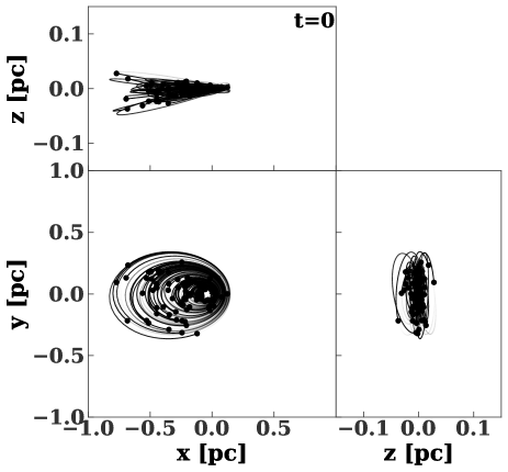
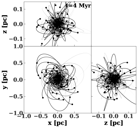
Figure 1: Top panel: initial orbits for an N-body simulation of an eccentric, apsidally aligned disk in the Galactic center. Bottom panel: The disk after 4 Myr of evolution, after the eccentric disk instability has developed.

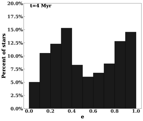
Figure 2: Bimodal eccentricity distribution of an evolved, eccentric disk in the Galactic center. This distribution is constructed by stacking the results of four different simulations (like the one shown in Fig. 1). The initial eccentricity distribution is a delta function at $e=0.7$.

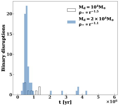
Figure 3: Times when binaries are disrupted in our disk simulations ($t=0$ is the start of the simulation). The blue filled histogram shows the distribution of disruption times for simulations with a $2\times 10^{4}M_{\odot}$ disk and an $r^{-1.1}$ background stellar density profile, while the black open histogram shows the distribution of disruption times for simulations with a $10^{4}M_{\odot}$ disk and a $r^{-1.5}$ stellar background. Binary disruptions begin after a secular time ($1-2\times 10^{5}$ years). Each distribution is constructed by stacking the results of four different simulations.

2.1 Full or empty loss cone?

In order to be tidally disrupted, a binary has to enter into a loss cone of low angular momentum orbits that pierce the tidal radius. Binaries can be in either the empty or full loss cone regime. In the former case, binaries would diffuse into the loss cone over many orbital periods. In the latter case, binaries can jump into and out of the loss cone in a single orbital period. Here we show that disk binaries are in the empty loss cone regime.

The typical torque per unit mass from the disk is

$$\tau_{d}\sim\frac{GM_{d}}{a_{d}},$$ (2)

where $M_{\rm d}\approx 10^{4}M_{\odot}$ is the disk mass and $a_{d}$ is a characteristic semimajor axis for a disk orbit. The change in angular momentum per orbit due to this torque is

$$\Delta j=\tau_{d}P(a_{d})\equiv Qj_{\rm lc}\implies$$

$$Q=\frac{2\pi}{\sqrt{2}}\frac{M_{\rm disk}}{M}\sqrt{\frac{a_{d}}{r_{t}}}$$

$$Q\approx 0.27\left(\frac{a_{\rm bin}}{1\,{\rm au}}\right)^{-1/2}\left(\frac{a_{d}}{0.1\,{\rm pc}}\right)^{1/2}\left(\frac{m}{20\,M_{\odot}}\right)^{1/6}$$ (3)

where $P(a_{d})$ is the orbital period and $j_{\rm lc}$ is the loss cone angular momentum (see also Wernke & Madigan 2019 equation 12). Thus, disk binaries are typically in the empty loss cone regime ($Q<1$), and approach the tidal radius gradually over several orbits.

3 Galactic center Binary Population

An SMBH can tidally disrupt a binary into two stars. The postdisruption orbits of these stars depend on the initial properties (e.g. the semimajor axis and eccentricity) of the binary. In this section, we quantify the plausible range of binary properties of the young stellar population in the clockwise disk in the Galactic center.

3.1 Binary dynamics

Binaries with a semimajor axis

$$a_{\rm bin}>a_{\rm hs}=\frac{Gm_{1}m_{2}}{\sigma^{2}<m>},$$

are soft and will evaporate over time. Here $m_{1}$ and $m_{2}$ are the masses of the primary and secondary star in the binary, respectively; $<m>$ and $\sigma$ are the mean mass and the velocity dispersion of the surrounding stellar population. The timescale for evaporation is

$$t_{\rm evap}=0.07\frac{v_{12}^{2}\sigma}{G^{2}n<m^{2}>\ln\Lambda_{12}},$$ (5)

where $v_{12}$ is the (internal) orbital velocity of the binary, $<m^{2}>$ is the second moment of the stellar mass function, $n$ is the stellar number density, and $\Lambda_{12}\approx 2\sigma^{2}/v_{12}^{2}$ (see equation 3 of Alexander & Pfuhl 2014). From Equation (5), soft binaries at a galactocentric radius $r$ with

$$a_{\rm bin}>a_{\rm evap}=e^{W(t_{a}/t)}\frac{Gm}{2\sigma^{2}}$$ (6)

$$t_{a}=\frac{0.14\sigma^{3}}{G^{2}n<m^{2}>},$$ (7)

would have evaporated after time $t$. Here $m$ is the total mass of the binary and $W$ is the Lambert $W$ function.

Gravitational wave emission and finite stellar radii set a lower limit on the binary semi-major axis. Within time $t$, binaries with

$$a_{\rm bin}<a_{\rm GW}=\left[\frac{5c^{5}}{256G^{3}m^{3}t}\frac{(1+q)^{2}}{q}f(e_{\rm bin})\right]^{-1/4}$$ (8)

$$f(e)=\frac{(1-e^{2})^{7/2}}{1+\frac{73}{24}e^{2}+\frac{37}{96}e^{4}}$$ (9)

would have coalesced. Here $e$ and $q$ are the binary eccentricity and mass ratio (see Peters 1964 equation 5.6). Binaries with

$$a_{\rm bin}(1-e_{\rm bin})<a_{\rm Roche}$$

$$={\rm max}[R_{1}/h(m_{1}/m_{2}),R_{2}/h(m_{2}/m_{1})]$$

$$h(q)=\frac{0.49q^{2/3}}{0.6q^{2/3}+\log(1+q^{1/3})},$$ (10)

will experience Roche lobe overflow (Eggleton, 1983). Here $m_{1}$ and $m_{2}$ are the masses of the individual stars, and $R_{1}$ and $R_{2}$ are their radii. We consider $a_{\rm roche}$ to be a lower limit to the binary separation. For the young stars in the clockwise disk, $a_{\rm GW}<a_{\rm Roche}$, and gravitational wave inspiral is unimportant.

Kozai–Lidov oscillations can also be important for binaries in the Galactic center (Lidov, 1962; Kozai, 1962; Antonini & Perets, 2012; Prodan et al., 2015; Stephan et al., 2016; Fragione & Antonini, 2019). The quadrupole Kozai–Lidov timescale at the inner edge of the clockwise disk is

$$t_{\rm KL}=2.1\times 10^{5}{\rm yr}\left(\frac{m}{20M_{\odot}}\right)^{1/2}\left(\frac{a_{\rm bin}}{1{\rm au}}\right)^{-3/2}.$$ (11)

The octupole Kozai–Lidov timescale is (see the review by Naoz 2016)

$$t_{\rm KL,oct} \approx\frac{t_{\rm KL}}{\epsilon}$$

$$=\frac{a_{d}}{a_{\rm bin}}\frac{1-e_{d}^{2}}{e_{d}}t_{\rm KL}$$

$$\approx 10^{4}\left(\frac{a_{\rm bin}}{1{\rm au}}\right)^{-1}\frac{1-e_{d}^{2}}{e_{d}}t_{\rm KL},$$ (12)

where the subscript “d” denotes properties of the disk binaries’ outer orbits, and in the third line we take $a_{d}=0.05$ pc. Thus, $t_{\rm KL,oct}$ is typically $\mathrel{\hbox to0.0pt{\lower 4.0pt\hbox{\hskip 1.0pt$\sim$}\hss}\raise 1.0pt\hbox{$>$}}10^{9}$ years, and octupole level effects can be neglected for the few million years old disk stars. Therefore, Kozai–Lidov oscillations would only occur for highly inclined, wide binaries ($a_{\rm bin}\mathrel{\hbox to0.0pt{\lower 4.0pt\hbox{\hskip 1.0pt$\sim$}\hss}\raise 1.0pt\hbox{$>$}}1$ AU) for which the precession timescale due to GR is longer than the Kozai–Lidov timescale. We expect the disk binaries to have low inclinations (i.e. their internal angular momentum is aligned with the angular momentum of their outer orbit around the SMBH). Vector resonant relaxation may realign the outer orbits of binaries in the disk on $\sim$Myr timescales (Kocsis & Tremaine, 2011). Nonetheless, the eccentric disk instability is also quite fast and can produce binary disruptions on a similar timescale (see Fig. 3). Moreover, the binaries that are disrupted would be precisely those with small inclinations, as secular torques from the disk would be aligned with their angular momentum vectors (Madigan et al., 2018; Foote et al., 2020).

3.2 The Galactic center

There are two populations that can perturb binaries in the $\sim 4$ Myr old (Lu et al., 2013) clockwise disk: (1) the surrounding old, isotropic star cluster and (2) the disk stars themselves.

To see which is more important, we compare the evaporation timescales of the two populations (Equation 5). The disk stars will have a shorter evaporation timescale and will dominate evaporation if

$$\frac{n_{\rm iso}<m^{2}>_{\rm iso}}{\sigma_{\rm iso}}\leq\frac{n_{d}<m^{2}>_{d}}{\sigma_{d}},$$ (13)

where subscripts “$d$” and “${\rm iso}$” indicate the disk and isotropic populations respectively. Note that $\sigma_{d}/\sigma_{\rm iso}\approx(H/r)$, where $H$ is the scale height of the disk.

There are $\sim$1000 stars in the disk with an $r^{-2}$ surface density profile between $\sim$0.05 and $\sim$0.5 pc (Paumard et al., 2006; Do et al., 2013). Thus,

$$n_{\rm d}\sim 6.3\times 10^{4}\left(\frac{H}{r}\right)^{-1}\left(\frac{r}{0.1{\rm pc}}\right)^{-3}{\rm pc}^{-3}.$$ (14)

For the observed $M^{-1.7}$ (Lu et al., 2013) mass function in the disk

$$<m^{2}>_{d}^{1/2}\approx 11M_{\odot}.$$ (15)

We assume that this mass function extends from 1 $M_{\odot}$ to 60 $M_{\odot}$ (the main sequence turn-off mass for a 4 Myr old stellar population).

The stellar density in the isotropic component can be constrained by existing observations. For example, Schödel et al. (2018) found that the stellar density is $\sim 1-2\times 10^{5}M_{\odot}$ pc^-3 one parsec from the Galactic Center with an $r^{-1.13\pm 0.03_{\rm model}\pm 0.05_{\rm sys}}$ profile. However, the mean square mass will be a strong function of the number of stellar mass black holes in the isotropic component. We adopt the Fiducial$\times 10$ model from Generozov et al. (2018) for the black hole density profile. The black holes in this model are formed near the present day clockwise disk. The present epoch is assumed to be typical, so $\sim$300 massive stars form every few million years, and become black holes and neutron stars. This model approximately reproduces the observed stellar density profile in the Galactic center, as well as the recently discovered population of black hole X-ray binaries in the central parsec (Hailey et al., 2018; Mori et al., 2019) via tidal capture of main-sequence stars. This model implicitly assumes that the initial mass function in the disk is truncated near $10M_{\odot}$, which is problematic, as the hypervelocity star observed by Koposov et al. (2020) is an A-type star with a few solar masses. Nonetheless, the black hole density profile in the Fiducial$\times 10$ model is within a factor of a few of previous estimates on the scales of interest, which assume that black holes and low-mass stars form as a single population with a standard mass function (see the review by Alexander et al. 2017 and the references therein).

In the Fiducial$\times 10$ model

$$n_{\rm iso}\approx 5\times 10^{6}\left(\frac{r}{0.1\,\,{\rm pc}}\right)^{-1.5}{\rm pc}^{-3}$$ (16)

and

$$<m^{2}>_{\rm iso}^{1/2}\approx 7\left(\frac{r}{0.1{\rm pc}}\right)^{-0.3}M_{\odot}$$ (17)

between $0.01$ pc and $0.1$ pc. The number density is dominated by main sequence stars, but stellar mass black holes dominate the two–body relaxation on these scales. From equations (13) the disk stars dominate the evaporation of binaries for disk aspect ratios

$$\frac{H}{r}\lesssim 0.18\left(\frac{r}{0.1\,{\rm pc}}\right)^{-0.45}.$$ (18)

This inequality should be satisfied in the clockwise disk, which has an observed $H/r\approx 0.1$ (Paumard et al., 2006).

4 Binary disruption ensemble

We simulate an ensemble of encounters between stellar binaries and a $4\times 10^{6}{\rm M_{\odot}}$ SMBH, where the binaries pass near their tidal radius. The binary properties in this ensemble are summarized in Table 1.

Table 1: Summary of Parameters for our Monte Carlo Simulations of Binary–SMBH Encounters.

Parameter	Distribution	Lower Bound	Upper Bound
$a_{\rm bin}$	$a_{\rm bin}^{-1}$	Equation 19	Equation 20
$m_{1}$	$m_{1}^{-1.7}$	$8M_{\odot}$	$15M_{\odot}$
$e$	0, thermal	0	1

Note. — The three rows are the binary semimajor axis, the mass of each star, and the eccentricity. The mass ratio is unity and the pericenter is the effective tidal radius (Equation 22).

We draw the binary semimajor axis from a log-uniform distribution. The maximum semimajor axis is set by dynamical evaporation, while the minimum semimajor axis is set by finite stellar radii and gravitational wave emission. In particular, the semimajor axis distribution extends from

$$a_{\rm min}={\rm max}\left[a_{\rm gw},a_{\rm roche}\right]$$ (19)

to

$$a_{\rm max}={\rm min}\left[{\rm max}\left[a_{\rm hs},a_{\rm evap}\right],100{\,\rm au}\right].$$ (20)

The semimajor axes on the right-hand side of the above equations are defined in $\S$ 3.1 (see equations LABEL:eq:ahs, 7, 9, and 10). These quantities are functions of the binary mass, mass ratio, and eccentricity. They also depend on the galactocentric radius and the age of the binaries. We evaluate $a_{\rm min}$ and $a_{\rm max}$ assuming 4 Myr old stars at a galactocentric radius of 0.1 pc. Note we use the disk properties (number density, velocity dispersion, and mean square mass) to evaluate $a_{\rm hs}$ and $a_{\rm evap}$. In particular, we use equations (14) and (15) for the number density and mean squared mass respectively. The velocity dispersion is $\sqrt{GM/r}(H/r)$, $H/r$ is the disk aspect ratio (0.1 here).

Fig. 4 shows the minimum and maximum semimajor axes as function of binary mass for two different binary eccentricities.

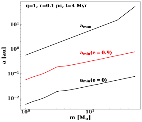
Figure 4: Minimum and maximum possible semi-major axis as a function of mass for binaries within the clockwise disk at a galactocentric distance of 0.1 pc. The stars in the binary have equal masses ($q=1$).

The stellar masses are drawn from the observed mass function of the disk (Lu et al., 2013). As the observed S-stars are all B–stars we consider only stars between 8 and 15 $M_{\odot}$ (these are approximately minimum and maximum masses of the eight S-stars studied by Habibi et al. 2017). The mass ratio of the binary is taken to be one for simplicity. We use two different distributions for the internal binary eccentricity (circular and thermal).

As noted in § 2.1, binary disruptions will likely be in the empty loss cone regime. In this regime, the pericenter distribution of tidally disrupting single stars is strongly peaked at the tidal radius. The binary case is more complicated, as the disruption probability gradually increases as the pericenter decreases.

The top panel of Fig. 5 shows the probability for a binary to disrupt as a function of its pericenter and its internal eccentricity. For any combination of these parameters, the outcome of a close encounter between a binary and an SMBH is determined by the binary’s phase. The disruption probability first becomes nonzero between $\sim 2$ and $3r_{t,o}$, where

$$r_{t,o} \equiv\left(\frac{M}{m_{\rm bin}}\right)^{1/3}a_{\rm bin}$$

$$=2.8\times 10^{-4}\left(\frac{m_{\rm bin}}{20M_{\odot}}\right)^{-1/3}\left(\frac{a_{\rm bin}}{1\,\,\rm au}\right){\rm\,\,pc}.$$ (21)

The probabilistic nature of binary disruptions implies that there would be a spread in the pericenters of disrupting binaries even in the empty loss cone regime. Here we do not attempt to model this distribution but assume that all binaries are disrupted at an effective tidal radius

$$r_{t}\equiv\chi r_{t,o}=\chi\left(\frac{M}{m_{\rm bin}}\right)^{1/3}a_{\rm bin}.$$ (22)

The prefactor $\chi$ is a function of the internal binary eccentricity. We define $\chi$ so that a binaries have a 50% disruption probability at the effective tidal radius. The bottom panel of Fig. 5 shows $\chi$ as a function of the binary eccentricity.

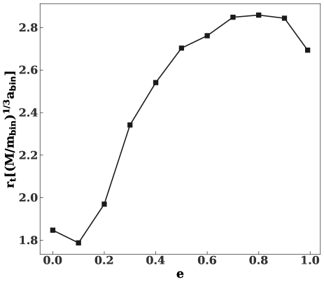
Figure 5: Top panel: probability of binary disruption as a function of the binary pericenter and internal eccentricity. Binary disruption is probabilistic as it depends on the phase of the binary. This calculation assumes the binary’s center-of-mass orbit is parabolic. Bottom panel: effective tidal radius as a function of binary eccentricity (see Equation 22 and the surrounding discussion).

4.1 Method

We solve for the positions of the stars using both the parabolic Hills approximation (Sari et al., 2010) as well as direct three-body integration with AR--Chain (Mikkola & Merritt, 2008). In both cases post-Newtonian effects are neglected (Antonini et al. 2010 conclude that the latter would be negligible except for the closest binaries). The binary’s center of mass orbit is approximated as parabolic unless otherwise noted.

The presented results in the main text are from AR--Chain integrations. However, we find that the Hills approximation is generally accurate, as discussed in Appendix A.

5 Results

5.1 Distributions of orbital elements

Taylor expanding the potential energy about the tidal radius gives the spread in orbital energy across the binary when it is disrupted, viz.

$$\Delta E=k^{\prime}\frac{GMm_{\rm bin}a_{\rm bin}q}{r_{t}^{2}(1+q)^{2}},$$ (23)

where $q$, $m_{\rm bin}$, and $a_{\rm bin}$ are the mass ratio of the secondary to the primary, total mass, and semimajor axis of the binary and $k^{\prime}$ is a factor of order unity (Hills, 1988; Yu & Tremaine, 2003). After the disruption, one of the stars is left on a bound orbit with energy

$$E_{s}=\frac{GMm_{s}}{2a_{s}},$$ (24)

where $m_{s}$ is the mass of the star, and $a_{s}$ is its postdisruption semimajor axis. For a parabolic disruption, $E_{s}=\Delta E$. Therefore,

$$a_{s} =\underbrace{\frac{\chi^{2}}{k^{\prime}}}_{1/k}\frac{m_{s}}{m_{\rm bin}}\frac{(1+q)^{2}}{2q}\left(M/m_{\rm bin}\right)^{2/3}a_{\rm bin}$$

$$=\frac{1}{k}\left(M/m_{\rm bin}\right)^{2/3}a_{\rm bin}$$

$$\approx 0.016\left(\frac{m_{\rm bin}}{20M_{\odot}}\right)^{-2/3}\left(\frac{a_{\rm bin}}{1\,{\rm au}}\right){\rm pc},$$ (25)

where $k\approx 0.3-1$ depends on the phase and eccentricity of the binary. In the second line of Equation (25), we assume the binary stars are equal in mass.

The bound star will have approximately the same pericenter as the original binary orbit. Therefore, its eccentricity is

$$e_{s}\approx 1-\chi k\left(\frac{M}{m_{\rm bin}}\right)^{-1/3},$$ (26)

where $\chi k\approx 1-2$. Fig. 6 shows the postdisruption semimajor axis and eccentricity distributions for the bound stars in our ensemble of simulated binary–SMBH encounters. As expected, the bound stars are on highly eccentric orbits ($e\mathrel{\hbox to0.0pt{\lower 4.0pt\hbox{\hskip 1.0pt$\sim$}\hss}\raise 1.0pt\hbox{$>$}}0.96$) with semimajor axes between $\sim 10^{-3}$ and $1$ pc. For thermal eccentricity binaries, the semimajor axis distribution of remnant stars inside the inner edge of the disk ($\sim$ 0.05 pc) is statistically consistent with the semimajor axis distribution of S-stars in this region.The two distributions are not statistically consistent in the case of circular binaries. However, this can be fixed by taking a flatter binary semimajor axis distribution (e.g. $\frac{dN}{da_{\rm bin}}\propto a_{\rm bin}^{-0.5}$).

The distributions in Fig. 6 extend significantly outside of the inner edge of the clockwise disk. This is an artifact. The distributions in Fig. 6 are constructed by simulating close encounters between binaries on parabolic orbits and an SMBH. Parabolic orbits are an approximation, which breaks down when the energy of the center-of-mass orbit is greater than the spread in energy across the binary. In Fig. 6, the energy of the bound star is equal to the spread in energy across the binary. Evidently, the parabolic approximation is not self-consistent when the bound star has a semimajor axis greater than 0.05 pc (the semimajor axis of the binary center of mass in our simulations). When a realistic eccentricity for the binary center of mass is included, the semimajor axis distribution of the bound stars becomes less extended (as shown in Fig. 7). There is still a population of stars at larger semimajor axes. These are stars that get a positive energy kick during the encounters with the SMBH, but remain bound. Their companion gets a negative energy kick, ending up at smaller semimajor axes. This results in a bifurcation in the semimajor axis distribution.

As noted in Antonini & Merritt (2013), the Hills mechanism deposits stars on highly eccentric orbits and cannot reproduce the observed thermal eccentricity distribution of the S-stars. Šubr & Haas (2016) claimed that binary disruption can result in a thermal eccentricity distribution if the binary approaches the tidal radius gradually. This would only be the case if the binary’s center-of-mass orbit is not nearly parabolic.

Fig. 7 shows the postdisruption semimajor axis and eccentricity distribution of bound stars for binaries that approach the SMBH with realistic eccentricities. Interestingly, there is a tail of lower-eccentricity stars at larger semimajor axes. Nonetheless, inside of a few$\times 10^{-2}$ pc, the eccentricity distribution is similar to what we found with the parabolic approximation.

We conclude that an additional relaxation mechanism is required to reproduce the observed eccentricity distribution of the S-stars. In § 6 we investigate three different possibilities.

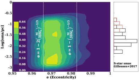
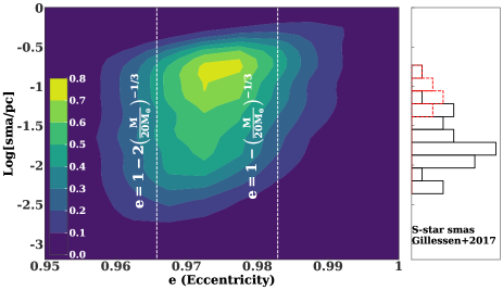
Figure 6: Postdisruption semimajor axis and eccentricity distribution for circular binaries (top) and thermal eccentricity binaries (bottom) from our Monte Carlo ensemble of binary–SMBH encounters. In this case the binary’s center-of-mass orbit is approximated to be parabolic. The dashed, vertical lines show the range of eccentricities predicted analytically (see Equation 26). The histogram on the right shows the observed distribution of S-star semimajor axes from Gillessen et al. (2017); the eight S-stars that are members of the clockwise disk are shown in red.

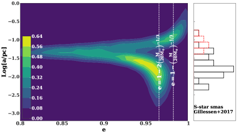
Figure 7: Same as the bottom panel of Fig. 6, except the binary’s center-of-mass is no longer approximated as parabolic. Instead, each binary’s center-of-mass orbit has an eccentricity $e=1-\frac{r_{t}}{a_{d}}$, where $r_{t}$ is the effective tidal radius (Equation 22) and $a_{d}=0.05$ pc is the inner edge of the clockwise disk. Note that in this case both stars can remain bound to the SMBH after a binary disruption.

5.2 Reproducing the number of S-stars

We now check whether the eccentric disk instability could reproduce the observed number of S-stars. Following the logic of the Drake equation (Drake, 1965), we expect

$$N_{s}=N_{d}f_{d}(1-f_{c})$$ (27)

S-stars inside the inner edge of the clockwise disk. Here $N_{d}$ is the number of binaries in the disk, and $f_{d}$ is the fraction of disk stars that have their pericenter pushed below the binary tidal radius. Based on our eccentric disk simulations $f_{d}\lesssim 0.2$. $f_{c}$ is the fraction of binaries that would collide instead of disrupting. Based on our Monte Carlo simulations of binary–SMBH encounters, $f_{c}\approx 0.2$.

We must also account for completeness effects. Dim, low-mass S-stars around $\sim 1M_{\odot}$ are not currently observable. Based on the observed spectra and K-band luminosities (Habibi et al., 2017; Cai et al., 2018), the S-stars have masses between $\sim$3 and 15 $M_{\odot}$. We expect $f_{\rm mf}N_{s}$ S-stars within this mass range. For the $m^{-1.7}$ disk mask function (Lu et al., 2013), $f_{\rm mf}\approx 0.33$.

The total mass of the clockwise disk is inferred to be between $\sim 1.4\times 10^{4}M_{\odot}$ and $3.7\times 10^{4}M_{\odot}$ (Lu et al., 2013). This would imply between 2300 and 6200 stars in the disk (or between $1100$ and $3100$ binaries for a binary fraction of unity). For $N_{d}=1000$, the number of S-stars between 3 and 15 $M_{\odot}$ would be $\mathrel{\hbox to0.0pt{\lower 4.0pt\hbox{\hskip 1.0pt$\sim$}\hss}\raise 1.0pt\hbox{$<$}}50$. Thus, the eccentric disk instability can reproduce the observed number of S-stars.

6 Reproducing the observed eccentricity distribution of the S-stars

We have argued that if the S-stars are sourced by the Hills mechanism, a relaxation process is needed to reproduce their present-day eccentricity distribution. The timescale over which this relaxation occurs is tightly constrained by (i) the observed ages of the S-stars ($\sim 10$ Myr; Habibi et al. 2017), (ii) the age of the clockwise disk ($2.5-5.8$ Myr; Lu et al. 2013), and (iii) the flight time of the Koposov et al. (2020) hypervelocity star from the Galactic center (4.8 Myr).

In this section, we consider three possible relaxation mechanisms: (a) scalar resonant relaxation (b) secular torques from the clockwise disk and (c) an IMBH. We find that the first and third mechanisms can reproduce the observed eccentricity distribution of the S-stars within $10^{7}$ years, as required by observations.

6.1 Resonant relaxation

Resonant relaxation occurs in potentials with a high degree of symmetry, like a Keplerian potential. In a nearly Keplerian potential, orbits will be fixed over many periods. This leads to a coherent buildup of torques on each orbit (Rauch & Tremaine, 1996). These torques can change either the direction or the magnitude of an orbit’s angular momentum. The former is vector resonant relaxation (VRR), and the latter is scalar resonant relaxation (SRR). We focus on SRR, as VRR cannot change an orbit’s eccentricity. However, VRR likely plays an important role in the dynamics of the S-star cluster, as it can change the orientations of the S-stars’ orbits within a few million years (Kocsis & Tremaine, 2011).

The SRR time depends on the precession rate of the stellar orbits. After orbits start to precess, the torques no longer add coherently and the angular momentum evolution becomes a random walk. Orbital precession can be caused by general relativity or by the distributed mass in the star cluster. When orbital precession is dominated by the distributed mass, the SRR time is

$$t_{\rm rr}\propto\frac{M}{\widetilde{m}}P$$

$$\widetilde{m}\equiv\frac{\overline{m^{2}}}{\overline{m}}$$ (28)

where $M$ is the mass of the SMBH, $P$ is the orbital period, and $m$ is the stellar mass. Horizontal bars denote averages (Rauch & Tremaine, 1996; Alexander, 2017). Adding massive perturbers, like black holes, increases $\widetilde{m}$, and decreases the resonant relaxation time. Physically, a clumpier mass distribution increases the rms torque on stellar orbits.

There have been a number of estimates of the SRR time in the Galactic center. Notably, Antonini & Merritt (2013) derived the resonant relaxation time from Monte Carlo simulations, concluding a population of stellar mass black holes can reduce the resonant relaxation time near the present-day location of the S-stars to $\sim 10^{7}$ years, roughly consistent with their observed ages and the time since the hypervelocity star from Koposov et al. (2020) was ejected from the Galactic center.

Here we revisit these estimates in light of new developments in the theory of resonant relaxation. In particular, Bar-Or & Fouvry (2018) derived diffusion coefficients for SRR in a spherical, isotropic cluster from first principles. In their work, the stochastic perturbations of the stellar background on a star are encapsulated as a sum of spherical harmonic noise terms in its orbit-averaged Hamiltonian. The angular momentum diffusion coefficients are related to the autocorrelation function of these terms. Bar-Or & Fouvry (2018) found that SRR is strongly quenched for rapidly precessing eccentric orbits by the adiabatic invariance of the angular momentum, i.e. by the divergence of the relativistic precession frequency as orbits get more and more eccentric.

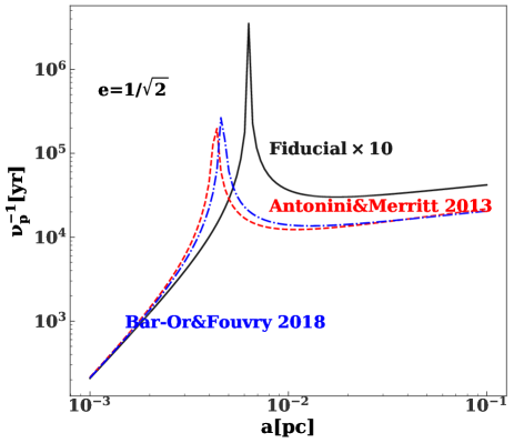
Figure 8: Orbital precession timescale as a function of semimajor axis for different models of the Galactic center. The orbital eccentricity is $1/\sqrt{2}$. The peak in the precession timescale is due to cancellation between prograde GR precession (which dominates on small scales) and retrograde precession due to the distributed mass in the Galactic center (which dominates on large scales).

Figure 9: Left panels: resonant relaxation diffusion coefficient at $a=0.01$ pc (solid black line) and 0.005 pc (dash-dotted gray line) for different models of the Galactic center. The dashed red lines are the second-order nonresonant angular momentum diffusion coefficient. For small angular momentum (inside the Schwarzschild barrier), the angular momentum diffusion coefficient decreases sharply due to general relativistic precession. The vertical, blue lines show the mean angular momentum of bound stars with semimajor axes less than or equal to 0.01 pc in the binary disruption simulations in Figure 7. Right panels: evolution of an example angular momentum distribution function due to resonant and nonresonant relaxation for different Galactic center density profiles. In each case we evolve the angular momentum distribution using Equation (29) with the appropriate diffusion coefficients from the left panels. The dash–dotted lines in the top, right panel show the effects of excluding nonresonant relaxation. The initial distribution function is a Gaussian centered on $j/j_{c}$=0.26 (corresponding to an eccentricity of 0.97, the mean eccentricity expected from binary disruptions). The angular momentum distribution evolves toward a thermal distribution (red dashed line). Note the different snapshot times in the bottom right panel.

The isotropically averaged resonant relaxation time is

$$t_{\rm rr}=\frac{1}{\int_{j_{\rm lc}}^{1}2jD_{jj,RR}(j)dj},$$ (29)

where $j$ is the angular momentum, $D_{jj,RR}$ is the (second-order) SRR diffusion coefficient, and the subscript “lc” denotes the loss cone (Bar-Or & Fouvry, 2018). The angular momentum is normalized to that of a circular orbit with the same energy. The angular momentum diffusion coefficient $D_{jj,RR}(j)$ can be calculated with the publicly available software package SCRRPY.

In practice, the timescale for relaxation will depend on the initial angular momentum distribution, as the resonant relaxation diffusion coefficient is a strong function of the angular momentum. Also, complete thermalization of the S-star orbits may not be required. There are only a few dozen S-stars, so distinguishing a thermal distribution from one that is somewhat superthermal is challenging.

We determine the timescale for scalar resonant relaxation to approximately reproduce the observed S-star eccentricities by solving the angular momentum diffusion equation, viz.

$$\frac{\partial P(j,t)}{\partial t}=\frac{1}{2}\frac{\partial}{\partial j}\left[j(D_{jj,RR}+D_{jj,NRR})\frac{\partial}{\partial j}\left[\frac{P(j,t)}{j}\right]\right],$$ (30)

where $P(j,t)$ is the angular momentum distribution function and $j$ is the specific angular momentum, which we generally normalize by the circular angular momentum $j_{c}$. $D_{jj,NRR}$ is the nonresonant diffusion coefficient (which can be calculated using Appendix C of Bar-Or & Alexander 2016). For the initial conditions, we use the angular momentum distributions from our binary disruption simulations. In particular, the initial distribution function is a Gaussian centered at $j/j_{c}=0.26$ with a standard deviation of $2.4\times 10^{-2}$. We consider a few different diffusion coefficients corresponding to different models for the density of stars and remnants in the Galactic center. First, we consider the Fiducial$\times 10$ model from Generozov et al. (2018). For technical reasons, we use a power-law approximation for the density profile of each component in this model. In this approximation, the mass in stars ($m_{\star}$) and black holes ($m_{\bullet}$) within semimajor axis $a$ is

$$m_{\star}(<a)\approx 7.9\times 10^{3}M_{\odot}\left(\frac{a}{0.1\,\rm pc}\right)^{1.5}$$

$$m_{\bullet}(<a)\approx 3.8\times 10^{4}M_{\odot}\left(\frac{a}{0.1\,\rm pc}\right)^{1.2}.$$ (31)

These profiles are accurate inside of $\sim$0.1 pc where the S-stars are located, but overestimate the number of black holes at larger scales. However, this would not affect the results, as the torque on a particular star is dominated by orbits within a factor of two of its semimajor axis (Gürkan & Hopman, 2007).

We also consider the stellar density profiles from Antonini & Merritt (2013) to more directly compare to this work. They have $1M_{\odot}$ stars and $10M_{\odot}$ black holes with the following profiles:

$$m_{\star}(<a)\approx 6.7\times 10^{4}M_{\odot}\left(\frac{a}{0.1\,\rm pc}\right)^{1.25}$$

$$m_{\bullet}(<a)\approx 2.4\times 10^{4}M_{\odot}\left(\frac{a}{0.1\,\rm pc}\right).$$ (32)

Finally, we consider a simple one-component model with only $1M_{\odot}$ stars from Bar-Or & Fouvry (2018)

$$m_{\star}(<a)\approx 9.4\times 10^{4}M_{\odot}\left(\frac{a}{0.1\,\rm pc}\right)^{1.25}.$$ (33)

The left panels of Fig. 9 show the second-order diffusion coefficient in these models for a couple of different semimajor axes. In all cases, the angular momentum diffusion coefficient falls off inside of some critical angular momentum $j_{\rm crit}$ (this is the “Schwarzschild barrier” from Merritt et al. 2011). Importantly, the location of the Schwarzschild barrier is a function of semimajor axis and the Galactic center density profile, so that binary disruption can deposit stars either inside or outside of it, with a drastic effect on the efficiency of angular momentum diffusion. The variation in $j_{\rm crit}$ is due to differences in the orbital precession rates. As shown by Bar-Or & Fouvry (2018), $j_{\rm crit}$ is where the precession rate of orbits due to GR is equal to the coherence time for the system (that is a representative timescale over which orbits are fixed). Orbits that precess faster than the coherence time will experience no secular torque. The Schwarzschild barrier, $j_{\rm crit}$, can be estimated from the following equation

$$\nu_{\rm gr}(a,j_{\rm crit})=\frac{0.45}{T_{c}(a)}$$

$$T_{c}\equiv\sqrt{\frac{\pi}{2}}\nu_{p}^{-1}(2a),$$ (34)

where $a$ is the semimajor axis, $\nu_{\rm gr}(a,j_{\rm crit})$ is the orbital precession frequency due to GR, and $T_{c}$ is the coherence time for resonant relaxation. For a spherical, isotropic population the coherence time is the total orbital precession frequency $\nu_{p}$ evaluated at a semimajor axis of $2a$, and an eccentricity of $1/\sqrt{2}$. This precession rate depends on the distributed mass profile within the Galactic center. Figure 8 shows the precession rate as a function of semimajor axis for the models considered here.

Inside of the Schwarzschild barrier, nonresonant relaxation can be more efficient than resonant relaxation, as shown by the dashed red lines in the left panels of Fig. 9.

The right panels of Fig. 9 show the evolution of the “Hills injected distribution” at a semimajor axis of 0.01 pc for different Galactic center models (equations 31, 32, and 33). The Fiducial$\times$10 and Antonini & Merritt (2013) models have similar isotropically average resonant relaxation times at 0.01 pc (see Fig. 10). However, the evolution is faster for the Antonini & Merritt (2013) model, as binary disruptions deposit stars closer to the Schwarzschild barrier.

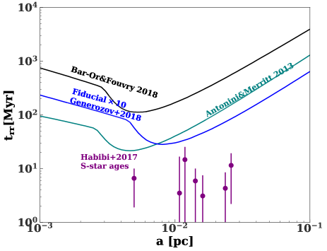
Figure 10: Isotropically averaged scalar resonant relaxation time (Equation 29) as a function of semimajor axis. Different colors correspond to different models for the stellar density profile in the Galactic center (see the text for details). The purple points are the measured ages of eight of the S-stars from Habibi et al. (2017).

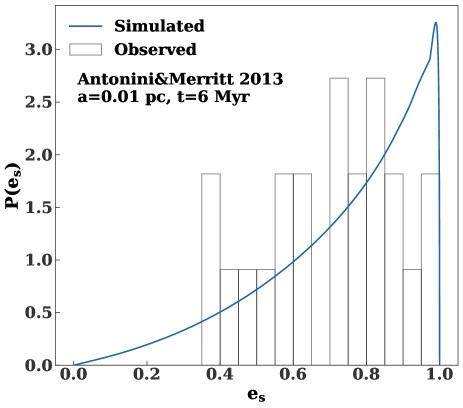
Figure 11: Eccentricity distribution at 0.01 pc in the Antonini & Merritt (2013) model after 6 Myr of evolution (blue line). This is the earliest snapshot for this model that is consistent with the observed eccentricity distribution of the S-stars (black, empty, histogram).

Table 2: Approximate Timescale Required to Reproduce the Observed S-star Eccentricities for Different Models of the Galactic Center Compared to the Isotropically Averaged Resonant Relaxation Time (Equation 29).

	a=0.005 pc			a=0.01 pc
	Timescale to reproduce S-stars	$t_{\rm rr}$		Timescale to reproduce S-stars	$t_{\rm rr}$
Model	(Myr)	(Myr)		(Myr)	(Myr)
Fiducial$\times$10	13	57		8	30
Antonini&Merritt 2013	7	22		6	40
Bar-Or&Fouvry 2018	41	110		24	170

We compare the evolving distribution functions in Fig. 9 to the eccentricities of the 22 S-stars with semimajor axes less than or equal to 0.03 pc from Table 3 of Gillessen et al. (2017). Specifically, we identify the earliest time where (i) the Kolmogorov–Smirnov (KS) test probability that the observed S-star eccentricities are consistent with the simulated distribution is at least 10% and (ii) there is at least a five percent probability that there are two or fewer stars with eccentricities greater than equal to 0.95 as in the observed S-stars. Although simulated distributions correspond to one fixed semimajor axis, we always compare to the entire S-star sample within 0.03 pc. Table 2 shows the timescales required to satisfy these criteria for different Galactic center density profiles. Fig. 11 shows a comparison between the observed S-star eccentricity distribution and a snapshot from the solutions in Fig. 9. This snapshot is the earliest one in the Antonini & Merritt (2013) model where the above statistical criteria are satisfied. Overall, resonant relaxation can reproduce the observed S-star eccentricity distribution within $\sim 10$ Myr assuming a realistic population of stellar mass black holes.

6.2 Disk torques

In this section, we quantify secular torques from the clockwise disk to see if they could thermalize the S-star eccentricity distribution. First, we quantify the expected torque analytically. The torque on a particle well inside of the disk may be estimated via spherical harmonic expansion, as shown below.

First, we replace the disk with a single particle of mass $M_{d}$ on an elliptical orbit around the central SMBH. The spherical harmonic expansion of this orbit’s gravitational potential at a point $\mathbf{r}$ with spherical polar coordinates $<r,\theta,\phi>$ is

$$U_{\rm\ell m}=-GM_{d}\sum_{\ell=0}^{\infty}\sum_{m=-\ell}^{\ell}W_{\ell m}r^{\ell}Y_{\ell}^{m}(\theta,\phi)\frac{\exp[-im\Phi]}{D^{\ell+1}},$$ (35)

where $\Phi$ is the true anomaly of the particle, $D$ is its distance from the center, and $Y_{\ell}^{m}$ is the spherical harmonic of degree $\ell$, $m$ (see, e.g., equation 3 of Fuller & Lai 2011). Here $W_{\ell m}$ is a constant and is nonzero only if $\ell+m$ is even. The physical potential is the real part of the above expression.

The orbit-averaged $\ell,m$ component of the potential is

$$\left<U_{\ell m}\right>=\frac{\int_{0}^{2\pi}U_{\ell m}(D,\Phi)\frac{d\Phi}{\dot{\Phi}}}{P_{\rm orb}},$$ (36)

where $P_{\rm orb}$ is the orbital period and

$$D=\frac{a_{d}(1-e_{d}^{2})}{1+e_{d}\cos(\Phi)}$$ (37)

$$\dot{\Phi}=\frac{j_{d}}{D^{2}},$$ (38)

where $a_{d}$, $e_{d}$, $j_{d}$ are the semimajor axis, eccentricity, and the specific angular momentum of the disk orbit respectively ($j_{d}={\rm Constant}\times\sqrt{a_{d}(1-e_{d}^{2})}$ ).

The $\ell=0$ term does not depend on $\mathbf{r}$, and therefore does not contribute any force. The orbit–average of the $\ell=1$ and the $\ell=2,m=\pm 2$ terms is 0.

The orbit average of the $\ell=2,m=0$ component is nonzero, but the corresponding force is radial in the plane of the orbit and would exert no torque. The leading-order contribution to the torque comes from the $\ell,m=3,\pm 1$ terms of the potential expansion. In the plane of the orbit (where $\theta=\pi/2$), the $\phi$ component of the specific force from these terms is

$$<f_{3,1}>= \frac{3}{8}GM_{d}\sin(\phi)\frac{e_{d}r^{2}}{a_{d}^{4}(1-e_{d}^{2})^{5/2}}$$ (39)

The corresponding specific torque is

$$<\tau_{3,1}>= \frac{3}{8}\underbrace{\frac{GM_{d}}{a_{d}}}_{\tau_{d}}\sin(\phi)\frac{e_{d}}{(1-e_{d}^{2})^{5/2}}\frac{r^{3}}{a_{d}^{3}}$$ (40)

Thus, the torques fall off as $r^{3}$ within the inner edge of the disk. The torque on a test orbit at an angle $\overline{\omega}$ with respect to the disk is

$$<<\tau_{3,1}>>=f(e^{\prime})\tau_{d}\frac{e_{d}}{(1-e_{d}^{2})^{5/2}}\left(\frac{a^{\prime}}{a_{d}}\right)^{3}\sin(\overline{\omega}),$$ (41)

where the $a^{\prime}$ and $e^{\prime}$ are the semimajor axis and eccentricity of the test orbit. The double brackets on the left side of the above equation denote averages over the disk and test orbits. If the test star was injected via the Hills mechanism, $e^{\prime}\sim 0.97$ and $f(e^{\prime})=1.6$.

For the S-stars $a^{\prime}/a_{d}\approx 0.2$, and $<<\tau_{3,1}>>\approx 4.7\times 10^{-2}\tau_{d}$ for $e_{d}=0.7$. Here $\tau_{d}$ is the characteristic torque at the inner edge of the disk. If the S-star and disk orbits remained static, even this attenuated torque could perturb the S-stars’ eccentricities significantly over their lifetime. For a star with a semimajor axis of 0.01 pc and an eccentricity of 0.97, the characteristic time–scale to perturb its angular momentum is $j/<<\tau_{3,1}>>\approx 8\times 10^{4}$ years.

However, the torques from the disk would be further attenuated by precession of the disk and S-star orbits. The top panel of Fig. 12 shows the specific torque on an $e^{\prime}=0.97$, $a^{\prime}=0.01$ pc test orbit inside of an idealized, non–precessing eccentric disk with $e_{d}=0.7$, $a_{d}=0.05$ pc, and a total mass of $10^{4}M_{\odot}$. Here GR causes the highly eccentric test orbit to precess $2\pi$ radians over $4.7\times 10^{4}$ years. In principle, the test orbit’s eccentricity (and precession rate) are allowed to change. In practice, the torque frequently reverses in sign, so the test orbit’s eccentricity is nearly constant, as shown in the bottom panel of Fig. 12.

The eccentric disk will also evolve over time. We include this effect by directly injecting remnant stars after binary disruptions in N-body simulations of an eccentric disk (see $\S$ 2 for a description of the basic simulation setup). Specifically, whenever a particle crosses the tidal radius in a simulation it is replaced with a child particle with a semimajor axis of $a^{\prime}=0.01$ pc, and an eccentricity of $e^{\prime}=1-r_{p}/a^{\prime}$. All of the other orbital elements are inherited from the parent. For computational convenience, the child particles are taken to be massless.

The curves in Fig. 13 show the postdisruption evolution of the injected particles’ eccentricities compiled from several simulations. The injected stars retain eccentricities greater than 0.96 over 5 Myr.

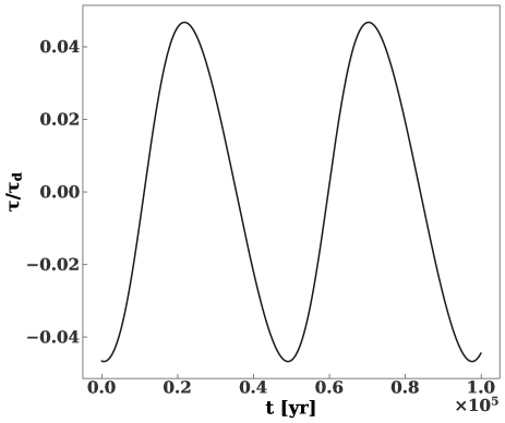
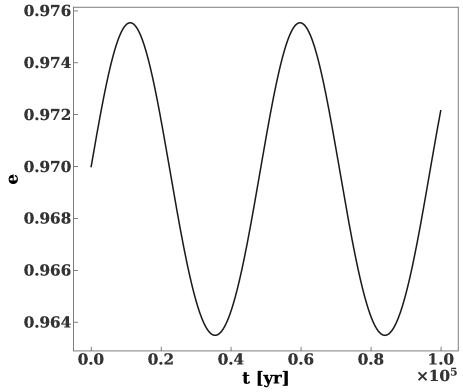
Figure 12: Top panel: torque from an idealized eccentric disk on a test orbit with a semimajor axis of 0.01 pc and an initial eccentricity 0.97 as a function of time (see text for details). The torque is normalized by $\tau_{d}=\frac{Gm_{\rm d}}{a_{\rm d}}$, where $a_{\rm d}$ and $m_{\rm d}$ are the characteristic semimajor axis and the mass of the disk, respectively. The semimajor axis of this test orbit is five times smaller than the inner edge of the disk. The test orbit experiences general relativistic precession, so that the torque rapidly changes sign, and the eccentricity oscillates as shown in the bottom panel.

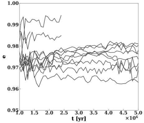
Figure 13: Eccentricity evolution of a set of test particles injected into N-body simulations of an eccentric disk (see Fig. 1). These particles are injected after binary disruptions in the simulations and start with an eccentricity of $\sim 0.97$ and a semimajor axis of 0.01 pc, which is five times smaller than the inner edge of the disk. Note that these data are compiled from multiple simulations.

6.3 Effect of IMBHs

In this section, we demonstrate that an $\sim 10^{3}M_{\odot}$ IMBH with a semimajor axis of $\sim$0.01 pc could thermalize the eccentricity distribution of stars deposited via the Hills mechanism. Such IMBHs may originate from globular clusters. In particular, IMBHs may form from runaway black hole mergers in very dense globular clusters (Antonini et al., 2019) or other types of collisional runaways (Ebisuzaki et al., 2001; Portegies Zwart & McMillan, 2002; Gürkan et al., 2004; Freitag et al., 2006; Goswami et al., 2012). Fragione et al. (2018a, b) studied the evolution of globular clusters with a primordial IMBH. In the Milky Way, most such IMBHs would be orphaned from their parent cluster (either by gravitational wave recoil kicks or tidal dissolution of the surrounding cluster), leaving a population of $\sim 1000$ bare IMBHs within the central kpc of the Galaxy. These IMBHs may then inspiral toward the Galactic center via dynamical friction. Past work has shown that IMBHs would stall at $\sim 0.01(q/10^{-3})$ pc from the Galactic center (where $q$ is the mass ratio between the IMBH and the central SMBH; see Merritt et al. 2009 and the references therein). As the IMBH is closer to the S-stars than the clockwise disk, it is more effective at changing their eccentricity distribution.

We now review existing observational and theoretical constraints on the presence of an IMBH in the Galactic center. Proper-motion studies of Sgr A* can rule out an IMBH with mass $\mathrel{\hbox to0.0pt{\lower 4.0pt\hbox{\hskip 1.0pt$\sim$}\hss}\raise 1.0pt\hbox{$>$}}10^{4}M_{\odot}$ 0.01 pc from the Galactic center (Reid & Brunthaler, 2020). Additionally, an IMBH of $10^{3}M_{\odot}$ inside of $1.3\times 10^{-4}$ pc would inspiral into the central SMBH in less than 10 Myr due to gravitational wave emission (e.g. Gualandris & Merritt 2009).

Recently, Naoz et al. (2020) used observations of S2 to place stringent constraints on the presence of an IMBH in the Galactic Center. They found that a $10^{5}M_{\odot}$ IMBH cannot have a semimajor axis greater than 170 au ($8.2\times 10^{-4}$ pc). For a $10^{3}M_{\odot}$ they found the maximum semimajor axis from observational constraints is $\sim 1000$ au ($5\times 10^{-3}$ pc).

However, an IMBH at 0.01 pc is no longer inside of the orbit of S2, as assumed in Naoz et al. (2020). Also, in this case the IMBH-SMBH-S2 system is not longer strongly hierarchical. Therefore, we perform direct three-body integrations with REBOUND (with the “GR” effect included) to see what effect an $10^{3}M_{\odot}$ IMBH at 0.01 pc would have on the orientation of S2’s orbit. We find that that orbital precession rate is $\approx 0.01$ degrees per year in the case, which is consistent with existing observational limits (note this is also the precession rate expected from GR effects alone). We also find a $10^{5}M_{\odot}$ IMBH at 170 au would cause S2 to precess by a few tenths of a degree per year and can be ruled out from observations (as expected from Naoz et al. 2020).

As we were completing revisions to this paper, the GRAVITY collaboration reported a detection of apsidal precession in S2’s orbit. The detected precession is consistent with that expected from GR alone (Gravity Collaboration et al., 2020). Combining the the latest constraints on S2’s orbit with N-body simulations of an IMBH interacting with the S-star cluster (Gualandris et al., 2010), they find IMBH masses $\mathrel{\hbox to0.0pt{\lower 4.0pt\hbox{\hskip 1.0pt$\sim$}\hss}\raise 1.0pt\hbox{$>$}}10^{3}M_{\odot}$ are ruled out at 0.01 pc.

We perform N-body simulations with AR--Chain of 20 ten solar mass stars interacting with an IMBH. Merritt et al. (2009) and Gualandris & Merritt (2009) performed similar calculations. However, in our simulations, the stars are initially on highly eccentric orbits with $e\approx 0.97$, as expected from the Hills mechanism. More precisely, we draw the stars’ semimajor axis ($a$) and eccentricity from a distribution similar to that in Fig. 6, with the restriction $0.005\,{\rm pc}\leq a\leq 0.03\,{\rm pc}$. The stars are all initially in a plane with a randomized orientation and mean anomaly. We consider four different IMBH masses ($M_{\rm IMBH}$) between $3\times 10^{2}M_{\odot}$ and $10^{4}M_{\odot}$, five different inclinations ($i_{\rm imbh}$) evenly spaced between $5.7^{\circ}$ and $174.3^{\circ}$, and two eccentricities (0, 0.7). We perform four different $\sim 10$ Myr simulations for each set of IMBH parameters. Post-Newtonian effects are included for the black holes in these simulations up to a PN order of 2.5. The IMBH parameters in our simulations are summarized in Table 3.

Table 3: IMBH Parameters for the Simulations in This Section.

$M_{\rm IMBH}$	$3\times 10^{2}$, $10^{3}$, $3\times 10^{3}$, $10^{4}M_{\odot}$
$i_{\rm IMBH}$	$5.7$, $48$, $90$, $132$, $174^{\circ}$
$e_{\rm IMBH}$	0, 0.7

Note. — The semimajor axis is fixed to 0.01 pc for simplicity.

To identify IMBH parameters that would reproduce the observations, we find snapshots where the following criteria are met.

1. At least half of the simulated S-stars remain within 0.03 pc.

2. The KS and Anderson–Darling test probabilities that the simulated and observed S-star eccentricity distributions are consistent is at least 10%.

3. There are no more than two stars with eccentricity greater than 0.95, as in the observed population. For this and the preceding condition, we only consider stars with semimajor axes within 0.03 pc

4. The preceding criteria are met at least 5% of the time after 4 Myr.

The last condition is motivated by the best-fit age of the clockwise disk from Lu et al. (2013), and the (4.8 Myr) flight time of the Koposov et al. (2020) hypervelocity star. (In the eccentric disk scenario, most binary disruptions occur within $\sim 1$ Myr of disk formation; see Fig. 3). The most massive IMBHs in our grid ($3\times 10^{3}M_{\odot}$ and $10^{4}M_{\odot}$) violate the first condition after 4 Myr, but $3\times 10^{3}M_{\odot}$ IMBHs can be effective on shorter time–scales.

Table 4 summarizes the IMBH parameters for which at least one of the four simulations we ran satisfies the above conditions. For circular IMBHs, only simulations with $M_{\rm IMBH}=10^{3}M_{\odot}$ and $i_{\rm imbh}=5.7^{\circ}$ or $i_{\rm imbh}=48^{\circ}$ satisfy all of the above criteria. A $10^{3}M_{\odot}$ IMBH with an eccentricity of 0.7 satisfies the criteria for all inclinations in our grid except for 48^∘. Finally, one simulation with an eccentric $300M_{\odot}$ IMBH at an inclination of $5.7^{\circ}$ satisfies these conditions. As shown in the last two columns, these IMBHs can generally thermalize the S-stars’ eccentricity distribution over a few Myr, as required by observations.

Table 4: IMBH Parameters that Can Reproduce the Observed S-star Eccentricity Distribution, According to the Criteria Above.

$M_{\rm IMBH}$	$i_{\rm IMBH}$	$e_{\rm IMBH}$	$t_{\rm min}$	$t_{\rm max}$	Mergers
$(M_{\odot})$	(deg)		(Myr)	(Myr)
$3\times 10^{2}$	5.7	0.7	6.1	10	0
$10^{3}$	5.7	0	3.5	8.5	2
$10^{3}$	48	0	7.3	9.4	1
$10^{3}$	5.7	0.7	4.3	9.9	0
$10^{3}$	90	0.7	2.4	9.8	2
$10^{3}$	132	0.7	2.3	10	0
$10^{3}$	174	0.7	1.8	9.9	1–4

Note. — The fourth and fifth columns are the minimum and maximum times for which the first three criteria are satisfied. The last column shows the number of mergers (with respect to the SMBH) recorded in the simulation.

The blue filled histograms in Fig. 14, show the eccentricity, semimajor axis, and inclination distributions from an example simulation snapshot where the above conditions are satisfied. The black open histograms in this figure show the distribution of the S-stars with semimajor axes inside of 0.03 pc. As shown in Fig. 15, the eccentricity distribution from this simulation is statistically consistent with observations for a range of times. Note that the distributions in Fig. 14 only include stars with semimajor axes inside of 0.03 pc. Some stars in our simulations are kicked to larger semimajor axes. However, interactions with the clockwise disk (which are not included in these simulations), would be important for these stars.

In this case the IMBH also isotropizes the S-star orbits, so that their inclination distribution is consistent with observations. In general, the IMBHs in Table 4 can isotropize the S-star orbits, except for the those with the lowest inclinations ($i=5.7^{\circ}$). However, as discussed in § 6, vector resonant relaxation can also isotropize the S-star orbits.

Finally, zero to two stars are unbound from the SMBH in these simulations. Also, a few “mergers” were recorded between stars and the central SMBH as summarized in the last column of Table 4.

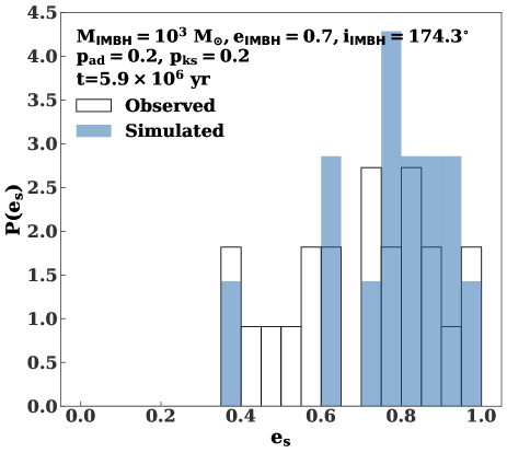
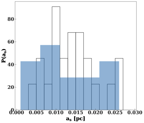
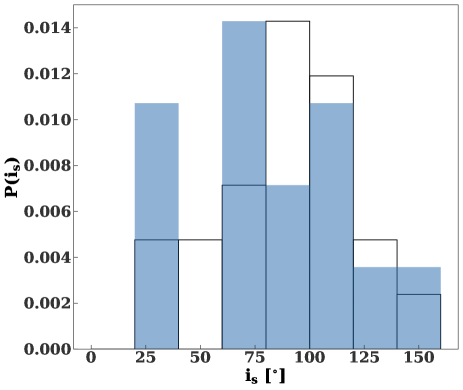
Figure 14: Snapshot of orbital element distributions from an N-body simulation of 10 $M_{\odot}$ stars interacting with an IMBH with the parameters in the top panel (blue filled histogram). The stars all have an initial eccentricity $\mathrel{\hbox to0.0pt{\lower 4.0pt\hbox{\hskip 1.0pt$\sim$}\hss}\raise 1.0pt\hbox{$>$}}$0.96. The observed eccentricity distribution of the S-stars from Gillessen et al. (2017) is shown by the black open histogram. The panels show eccentricity (top left), semimajor axis (top right), and inclination (bottom). $p_{\rm KS}$ and $p_{\rm AD}$ are the two-sample KS and and Anderson–Darling test p-values that the simulated and observed eccentricity distributions are consistent. Note that for this plot, we exclude stars with semimajor axes greater than 0.03 pc.

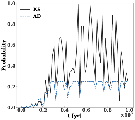
Figure 15: KS (black solid) and Anderson–Darling (AD) (blue dashed) probabilities that the eccentricities from the simulation in Fig. 14 are consistent with the observed S-star eccentricities as a function of time. Note that implementation we use for the latter (“anderson_ksamp” in scipy.stats) caps the probability at 0.25.

7 Discussion

7.1 Stellar collisions

Approximately 20% percent of our simulated binary–SMBH encounters result in collisions between stars rather than tidal separation of the binary. Table 5 shows the fraction of encounters that result in collisions for different binary eccentricity distributions. We consider stars to have collided if they enter into Roche lobe contact during the encounter with the SMBH (see Equation 10).

The above statistics are based on one simulated encounter with the central SMBH per binary. However, if binaries are in the empty loss cone, they would approach the tidal radius gradually over several orbits (see § 2.1). In this process, the binary could be excited to high eccentricities so that the stars collide before the binary is disrupted (Antonini et al., 2010; Bradnick et al., 2017). This would increase the ratio of collisions to disruptions. However, Antonini et al. (2010) find that most additional collisions would come from highly inclined binaries due to Kozai–Lidov resonances. Therefore, this effect would not be present in our assumed coplanar configuration.

The ultimate fate of binaries that do collide depends on the collision velocity. If this is smaller than the stellar escape speed, a merger will result. For faster collisions, tidal separation of the binary can still occur (Ginsburg & Loeb, 2007). Binaries that do merge may account for G2-like objects (Witzel et al., 2014).

Table 5: Fraction of Monte Carlo Binary–SMBH Simulations Resulting in Binary Disruptions (Column 1), Collisions (Column 2), and the Ratio of Collisions to Disruptions (Column 3).

Eccentricity	Percent of Trials Resulting in Disruptions	Percent of Trials Resulting in Collisions	Collisions/Disruptions
Circular	50	20	0.40
Thermal	49	16	0.33

7.2 Hypervelocity stars

Many binary disruptions would result in a hypervelocity star ejected from the Galactic center. The distribution of semimajor axes in Fig. 6 can be directly translated into a distribution of ejection velocities for such stars. For a given S-star semimajor axis $a_{s}$, the ejection velocity of the corresponding hypervelocity star is

$$v_{ej}=\sqrt{\frac{GMm_{\rm s}}{a_{s}m_{\rm ej}}},$$ (42)

where $M$ is the SMBH mass, and we have assumed the initial center-of-mass orbit of the binary was parabolic. Fig. 16 shows the velocity distribution of ejected stars from binaries with a thermal eccentricity distribution (that is the model that best reproduces the observed S-star semimajor axis distribution). For comparison, we also show the velocity of the hypervelocity star detected by Koposov et al. (2020). This star is in the 92nd percentile of the velocity distribution. If we instead use the distribution in Fig. 7, where the binaries’ center of mass has a more realistic eccentricity, this star moves to the 86th percentile of the velocity distribution. In this case the ejected velocity is

$$v_{\rm ej}=\sqrt{\frac{-GMm_{\rm bin}}{m_{\rm ej}a_{d}}+\frac{GMm_{\rm s}}{a_{s}m_{\rm ej}}},$$ (43)

$a_{d}\approx 0.05$ pc is the initial semimajor axis of the binary’s center-of-mass orbit.

Finally, for the ensemble of circular binary disruptions (see the top panel of Fig. 6), the Koposov star would be in the 67th percentile of the velocity distribution.

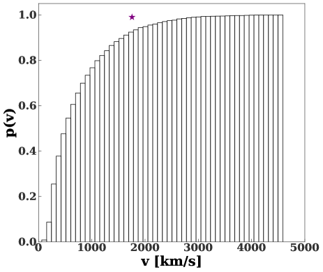
Figure 16: Cumulative velocity distribution for ejected stars in our Monte Carlo ensemble of binary–SMBH encounters (for binaries drawn from a thermal eccentricity distribution). The purple star shows the ejection velocity for the recently discovered hypervelocity star originating from the Galactic Center (Koposov et al., 2020).

7.3 Masses of the S-stars

We have proposed here that the S-stars originally come from the clockwise disk. However, the clockwise disk has O-stars, while the S-stars are all B stars with masses $\mathrel{\hbox to0.0pt{\lower 4.0pt\hbox{\hskip 1.0pt$\sim$}\hss}\raise 1.0pt\hbox{$<$}}15M_{\odot}$ (Habibi et al., 2017).

The simplest explanation would be a sampling effect: there are relatively few S-stars, and by chance no O-star binaries were disrupted. The chances that a random disk star has a mass below $\sim 15M_{\odot}$ is

$$p=\frac{\int_{1M_{\odot}}^{15M_{\odot}}m^{-1.7}dm}{\int_{1M_{\odot}}^{60M_{\odot}}m^{-1.7}dm},$$ (44)

where we assume that the stars are drawn from the observed mass function in Lu et al. (2013), and that this mass function extends from 1 $M_{\odot}$ to the main-sequence turnoff at the age of the disk ($\sim 4$ Myr). There are 22 S-stars inside of 0.03 pc. The chances that they would all be below 15 $M_{\odot}$ is $p^{22}\approx 10\%$, which suggests sampling effects could be a plausible explanation for the mass discrepancy between the S-stars and the clockwise disk. However, the observed S-stars do not include any stars with masses of $\sim 1M_{\odot}$, which are too dim to detect. The dimmest S-star in Table 3 of Gillessen et al. (2017) has a K-band magnitude of 17.8, which suggests a stellar mass of $\sim 3M_{\odot}$ according to Table 1 of Cai et al. (2018). Assuming only stars with masses $\mathrel{\hbox to0.0pt{\lower 4.0pt\hbox{\hskip 1.0pt$\sim$}\hss}\raise 1.0pt\hbox{$>$}}3M_{\odot}$ could be observed, a total of $\sim$50 disruptions are required to produce the observed S-stars, and the probability that none of these disruptions include O stars is $\sim 0.5\%$.

However, the Hills mechanism has a built-in bias, and deposits massive stars at larger semimajor axes. From Equation (25), after the disruption, the bound star has a semimajor axis of

$$a_{s}=\frac{\chi^{2}}{k^{\prime}}\frac{m_{s}}{m_{\rm bin}}\frac{(1+q)^{2}}{2q}\left(\frac{M}{m_{\rm bin}}\right)^{2/3}a_{\rm bin}=$$

$$\begin{cases}\frac{1}{k}\frac{1+q}{2q}\left(\frac{M}{m_{\rm bin}}\right)^{2/3}a_{\rm bin}&{\rm if\,\,primary}\\ \frac{1}{k}\frac{1+q}{2}\left(\frac{M}{m_{\rm bin}}\right)^{2/3}a_{\rm bin}&{\rm if\,\,secondary}.\\ \end{cases}$$ (45)

The semimajor axis of the bound star is a factor of $1/q$ larger if it is the primary. (Note that in the limit of parabolic disruptions the primary and secondary have an equal probability to be left bound to the SMBH; see Sari et al. 2010; Kobayashi et al. 2012.) This effect could explain the dearth of O-stars among the S-stars. We leave a detailed exploration to future work.

8 Conclusion

Recent observations suggest a common origin for the S-star cluster and the clockwise disk in the Galactic center. In particular, recent spectral observations suggest that these two populations have consistent ages (Habibi et al., 2017). Additionally, Koposov et al. (2020) discovered a hypervelocity star that was ejected from the Galactic center 4.8 Myr ago (approximately when the clockwise disk was forming). This strongly suggests that stellar binaries from the clockwise disk were tidally disrupted by the central SMBH early in its history, which would leave a compact cluster of stars inside of the disk (like the S-stars). Disk binaries can be pushed to tidal disruption via a gravitational instability in the disk (Madigan et al., 2009). We perform a detailed study of this scenario. Our results are summarized as follows.

1. We quantify the plausible range of semimajor axes of binary stars in the clockwise disk (see Fig. 4). We find that the evaporation of such binaries is dominated by other disk stars, rather than the isotropic star cluster in the Galactic center.

2. We simulate a large number of encounters between disk binaries and the central SMBH. Tidal disruption of binary stars can reproduce the present-day semimajor axis distribution of the S-stars.

3. The eccentricity distribution of the S-stars is more difficult to reproduce. If these stars are injected via tidal disruption of binaries, they would start with a large eccentricity ($e\sim 0.97$). In contrast, the S-stars have a roughly thermal eccentricity distribution.

4. We have considered three possible mechanisms to thermalize the S-star eccentricity: (a) scalar resonant relaxation (b) torques from the parent clockwise disk, and (c) an IMBH. The flight time of the hypervelocity star discovered by Koposov et al. (2020) and the observed ages of the S-stars require that the S-stars reach their current distribution in $\mathrel{\hbox to0.0pt{\lower 4.0pt\hbox{\hskip 1.0pt$\sim$}\hss}\raise 1.0pt\hbox{$<$}}10^{7}$ years. This is a challenge, as highly eccentric orbits experience rapid general relativistic precession, which suppresses secular torques. We find that torques from the clockwise disk are unlikely to be effective on this timescale. However, scalar resonant relaxation by the isotropic cluster can reproduce the observed eccentricity distribution of S-stars within $10^{7}$ years. Also, a $\sim 10^{3}M_{\odot}$ IMBH at $\sim 0.01$ pc, could reproduce the S-star eccentricity distribution within a few million years. However, such IMBHs are, at best, marginally consistent with the latest observational limits (Gravity Collaboration et al., 2020).

5. After a binary is tidally disrupted, the primary and secondary have equal chances to remain bound to the SMBH (for parabolic disruptions). However, the primary is deposited at larger semimajor axes, which could explain the dearth of O stars among the S-stars.

Appendix A Hills Approximation

In the Hills approximation the time derivative of the binary separation is (Sari et al., 2010)

$$\dot{\mathbf{r}}=\left(\frac{r_{p}}{r_{m}}\right)^{3}\left[-\mathbf{r}+3(\mathbf{r}\cdot\hat{\mathbf{r}}_{m})\hat{\mathbf{r}}_{m}\right]-\frac{\mathbf{r}}{r^{3}},$$ (A1)

where $\mathbf{r}_{m}$ is the unperturbed center-of-mass orbit and $r_{p}$ is the pericenter distance. All distances and times are in units of $\left(\frac{m_{\rm bin}}{M}\right)^{1/3}r_{p}$ and $\sqrt{r_{p}^{3}/GM}$, respectively. Solving the above equation gives the separation of the binary stars as a function of time. We can then use this separation to solve the positions of the individual stars. We call this second step the “Iterated Hills Approximation.”

The postdisruption orbital elements from the Hills approximation are in good agreement with the results from three-body integrations. For deeply penetrating disruptions ($r_{p}\ll r_{t}$) the separations from these two methods diverge when the binary is near pericenter as shown in Fig. 17. However, the two solutions converge again at late times. The positions of the individual stars from the “Iterated Hills Approximation” give a revised estimate for the binary separation. This revised estimate always always falls within $\lesssim$1% of the AR--Chain solution in Fig. 17.

Figure 17: Binary separation for an example disruption. The top line is the solution from the Hills approximation, while the bottom line shows the solutions from AR--Chain and the iterated Hills approximation (see text for details).

References

- Alexander et al. (2017) Alexander, K. D., Wieringa, M. H., Berger, E., Saxton, R. D., & Komossa, S. 2017, ApJ, 837, 153, doi: 10.3847/1538-4357/aa6192
- Alexander (2017) Alexander, T. 2017, ARA&A, 55, 17, doi: 10.1146/annurev-astro-091916-055306
- Alexander & Pfuhl (2014) Alexander, T., & Pfuhl, O. 2014, ApJ, 780, 148, doi: 10.1088/0004-637X/780/2/148
- Antonini et al. (2010) Antonini, F., Faber, J., Gualandris, A., & Merritt, D. 2010, ApJ, 713, 90, doi: 10.1088/0004-637X/713/1/90
- Antonini et al. (2019) Antonini, F., Gieles, M., & Gualandris, A. 2019, MNRAS, 486, 5008, doi: 10.1093/mnras/stz1149
- Antonini & Merritt (2013) Antonini, F., & Merritt, D. 2013, ApJ, 763, L10, doi: 10.1088/2041-8205/763/1/L10
- Antonini & Perets (2012) Antonini, F., & Perets, H. B. 2012, ApJ, 757, 27, doi: 10.1088/0004-637X/757/1/27
- Bar-Or & Alexander (2016) Bar-Or, B., & Alexander, T. 2016, ApJ, 820, 129, doi: 10.3847/0004-637X/820/2/129
- Bar-Or & Fouvry (2018) Bar-Or, B., & Fouvry, J.-B. 2018, ApJ, 860, L23, doi: 10.3847/2041-8213/aac88e
- Bartko et al. (2009) Bartko, H., Martins, F., Fritz, T. K., et al. 2009, ApJ, 697, 1741, doi: 10.1088/0004-637X/697/2/1741
- Bonnell & Rice (2008) Bonnell, I. A., & Rice, W. K. M. 2008, Science, 321, 1060, doi: 10.1126/science.1160653
- Bradnick et al. (2017) Bradnick, B., Mandel, I., & Levin, Y. 2017, MNRAS, 469, 2042, doi: 10.1093/mnras/stx1007
- Cai et al. (2018) Cai, R.-G., Liu, T.-B., & Wang, S.-J. 2018, arXiv e-prints, arXiv:1808.03164. https://arxiv.org/abs/1808.03164
- Do et al. (2013) Do, T., Lu, J. R., Ghez, A. M., et al. 2013, ApJ, 764, 154, doi: 10.1088/0004-637X/764/2/154
- Drake (1965) Drake, F. D. 1965, The Radio Search for Intelligent Extraterrestrial Life, 323–345
- Dremova et al. (2019) Dremova, G. N., Dremov, V. V., & Tutukov, A. V. 2019, Astronomy Reports, 63, 862, doi: 10.1134/S1063772919100032
- Ebisuzaki et al. (2001) Ebisuzaki, T., Makino, J., Tsuru, T. G., et al. 2001, ApJ, 562, L19, doi: 10.1086/338118
- Eggleton (1983) Eggleton, P. P. 1983, ApJ, 268, 368, doi: 10.1086/160960
- Foote et al. (2020) Foote, H. R., Generozov, A., & Madigan, A.-M. 2020, ApJ, 890, 175, doi: 10.3847/1538-4357/ab6c66
- Fragione & Antonini (2019) Fragione, G., & Antonini, F. 2019, MNRAS, 488, 728, doi: 10.1093/mnras/stz1723
- Fragione et al. (2017) Fragione, G., Capuzzo-Dolcetta, R., & Kroupa, P. 2017, MNRAS, 467, 451, doi: 10.1093/mnras/stx106
- Fragione et al. (2018a) Fragione, G., Ginsburg, I., & Kocsis, B. 2018a, ApJ, 856, 92, doi: 10.3847/1538-4357/aab368
- Fragione et al. (2018b) Fragione, G., Leigh, N. W. C., Ginsburg, I., & Kocsis, B. 2018b, ApJ, 867, 119, doi: 10.3847/1538-4357/aae486
- Fragione & Sari (2018) Fragione, G., & Sari, R. 2018, ApJ, 852, 51, doi: 10.3847/1538-4357/aaa0d7
- Freitag et al. (2006) Freitag, M., Gürkan, M. A., & Rasio, F. A. 2006, MNRAS, 368, 141, doi: 10.1111/j.1365-2966.2006.10096.x
- Fuller & Lai (2011) Fuller, J., & Lai, D. 2011, MNRAS, 412, 1331, doi: 10.1111/j.1365-2966.2010.18017.x
- Generozov et al. (2018) Generozov, A., Stone, N. C., Metzger, B. D., & Ostriker, J. P. 2018, MNRAS, 478, 4030, doi: 10.1093/mnras/sty1262
- Ghez et al. (2003) Ghez, A. M., Duchêne, G., Matthews, K., et al. 2003, ApJ, 586, L127, doi: 10.1086/374804
- Gillessen et al. (2017) Gillessen, S., Plewa, P. M., Eisenhauer, F., et al. 2017, ApJ, 837, 30, doi: 10.3847/1538-4357/aa5c41
- Ginsburg & Loeb (2006) Ginsburg, I., & Loeb, A. 2006, MNRAS, 368, 221, doi: 10.1111/j.1365-2966.2006.10091.x
- Ginsburg & Loeb (2007) —. 2007, MNRAS, 376, 492, doi: 10.1111/j.1365-2966.2007.11461.x
- Goswami et al. (2012) Goswami, S., Umbreit, S., Bierbaum, M., & Rasio, F. A. 2012, ApJ, 752, 43, doi: 10.1088/0004-637X/752/1/43
- Gravity Collaboration et al. (2020) Gravity Collaboration, Abuter, R., Amorim, A., et al. 2020, 636, L5, doi: 10.1051/0004-6361/202037813
- Gualandris et al. (2010) Gualandris, A., Gillessen, S., & Merritt, D. 2010, MNRAS, 409, 1146, doi: 10.1111/j.1365-2966.2010.17373.x
- Gualandris et al. (2012) Gualandris, A., Mapelli, M., & Perets, H. B. 2012, MNRAS, 427, 1793, doi: 10.1111/j.1365-2966.2012.22133.x
- Gualandris & Merritt (2009) Gualandris, A., & Merritt, D. 2009, ApJ, 705, 361, doi: 10.1088/0004-637X/705/1/361
- Gürkan et al. (2004) Gürkan, M. A., Freitag, M., & Rasio, F. A. 2004, ApJ, 604, 632, doi: 10.1086/381968
- Gürkan & Hopman (2007) Gürkan, M. A., & Hopman, C. 2007, MNRAS, 379, 1083, doi: 10.1111/j.1365-2966.2007.11982.x
- Habibi et al. (2017) Habibi, M., Gillessen, S., Martins, F., et al. 2017, ApJ, 847, 120, doi: 10.3847/1538-4357/aa876f
- Hailey et al. (2018) Hailey, C. J., Mori, K., Bauer, F. E., et al. 2018, Nature, 556, 70. http://dx.doi.org/10.1038/nature25029
- Hills (1988) Hills, J. G. 1988, Nature, 331, 687, doi: 10.1038/331687a0
- Hunter (2007) Hunter, J. D. 2007, Computing in Science & Engineering, 9, 90, doi: 10.1109/MCSE.2007.55
- Kobayashi et al. (2012) Kobayashi, S., Hainick, Y., Sari, R., & Rossi, E. M. 2012, ApJ, 748, 105, doi: 10.1088/0004-637X/748/2/105
- Kocsis & Tremaine (2011) Kocsis, B., & Tremaine, S. 2011, MNRAS, 412, 187, doi: 10.1111/j.1365-2966.2010.17897.x
- Koposov et al. (2020) Koposov, S. E., Boubert, D., Li, T. S., et al. 2020, MNRAS, 491, 2465, doi: 10.1093/mnras/stz3081
- Kozai (1962) Kozai, Y. 1962, AJ, 67, 591, doi: 10.1086/108790
- Levin (2007) Levin, Y. 2007, MNRAS, 374, 515, doi: 10.1111/j.1365-2966.2006.11155.x
- Levin & Beloborodov (2003) Levin, Y., & Beloborodov, A. M. 2003, ApJ, 590, L33, doi: 10.1086/376675
- Lidov (1962) Lidov, M. L. 1962, Planet. Space Sci., 9, 719, doi: 10.1016/0032-0633(62)90129-0
- Löckmann et al. (2009) Löckmann, U., Baumgardt, H., & Kroupa, P. 2009, MNRAS, 398, 429, doi: 10.1111/j.1365-2966.2009.15157.x
- Lu et al. (2013) Lu, J. R., Do, T., Ghez, A. M., et al. 2013, ApJ, 764, 155, doi: 10.1088/0004-637X/764/2/155
- Madigan et al. (2018) Madigan, A.-M., Halle, A., Moody, M., et al. 2018, ApJ, 853, 141, doi: 10.3847/1538-4357/aaa714
- Madigan et al. (2011) Madigan, A.-M., Hopman, C., & Levin, Y. 2011, ApJ, 738, 99, doi: 10.1088/0004-637X/738/1/99
- Madigan et al. (2009) Madigan, A.-M., Levin, Y., & Hopman, C. 2009, ApJ, 697, L44, doi: 10.1088/0004-637X/697/1/L44
- Mapelli et al. (2012) Mapelli, M., Hayfield, T., Mayer, L., & Wadsley, J. 2012, ApJ, 749, 168, doi: 10.1088/0004-637X/749/2/168
- Merritt (2013) Merritt, D. 2013, Dynamics and Evolution of Galactic Nuclei (Princeton University Press)
- Merritt et al. (2011) Merritt, D., Alexander, T., Mikkola, S., & Will, C. M. 2011, Phys. Rev. D, 84, 044024, doi: 10.1103/PhysRevD.84.044024
- Merritt et al. (2009) Merritt, D., Gualandris, A., & Mikkola, S. 2009, ApJ, 693, L35, doi: 10.1088/0004-637X/693/1/L35
- Mikkola & Merritt (2008) Mikkola, S., & Merritt, D. 2008, AJ, 135, 2398, doi: 10.1088/0004-6256/135/6/2398
- Mori et al. (2019) Mori, K., Hailey, C. J., Mandel, S., et al. 2019, ApJ, 885, 142, doi: 10.3847/1538-4357/ab4b47
- Naoz (2016) Naoz, S. 2016, ARA&A, 54, 441, doi: 10.1146/annurev-astro-081915-023315
- Naoz et al. (2018) Naoz, S., Ghez, A. M., Hees, A., et al. 2018, ApJ, 853, L24, doi: 10.3847/2041-8213/aaa6bf
- Naoz et al. (2020) Naoz, S., Will, C. M., Ramirez-Ruiz, E., et al. 2020, ApJ, 888, L8, doi: 10.3847/2041-8213/ab5e3b
- Nayakshin & Cuadra (2005) Nayakshin, S., & Cuadra, J. 2005, A&A, 437, 437, doi: 10.1051/0004-6361:20042052
- Nayakshin & Zubovas (2018) Nayakshin, S., & Zubovas, K. 2018, MNRAS, 478, L127, doi: 10.1093/mnrasl/sly082
- Paumard et al. (2006) Paumard, T., Genzel, R., Martins, F., et al. 2006, ApJ, 643, 1011, doi: 10.1086/503273
- Perets et al. (2007) Perets, H. B., Hopman, C., & Alexander, T. 2007, ApJ, 656, 709, doi: 10.1086/510377
- Pérez & Granger (2007) Pérez, F., & Granger, B. E. 2007, Computing in Science and Engineering, 9, 21, doi: 10.1109/MCSE.2007.53
- Peters (1964) Peters, P. C. 1964, Physical Review, 136, 1224, doi: 10.1103/PhysRev.136.B1224
- Portegies Zwart & McMillan (2002) Portegies Zwart, S. F., & McMillan, S. L. W. 2002, ApJ, 576, 899, doi: 10.1086/341798
- Prodan et al. (2015) Prodan, S., Antonini, F., & Perets, H. B. 2015, ApJ, 799, 118, doi: 10.1088/0004-637X/799/2/118
- Rauch & Tremaine (1996) Rauch, K. P., & Tremaine, S. 1996, New A, 1, 149, doi: 10.1016/S1384-1076(96)00012-7
- Reid & Brunthaler (2020) Reid, M. J., & Brunthaler, A. 2020, ApJ, 892, 39, doi: 10.3847/1538-4357/ab76cd
- Rein & Liu (2012) Rein, H., & Liu, S. F. 2012, A&A, 537, A128, doi: 10.1051/0004-6361/201118085
- Rein & Spiegel (2015) Rein, H., & Spiegel, D. S. 2015, MNRAS, 446, 1424, doi: 10.1093/mnras/stu2164
- Sari & Fragione (2019) Sari, R., & Fragione, G. 2019, ApJ, 885, 24, doi: 10.3847/1538-4357/ab43df
- Sari et al. (2010) Sari, R., Kobayashi, S., & Rossi, E. M. 2010, ApJ, 708, 605, doi: 10.1088/0004-637X/708/1/605
- Schödel et al. (2018) Schödel, R., Gallego-Cano, E., Dong, H., et al. 2018, A&A, 609, A27, doi: 10.1051/0004-6361/201730452
- Stephan et al. (2016) Stephan, A. P., Naoz, S., Ghez, A. M., et al. 2016, MNRAS, 460, 3494, doi: 10.1093/mnras/stw1220
- Šubr & Haas (2016) Šubr, L., & Haas, J. 2016, ApJ, 828, 1, doi: 10.3847/0004-637X/828/1/1
- Tamayo et al. (2020) Tamayo, D., Rein, H., Shi, P., & Hernand ez, D. M. 2020, MNRAS, 491, 2885, doi: 10.1093/mnras/stz2870
- The Astropy Collaboration et al. (2018) The Astropy Collaboration, Price-Whelan, A. M., Sipőcz, B. M., et al. 2018, AJ, 156, 123, doi: 10.3847/1538-3881/aabc4f
- Trani et al. (2019) Trani, A. A., Fujii, M. S., & Spera, M. 2019, ApJ, 875, 42, doi: 10.3847/1538-4357/ab0e70
- Virtanen et al. (2020) Virtanen, P., Gommers, R., Oliphant, T. E., et al. 2020, Nature Methods, 17, 261, doi: 10.1038/s41592-019-0686-2
- Wernke & Madigan (2019) Wernke, H. N., & Madigan, A.-M. 2019, ApJ, 880, 42, doi: 10.3847/1538-4357/ab2711
- Witzel et al. (2014) Witzel, G., Ghez, A. M., Morris, M. R., et al. 2014, ApJ, 796, L8, doi: 10.1088/2041-8205/796/1/L8
- Yelda et al. (2014) Yelda, S., Ghez, A. M., Lu, J. R., et al. 2014, ApJ, 783, 131, doi: 10.1088/0004-637X/783/2/131
- Yu & Tremaine (2003) Yu, Q., & Tremaine, S. 2003, ApJ, 599, 1129, doi: 10.1086/379546