Evaluating Registration Without Ground Truth

Abstract

We present a generic method for assessing the quality of non-rigid registration (NRR) algorithms, that does not depend on the existence of any ground truth, but depends solely on the data itself. The data is a set of images. The output of any NRR of such a set of images is a dense correspondence across the whole set. Given such a dense correspondence, it is possible to build various generative statistical models of appearance variation across the set. We show that evaluating the quality of the registration can be mapped to the problem of evaluating the quality of the resultant statistical model. The quality of the model entails a comparison between the model and the image data that was used to construct it. It should be noted that this approach does not depend on the specifics of the registration algorithm used (i.e., whether a groupwise or pairwise algorithm was used to register the set of images), or on the specifics of the modelling approach used.

We derive an index of image model specificity that can be used to assess image model quality, and hence the quality of registration. This approach is validated by comparing our assessment of registration quality with that derived from ground truth anatomical labeling. We demonstrate that our approach is capable of assessing NRR reliably without ground truth. Finally, to demonstrate the practicality of our method, different NRR algorithms – both pairwise and groupwise – are compared in terms of their performance on 3D MR brain data.

I Introduction

Non-rigid registration (NRR) of images has been used extensively in recent years, as a basis for medical image analysis across a wide-range of applications in the medical field [1]. The problem is highly under-constrained and a plethora of different algorithms have been proposed. The aim of NRR is to find, automatically, a meaningful, dense correspondence across a pair (hence pairwise registration), or group (hence groupwise) of images. A typical algorithm consists of three main components: transformation, similarity, and optimization. The transformation is a representation of the deformation fields that encode the spatial relationships between images. The similarity measure is an objective function that quantifies the degree of (mis-)registration, which is optimized to achieve the final result. Different choices of these components result in different algorithms, and when these algorithms are applied to the same data the results typically differ [2]. There is thus a need for quantitative methods to compare the quality of registration produced by different algorithms (allowing the best method to be selected and any parameters tuned). Ideally it would be possible to establish the best choice for a given data set, since results may be data-dependent.

Numerous methods have been proposed for assessing the results of NRR [3, 4, 5, 6, 7]. One obvious approach is to compare the results of the registration with anatomical ground truth, where it is available. This, however, requires expert annotation which is labour-intensive to generate (particularly in 3D), subjective and impractical to obtain for every data-set of interest. An alternative approach is to synthesize artificial test data for which the ground truth registration is known by construction. In its simplest form this involves generating multiple artificial distortions of an example image. The weakness of this approach is that it is difficult to guarantee that the synthetic image set is properly representative of real data. These weaknesses motivate the search for a method of evaluation that does not depend on the existence of ground truth data, or on our ability to synthesize realistic image data variation, but which uses the data to be registered, itself, as the basis for evaluation.

The method we will describe achieves this by drawing on ideas from statistical modelling of object appearance (shape and texture), as used extensively for interpretation by synthesis (e.g., Active Appearance Models (AAMs) [8]). The well-known connection is that building a statistical appearance model from a set of images involves establishing a dense correspondence between them, whilst the desired output of a successful NRR algorithm is such a dense correspondence. Thus the output of any NRR algorithm can be used to build a model, different NRR algorithms will give different models, and the ‘best’ registration will give the ‘best’ model. The registration and modelling aspects can hence be combined or interleaved, to produce either a groupwise registration algorithm such as the Minimum Description Length (MDL) registration algorithm [9, 10], or to construct generative shape and appearance models from images without annotation, as demonstrated by Ashburner at al. [11]. As noted by Ashburner et al., the use of such generative image models can also be related to the generative approaches to machine learning, such as the family of generative adversarial networks [12].

We are guided by both of these observations in the current paper, in that we map the problem of evaluating the quality of a general NRR to evaluating the quality of the model generated using it, and also that the generative aspect of the statistical image model is a key aspect of the method of evaluation.

The structure of the paper is as follows. Section II gives a brief background to both the assessment of NRR, and of the construction of appearance models, explaining in more detail the link between the two. Section  III details our method for obtaining ‘ground-truth-free’ quantitative measures of registration quality, and we present results of extensive validation experiments (Section IV), comparing, under controlled conditions, the behavior of our measure with an established measure based on anatomical ground truth. In Section V the method is applied to evaluate the results obtained using several different NRR algorithms to register a set of 3D MR brain images, again demonstrating consistency with evaluation based on ground truth. We conclude with a discussion in Section VI.

II Background

II-A Non-Rigid Registration

The aim of NRR is to find an anatomically meaningful, dense (i.e., pixel-to-pixel or voxel-to-voxel) correspondence across a set of images. This correspondence is typically encoded as a spatial deformation field between each image and a reference image, so that when one is deformed onto the other, corresponding structures are brought into alignment. This is generally a challenging problem, due to the extent and complexity of cross-individual anatomical variation. In addition, exact structural correspondence may not exist between images, or the class of spatial deformation fields employed may not be able to represent the correct correspondence exactly.

II-B Assessment of Non-Rigid Registration

We describe several commonly-used approaches to the problem of assessing the results of registration.

II-B1 Recovery of Deformation Fields

One obvious way to test the performance of a registration algorithm is to apply it to some artificial data where the true correspondence is known. Such test data is typically constructed by applying a set of known deformations to a real image. This artificially-deformed data is then registered, and evaluation is based on comparison between the deformation fields recovered by the NRR and those that were originally applied [4, 5]. This approach has two limitations: (i) since the images to be registered are derived from the same source image, they are structurally similar and have similar appearance; (ii) it is difficult to ensure that the deformations used to generate the test images are typical of the anatomical variability found in real data. Together, these factors lead to an NRR problem that is not necessarily representative of real data.

II-B2 Overlap-based Assessment

The overlap-based approach involves measuring the overlap of anatomical annotations before and after registration. Examples of this approach involve measurement of the misregistration of anatomical regions of significance [3], and the overlap between anatomically equivalent regions obtained using segmentation. This process is either manual or semi-automatic [3, 4]. Although these methods cover a general range of applications, they are labour-intensive, and the manual component often suffers from excessive subjectivity.

In some applications, the exact dense details of the deformation fields are of intrinsic interest, and the ability of a registration algorithm to accurately recover them should be tested. In other applications, it is of more importance that structural and functional correspondence is achieved, which requires that voxel-wise correspondence in terms of structural labels should be tested directly. This paper utilizes, as a reference for comparison purposes, one such method, which assesses registration using the spatial overlap. In imaged objects with multiple labels, a simple overlap measure can be used to assess overlap on a structure-by-structure basis. But combining the overlap assessment from multiple labels requires a rather more sophisticated approach, as follows.

II-B3 The Generalized Overlap

For single structures, overlap is defined using the standard Jaccard/Tanimoto [13, 14, 15] formulation, for corresponding regions in the registered images. The correspondence is defined by labels of distinct image regions (in this case brain tissue classes), produced by manual mark-up of the original images (ground truth labels). A correctly registered image set will exhibit high relative overlap between corresponding brain structures in different images and, in the opposite case – low overlap with non-corresponding structures. Although, for simplicity, it can be assumed that the ground truth labels are strictly binary, the same is not true after registration and re-sampling. Our main focus is assessment that requires no ground truth, but the approach above provides a good reference to compare against for validity with respect to ground truth annotation. Overlap for multiple structures are computed using the generalized overlap measure of Crum et al. [16], which outputs a single figure of merit for the overlap of all labels over all subjects. The relative weighting of different labels allows for further tuning of the overlap measure. Our measure is equation (4) from Crum et al. [16], but without the pairwise weights.

II-C Statistical Models of Appearance

We focus on the classic generative appearance models of Cootes et al. [17, 18], though other approaches could equally well have been explored. Such models continue to be used extensively across a wide range of medical image analysis applications, either individually (e.g. [19, 20]), or combined with deep learning refinements [21].

These appearance models capture complex variation in both shape and intensity (texture), are constructed from training sets of example images, and require a dense correspondence to be established across the set. In the current setting, these correspondences will be provided by the results of NRR  [22]. Model-building starts with a training set of affinely-aligned images. The results of NRR on this set can be expressed as a vector $\vec{x}$ for each image, with elements that are the positions in the image corresponding to a selected set of points in the reference (eg. every pixel/voxel, or a set of landmark points sufficient to specify the deformation field). Similarly, a shape-free texture vector $\vec{g}$ can be formed for each image by sampling the intensity at a set of points corresponding to regularly spaced points in the reference.

In the simplest case, we model the variation of shape and texture in terms of multivariate Gaussian distributions, using Principal Component Analysis (PCA), leading to linear statistical models of the form:

$$\vec{x}=\langle\vec{x}\;\rangle+\mathbf{P}_{s}\vec{b}_{s},\>\>\>\>\vec{g}=\langle\vec{g}\;\rangle+\mathbf{P}_{g}\vec{b}_{g},$$ (1)

where $\vec{b}_{s,g}$ is the vector of shape/texture parameters, and $\langle\cdot\;\rangle$ is the corresponding mean. The matrices $\mathbf{P}_{s}$ and $\mathbf{P}_{g}$ encode the principal modes of shape and texture variation respectively.

If the variations of shape and texture are correlated, we can also obtain a combined model of the more general form:

$$\vec{x}=\langle\vec{x}\;\rangle+\mathbf{Q}_{s}\vec{c},\>\>\>\>\vec{g}=\langle\vec{g}\;\rangle+\mathbf{Q}_{g}\vec{c}.$$ (2)

The model parameters $\vec{c}$ control both shape and texture, and $\mathbf{Q}_{s}$, $\mathbf{Q}_{g}$ are matrices describing the general modes of variation derived from the training set. New images from the distribution from which the training set were drawn can be generated by varying $\vec{c}$. For further implementation details for such appearance models, see [17, 18].

III Evaluating NRR Quality

We here discuss methods for assessing the quality of the model built from the results of NRR, and hence the quality of the registration, with the aim of finding one that is both robust and sensitive to small changes in registration quality.

III-A Specificity and Generalization

Given a training set of image examples, the aim of modelling is to estimate the probability density function (pdf) of the process from which the training set was sampled. Ideally, evaluation of the model would involve comparing this estimate with the true pdf – except, of course, that is not possible, since we only have access to the training set, not the underlying distribution. We cannot use measures that may be used to drive the registration, since these will be optimal by construction and hence will not provide an unbiased measure of model quality. Given these constraints, we follow the approach of Davies et al.  [9, 10], who introduced the concepts of specificity (and the related concept of generalization) when comparing the performance of different model-building algorithms. It has been shown that these measures can be considered as graph-based estimators of the cross-entropy of the training set distribution and the model distribution [23, 24]. This provides a firm theoretical justification for their use, as well-defined measures of overlap between two distributions.

For models, generalization ability refers to the ability to interpolate and extrapolate from the training set, to generate novel examples similar to the training data. Whilst the converse concept of specificity refers to the ability to only generate examples which can be considered as valid examples of the class of objects being imaged.

In order to construct quantitative measures based on these concepts, we consider our training set of examples as a set of points in some data space $\mathbb{R}^{m}$. The exact nature and dimensionality of this data space depends on our choice of representation of the training data. Let $\mathcal{X}\doteq\{\vec{x}_{i}\in\mathbb{R}^{m}:i=1,\ldots N\}$ denote the $N$ examples of the training set when considered as points in this data space. Our statistical model of the training set is then a pdf defined in the same space, $p(\vec{z}),\>\>\vec{z}\in\mathbb{R}^{m}$.

The quantitative measure of the specificity $S$ of the model with respect to the training set $\mathcal{X}=\{\vec{x}_{i}\}$ is then given by:

$$\hat{S}_{\lambda}(\mathcal{X};p)\doteq\int p(\vec{z})\underset{i}{\min}\left(|\vec{z}-\vec{x}_{i}|\right)^{\lambda}\>d\vec{z},$$ (3)

where $|\cdot|$ is a distance on our data space, and $\lambda$ is a positive number. That is, for each point $z$ in the data space, we compute the sum of powers of NN-distances, weighted by the pdf $p(z)$. Thus large values of $S$ correspond to model distributions that extend beyond the training set, and have poor specificity, whereas small values of $S$ indicate models with better specificity.

This integral form of the specificity can be approximated using a Monte-Carlo method, as follows. We generate a large random set of points in data space $\mathcal{Y}=\{\vec{y}_{\mu}:\,\mu=1,\ldots M\}$, sampled from the model pdf $p(\vec{z})$. The estimate of (3) is then:

$$\hat{S}_{\lambda}(\mathcal{X};p)\approx S_{\lambda}(\mathcal{X,Y})\doteq\frac{1}{M}\sum\limits_{\mu=1}^{M}\underset{i}{\min}\left(|\vec{x}_{i}-\vec{y}_{\mu}|\right)^{\lambda},$$ (4)

and we call $S_{\lambda}$ the measured specificity. The standard error is generated from the standard deviation of the measurements:

$$\sigma_{S}=\frac{1}{\sqrt{M-1}}\>\>\underset{\mu=1\ldots M}{\mathrm{STD}}\left\{\underset{i}{\min}\{|\vec{x}_{i}-\vec{y}_{\mu}|^{\lambda}\}\right\}.$$ (5)

Generalization is defined in an analogous manner, by just swapping the roles of training points $\mathcal{X}$ and the sample points $\mathcal{Y}$. The standard error on the specificity depends on the number $M$ of elements in the sample set, which (computational time permitting), can be made as large as required, hence the standard error on the specificity can be easily reduced. In contrast, the error on the generalization depends on the number of elements $N$ in the training set, which cannot be varied. Thus specificity is likely to be a more reliable measure than generalization for small training sets, and is the measure we will use in the rest of this paper.

III-B Specificity for Image Models

In earlier preliminary work [25], the registration was evaluated by computing the specificity of the full appearance model built from the registered images. This gave promising results on 2D image sets, but there are various theoretical and practical problems that make this unsuitable for large-scale evaluation of registration on 3D image sets. Specificity has mainly been used to evaluate various types of shape model (e.g., Tu et al. [26] evaluated 3D skeletal S-REPS compared with various types of point-based models (PDMs)), but the application to image-based models is rather different, and requires the consideration of several issues that are not present in the case of shape models, as we will now show.

Let us first consider the question of computing the specificity of a full appearance model. Let $\{I_{i}:i=1,\ldots N\}$ represent the $N$ images in the training set, each with $n$ pixels/voxels, which we will suppose have been rigidly or affinely aligned, hence eliminating the degrees of freedom associated with variation in pose. Each training image is then represented by a vector $\vec{I}_{i}\in\mathbb{R}^{n}$, with components $\{I_{i}(\vec{p}_{a}):a=1,\ldots n\}$, where $\{\vec{p}_{a}\}$ are the positions of all pixels/voxels in the images.

III-B1 The Appearance Model Sub-Space

Each training image is represented in the model ((1) or (2)) by applying texture then shape variations to the model reference image. The texture model is constructed by warping each training image into the spatial frame of the reference. Because of the image pixellation, some information is always lost in this process, when re-sampling. This means that even if we retain all of the modes of shape-free texture variation, we still do not get perfect reconstruction of our training images when we warp from the reference frame back to the frame of a particular training image.

In terms of our data space $\mathbb{R}^{n}$ of affinely aligned images, this means that the appearance model does not span the Euclidean sub-space $\mathbb{R}^{N-1}$ spanned by the training data. Instead the model lies on some sub-space $\mathcal{M}$ of $\mathbb{R}^{n}$, where the training images do not all lie on this sub-manifold. The differences between the training images and the closest point on the model sub-manifold $\mathcal{M}$ is a measure of the representation error associated with each training image. Let us consider evaluating the specificity of the full appearance model:

$$S_{\lambda}(\mathcal{X,Y}) \doteq \frac{1}{M}\sum\limits_{\mu=1}^{M}\underset{i}{\min}\left(|\vec{I}_{i}-\vec{I}_{\mu}|\right)^{\lambda},$$ (6)

$$\approx \sum\limits_{i=1}^{N}\int\limits_{\Omega(\vec{I}_{i})\cap\mathcal{M}}p(\vec{z})\left(|\vec{I}_{i}-\vec{z}|\right)^{\lambda}d\vec{z},$$ (7)

where $\Omega(\vec{I}_{i})\doteq\{\vec{x}\in\mathbb{R}^{n}:|\vec{x}-\vec{I}_{i}|\leq|\vec{x}-\vec{I}_{j}|\>\forall\>j=1,\ldots N\}$ is the Voronoi cell about the training image $\vec{I}_{i}$, and $\Omega(\vec{I}_{i})\cap\mathcal{M}$ is the intersection of this Voronoi cell with the appearance model sub-manifold $\mathcal{M}$. We can now see that there are several possible problems with measuring this specificity. The first is that the distance measurements actually include two different contributions, the representation error for each training image, then the contribution to the distance that comes from the distribution of the training set versus the model distribution. Note that the separation that is representation error is locally orthogonal to separations that represent modelled variation. Distances in these two different sets of directions are not necessarily equivalent. Hence we see that there are possible problems involved by subsuming these two different types of variation within the same simple measure of distance in $\mathbb{R}^{n}$.

The second possible problem is evident if we consider the integral form of the specificity given above. Not every Voronoi cell $\Omega(\vec{i})$ necessarily intersects the model sub-space $\mathcal{M}$, hence not every training image necessarily contributes to the measured specificity. This problem is illustrated by the frequency data shown in the upper half of Table I, which considers appearance models built from 3D MR brain data using various non-rigid registrations (as will be further explained in a later section).

TABLE I: 3D brain MR data. The populations of the Voronoi cells of the training data in the space of images $\mathbb{R}^{n}$, for $1000$ random examples generated from AAMs built using four different methods of image registration. The upper half of the Table shows the results using the Voronoi cells of the raw training data, whilst the lower half shows the results after projection of the training data onto the appropriate model sub-manifold $\mathcal{M}$.

. Image 1 2 3 4 5 6 7 8 9 10 11 12 13 14 15 16 17 18 19 20 21 22 23 24 25 26 27 28 29 30 31 32 33 34 35 36 Fluid 62 8 0 15 0 90 8 9 0 3 2 23 2 2 138 0 67 0 1 0 3 16 1 53 8 2 29 3 274 17 0 16 5 0 1 142 Pair1 117 1 0 4 0 13 4 2 0 2 2 13 0 0 27 0 93 0 0 0 2 1 0 2 0 0 2 1 502 7 0 10 3 0 0 192 Pair2 106 6 0 1 0 6 2 3 0 3 3 14 0 0 28 0 110 0 0 0 0 1 0 1 0 0 0 0 505 21 0 21 3 0 0 166 Group 109 4 0 4 0 6 5 0 0 1 0 3 0 0 34 0 150 0 0 0 1 1 0 1 0 0 2 0 496 2 0 9 7 0 0 165 Image 1 2 3 4 5 6 7 8 9 10 11 12 13 14 15 16 17 18 19 20 21 22 23 24 25 26 27 28 29 30 31 32 33 34 35 36 Fluid 40 25 47 36 6 22 23 13 2 32 38 14 34 35 100 15 66 15 8 34 21 4 1 31 28 10 15 18 72 28 4 71 1 31 16 44 Pair1 29 30 25 23 14 1 56 5 2 19 26 55 36 87 117 30 8 0 11 42 60 6 12 118 26 4 4 11 22 11 2 15 11 37 5 40 Pair2 48 11 30 13 11 33 50 22 1 37 30 1 63 31 73 55 82 1 30 40 69 3 5 73 10 14 9 8 22 11 9 29 18 16 3 39 Group 31 44 46 23 9 8 61 7 2 14 62 34 24 20 125 31 32 3 4 46 50 16 1 50 42 22 20 15 33 4 4 53 22 19 1 22

As we can see from the Table, without projection into the sub-manifold $\mathcal{M}$ in image space $\mathbb{R}^{n}$ (upper half of the Table), a large number (approximately $40\%$) of the training images are not selected at all (or only very infrequently), suggesting that their Voronoi cells do not have a significant overlap with the model sub-manifold. Whereas in some cases, over $50\%$ of the generated examples all chose the same training example as their nearest-neighbor. Yet in each case, the results of the registration, the resultant appearance models, and the model representations of each training image were judged to be reasonable upon visual inspection, hence this problem is not due to a bad model, but an inherent limitation of the modelling process.

There is a simple and fairly obvious approach to solving both these problems, which is to project each training image onto its model representation, replacing it by the closest point on the model sub-manifold $\mathcal{M}$. Provided the initial representation errors are judged to be small enough, this then gives a meaningful measurement of specificity to which all training images contribute. This is the data shown in the lower half of Table I. Compared to the data in the upper half, we see that the populations of the Voronoi cells are now much more evenly spread, with only very occasional zeros or values in single digits.

However, there is a further problem with this proposed solution. The nature of the spatial warping process from reference frame to training image frame means that, in general, even if we build a simple linear model on the space of shape-free texture parameters and warp parameters, this does not mean that the final appearance model is linear, nor that $\mathcal{M}$ is a Euclidean sub-space of $\mathbb{R}^{n}$. If we have projected the training images into the model sub-space, we should really be using geodesic distances defined within the sub-manifold to measure the specificity. However, we do not have access to these distances, only the distances measured in $\mathbb{R}^{n}$. If the model sub-space is curved, this means that we will systematically under-estimate the distances used to measure specificity. Nor do we have direct access to the shape of the model sub-manifold, except via sample images generated by the appearance model.

III-B2 The Set of Registered Images

There is, however, a simple alternative to the two approaches considered above. We are not trying to evaluate the full appearance model per se, but rather the NRR from which the model was generated. The usual aim of NRR is producing a set of registered images in which corresponding structures are aligned across the set, hence what counts is this set of registered images. The model built from this set is the shape-free texture model, and it is this model that we will now evaluate.

Specificity evaluation for this model has several advantages. When evaluating the appearance model, we needed a definition of distance on the space of affinely-aligned images $\mathbb{R}^{n}$. In preliminary work [25], the shuffle distance was used, which was computationally expensive. The Euclidean distance between images in $\mathbb{R}^{n}$ is less computationally expensive. However, we still have to perform the Voronoi cell and distance computations for vectors of length $n$. But the shape-free texture model is built on the space of non-rigidly registered images, rather than the space of affinely-aligned images. By performing dimensional-reduction (e.g., by using PCA), we can work instead in the Euclidean sub-space $\mathbb{R}^{N-1}$, which is the space of non-normalized texture parameters (1). Retaining all non-zero PCA modes, the Euclidean distance between images is exactly retained, also we do not lose any texture information. Voronoi cell and distance computations now only have to be performed in $\mathbb{R}^{N-1}$ ($N$ is number of training examples), rather than $\mathbb{R}^{n}$ ( $n$ is number of pixels). The shape-free texture model is then built to span the Euclidean space $\mathbb{R}^{N-1}$, which removes the previous problems as regards representation error (since this is zero by construction), and also the sub-manifold curvature errors (the model sub-space is flat by construction).

This is the approach we will take in what follows. To be specific, in (6), $\mathcal{X}$ is now to be taken as the set of registered training images, considered in the reference frame. $\mathcal{Y}$ is then some large sample set of images, generated by the shape-free texture model. Note that these sample images need not be explicitly created in $\mathbb{R}^{n}$, but instead are represented as points in the space of non-normalized texture parameters $\mathbb{R}^{N-1}$. Specificity computations will use either Euclidean ($L_{2}$ distance), or sum of absolute differences ($L_{1}$, which is more robust to outliers than the $L_{2}$ distance).

This approach to measuring specificity has fewer theoretical problems. It is also more suited to the task at hand of evaluating registration, whilst the dimensional reduction via PCA makes it a much more efficient evaluation strategy, suitable for use with large sets of 3D images.

IV Validation of the Approach

IV-A Brain Dataset with Ground Truth

We carried out an initial validation of our NRR evaluation method using spatially perturbed 2D slices taken from a registered set of 3D brain images. We expected that, ideally, the specificity measure would vary monotonically with the degree of perturbation.

Our initial dataset consisted of 274 NRR T1-weighted 3D MR scans of normal subjects (as in [27]). Not all images were used in the subsequent evaluation, but the size of the dataset is important, since the entire dataset was initially registered using a groupwise method, hence using all the 274 images gives the best quality 3D registration. From these registered 3D images, we extracted mid-brain 2D slices, at an equivalent level across the set. These slices were cropped, to produce $141\times 141$ pixel images of the central regions of the brain.

The ground truth data for this set consisted of dense (pixel by pixel) binary tissue labels, the tissue classes being cerebral white matter, cerebral cortex, lateral ventricle, thalamus, thalamus proper, caudate, and putamen, also divided into left and right. Example labels are shown in Fig. 1a.

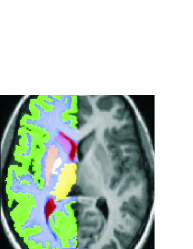
(a)

(b)

Figure 1: Left: An example registered brain image, overlaid by its accompanying anatomical labels, for cerebral white matter, cerebral cortex, lateral ventricle, thalamus, thalamus proper, caudate, and putamen. Labels are also divided into left and right, one side only shown here. Center: The bounding circle (green), the warp control points (red), and control point displacements (yellow), scaled to show relative not absolute magnitude. Right: The resultant warped image, which has a mean displacement of $d=3.0$ pixels.

IV-B Perturbing Ground Truth

We now considered perturbations about this found registration. Take $I_{i}$ as the $i^{th}$ registered 2D image, sampled at regular pixel positions $\{p_{a}:a=1,\ldots 141\times 141\}$. A warp of the image plane $\psi:\vec{p}\rightarrow\psi(\vec{p})$ produced a perturbed image function $\tilde{I}_{i}$, where $\tilde{I}_{i}(\psi(\vec{p}_{a}))\doteq I_{i}(\vec{p}_{a})$. The values $\{\tilde{I}_{i}(\psi(\vec{p}_{a}))\}$ were resampled back onto the regular pixel grid $\{\vec{p}_{a}\}$ using bilinear interpolation, to create the perturbed shape-free texture image $\{\tilde{I}_{i}(\vec{p}_{a}):a=1,\ldots 141\times 141\}$.

Our non-rigid image warps $\psi_{\mathrm{CPS}}$ were generated using the biharmonic clamped-plate spline (CPS, [28, 29]). The CPS has the boundary conditions that the warp is only non-zero in the interior of the unit circle. When applied to our square images, we take the boundary circle to be the inscribed circle (see Fig. 1b), with a set of initial knot-points positions arrayed within the circle. This means that we only deform this central region of the brain, and not the structure such as the skull. This makes the task of detecting the perturbations harder, in that misregistration of the strong tissue-edge features associated with the skull is much easier to detect than misregistrations of the more subtle structures within the brain.

To generate a warp with a specified mean pixel displacement $d$, each knot point was moved randomly, then the resultant mean pixel displacement $\hat{d}$ was calculated. Every pixel displacement was then scaled by the ratio $d/\hat{d}$, to give the exact required mean pixel displacement. The label images were warped along with the actual images.

IV-C Validation Results

We took a fixed subset of $N$ images from the set, and then applied multiple perturbations to this subset. For each instantiation of the perturbation, a value of $d$ was defined, and a random CPS warp of that size was generated for each image. We then computed the generalized Tanimoto overlap, and the specificity for the set of misaligned images. Various weightings were used within the generalized Tanimoto overlap, and we considered datasets of sizes $10<N\leq 50$. In Fig. 2, we show the case of $N=10$ images, subjected to various degrees of perturbation. We show the complexity-weighted Tanimoto overlap plotted against the specificity ($S_{\lambda}$ as in (4), with $M=50,000$ samples, and $\lambda=1$) of the shape-free texture model, for various values of the mean pixel displacement $d$.

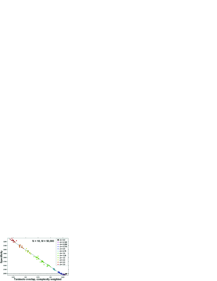
Figure 2: Specificity ($M=50,000$) plotted against complexity-weighted Tanimoto overlap, for perturbations of a set of $N=10$ images. The key shows the values of the mean displacement $d$. The dashed horizontal line shows the specificity for zero displacement, whereas the grey line shows the straight-line fit to the data for $d\geq 0.375$.

It can be seen that for values of $d\geq 0.375$ pixels, there is a very good linear relationship between the generalized Tanimoto overlap and the specificity. The maximum value of $d$ displayed is $d=3.0$, which as can be seen from Fig. 1b, is a large warp, but not a non-diffeomorphic one. Note that for a given value of the mean displacement $d$, there is some scatter of the points, as we might have expected given the random nature of the warp-generation process. The results are analogous when using other weightings, and other subset sizes.

TABLE II: The average size of each label, expressed as a percentage of the total labelled volume.

Label	Fractional Volume %
cerebral white matter	33.43
cerebral cortex	49.26
lateral ventricle	0.81
inferior lateral ventricle	0.05
cerebellum white matter	2.22
cerebellum cortex	8.33
thalamus proper	1.38
caudate	0.50
putamen	0.81
pallidum	0.28
$3^{rd}$ ventricle	0.07
$4^{th}$ ventricle	0.13
hippocampus	0.57
amygdala	0.29
brain stem	1.69
cerebrospinal fluid	0.10
accumbens area	0.08
left vessel	0.01

The dip in the specificity below the unperturbed value, for sub-pixel displacements $d\leq 0.375$, is a result of the image smoothing effect of such small displacements, a consequence of the necessary re-sampling and interpolation. This smoothing tends to move all images very slightly towards the mean image, and hence registers as a decrease in the specificity measure. As $d$ increases, the increases in the specificity measure from actual misalignment of structures competes with the smoothing effect. It is important to note that this problem at small displacements is not specific to this measure, and that any measure based on the distribution of the training set, and sensitive to the overall scale of the data set, will suffer from the same problem when evaluated using this perturbation method. Thus, apart from these unavoidable effects, we have shown that the specificity measure is strongly correlated with the ground truth overlap measure, as required.

V Assessing and Comparing Registration Algorithms

We now proceed to the reason for defining these measures, that is, to enable comparison of the performance of various non-rigid registration algorithms in cases where ground truth data is not available.

V-A Image Data

The image set to be registered was taken as the first 36 images from a dataset supplied by the Center for Morphometric Analysis (CMA) (as in [27]), consisting of T1-weighted 3D MR images of the brain. Images were acquired at different times with different scanners, and include control subjects, as well as subjects with Alzheimer’s disease, schizophrenia, attention deficit hyperactivity disorder, and prenatal drug exposure, with ages ranging from 4 years to 83 years. Manual annotations are available for 18 separate cortical and sub-cortical structures, and include both large-scale structures such as white-matter, cortex, and the ventricles, as well as more subtle structures such as the amygdala, thalamus, and caudate. A list is provided in Table II. This segmentation was performed at the CMA, using an extensively described semi-automated protocol [30, 31]. Although the number of images chosen for registration seems modest, it was sufficient to provide a realistic registration, and a good separation of the different registration algorithms in terms of label overlap.

V-B Registration Algorithms

Registration algorithms can be divided into two basic classes: pairwise (using only a pair of images) and groupwise.

V-B1 Pairwise & Repeated Pairwise

Given a pairwise algorithm, registration across a group of images can then be achieved by successive applications of the algorithm, which we will refer to as repeated pairwise, to make clear the distinction between this and inherently groupwise algorithms (e.g., [9]). All images in the group could each be pairwise-registered to some chosen reference example (e.g., [32]), but this suffers from the problem that, in general, the result obtained depends on the choice of reference. Refinements are possible, but the important point to note is that the correspondence for a single training image is defined w.r.t. this reference (which enables consistency of correspondence to be maintained across the group), and that the information used in determining the correct correspondence is limited to that contained in the single training set image and the single reference image. This approach explicitly does not take advantage of the full information in the group of images when defining correspondence [33]. Making better use of all the available information is the aim of groupwise registration algorithms, where correspondence is determined across the whole set in a principled manner.

A second important issue when constructing a registration algorithm is the way that the deformation fields are represented and manipulated. Fluid registration [34], with dense voxel-by-voxel flow over time, allows large-scale diffeomorphic deformations, but increases the computational complexity of the implementation. However, a fluid-based deformation field can capture subtleties of deformation not available to other methods. In contrast, a scheme such as piecewise-affine deformation fields allows a very compact representation of a deformation field, where the only variables are the positions and displacements of the nodes of the selected mesh. This compactness of the representation means that it is suitable for both pairwise and inherently groupwise registration algorithms. Such piecewise representations are also suitable for multi-resolution schemes, since the mesh can easily be sub-divided recursively.

Hence we take as our first registration algorithm a fluid-based approach, which performs repeated pairwise registration to a single reference image. The output was a set of dense 3D deformation fields defined at each voxel in each image.

The second and third registration algorithms chosen both used piecewise-affine deformation fields, and repeated-pairwise registration to a reference, differing only in their choice of reference image from the original dataset. These two references were selected, based on anecdotal evidence, as being close to or far from the mean of the set of images. The registration itself was realized as a coarse-to-fine process; a coarse body-centered cubic tetrahedral mesh was used to define a piecewise affine deformation field [35] over each image in the set. The deformation fields were optimized in a number of stages, starting from an initial global alignment achieved with a three-dimensional affine transformation. In subsequent stages, the density of the mesh was increased, and locations of individual mesh points were progressively optimized to match finer-scale details between each image and the reference. The process used a sum of absolute image differences as the objective function, and resulted in a set of optimized landmarks whose locations defined the final groupwise correspondence across all the images in the set.

V-B2 Groupwise

The fourth method considered was a groupwise registration approach, in which a combined reference to which each image is registered is evolved during the process. In this case, the reference was constructed as the mean image of the registered set. The reference hence starts blurred due to initial mis-alignment, but this allows a smooth optimization of deformation fields, the reference image then sharpening as the set is progressively brought into finer-scale alignment. The objective function for the registration is taken to be the sum of absolute differences between image voxels. In order to eliminate the effects of resolution, and due to time considerations and the desire to focus on the evaluation of the broad groupwise approach, we used an equivalent piecewise affine deformation field representation and optimization approach to that used in the pairwise cases. A full description of the algorithm can be found in Cootes et al. [36].

V-B3 Affine

Finally, an affine-only registration (that used as initialization for the piecewise-affine approaches) was included as the fifth method, as a control.

It is important to note that what matters are not the exact details of the methods of registration, but that we have applied five different registration methods to the same dataset, and that (apart from affine-only) each of these can be considered as a reasonable registration method that might be used in practise.

V-C Ground Truth Label Data and Registration Evaluation

Ground truth labels encompass the 18 types as detailed in Table II, and these are not divided into left and right for this experiment. In order to compute the Tanimoto overlap for the registered images and compare the different registration algorithms, the label images need to be warped, and the overlaps computed in a common spatial reference, as will be detailed in the next section. More important is the choice of label-weighting [16] to be used in the computation of the generalized Tanimoto overlap. In Table II, we show the relative volume of each of the 18 labels. It can be seen that structures such as the cerebral cortex and cerebral white matter account for over $80\%$ of the volume, with other important structures having less than $1\%$ of the total volume, with a range of volumes for the individual structures that encompasses three orders of magnitude. Hence if we used the simplest choice, of implicit-volume-weighting we can see that our evaluation of registration would be dominated by the registration results achieved on the cerebral cortex and cerebral white matter.

Hence we instead choose to use inverse-volume weighting, where the weight for a given label varies as the inverse of the label volume. This means that in the final measure, when summed over pixels, each of the labels will carry equal weight, whatever the size of the individual structure. This choice does not give undue prominence to any of the labels chosen for inclusion in the annotation. We also consider the case of simultaneous inverse-volume weighting and complexity weighting, to investigate whether in this case including complexity has any significant effect on our results. See [16] for further details.

V-D Building Models and Measuring Specificity

TABLE III: Generalized Tanimoto overlap and specificity, measured for the various registration algorithms shown. The generalized Tanimoto overlap is presented for two choices of the weighting, inverse-volume weighted, and inverse-volume weighted combined with a complexity weighting. Ranking results are presented in terms of rank order, and quantitative relative rank.

	Tanimoto Overlap						Specificity
	Inverse Volume			Inverse Volume & Complexity
Registration Algorithm	Score	Rank		Score	Rank		Score	Standard error	Rank
Fluid	0.611	1	100.0%	0.608	1	100.0%	0.131	0.0004	1	100.0%
Groupwise	0.564	2	83.0%	0.527	2	73.6%	0.162	0.0005	2	86.8%
Pairwise 1	0.546	4	76.4%	0.515	3	69.7%	0.173	0.0006	3	82.2%
Pairwise 2	0.553	3	79.0%	0.515	3	69.7%	0.174	0.0005	4	81.8%
Affine	0.335	5	0.0%	0.301	5	0.0%	0.367	0.0010	5	0.0%

For a given set of registered images, both the specificity (comparing registered training set images), and the generalized Tanimoto overlap (comparing registered label images) have to be evaluated in a common spatial reference frame. However, when it comes to comparing different registrations, it should be noted that in general, the spatial reference frame of one registration algorithm need not be the same as the spatial reference frame of another registration algorithm.

In order for a comparison of registration methods to be meaningful, we need to map the results of all registration methods into a single, common spatial reference frame. For the non-fluid registration methods, correspondence is defined via a set of mappings from the particular spatial reference frame to the frame of each original training set image. Whereas in the fluid case, correspondence is defined indirectly, via a dense mapping from each individual training image into the fluid reference frame. Hence when casting all results into a common reference, we use the fluid spatial reference, since it is straightforward to compose the mapping from the non-fluid spatial reference to the training image with the fluid mapping from the training image to the fluid spatial reference. Hence we obtain, for each registration algorithm, a registered set of training images (the shape-free texture images) $\mathcal{X}$, and a registered set of label images. The generalized Tanimoto overlaps can then be computed.

In order to compute the specificity for each algorithm, we first need to construct the shape-free texture model for that set of registered images. Since the spatial frame is common, we can use the same set of texture sample positions for each registration algorithm. The shape-free texture model is then constructed using standard PCA, where we retain all 35 non-normalized texture parameters/modes of variation in each case.

The sample set $\mathcal{Y}$ for each model is then generated as a set of $M=500000$ points in the space of non-normalized model parameters, distributed according to the distribution of the data $\mathcal{X}$. The Voronoi cell and distance computations for the specificity (6) are then performed in the space of parameters. We first compute the distances between every sample point and every training point, to extract the required nearest training example to each sample point. Note that in this case, rather than the $L_{2}$ Euclidean distance in parameter space (equivalent to the Euclidean distance in the space of images), we instead use the $L_{1}$ sum of absolute differences in parameter space. Although this $L_{1}$ distance is not rotationally symmetric, the parameters/axis system used respects the distribution of the training data, and hence justifies its use.

V-E Results

Table III gives the results for the specificity and generalized Tanimoto overlap, for all five methods of registration.

From the rank order results, it can be seen that all measures agree that the fluid method is best, followed by groupwise, pairwise, and finally affine; the only disagreement is in terms of the exact positioning of the two pairwise methods. In terms of the quantitative relative ranking (taking the score for the best method as $100\%$ and the score for the worst as $0\%$, and linear scaling between these two extremes), we can see that inverse-volume weighted generalized Tanimoto overlap is in rough agreement with the specificity results, with groupwise ranking $>83\%$, and both pairwise results $\approx 80\%$, with $\approx 4\%$ difference between groupwise and the best of the pairwise. The generalized Tanimoto overlap evaluated with combined inverse-volume and complexity weighting gives lowered relative ranking for groupwise and pairwise, but with still $\approx 4\%$ difference between groupwise and the best of the pairwise. This is perhaps to be expected; the addition of the complexity weighting gives more weight to labels with convoluted boundaries, and the fluid registration is better able to match such boundaries than the representation of deformation fields used in the groupwise and pairwise cases. The affine registration does badly in both cases. Hence the generalized Tanimoto overlap in the fluid case sees little change when the complexity weighting is included, whereas the groupwise and pairwise cases suffer a relative degradation in measured performance, as is shown by the relative rankings.

VI Discussion and Conclusions

We have described a model-based approach to assessing the accuracy of non-rigid registration of groups of images. The most important thing about this method is that it does not require any ground truth data, but depends only on the training data itself. A second important consideration is that the use of registered sets of images allows us to map the problem from the high-dimensional space of images, to the lower-dimensional space of PCA parameters (whether or not a linear model is then used at the next stage of actual modelling). This dimensionality-reduction means that the key figure is the number of examples, not their dimensionality, which makes the evaluation of 3D image registration much more practical.

For specificity, extensive validation experiments were conducted, based on perturbing correspondence obtained through registration. These show that our method is able to detect increasing misregistration using just the registered image data.

More importantly, we have shown that what is being measured by our model-based approach varies monotonically with an overlap measure based on ground truth, for the case of 2D slices extracted from 3D-registered brain data. Note that it is not essential in this case that the misregistration is biologically feasible, since we are not trying to recover the deformation itself, but instead compare the ground-truth based and model-based measures under misregistration.

Finally, we have applied our model-based measure to assessing the quality of various registration algorithms when applied to 3D MR brain images. This shows agreement, in terms of both the rank order and quantitative relative-ranking, between our method and ground truth based methods of evaluation.

It should be noted that the results presented here for the relative ranking of the registration algorithms considered are in general agreement with results presented elsewhere [6, 7], for extensive ground truth based evaluation of multiple registration algorithms on brain images. In particular, in Klein et al. (2010) [7], the authors considered label-based evaluation of the volumetric registration of pairs of images, both with and without an intermediate template. They found that using a customized, average template, constructed from a group of images similar to the pair being registered, gave improved performance. This is in agreement with our ranking of our groupwise algorithm (registration to an evolving averaged reference image) compared to our pairwise algorithms (registration to a fixed, non-averaged reference image).

It was noted both by Hellier (2003) [37], and by Klein et al. (2009) [6], that there is a (modest) correlation between the number of degrees of freedom of the deformation and registration accuracy. These observations are in agreement with our results (given the observation above about the relative positioning of groupwise compared to pairwise based on choice of reference or template). That is, the fluid algorithm was ranked highest (largest number of degrees of freedom), followed by the closely-spaced groupwise and pairwise methods (the same mesh-based representation of deformation, with a moderate number of degrees of freedom), and with affine (very small number of degrees of freedom) a long way behind.

We here used linear modelling in our evaluation, but in principle, any generative model-building approach could be used. This method is, in principle, very general, and can be applied to the results of any registration algorithm, as long as the assignment of (anatomical) correspondence across the entire group of images is both possible and meaningful.

We have only considered the registration of images of a single modality, where we obtain a simple distribution of registered images in image space, clustered about the mean image. Let us consider briefly the case of multimodal registration. Suppose we have a group of images split between two modalities $M_{1}$ and $M_{2}$, where each modality contains similar anatomical or structural information. We could then either register the entire set using, for example, mutual information as an image similarity measure, or we could register all the $M_{1}$ images, and all the $M_{2}$ images separately. Either way (provided we make a link between the two different spatial frames of the two means in the latter case), we then obtain a distribution of registered images in image space that will correspond to a cluster of registered images for each modality. The obvious next step is to model this distribution of all the images as a gaussian mixture model, allowing us to compute the specificity of the entire set. The two different registration scenarios presented above could then be compared. There are obviously other cases of multimodal registration which can be brought within a similar framework, but further exploration of this important issue is beyond the scope of the present paper.

Our model-based method hence represents a significant advance as regards the important problem of evaluating non-rigid registration algorithms. It establishes an entirely objective basis for evaluation, since it is free from the requirement of ground truth data. It also frees us from one caveat of label-based evaluation [6, 7], which is that such methods totally ignore misregistration within labelled regions.

References

- [1] F. P. Oliveira and J. M. R. Tavares, “Medical image registration: a review,” Computer Methods in Biomechanics and Biomedical Engineering, vol. 17, no. 2, pp. 73–93, 2014.
- [2] B. Zitová and J. Flusser, “Image registration methods: A survey,” Image and Vision Computing, vol. 21, pp. 977 – 1000, 2003.
- [3] P. Hellier, C. Barillot, I. Corouge, B. Gibaud, G. Le Goualher, D. L. Collins, A. Evans, G. Malandain, N. Ayache, G. E. Christensen, and H. J. Johnson, “Retrospective evaluation of intersubject brain registration,” IEEE Trans. Med. Imag., vol. 22, no. 9, pp. 1120–1130, 2003.
- [4] P. Rogelj, S. Kovacic, and J. C. Gee, “Validation of a nonrigid registration algorithm for multimodal data,” in Proceedings of Medical Imaging 2002, Image Processing, SPIE Proceedings, vol. 4684, 2002, pp. 299–307.
- [5] J. A. Schnabel, C. Tanner, A. C. Smith, M. O. Leach, C. Hayes, A. Degenhard, R. Hose, D. L. G. Hill, and D. J. Hawkes, “Validation of non-rigid registration using finite element methods,” in Information Processing in Medical Imaging (IPMI), ser. Lecture Notes in Computer Science, M. Insana and R. Leahy, Eds., vol. 2082. Springer, 2001, pp. 344–357.
- [6] A. Klein, J. Andersson, B. A. Ardekani, J. Ashburner, B. Avants, M.-C. Chiang, G. E. Christensen, D. L. Collins, J. Gee, P. Hellier, J. H. Song, M. Jenkinson, C. Lepage, D. Rueckert, P. Thompson, T. Vercauteren, R. P. Woods, J. J. Mann, and R. V. Parsey, “Evaluation of 14 nonlinear deformation algorithms applied to human brain MRI registration,” NeuroImage, vol. 46, no. 3, pp. 786–802, 2009.
- [7] A. Klein, S. S. Ghosh, B. Avants, B. T. T. Yeo, B. Fischl, B. Ardekani, J. C. Gee, J. J. Mann, and R. V. Parsey, “Evaluation of volume-based and surface-based brain image registration methods,” NeuroImage, vol. 51, no. 1, pp. 214–220, 2010.
- [8] T. F. Cootes, G. J. Edwards, and C. J. Taylor, “Active appearance models,” IEEE Trans. Pattern Anal. Machine Intell., vol. 23, pp. 681–685, 2001.
- [9] C. J. Twining, T. F. Cootes, S. Marsland, V. Petrovic, R. Schestowitz, and C. J. Taylor, “A unified information-theoretic approach to groupwise non-rigid registration and model building.” in Proceedings of Information Processing in Medical Imaging (IPMI), ser. Lecture Notes in Computer Science, G. Christensen and M. Sonka, Eds., vol. 3565. Springer, 2005, pp. 1–14.
- [10] R. H. Davies, C. J. Twining, T. F. Cootes, J. C. Waterton, and C. J. Taylor, “A minimum description length approach to statistical shape modeling,” IEEE Trans. Med. Imag., vol. 21, no. 5, pp. 525–537, 2002.
- [11] J. Ashburner, M. Brudfors, K. Bronik, and Y. Balbastre, “An algorithm for learning shape and appearance models without annotations,” Medical Image Analysis, vol. 55, pp. 197–215, 2019.
- [12] I. Goodfellow, J. Pouget-Abadie, M. Mirza, B. Xu, D. Warde-Farley, S. Ozair, A. Courville, and Y. Bengio, “Generative adversarial nets,” in Advances in neural information processing systems, 2014, pp. 2672–2680.
- [13] P. Jaccard, “Étude comparative de la distribution florale dans une portion des Alpes et des Jura,” Bulletin de la Société Vaudoise des Sciences Naturelles, vol. 37, pp. 547–579, 1901.
- [14] T. T. Tanimoto, “An elementary mathematical theory of classification and prediction,” IBM Internal Report, 1958.
- [15] D. J. Rogers and T. T. Tanimoto, “A computer program for classifying plants,” Science, vol. 132, no. 3434, pp. 1115–1118, 1960.
- [16] W. R. Crum, O. Camara, and D. L. G. Hill, “Generalized overlap measures for evaluation and validation in medical image analysis,” IEEE Trans. Med. Imag., vol. 25, no. 11, pp. 1451–1461, 2006.
- [17] T. Cootes, G. Edwards, and C. Taylor, “Active appearance models,” in Proceedings of the European Conference on Computer Vision (ECCV), ser. Lecture Notes in Computer Science, H. Burkhardt and B. Neumann, Eds., vol. 1407. Springer, 1998, pp. 484–498.
- [18] G. J. Edwards, T. F. Cootes, and C. J. Taylor, “Face recognition using active appearance models,” in Proceedings of European Conference on Computer Vision (ECCV), ser. Lecture Notes in Computer Science, H. Burkhardt and B. Neumann, Eds., vol. 1407. Springer, 1998, pp. 581–595.
- [19] M. de Groot, N. Patel, R. Manavaki, R. L. Janiczek, M. Bergstrom, A. Östör, D. Gerlag, A. Roberts, M. J. Graves, Y. Karkera et al., “Quantifying disease activity in rheumatoid arthritis with the TSPO PET ligand 18 F-GE-180 and comparison with 18 F-FDG and DCE-MRI,” EJNMMI Research, vol. 9, no. 1, pp. 1–11, 2019.
- [20] C. J. F. Reyneke, M. Lüthi, V. Burdin, T. S. Douglas, T. Vetter, and T. E. Mutsvangwa, “Review of 2-D/3-D reconstruction using statistical shape and intensity models and X-Ray image synthesis: Toward a unified framework,” IEEE reviews in biomedical engineering, vol. 12, pp. 269–286, 2018.
- [21] R. Cheng, H. R. Roth, L. Lu, S. Wang, B. Turkbey, W. Gandler, E. S. McCreedy, H. K. Agarwal, P. Choyke, R. M. Summers et al., “Active appearance model and deep learning for more accurate prostate segmentation on MRI,” in Medical Imaging 2016: Image Processing, vol. 9784. International Society for Optics and Photonics, 2016, p. 97842I.
- [22] A. F. Frangi, D. Rueckert, J. A. Schnabel, and W. J. Niessen, “Automatic construction of multiple-object three-dimensional statistical shape models: application to cardiac modelling,” IEEE Trans. Med. Imag., vol. 21, pp. 1151–1166, 2002.
- [23] C. J. Twining and C. J. Taylor, “Specificity: A graph-based estimator of divergence,” IEEE Trans. Pattern Anal. Machine Intell., vol. 33, no. 12, pp. 2492–2505, 2011.
- [24] R. Davies, C. J. Twining, and C. J. Taylor, Statistical models of shape: optimisation and evaluation. Springer, 2008.
- [25] R. Schestowitz, C. J. Twining, T. Cootes, V. Petrovic, C. J. Taylor, and W. R. Crum, “Assessing the accuracy of non-rigid registration with and without ground truth,” in Proceedings of the IEEE International Symposium on Biomedical Imaging: From Nano to Macro, 2006, pp. 836–839.
- [26] L. Tu, M. Styner, J. Vicory, S. Elhabian, R. Wang, J. Hong, B. Paniagua, J. C. Prieto, D. Yang, R. Whitaker, and S. M. Pizer, “Skeletal shape correspondence through entropy,” IEEE Trans. Med. Imag., vol. 37, no. 1, pp. 1–11, 2018.
- [27] K. O. Babalola, T. F. Cootes, C. J. Twining, V. Petrovic, and C. Taylor, “3D brain segmentation using active appearance models and local regressors,” in Medical Image Computing and Computer-Assisted Intervention (MICCAI), ser. Lecture Notes in Computer Science, D. Metaxas, L. Axel, G. Fichtinger, and G. Székely, Eds., vol. 5241. Springer, 2008, pp. 401–408.
- [28] C. J. Twining and S. Marsland, “Constructing an atlas for the diffeomorphism group of a compact manifold with boundary, with application to the analysis of image registrations,” Journal of Computational and Applied Mathematics, vol. 222, no. 2, pp. 411–428, 2008.
- [29] S. Marsland and C. J. Twining, “Constructing diffeomorphic representations for the groupwise analysis of the nonrigid registrations of medical images,” IEEE Trans. Med. Imag., vol. 23, no. 8, pp. 1006–1020, 2004.
- [30] P. A. Filipek, C. Richelme, D. N. Kennedy, and V. S. Caviness Jr, “The young adult human brain: An MRI-based morphometric analysis,” Cerebral Cortex, vol. 4, pp. 344–360, 1994.
- [31] M. Nishida, N. Makris, D. N. Kennedy, M. Vangel, B. Fischl, K. S. Krishnamoorthy, V. S. Caviness, and P. E. Grant, “Detailed semiautomated MRI based morphometry of the neonatal brain: preliminary results,” NeuroImage, vol. 32, no. 3, pp. 1041–1049, 2006.
- [32] D. Rueckert, A. F. Frangi, and J. A. Schnabel, “Automatic construction of 3-D statistical deformation models of the brain using nonrigid registration,” IEEE Trans. Med. Imag., vol. 22, no. 8, pp. 1014–1025, 2003.
- [33] T. F. Cootes, S. Marsland, C. J. Twining, K. Smith, and C. J. Taylor, “Groupwise diffeomorphic non-rigid registration for automatic model building,” in Proceedings of European Conference on Computer Vision (ECCV), ser. Lecture Notes in Computer Science, T. Pajdla and J. Matas, Eds., vol. 3024. Springer, 2004, pp. 316–327.
- [34] G. E. Christensen, R. D. Rabbitt, and M. I. Miller, “Deformable templates using large deformation kinematics,” IEEE Trans. Image Processing, vol. 5, pp. 1435–47, 1996.
- [35] T. Cootes, C. Twining, V. Petrovic, R. Schestowitz, and C. Taylor, “Groupwise construction of appearance models using piece-wise affine deformations,” in Proceedings of the British Machine Vision Conference (BMVC), vol. 2, 2005, pp. 879–888.
- [36] T. F. Cootes, C. J. Twining, V. S. Petrović, K. O. Babalola, and C. J. Taylor, “Computing accurate correspondences across groups of images,” IEEE Trans. Pattern Anal. Machine Intell., vol. 32, no. 11, pp. 1994–2005, 2009.
- [37] P. Hellier, “Consistent intensity correction of MR images,” in Proceedings 2003 International Conference on Image Processing (ICIP) (Cat. No.03CH37429), vol. 1, 2003, pp. 1109–1112.