Physics Constrained Learning for Data-driven Inverse Modeling from Sparse Observations

Abstract

Deep neural networks (DNN) have been used to model nonlinear relations between physical quantities. Those DNNs are embedded in physical systems described by partial differential equations (PDE) and trained by minimizing a loss function that measures the discrepancy between predictions and observations in some chosen norm. This loss function often includes the PDE constraints as a penalty term when only sparse observations are available. As a result, the PDE is only satisfied approximately by the solution. However, the penalty term typically slows down the convergence of the optimizer for stiff problems. We present a new approach that trains the embedded DNNs while numerically satisfying the PDE constraints. We develop an algorithm that enables differentiating both explicit and implicit numerical solvers in reverse-mode automatic differentiation. This allows the gradients of the DNNs and the PDE solvers to be computed in a unified framework. We demonstrate that our approach enjoys faster convergence and better stability in relatively stiff problems compared to the penalty method. Our approach allows for the potential to solve and accelerate a wide range of data-driven inverse modeling, where the physical constraints are described by PDEs and need to be satisfied accurately.

1 Introduction

Models involving partial differential equations (PDE) are usually used for describing physical phenomena in science and engineering. Inverse problems [1] aim at calibrating unknown parameters in the models based on observations associated with the output of the models. In real-world inverse problems, the observed data are usually “sparse” because only part of the model outputs are observable. Examples of inverse modeling from sparse observations include learning subsurface properties from seismic data on the earth’s surface [2] and learning constitutive relations from surface deformations of 3D solid materials [3]. The mapping from partial observations to unknown parameters is usually indirect and hard to compute, and in some cases, the inverse problems are ill-conditioned [4]. Recently, neural networks have been applied to learn unknown relations in inverse modeling [5, 6, 7], which is a more challenging task since training the neural network requires differentiating both neural network and PDEs for extracting gradients.

Mathematically, we can formulate the inverse problem as a PDE-constrained optimization problem

$$\min_{\theta}\ L(u)=\sum_{i\in\mathcal{I}_{\mathrm{obs}}}\left(u(\mathbf{x}_{i})-u_{i}\right)^{2}$$ (1)

$$\mathrm{s.t.}\;\;F(\theta,u)=0$$

where $L$ is the loss function that measures the discrepancy between estimated outputs $u$ and observed outputs $u_{i}$ at locations $\{\mathbf{x}_{i}\}$. $\mathcal{I}_{\mathrm{obs}}$ is the set of indices of locations where observations are available. $F$ is the physical constraint, usually described by a system of PDEs, and $\theta$ is the finite or infinite dimensional unknown parameter. In the case that $\theta$ is infinite dimensional, e.g., the unknown is a function, we can approximately represent the function with a functional form such as linear combination of basis functions or a neural network, in which case $\theta$ can be interpreted as coefficients of the functional form because there is a one-to-one correspondence between the function and its coefficients. For example, the constraint may have the form

$$F(\theta(u),u)=0$$

where $\theta(u)$ is a function that maps $u$ to a scalar or vector value. We use a neural network to approximate unknown functions, and we interpret $\theta$ as weights and biases in the neural network.

The physical constraints $F(\theta,u)=0$ is usually solved with numerical schemes. Let the discretization scheme be $F_{h}(\theta,u_{h})=0$ where $u_{h}$ is the numerical solution. We assume that the gradients $\frac{\partial F_{h}}{\partial\theta}$ and $\frac{\partial F_{h}}{\partial u_{h}}$ exist and are continuous, which is usually the case for PDE systems. For example, in the finite difference method for numerically solving PDE constraints $F(\theta,u)=0$, the gradients can be computed with adjoint state methods [8, 9, 10, 11, 12]. In the context of Eq. 1, the sparse observations $\{u_{i}\}_{i\in\mathcal{I}_{\mathrm{obs}}}$ are usually given as point values; therefore it is most appropriate to work with a strong form partial differential equation where we can read out function values $u(\mathbf{x}_{i})$ directly from numerical solutions to $F_{h}(\theta,u_{h})=0$ (in weak form, point-wise values are not defined). Additionally, to compute and store the Jacobian efficiently (used for solving the nonlinear PDEs), we assume that the basis functions in the numerical scheme are local, so that the Jacobian is sparse. Many standard numerical schemes, such as finite difference methods [13, 14] and iso-geometric analysis [15, 16], deal with strong form of PDEs and the discretization scheme is local.

The notion of sparse observations is not only important in practice but also has implications for computational methods. For example, if given full solution $u_{\mathrm{full}}$, we can estimate $\theta$ by minimizing the residual

$$\min_{\theta}\|F_{h}(\theta,u_{\mathrm{full}})\|_{2}^{2}$$

This is not possible for sparse observations; instead, we must solve for $u_{h}$ from $F_{h}(\theta,u_{h})=0$ and then compare $u_{h}$ with observations at locations $\{\mathbf{x}_{i}\}_{i\in\mathcal{I}_{\mathrm{obs}}}$.

One popular approach for solving Eq. 1 is by weakly enforcing the physical constraints by adding a penalty term to the discretized equations [17]

$$\tilde{L}_{h}(\theta,u_{h})=L_{h}(u_{h})+\lambda\|F_{h}(\theta,u_{h})\|_{2}^{2}$$ (2)

In this method, both $\theta$ and $u_{h}$ become independent variables in the unconstrained optimization. The gradients $\frac{\partial\tilde{L}_{h}(\theta,u_{h})}{\partial\theta}$ and $\frac{\partial\tilde{L}_{h}(\theta,u_{h})}{\partial u_{h}}$ can be computed using an adjoint approach, or automatic differentiation [18, 19, 20, 21, 22, 23]. The gradients are provided to a gradient-based optimization algorithm for minimizing Eq. 2. The physics-informed neural network (PINN) [24, 25, 26, 7] is an example where the penalty method can be applied. The penalty method is attractive since it avoids solving $F_{h}(\theta,u_{h})=0$ but the drawback is that the physical constraints are not satisfied exactly, and the number of optimization variables increases by including $u_{h}$ (either the discretized values or coefficients in the surrogate models). The number of extra degrees of freedom can be very large for dynamical problems, in which case $u_{h}$ is a collection of all solution vectors at each time step.

Another approach is to enforce the physical constraint by numerically solving the equation $F_{h}(\theta,u_{h})=0$ [27, 28, 29]. The solution $u_{h}(\mathbf{x};\theta)$ depends on $\theta$ and the objective function becomes

$$\tilde{L}_{h}(\theta)=L_{h}(u_{h}(\mathbf{x};\theta))$$

The optimal $\theta$ can be found using the gradient function

$$\nabla_{\theta}L_{h}(u_{h}(\mathbf{x};\theta))$$ (3)

The challenge is solving the equation $F_{h}(\theta,u_{h})=0$ and computing Eq. 3. If $F_{h}(\theta,u_{h})$ is nonlinear in $u_{h}$, we need the Jacobian $\frac{\partial F_{h}}{\partial u_{h}}$ in the Newton-Raphson method [30]. For computing Eq. 3, the finite difference method has been applied to this kind of problem but suffers from the curse of dimensionality and stability issues [31, 13]. Adjoint methods [8] can be used but can be time-consuming and error-prone to derive and implement.

We propose physics constrained learning (PCL) that enforces the physical constraint by solving $F_{h}(\theta,u_{h})=0$ numerically and uses reverse mode automatic differentiation and forward Jacobian propagation to extract the gradients and Jacobian matrices. The key is computing the gradient of the coupled system of neural networks and numerical schemes efficiently. It is worth mentioning that we optimize the storage and computational cost of Jacobian matrices calculation by leveraging their sparsity. However, if the solution representation is nonlocal, such as that in PINNs, the corresponding Jacobian matrices are dense, and thus enforcing physical constraints by solving the PDE system is challenging.

Our major finding is that compared to the penalty method, the convergence of PCL is potentially more robust and faster due to fewer iterations for stiff problems, despite each iteration being more expensive. Additionally, PCL does not require selecting a penalty parameter and therefore requires less effort to choose hyper-parameters. The PCL also simplifies the implementation by calculating gradients and Jacobians automatically using the reverse mode automatic differentiation and forward Jacobian propagation techniques. By formulating the observations and loss function $L(u)$ in terms of weak solutions (i.e., an integral of the product of the weak solution and a test function), the PCL can be generalized to numerical schemes that deal with weak form solutions such as finite element analysis. Therefore, the PCL promises to benefit a wide variety of inverse modeling problems.

We consider several applications of PCL for physics-based machine learning. We compare PCL with the penalty method, and we demonstrate that, in our benchmark problems,

1. PCL enjoys faster convergence with respect to the number of iterations to converge to a predetermined accuracy. Particularly, we observe a $10^{4}$ times speed-up compared with the penalty method in the Helmholtz problem. We also prove a convergence result, which shows that for the chosen model problem, the condition number in the penalty method is much worse than that of PCL.

2. PCL exhibits mesh independent convergence, while the penalty method does not scale with respect to the number of iterations as well as PCL when we refine the mesh.

3. PCL is more robust to noise and neural network architectures. The penalty method includes the solution $u_{h}$ as independent variables to optimize, and the optimizer may converge to a nonphysical local minimum.

The outline of the paper is as follows: in Section 2, we formulate the discrete optimization problem and discuss two different approaches: penalty methods and constraint enforcement methods. In Section 3, we present numerical benchmarks and compare the penalty methods and PCL. Finally, in Section 4, we summarize our results and discuss the limitations of PCL.

2 Data-driven Inverse Modeling with Sparse Observations

2.1 Problem Formulation and Notation

When the inverse problem Eq. 1 is discretized, $u$ and the output of $F$ will be vectors. We use the notation $u_{h}$, $L_{h}$, $F_{h}$ to denote $u$, $L$, $F$ in the discretized problem. $L_{h}:\mathbb{R}^{n}\rightarrow\mathbb{R}$, $F_{h}:\mathbb{R}^{d}\times\mathbb{R}^{n}\rightarrow\mathbb{R}^{n}$ are continuously differentiable functions. The discretized problem can be stated as

$$\min_{\theta}\;L_{h}(u_{h})$$ (4)

$$\mathrm{s.t.}\;\;F_{h}(\theta,u_{h})=0$$

For example, if we observe values of $u(x)$, $\{u_{i}\}_{i\in\mathcal{I}_{\mathrm{obs}}}$, at location $\{\mathbf{x}_{i}\}$, we can formulate the loss function with least squares

$$L_{h}(u_{h})=\sum_{i\in\mathcal{I}_{\mathrm{obs}}}\left(u_{h}(\mathbf{x}_{i})-u_{i}\right)^{2}$$

$F_{h}(\theta,u_{h})$ is the residual in the discretized numerical scheme.

Example 1.

In finite element analysis, if the system is linear, we have

$$F_{h}(\theta,u_{h})=A(\theta)u_{h}-b$$

where $b$ is the external load vector and $A(\theta)$ is the stiffness matrix of finite element analysis, taking into account the boundary conditions.

2.2 Penalty Method

The penalty method (PM) incorporates the constraint $F_{h}(\theta,u_{h})=0$ into the system by penalizing the term with a suitable norm (e.g., 2-norm in this work). We consider the class of differentiable penalized loss function

$$\tilde{L}_{h,\lambda}(\theta,u_{h}):=L_{h}(u_{h})+\lambda\|F_{h}(\theta,u_{h})\|_{2}^{2}$$

where $\lambda\in(0,\infty)$. The term $\lambda$ is called the multiplier of the penalty method and is used to control to what extent the constraint is enforced. We will omit the subscript $\lambda$ when it is clear from the context.

In the penalty method, the constraint may not be satisfied exactly. However, if the value $\lambda$ is made suitably large, the penalty term $\lambda\|F_{h}(\theta,u_{h})\|_{2}^{2}$ will impose a large cost for violating the constraint. Hence the minimization of the penalized loss function will yield a solution with small value in the residual term $F_{h}(\theta,u_{h})$. However, a large $\lambda$ places less weight on the objective function $L_{h}(u_{h})$. A proper choice of $\lambda$ for a desirable trade-off is nontrivial in many cases.

The penalty method can be visualized in Figure 1-left, where $\theta$ and $u_{h}$ both serve as trainable parameters. In the gradient-based optimization algorithm discussed in the next section, the gradients are back-propagated from the loss function to both $\theta$ and $u_{h}$ separately.

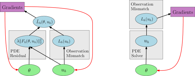
Figure 1: Schematic illustration of penalty method (left) and PCL (right).

The following theorem ensures that the penalty method converges to the optimal point under certain conditions

Theorem 2.1.

Assume that $L_{h}$ and $F_{h}$ are continuously differentiable functions, $\lambda\in(0,\infty)$ and the feasible set

$$S=\{u_{h}\in\mathbb{R}^{n}:F_{h}(\theta,u_{h})=0\}$$

is not empty. Assume $u^{k}$ is the global minimum of $\tilde{L}_{h,\lambda_{k}}(\theta,u_{h})$ at step $k$ of the algorithm, and $\lambda_{k}\to\infty$ as $k\rightarrow\infty$. Then the sequence $\{u^{k}\}$ converges to the solution of Eq. 4 as $k\rightarrow\infty$.

Proof.

See [32]. ∎

In practice, Theorem 2.1 may be of limited use since it requires solving a sequence of hard-to-solve unconstrained minimization problems. Still, under certain assumptions, it can provide an approximate solution of Eq. 4.

2.3 Physics Constrained Learning

We present an algorithm to compute the gradients of the loss function with respect to $\theta$ while numerically satisfying the physical constraint during optimization (Figure 1-right). We denote the numerical solution to $F_{h}(\theta,u_{h})=0$ by $u_{h}$, i.e.,

$$F_{h}(\theta,G_{h}(\theta))=0$$ (5)

The new loss function becomes

$$\tilde{L}_{h}(\theta)=L_{h}(G_{h}(\theta))$$

To derive the gradient $\frac{\partial\tilde{L}_{h}(\theta)}{\partial\theta}$, we apply the implicit function theorem to Eq. 5 and obtain

$$\frac{{\partial{F_{h}(\theta,u_{h})}}}{{\partial\theta}}+{\frac{{\partial{F_{h}(\theta,u_{h})}}}{{\partial{u_{h}}}}}\frac{\partial G_{h}(\theta)}{\partial\theta}=0\qquad\Rightarrow$$

$$\frac{\partial G_{h}(\theta)}{\partial\theta}=-\Big{(}\frac{{\partial{F_{h}(\theta,u_{h})}}}{{\partial{u_{h}}}}\Big{)}^{-1}\frac{{\partial{F_{h}(\theta,u_{h})}}}{{\partial\theta}}$$

Therefore we have

$$\frac{{\partial{{\tilde{L}}_{h}}(\theta)}}{{\partial\theta}} =\frac{\partial{{L}_{h}}(u_{h})}{\partial u_{h}}\frac{\partial G_{h}(\theta)}{\partial\theta}$$

$$=-\frac{{\partial{L_{h}}({u_{h}})}}{{\partial{u_{h}}}}\;\Big{(}{\frac{{\partial{F_{h}(\theta,u_{h})}}}{{\partial{u_{h}}}}\Big{|}_{u_{h}={G_{h}}(\theta)}}\Big{)}^{-1}\;\frac{{\partial{F_{h}(\theta,u_{h})}}}{{\partial\theta}}\Big{|}_{u_{h}={G_{h}}(\theta)}$$ (6)

Now we discuss how to compute Eq. 6 efficiently. Assume that the number of parameters in $\theta$ is $p$, the degrees of freedom of $u_{h}$ is $N$, the complexity of solving a linear system with coefficient matrix $\frac{\partial{F_{h}(\theta,u_{h})}}{\partial u_{h}}$ is $C$ (together with boundary conditions) and the complexity of evaluating $F_{h}(\theta,u_{h})$ is $C^{\prime}$. Additionally, in the following complexity estimation, we assume that we have already solved $F_{h}(\theta,u_{h})=0$ and obtain the solution vector $u_{h}$. There are in general two strategies to compute Eq. 6:

1. We compute Eq. 6 from right to left, i.e., compute

   $$z=\underbrace{\Big{(}{\frac{{\partial{F_{h}}}}{{\partial{u_{h}}}}\Big{|}_{u_{h}={G_{h}}(\theta)}}\Big{)}^{-1}}_{N\times N}\;\;\underbrace{\frac{{\partial{F_{h}}}}{{\partial\theta}}\Big{|}_{u_{h}={G_{h}}(\theta)}}_{N\times p}$$

   which has cost $\mathcal{O}(pC)$ and then compute

   $$\underbrace{\frac{{\partial{L_{h}}({u_{h}})}}{{\partial{u_{h}}}}}_{1\times N}\;z$$

   which has cost $\mathcal{O}(Np)$. The total cost is $\mathcal{O}(\max\{Np,pC\})=\mathcal{O}(pC)$ (typically $C$ is at least $\mathcal{O}(N)$).

2. We first compute

   $$w^{T}=\underbrace{\frac{{\partial{L_{h}}({u_{h}})}}{{\partial{u_{h}}}\rule[-9.0pt]{1.0pt}{0.0pt}}}_{1\times N}\;\;\underbrace{\Big{(}{\frac{{\partial{F_{h}}}}{{\partial{u_{h}}}}\Big{|}_{u_{h}={G_{h}}(\theta)}}\Big{)}^{-1}}_{N\times N}$$

   which is equivalent to solving a linear system

   $${\left({\frac{{\partial{F_{h}}}}{{\partial{u_{h}}}}\Bigg{|}_{u_{h}={G_{h}}(\theta)}}\right)^{T}}w=\left(\frac{{\partial{L_{h}}({u_{h}})}}{{\partial{u_{h}}}}\right)^{T}$$ (7)

   with cost $\mathcal{O}(C)$, and then compute (in the following operation, we assume $w$ is independent of $\theta$)

   $$w^{T}\;\underbrace{\frac{{\partial{F_{h}}}}{{\partial\theta}}\Big{|}_{u_{h}={G_{h}}(\theta)}}_{N\times p}=\frac{\partial(w^{T}\;{F_{h}}(\theta,u_{h}))}{\partial\theta}\Bigg{|}_{u_{h}={G_{h}}(\theta)}$$

   If we apply reverse mode automatic differentiation, using fused-multiply adds, denoted by OPS, as a metric of computational complexity, we have [33, 34]

   $$\mathrm{OPS}\left(\frac{\partial(w^{T}\;{F_{h}}(\theta,u_{h}))}{\partial\theta}\right)\leq 4\;\mathrm{OPS}({F_{h}}(\theta,u_{h})))$$ (8)

   Therefore, the total computational cost will be $\mathcal{O}(\max\{C^{\prime},C\})$.

In the case when $p$ is large, e.g., $p$ are the weights and biases of a neural network, the second approach is preferable. Hence, we adopt the second strategy in our implementation.

In many physical simulations, we need to solve a linear system, which can be expressed as

$$F_{h}(\theta_{1},\theta_{2},u_{h})=\theta_{1}-A(\theta_{2})u_{h}=0$$ (9)

Applying Eq. 6 to Eq. 9, we have

$$p :=\frac{\partial\tilde{L}_{h}(\theta_{1},\theta_{2})}{\partial\theta_{1}}=\frac{\partial L_{h}(u_{h})}{\partial u_{h}}A(\theta_{2})^{-1}$$

$$q :=\frac{\partial\tilde{L}_{h}(\theta_{1},\theta_{2})}{\partial\theta_{2}}=-\frac{\partial L_{h}(u_{h})}{\partial u_{h}}A(\theta_{2})^{-1}\frac{\partial A(\theta_{2})}{\partial\theta_{2}}$$

which is equivalent to

$$A^{T}p^{T}=\left(\frac{\partial L_{h}(u_{h})}{\partial u_{h}}\right)^{T}\quad q=-p\frac{\partial A(\theta_{2})}{\partial\theta_{2}}$$

In the following, we consider a concrete example of Eq. 9.

Example 2.

We consider the following example: solve an inverse modeling problem with the 1D Poisson equation, with $F(\theta,u)=0$ expressed as

$$\frac{\partial}{\partial x}\left(f(u(x);\theta)\;\frac{\partial u(x)}{\partial x}\right) =g(x) x\in(0,1)$$ (10)

$$u(0)=u(1) =0$$

where $f(u(x);\theta)$ is a function of $u(x)$ parametrized by an unknown parameter $\theta$. For example, $f(u(x);\theta)$ can be a neural network which maps $u(x)$ to a scalar value and $\theta$ are the weights and biases. The sparse observations are $u_{i,\mathrm{obs}}$, the true values of $u(x)$ at location $i\in\mathcal{I}_{\mathrm{obs}}$, and $\mathcal{I}_{\mathrm{obs}}\subset\mathbb{N}$ is a set of location index.

We apply the finite difference method to Eq. 10. We discretize $u$ on a uniform grid with interval length $h$ and node $x_{i}=\frac{i-1}{n}$, $i=1,2,\ldots,n+1$. $u_{i}$ denotes the discretized values at $x_{i}$, $u_{h}=[u_{1},u_{2},\ldots,u_{n+1}]$ and $g_{i}=g(x_{i})$. The corresponding $F_{h}(\theta,u_{h})$ is

$${F_{h}(\theta,u_{h})}_{i}=f\left(\frac{u_{i}+u_{i+1}}{2};\theta\right)\frac{u_{i+1}-u_{i}}{h^{2}}-f\left(\frac{u_{i}+u_{i-1}}{2};\theta\right)\frac{u_{i}-u_{i-1}}{h^{2}}-g_{i}$$

$$i=2,3,\ldots,n$$

$$u_{1}=u_{n+1}=0$$

Assume that the observations are located exactly at some of the grid nodes, the loss function can be formulated as

$$L_{h}(u_{h})=\sum_{i\in\mathcal{I}_{\mathrm{obs}}}\left(u_{i}-u_{i,\mathrm{obs}}\right)^{2}$$

and therefore, we have

$$\frac{{\partial{L_{h}}({u_{h,i}})}}{{\partial{u_{h}}}}=\begin{cases}2\left(u_{i}-u_{i,\mathrm{obs}}\right)&i\in\mathcal{I}_{\mathrm{obs}}\\ 0&i\not\in\mathcal{I}_{\mathrm{obs}}\end{cases}$$ (11)

The Jacobian of $F_{h}(\theta,u_{h})$ with respect to $u_{h}$ is

$$\frac{\partial{F_{h}(\theta,u_{h})}_{i}}{\partial u_{h,j}}=\ \frac{\partial}{\partial u}f\left(\frac{u_{i}+u_{i+1}}{2};\theta\right)\frac{\delta_{i,j}+\delta_{i+1,j}}{2}\frac{u_{i+1}-u_{i}}{h^{2}}$$

$$+f\left(\frac{u_{i}+u_{i+1}}{2};\theta\right)\frac{\delta_{i+1,j}-\delta_{i,j}}{h^{2}}$$

$$-\frac{\partial}{\partial u}f\left(\frac{u_{i}+u_{i-1}}{2};\theta\right)\frac{\delta_{i,j}+\delta_{i-1,j}}{2}\frac{u_{i}-u_{i-1}}{h^{2}}$$

$$-f\left(\frac{u_{i}+u_{i-1}}{2};\theta\right)\frac{\delta_{i,j}-\delta_{i-1,j}}{h^{2}}$$ (12)

where

$$\delta_{ij}=\begin{cases}1&i=j\\ 0&i\neq j\end{cases}$$

Note that for fixed $i$, $\frac{\partial{F_{h}(\theta,u_{h})}_{i}}{\partial u_{j}}$ can only be nonzero for $j=i-1,i,i+1$ and therefore the Jacobian matrix is sparse.

Additionally, we have

$$\begin{split}\frac{{\partial{F_{h}}}}{{\partial\theta}}(\theta,{G_{h}}(\theta))&=\nabla_{\theta}f\left(\frac{u_{i}+u_{i+1}}{2};\theta\right)\frac{u_{i+1}-u_{i}}{h^{2}}\\ &\hskip 40.00006pt-\nabla_{\theta}f\left(\frac{u_{i}+u_{i-1}}{2};\theta\right)\frac{u_{i}-u_{i-1}}{h^{2}}\end{split}$$ (13)

Using the results from Eqns. 11, 12 and 13 and the formula Eq. 6 we obtain the gradient ${{\partial{{\tilde{L}}_{h}}(\theta)}}/{{\partial\theta}}$.

Remark 1.

In practice, if the system of PDEs or the relation between $f(u;\theta)$ and $\theta$ is complex (e.g., a neural network), deriving and implementing Eqns. 12 and 13 are challenging. Fortunately, we can compute those terms using automatic differentiation techniques. We present the technical details in E and F.

2.4 Analysis of PCL

In the penalty method, the constraint $F(\theta,u)=0$ is imposed by including a penalty term $\|F_{h}(\theta,u_{h})\|^{2}_{2}$ in the loss function, and the summation of the penalty term and the observation error is minimized simultaneously with gradient descent methods. Intuitively, if the problem $F_{h}(\theta,u_{h})=0$ is stiff, the penalty method suffers from slow convergence due to worse condition number of the least square loss $\|F_{h}(\theta,u_{h})\|^{2}_{2}$ compared to the original problem $F_{h}(\theta,u_{h})=0$.

In this section, we analyze the convergence by considering a model problem

$$\min_{\theta}\|u-u_{0}\|^{2}_{2}$$

$$\text{s.t.}\;\;Au=\theta y$$

where $\theta\in\mathbb{R}$ is unknown and $A$ is a nonsingular square coefficient matrix. For simplicity, assume that the true value for $\theta$ is $1$, and $u_{0}=A^{-1}y$.

In PCL, we have

$$\tilde{L}_{h}(\theta)=\|\theta A^{-1}y-u_{0}\|^{2}_{2}=(\theta-1)^{2}\|u_{0}\|_{2}^{2}$$

which is a quadratic function in $\theta$ and can be minimized efficiently using gradient-based method. Nevertheless, we have to solve $Au=y$, and the computational cost usually depends on the condition number $\kappa(A)$.

In the penalty method, the new loss function is

$$\min_{\theta,u_{h}}\tilde{L}_{h}(\theta,u_{h})=\|u_{h}-u_{0}\|^{2}_{2}+\lambda\|Au_{h}-\theta y\|_{2}^{2}$$ (14)

Eq. 14 is equivalent to a least square problem $\min_{\bm{\theta}}\|\mathbf{A}\bm{\theta}-\mathbf{y}\|_{2}^{2}$ with the coefficient matrix and the right hand side

$$\mathbf{A}_{\lambda}=\begin{bmatrix}I&0\\ \sqrt{\lambda}A&-\sqrt{\lambda}y\end{bmatrix},\qquad\mathbf{y}=\begin{bmatrix}u_{0}\\ 0\end{bmatrix}$$

The least-square problem has a condition number that is at least $\kappa(A)^{2}$ asymptotically, which is implied by the following theorem:

Theorem 2.2.

The condition number of $\mathbf{A}_{\lambda}$ is

$$\liminf_{\lambda\rightarrow\infty}\kappa(\mathbf{A}_{\lambda})\geq\kappa(A)^{2}$$

and therefore, the condition number of the unconstrained optimization problem from the penalty method is the square of that from PCL asymptotically.

Proof.

Assume that the singular value decomposition of $A$ is

$$A=U\Sigma V^{T}$$

where

$$\Sigma=\mathrm{diag}(\sigma_{1},\sigma_{2},\ldots,\sigma_{n})$$

Without loss of generality, we assume $\sigma_{1}\geq\sigma_{2}\geq\cdots\geq\sigma_{n}>0$. We have

$$\mathbf{A}_{\lambda}=\lambda\begin{bmatrix}V&0\\ 0&1\end{bmatrix}\begin{bmatrix}\frac{1}{\lambda}I+\Sigma^{2}&\alpha\\ \alpha^{T}&s\end{bmatrix}\begin{bmatrix}V^{T}&0\\ 0&1\end{bmatrix}$$

for

$$s=y^{T}y,\qquad\alpha=-\Sigma U^{T}y$$

Note

$$B=\begin{bmatrix}\frac{1}{\lambda}I+\Sigma^{2}&\alpha\\ \alpha^{T}&s\end{bmatrix}$$

is an arrowhead matrix and its eigenvalues are expressed by the zeros of [35]

$$f(x)=s-x-\sum_{i=1}^{n}\frac{\alpha_{i}^{2}}{\sigma_{i}^{2}+\frac{1}{\lambda}-x}$$

Note that

$$\lim_{x\rightarrow\left(\sigma_{i}^{2}+\frac{1}{\lambda}\right)+}f(x)\rightarrow+\infty,\quad\lim_{x\rightarrow\left(\sigma_{i}^{2}+\frac{1}{\lambda}\right)-}f(x)\rightarrow-\infty$$

and

$$\lim_{x\rightarrow+\infty}f(x)=-\infty\quad\lim_{x\rightarrow-\infty}f(x)=+\infty$$

We infer that the $n+1$ eigenvalues of $B$ are located in $(0,\sigma_{1}^{2}+\frac{1}{\lambda})$, $(\sigma_{1}^{2}+\frac{1}{\lambda},\sigma_{2}^{2}+\frac{1}{\lambda})$, $\ldots$, $(\sigma_{n}^{2}+\frac{1}{\lambda},\infty)$. The smallest eigenvalue of $B$ is positive since $A$ is positive definite and so is $B$.

Therefore, we deduce that $\kappa(\mathbf{A}_{\lambda})\geq\frac{\sigma_{n}^{2}+\frac{1}{\lambda}}{\sigma_{1}^{2}+\frac{1}{\lambda}}$, thus

$$\liminf_{\lambda\rightarrow\infty}\kappa(\mathbf{A}_{\lambda})\geq\frac{\sigma_{n}^{2}}{\sigma_{1}^{2}}=\kappa(A)^{2}$$

∎

3 Numerical Benchmarks

In this section, we perform four numerical benchmarks and compare physics constrained learning (PCL) and the penalty method (PM). Unless specified, we use L-BFGS-B [32, 36] to minimize the loss function for both methods, and use the same tolerance $\varepsilon=10^{-12}$ for the gradient norm and the relative function change, i.e., we stop the iteration if

$$\|\nabla_{\theta}l(z)\|<\varepsilon\qquad\left|\frac{l(z)-l(z^{\prime})}{l(z^{\prime})}\right|<\varepsilon$$

where $z$ and $z^{\prime}$ represent the candidate parameter at the current and previous step and

PCL: $$z =\theta, l(z) =\tilde{L}_{h}(\theta)$$

PM: $$z =(\theta,u_{h}), l(z) =\tilde{L}_{h}(\theta,u_{h})$$

To show that PCL is applicable for various numerical schemes and PDEs, we test various PDEs, numerical schemes and inverse problem types, which are listed in Table 1.

Example	PDE	Numerical Scheme	Unknown Type
1	Linear Static	IGA	Parameter
2	Nonlinear Static	FD	Function
3	Nonlinear Dynamic	FVM	Function

Table 1: Numerical Benchmarks. IGA is short for the isogeometric analysis; FD is short for the finite difference method. FVM is short for the finite volume method. When the unknown type is a function, we use a deep neural network to approximate the unknown function and couple it with numerical schemes.

3.1 Parametric Inverse Problem: Helmholtz Equation

We consider the inverse problem for a Helmholtz equation [37, 38, 39]. Let $\Omega$ be a bounded domain in 2D, and the Helmholtz equation is given by

$$\Delta u+k^{2}g(\mathbf{x})u=0$$ (15)

with the Dirichlet boundary condition

$$u(\mathbf{x})=u_{0}(\mathbf{x}),\ \mathbf{x}\in\partial\Omega$$ (16)

where $u(\mathbf{x})$ denotes the electric field, the amplitude of a time-harmonic wave, or orbitals for an energy state depending on the models. The parameter $k$ is the frequency and $g(\mathbf{x})$ is a physical parameter. In the applications, we want to recover $g(\mathbf{x})$ based on boundary measurements, i.e., the values of $u(\mathbf{x})$ and $h(\mathbf{x})=\frac{\partial u}{\partial n}(\mathbf{x})$. $g(\mathbf{x})$ are given in a parametric form

$$g(\mathbf{x})=ax^{2}+bxy+cy^{2}+dx+ey+f,\ \mathbf{x}=(x,y)$$

where $\theta=(a,b,c,d,e,f)$ are unknown parameters.

Assume we have observed $h_{i}$, i.e., the values of $\frac{\partial u}{\partial n}(\mathbf{x})$ on the boundary points $\{\mathbf{x}_{i}\}_{i\in\mathcal{I}_{\mathrm{obs}}}$, the optimization problem can be formulated as

$$\min_{\theta}\ L(u)=\frac{1}{n_{\mathrm{obs}}}\sum_{i\in\mathcal{I}_{\mathrm{obs}}}\left(\frac{\partial u}{\partial n}(\mathbf{x}_{i})-h_{i}\right)^{2}$$ (17)

$$\mathrm{s.t.}\;\;F_{h}(\theta,u_{h})=0$$

Here $F_{h}(\theta,u_{h})=0$ is the IGA discretization of Eq. 15 with the boundary condition Eq. 16.

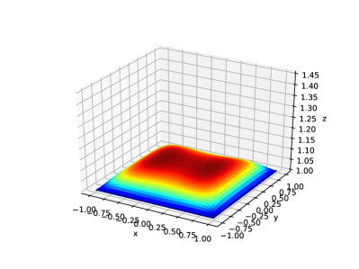
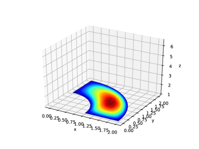
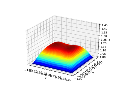
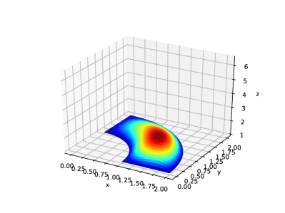
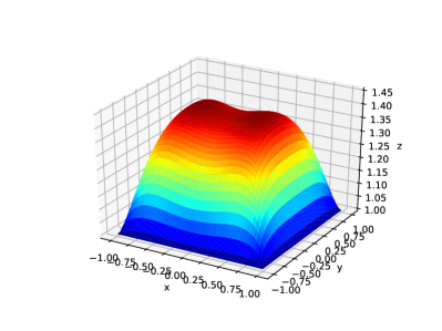
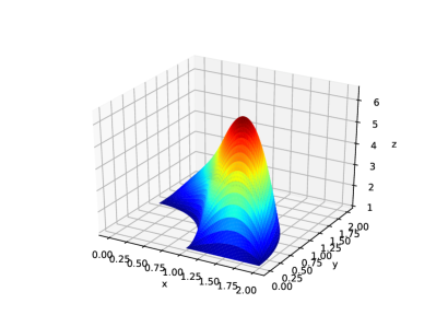
Figure 2: Solution profiles of Eq. 15 for a square domain and a quarter of annulus domain. The three rows correspond to $k=0.5$, $k=0.75$ and $k=1.0$.

For verification, we use the parameters $\theta^{*}=(5,0,2,0,0,0)$, i.e.,

$$g(\mathbf{x})=5x^{2}+2y^{2}$$

The boundary condition is given by $u_{0}(\mathbf{x})\equiv 1$. We consider a square domain and a quarter of an annulus domain. The solution profiles are shown in Figure 2 for different $k$. The error of the inverse modeling problem is measured by

$$\mathrm{error}=\|\theta-\theta^{*}\|_{2}$$

where $\theta$ is the estimated parameter by solving Eq. 17.

(a) Square domain, refinement level = 5.

(b) Square domain, refinement level = 6.

Figure 3: Convergence comparison of PM and PCL for the square domain. Note that the scale of “Iterations” are different. Here “refinement” denotes the number of mesh refinement processes from the initial domain in the isogeometric analysis discretization. Each refinement process adds an extra knot between two knots in the original knot vector in each dimension.

(a) Pipe domain, refinement level = 5.

(b) Pipe domain, refinement level = 6.

Figure 4: Convergence comparison of PM and PCL for the curved pipe domain.

We apply both PM and PCL to this problem. The PCL method exhibits a dramatic acceleration of convergence in terms of the number of iterations. PCL can achieve the same accuracy, such as $10^{-3}$ with only a few iterations, compared with more than $10^{4}$ iterations for PM. Moreover, PCL can achieve better accuracy than PM, as demonstrated the error in Figures 3 and 4.

PCL is also more scalable to mesh sizes. We apply $h$-refinement to the meshes in Figures 3 and 4. We see that the PM method requires more iterations to converge to the same accuracy. The number of iterations in the PCL method is less sensitive to the mesh sizes, although a larger sparse linear system is solved per iteration. Another observation is that PCL converges faster for smaller frequencies. However, PM does not exhibit such properties in our test cases.

3.2 Physics Based Machine Learning: Static Problem

In this example, we consider the equation

$$-\nabla\cdot(\mathbf{f}(u)\nabla u)= \;h(\mathbf{x}) \mbox{ in }\Omega$$ (18)

$$u= \;u_{0}(\mathbf{x}) \mbox{ on }\partial\Omega$$

where $\Omega=[0,1]^{2}$. We assume that $\mathbf{f}(u)\in\mathbb{R}^{2\times 2}$ and has the form

$$\mathbf{f}(u)=\begin{bmatrix}f_{1}(u)&0\\ 0&f_{2}(u)\end{bmatrix}$$

Figure 5: Test function sets. Note in test function set 4, $f_{2}(u)$ does not have continuous derivatives at $u=0.3$.

We test four sets of $\mathbf{f}(u)$ (Figure 5)

1. Test Function Set 1

   $$f_{1}(u)=0.1+u^{3.1},\qquad f_{2}(u)=0.1+u^{3.5}$$

2. Test Function Set 2

   $$f_{1}(u)=0.1+0.1\cos(u),\qquad f_{2}(u)=0.1+0.1\sin(u)$$

3. Test Function Set 3

   $$f_{1}(u)=0.1+u^{3},\qquad f_{2}(u)=0.1+\frac{0.1}{1+u^{2}}$$

4. Test Function Set 4

   $$f_{1}(u)=0.1+u^{2},\qquad f_{2}(u)=0.1+\max(0,u-0.3)$$

We use a deep neural network to approximate $\mathbf{f}$, which takes $u$ as input and outputs $f_{1}(u;\theta)$ and $f_{2}(u;\theta)$ ($\theta$ is the weights and biases)

$$\mathbf{f}_{\theta}(u)=\begin{bmatrix}f_{1}(u;\theta)&0\\ 0&f_{2}(u;\theta)\end{bmatrix}$$

The neural network is a $k$ hidden layer (we test multiple options: $k=1$, …, $5$) and has 20 neurons per layer and tanh activation functions since it is continuously differentiable and bounded so it does not create extreme values in the intermediate layers.

The full solution on the grid is solved numerically and used as an observation, but the codes developed for this problem also work for sparse solutions. For PCL, we discretize Eq. 18 with the finite difference method on a $31\times 31$ uniform grid. We demonstrate that even with this simple fully-connected architecture, the neural network can learn $\mathbf{f}(u)$ reasonably well. We compare PCL with PM; we vary the neural network architectures (different hidden layers) and penalty parameters $\lambda$ for PM, which we denote PM-$\lambda$. The error is reported by

$$\sqrt{\sum_{i=1}^{N+1}(f_{1}(u_{i})-f_{1}(u_{i};\theta))^{2}+\sum_{i=1}^{N+1}(f_{2}(u_{i})-f_{2}(u_{i};\theta))^{2}}$$

where $f_{1}(u;\theta)$ and $f_{2}(u;\theta)$ are the first and second outputs of the neural network with parameter $\theta$. $u_{i}=0.6\frac{i-1}{N}$ for $i=1,2,\ldots,N+1$ ($N=99$ in our case); we choose $0.6$ since $[0,0.6]$ is the region where the solution $u$ is. We run the experiments for sufficiently long time so that the parameters nearly converge to a local minimum.

Tables 2, 3, 4 and 5 show the error for the four test function sets. Additionally, we show the relative error for each $u$ in Figure 6 for PCL and PM-0.01. We can see that PCL outperforms PM in almost all cases, regardless of the neural network architectures. PM performs better than PCL only in a few cases, such as in the test function set 1 with $\lambda=0.01$ and $\lambda=1$ and the test function set 3 with $\lambda=0.01$; for other $\lambda$ and neural network architectures, PM fails to converge to the true functions. The sensitivity to the neural network hyperparameters and penalty parameters can be a difficulty when applying the penalty method. PM introduces more dependent variables for optimization, and, therefore, it is likely that the optimizer converges to a local minimum that is nonphysical. Note that the accuracy does not necessarily improve as we increase the number of hidden layers because larger neural networks are harder to optimize.

Method\Hidden Layers	1	2	3	4	5
PCL	$1.6\times 10^{-2}$	$1.1\times 10^{-2}$	$2.7\times 10^{-2}$	$4.5\times 10^{-2}$	$3.5\times 10^{-2}$
PM-0.0	1.7	$9.7\times 10^{-1}$	$7.8\times 10^{-1}$	$1.9\times 10^{-3}$	2.8
PM-0.1	7.2	5.3	3.7	8.8	2.1
PM-1	1.8	5.2	2.9	$4.2\times 10^{-3}$	1.7
PM-10	7.4	2.8	1.9	4.7	1.8
PM-100	2.1	2.6	3.0	3.9	2.6

Table 2: Error for test function set 1.

Method\Hidden Layers	1	2	3	4	5
PCL	$4.1\times 10^{-5}$	$2.4\times 10^{-4}$	$6.8\times 10^{-4}$	$1.1\times 10^{-3}$	$3.8\times 10^{-3}$
PM-0.0	$8.0\times 10^{-1}$	1.5	$9.3\times 10^{-1}$	$1.9\times 10^{-3}$	4.9
PM-0.1	3.8	1.9	$1.1\times 10^{1}$	6.7	1.6
PM-1	2.3	$2.8\times 10^{-3}$	$2.4\times 10^{1}$	2.7	2.7
PM-10	3.2	2.7	$1.6\times 10^{-2}$	2.6	2.9
PM-100	3.2	2.1	2.6	2.5	2.8

Table 3: Error for test function set 2.

Method\Hidden Layers	1	2	3	4	5
PCL	$8.7\times 10^{-3}$	$3.0\times 10^{-2}$	$2.9\times 10^{-2}$	$3.4\times 10^{-2}$	$5.4\times 10^{-2}$
PM-0.0	8.0	5.6	4.5	$1.1\times 10^{-2}$	1.0
PM-0.1	5.3	$3.8\times 10^{1}$	8.0	6.4	7.2
PM-1	$1.9\times 10^{1}$	$3.0\times 10^{-2}$	4.3	$2.0\times 10^{1}$	2.3
PM-10	3.6	4.4	$2.7\times 10^{-2}$	$1.1\times 10^{1}$	4.6
PM-100	1.6	5.3	4.2	$8.9\times 10^{-2}$	4.4

Table 4: Error for test function set 3.

Method\Hidden Layers	1	2	3	4	5
PCL	$3.1\times 10^{-1}$	$8.4\times 10^{-1}$	$2.3\times 10^{-1}$	$1.2\times 10^{-1}$	$1.4\times 10^{-1}$
PM-0.0	$2.1\times 10^{-1}$	4.8	$7.3\times 10^{-1}$	2.5	4.1
PM-0.1	3.7	$2.0\times 10^{1}$	7.2	4.8	5.4
PM-1	4.3	$1.7\times 10^{1}$	3.2	5.9	4.3
PM-10	4.4	3.3	7.1	2.3	9.7
PM-100	3.1	$8.2\times 10^{-1}$	3.1	3.8	3.1

Table 5: Error for test function set 4.

                          

Figure 6: The relative error for PCL and PM-0.01 for different test function sets.

3.3 Physics Based Machine Learning: Time-Dependent PDEs

Finally, we consider the inverse problem of time-dependent PDEs. We consider the two-phase flow problem [40], in which we derive the governing equations from the conservation of mass and momentum (Darcy’s law) for each phase

$$\frac{\partial}{{\partial t}}(\phi{S_{i}}{\rho_{i}})+\nabla\cdot({\rho_{i}}{\mathbf{v}_{i}})={\rho_{i}}{q_{i}},\quad i=1,2$$ (19)

Here $\phi$ denotes porosity, $S_{i}$ denotes the saturation of the $i$-th phase, $\rho_{i}$ denotes fluid density, $\mathbf{v}_{i}$ denotes the volumetric velocity, and $q_{i}$ stands for injection rates of the source. The saturation of two phases should add up to 1, that is,

$$S_{1}+S_{2}=1$$ (20)

Darcy’s law has the following form

$${\mathbf{v}_{i}}=-\frac{{K{k_{ri}}}}{{{\tilde{\mu}_{i}}}}(\nabla{P_{i}}-g{\rho_{i}}\nabla Z),\quad i=1,2$$ (21)

where $K$ is the permeability tensor and for simplicity we assume that $K$ is a spatially varying scalar value (Figure 7). $\tilde{\mu}_{i}$ is the viscosity, $P_{i}$ is the fluid pressure, $g$ is the gravitational acceleration constant, and $Z$ is the vector in the downward vertical direction. The relative permeability is written as $k_{ri}$, a dimensionless measure of the effective permeability of that phase, and a function of $S_{1}$ (or $S_{2}$ equivalently since $S_{1}+S_{2}=1$). The relative permeability depends on the saturation $S_{i}$ and many empirical relations are used for approximations. For example, the Corey correlation [41] assumes that the relative permeability is a power law in saturation. Another commonly used model is the LET-type correlation [42], which has the following form (recall that $S_{2}=1-S_{1}$ so that $k_{ri}$ can be viewed as a function of $S_{1}$ alone)

$$k_{r1}(S_{1})= \frac{k_{r1}^{o}S_{1}^{L_{1}}}{S_{1}^{L_{1}}+E_{1}S_{2}^{T_{1}}}$$ (22)

$$k_{r2}(S_{1})= \frac{S_{2}^{L_{2}}}{S_{2}^{L_{2}}+E_{2}S_{1}^{T_{2}}}$$

Here $k_{r1}^{o}$, $L_{i}$, $E_{i}$, $T_{i}$ are degrees of freedoms that can be used to control the magnitude and shape of the measured relative permeability curves. In this problem, we assume the true model for relative permeability is Eq. 22 with parameter $k_{r1}^{o}=0.6$, $L_{1}=L_{2}=1.8$, $E_{1}=E_{2}=2.1$, $T_{1}=T_{2}=2.3$. Finally, for numerical simulation of the system, we adopt the zero initial condition and no-flow boundary condition

$${\mathbf{v}_{i}}\cdot\mathbf{n}=0,i=1,2$$ (23)

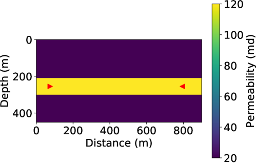
Figure 7: The scalar value of the permeability $K$ at each location. The triangular markers are point sources.

We adopt a nonlinear implicit scheme for solving the PDE system since it is unconditionally stable. We refer readers to [43] for the numerical scheme and implementation details. The nonlinear implicit step involves solving

$$\phi(S_{2}^{n+1}-S_{2}^{n})-\nabla\cdot\left({{m_{2}}(S_{2}^{n+1})K\nabla\Psi_{2}^{n}}\right)\Delta t=\left(q_{2}^{n}+q_{1}^{n}\frac{m_{2}(S^{n+1}_{2})}{m_{1}(S^{n+1}_{2})}\right)\Delta t$$ (24)

where $n$ stands for the time step $n$ and $\Delta t$ is the time step. $\Psi_{2}^{n}$ is the fluid potential and can be computed using $S_{2}^{n}$ (see [43] for details) and

$$m_{i}(s)=\frac{k_{ri}(s)}{\tilde{\mu}_{i}}$$

We apply the Newton-Raphson algorithm to solve the nonlinear equation Eq. 24. This means we need to compute $m_{i}^{\prime}(s)$. We implement an efficient custom operator for solving Eq. 24 where the linear system is solved with algebraic multi-grid methods [44, 45].

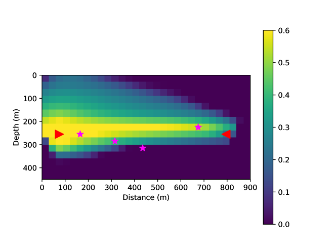
Figure 8: Source functions and locations where observations are collected. The triangular markers are point sources; to be more specific, the left source is an injection while the right source is an absorption (e.g., production wells). The four magenta markers are locations where observations are collected. The background scalar values show the saturation at the terminal time of the simulation.

We assume that we can measure the saturation $S_{1}$, denoted as $\hat{S}_{1}^{n}(\mathbf{x}_{i})$ ($n$ denotes the time step), at multiple locations $\{\mathbf{x}_{i}\}_{i\in\mathcal{I}_{\mathrm{obs}}}$ (the magenta markers in Figure 8). The saturation model Eq. 22 is unknown to us. In this setting, we cannot measure or compute $K$ and $S_{i}$ directly at all locations, and, therefore, it is impossible to build the saturation model $K_{ri}$ by direct curve fitting. Instead, we use two neural networks to approximate the saturation models

$$f_{1}(S_{1};\theta_{1})\approx k_{r1}(S_{1})\qquad f_{2}(S_{1};\theta_{2})\approx k_{r2}(S_{1})$$

where $\theta_{1}$ and $\theta_{2}$ are the weights and biases for two neural networks. The neural network is constrained to output values between $(0,1)$ by applying

$$x\mapsto\frac{\tanh(x)+1}{2}$$

to the outputs of the neural networks in the last layer.

Corresponding to Eq. 1, we have ($S_{i}^{n}$ and $P_{i}^{n}$ are solution vectors)

$$u =[S_{1}^{n}\ S_{2}^{n}\ P_{1}^{n}\ P_{2}^{n}]_{n=1,2,\ldots}$$

$$\theta =[\theta_{1}\ \theta_{2}]$$

$$L(u) =\sum_{i\in\mathcal{I}_{\mathrm{obs}}}\sum_{n}(S_{1}^{n}(\mathbf{x}_{i})-\hat{S}_{1}^{n}(\mathbf{x}_{i}))^{2}$$

and $F(u,\theta)=0$ is given by the systems of Eqns. 19, 20 and 21.

Parameter	Value
$g$	9.8
$h$	30
Time Steps	50
$\Delta t$	20
Domain	$[0,900]\times[0,450]$
$\rho_{1}$	501.9
$\rho_{2}$	1053
$\tilde{\mu}_{1}$	0.1
$\tilde{\mu}_{2}$	1
Neural Network	Fully-connected 1-20-20-20-1

Table 6: Parameters used in the simulation.

We list the parameters for carrying out the numerical simulation in Table 6. Table 7 compares the number of independent variables for PCL and the penalty method. We can see that the penalty method leads to a huge number of unknown variables, and the associated optimization problem is difficult to solve. However, the independent variables in PCL is limited to weights and biases of the neural network.

Method	PCL	Penalty Method
# Parameters	1802	24302

Table 7: Comparison of independent variables for penalty method and PCL.

Therefore, we select PCL to solve the two-phase flow inverse modeling problem. As shown in Figure 9, PCL successfully learns the saturation model in the region of physical interest. The estimation is not accurate near the boundary since there are few data points in this region. Finally, we show the true and reconstructed saturation $S_{1}$ in Figure 10 using the estimated neural network saturation model. We see the reconstructed saturation is nearly the same as true saturation.

Figure 9: Left: root mean squared error of estimated and true $k_{ri}$. Right: visualization of the neural network approximation to $k_{ri}$; this plot is generated at the 491th iteration.

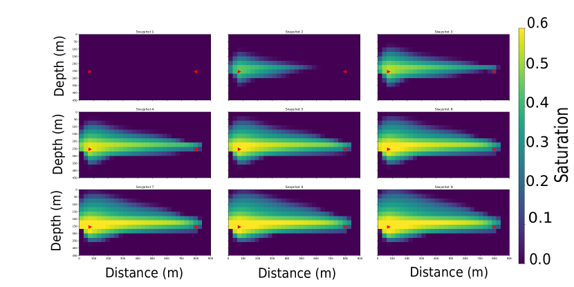
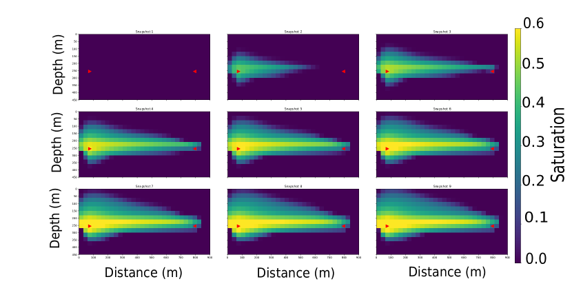
Figure 10: Saturation $S_{1}$ at Day 0, 5, 10, 15, 20, 25, 30, 35, 40 (from left to right, top to bottom). The top figure shows the true saturation computed with Eq. 22 and the bottom figure shows the saturation computed with the neural network saturation model. The distance ranges from 0 m to 900 m and the depth ranges from 0 m to 450 m.

4 Conclusion

We have compared two methods for data-driven modeling with sparse observations: the penalty method (PM) and the physics constrained learning method (PCL). The difference is that PM enforces the physical constraints by including a penalty term in the loss function, considering the solution vectors as independent variables, while PCL solves the system of PDEs directly. We proved that PM is more ill-conditioned than PCL in a model problem: the condition number of PM is the square of that of PCL asymptotically, which explains the slow convergence or divergence of PM during the optimization. The increase in the number of independent variables in PM can be very large for dynamical systems. Additionally, we proposed an approach for implementing PCL through automatic differentiation, and thus not only getting rid of the time-consuming and difficult process of deriving and implementing the gradients, but also leverages computational graph-based optimization for performance.

The proposed PCL method shows superior performance over the PM method in terms of iterations to converge. We see almost a $10^{4}$ speed-up in the Helmholtz equation example. Additionally, when we approximate the unknown function with a neural network, PM is sensitive to the choice of penalty parameters and neural network architectures, and may converge to a bad local minimum. In contrast, PCL consistently converges to the true solution for different neural network architectures and test function sets.

However, PCL suffers from some limitations compared to PM. Firstly, the memory and computation costs per iteration for PCL are greater than the penalty method; for nonlinear problems, we may need an expensive iterative method such as the Newton-Raphson algorithm for solving the nonlinear system. Secondly, for time-dependent problems, PCL must solve the equation sequentially in time. This calculation can be computationally challenging for long time horizons. However, for PM long time horizon problems are also very challenging: it has a large number of independent variables. Thirdly, from the perspective of implementation, PM only requires first-order derivatives, while PCL requires extra Jacobian matrices. As a result, PCL requires more implementation work and is generally more expensive in computation and storage per iteration.

The idea of enforcing physical constraints by solving the PDEs numerically is very crucial for learning parameters or training deep neural network surrogate models in stiff problems. To this end, physics constraint learning puts forth an effective and efficient approach that can be integrated into an automatic differentiation framework and interacts between deep learning and computational engineering. PCL allows for the potential to supplement the best of available scientific computing tools with deep learning techniques for inverse modeling.

Appendix A NURBS Domain

The same geometry can be described in many ways using NURBS. We have implemented a module in IGACS.jl with many built-in meshes and utilities to generate NURBS mesh (e.g., from boundaries described by NURBS curves). See documentation or source codes for details. We present the NURBS data structure for the meshes we have used in this paper. The meshes are subjected to refinement or affine transformation for the numerical examples in Section 3.

Table 8: Weights ($w$) and control points $(x,y)$ for the square mesh. The knot vectors are $u=(0,0,0,1,1,1)$, $v=(0,0,0,1,1,1)$ and the degrees are $p=q=2$.

$w$	$x$	$y$
1	$-1$	1
1	$-1$	0
1	$-1$	$-1$
1	0	1
1	0	0
1	0	$-1$
1	1	1
1	1	0
1	1	$-1$

Table 9: Weights ($w$) and control points $(x,y)$ for the curved pipe mesh. The knot vectors are $u=(0,0,1,1)$, $v=(0,0,0,1,1,1)$ and the degrees are $p=1$,$q=2$.

$w$	$x$	$y$
1	1	0
1	2	0
$\frac{\sqrt{2}}{2}$	1	1
$\frac{\sqrt{2}}{2}$	2	2
1	0	1
1	0	2

Figure 11: Control points (red) and boundaries of the square and curved pipe mesh.

Appendix B Isogeometric Analysis

B.1 Overview

Non-Uniform Rational B-Splines (NURBS) have been a standard tool for describing and modeling curves and surfaces in CAD programs. Isogeometric analysis uses NURBS as an analysis tool, proposed by Hughes et al [15]. In this section, we present a short description of the isogeometric collocation method (IGA-C). For details, we refer the readers to [16, 46, 47, 48, 49].

We emphasize that the isogeometric collocation method is not the only way to implement the physics constrained learning. We use IGA-C here since it has smooth basis functions and thus allows us to work with strong forms of the PDE directly. It has also been shown effective for applications in solid mechanics [15], fluid dynamics [50], etc. The physics constrained learning can also be applied to finite element analysis and other numerical discretization methods.

B.2 B-splines and NURBS

B-splines are piecewise polynomials curves, which are composed of linear combinations of B-spline basis functions. There are three components of $B$-splines:

1. Control points. Control points (denoted by $\mathbf{B}_{i}$) are points in the plane. Control points affect the shape of B-spline curves but are not necessarily on the curve.

2. Knot vector. A knot vector is a set of non-decreasing real numbers representing coordinates in the parametric space

   $$\{\xi_{1}=0,\ldots,\xi_{n+p+1}=1\}$$

   where $p$ is the degree of the B-spline and $n$ is the number of basis functions, which is equal to the number of control points. A knot vector is uniform if the knots are uniformly-spaced and non-uniform otherwise.

3. B-spline basis functions. B-spline basis functions are defined recursively by the knot vector. For $p=0$

   $$N_{i,0}(\xi)=\begin{cases}1&\mbox{ if }\xi_{i}\leq\xi<\xi_{i+1}\\ 0&\mbox{ otherwise }\end{cases}$$

   For $p>1$, we have

   $$N_{i,p}=\begin{cases}\frac{\xi-\xi_{i}}{\xi_{i+p}-\xi_{i}}N_{i,p-1}(\xi)+\frac{\xi_{i+p+1}-\xi}{\xi_{i+p+1}-\xi_{i+1}}N_{i+1,p-1}(\xi)&\mbox{ if }\xi\in[\xi_{i},\xi_{i+p+1})\\ 0&\mbox{ otherwise }\end{cases}$$

The basis functions of a 2D B-spline region $\Omega$ can be constructed by tensor product of 1D B-spline basis functions. Let $\mathbf{B}_{i,j}$, $i=1,2,\ldots,n+p+1$, $j=1,2,\ldots,m+q+1$ be the control points, where $n$, $m$ are the number of basis functions per dimension, and $p$, $q$ are degrees of the B-splines perspectively, the region can be represented as a map from the parametric space $[0,1]^{2}$ to the physical space $\Omega$

$$S(\xi,\eta)=\sum_{i=1}^{n}\sum_{j=1}^{m}N_{i,p}(\xi,\eta)M_{j,p}(\xi,\eta)\mathbf{B}_{i,j}$$

here we use $N$ and $M$ to denote the basis functions for each dimension.

Analogously to B-splines, the basis functions for NURBS in a 2D domain are defined as

$$R_{i,j}^{p,q}(\xi,\eta)=\frac{N_{i,p}(\xi)M_{j,q}(\eta)w_{i,j}}{\sum_{i=1}^{n}\sum_{j=1}^{m}N_{i,p}(\xi)M_{j,q}(\eta)w_{i,j}}$$

where $w_{i,j}$ are called weights of the NURBS surface. Hence the NURBS mapping is

$$R(\xi,\eta)=\sum_{i=1}^{n}\sum_{j=1}^{m}R_{i,j}^{p,q}(\xi,\eta)\mathbf{B}_{i,j}$$

B.3 Isogeometric Collocation Method

In the isogeometric collocation method, the solution to the PDE is represented as a linear combination of NURBS basis functions

$$u_{h}(\mathbf{x})=\sum_{i=1}^{n}\sum_{j=1}^{m}c_{i,j}R_{i,j}^{p,q}(\xi,\eta)\quad\mathbf{x}=\sum_{i=1}^{n}\sum_{j=1}^{m}R_{i,j}^{p,q}(\xi,\eta)\mathbf{B}_{i,j}$$

here $c_{i,j}\in\mathbb{R}$ are the coefficients of the basis functions. The smoothness of $u_{h}(\mathbf{x})$ depends on the continuity of the basis function $R_{i,j}$, which, in turn, depends on the continuity of $\{N_{i,p}\}$, $\{M_{j,p}\}$. $N_{i,p}$ is smooth between knots in the knot vector and $C^{p-k}$ where $k$ is the multiplicity of $u_{l}$ at the knot $u_{l}$; the same is true for $M_{j,p}$. Therefore, we can make $u_{h}(x)$ arbitrarily smooth by selecting appropriate knot vectors and degrees.

Since $u_{h}(x)$ can be made continuously differentiable up to any order, we can work directly with the strong form of PDEs. Consider a linear boundary-value problem ($\mathcal{P}$ and $\mathcal{B}$ are linear differential operators)

$$\mathcal{P}u =f \mbox{ in }\Omega$$ (25)

$$\mathcal{B}u =g \mbox{ on }\Omega$$

The isogeometric collocation method solves the problem by finding the coefficients $c_{i,j}$ that satisfies

$$\sum_{i=1}^{n}\sum_{j=1}^{m}c_{i,j}\mathcal{P}\Big{(}R_{i,j}^{p,q}\Big{)}(\xi_{l},\eta_{l}) =f(R(\xi_{l},\eta_{l})), l\in\mathcal{I}_{P}$$ (26)

$$\sum_{i=1}^{n}\sum_{j=1}^{m}c_{i,j}\mathcal{B}\Big{(}R_{i,j}^{p,q}\Big{)}(\xi_{l},\eta_{l}) =g(R(\xi_{l},\eta_{l})), l\in\mathcal{I}_{B}$$

here $\{(\xi_{l},\eta_{l})\}$ are tensor products of the Greville abscissae, and $\mathcal{I}_{P}$, $\mathcal{I}_{B}$ refer to the indices corresponding to inner and boundary points. $\mathcal{P}\Big{(}R_{i,j}^{p,q}\Big{)}$ and $\mathcal{B}\Big{(}R_{i,j}^{p,q}\Big{)}$ can be precomputed with efficient De Boor’s algorithm. Eq. 26 leads to a sparse linear system

$$\mathbf{A}\mathbf{c}=\mathbf{f}\quad\mathbf{c}=\begin{bmatrix}c_{11}\\ c_{12}\\ \vdots\\ c_{1n}\\ c_{21}\\ \vdots\\ c_{mn}\end{bmatrix}\quad\mathbf{f}=\begin{bmatrix}f(R(\xi_{1},\eta_{1}))\\ f(R(\xi_{1},\eta_{2}))\\ \vdots\\ f(R(\xi_{1},\eta_{n}))\\ f(R(\xi_{2},\eta_{1}))\\ \vdots\\ f(R(\xi_{m},\eta_{n}))\end{bmatrix}$$

where $\mathbf{A}$ is a sparse matrix. When Eq. 25 is nonlinear, the Newton–Raphson algorithm is used to find the coefficients.

Appendix C Automatic Differentiation

We give a short introduction to automatic differentiation. We do not attempt to cover the details in automatic differentiation since there is extensive literature (see [31] for a comprehensive review) on this topic; instead, we only discuss the relevant techniques associated with physics constrained learning.

We describe the reverse mode automatic differentiation. Assume we are given inputs

$$\{x_{1},x_{2},\ldots,x_{n}\}$$

and the algorithm produces a single output $x_{N}$, $N>n$. The gradients

$$\frac{\partial x_{N}(x_{1},x_{2},\ldots,x_{n})}{\partial x_{i}}$$

$i=1$, $2$, $\ldots$, $n$ are queried.

The idea is that this algorithm can be decomposed into a sequence of functions $f_{i}$ ($i=n+1,n+2,\ldots,N$) that can be easily differentiated analytically, such as addition, multiplication, or basic functions like exponential, logarithm and trigonometric functions. Mathematically, we can formulate it as

$$x_{n+1} =f_{n+1}(\mathbf{x}_{\pi({n+1})})$$

$$x_{n+2} =f_{n+2}(\mathbf{x}_{\pi({n+2})})$$

$$\ldots$$

$$x_{N} =f_{N}(\mathbf{x}_{\pi({N})})$$

where $\mathbf{x}=\{x_{i}\}_{i=1}^{N}$ and $\pi(i)$ are the parents of $x_{i}$, s.t., $\pi(i)\in\{1,2,\ldots,i-1\}$.

The idea to compute $\partial x_{N}/\partial x_{i}$ is to start from $i=N$, and establish recurrences to calculate derivatives with respect to $x_{i}$ in terms of derivatives with respect to $x_{j}$, $j>i$. To define these recurrences rigorously, we need to define different functions that differ by the choice of independent variables.

The starting point is to define $x_{i}$ considering all previous $x_{j}$, $j<i$, as independent variables. Then:

$$x_{i}(x_{1},x_{2},\ldots,x_{i-1})=f_{i}(\mathbf{x}_{\pi(i)})$$

Next, we observe that $x_{i-1}$ is a function of previous $x_{j}$, $j<i-1$, and so on; so that we can recursively define $x_{i}$ in terms of fewer independent variables, say in terms of $x_{1}$, …, $x_{k}$, with $k<i-1$. This is done recursively using the following definition:

$$x_{i}(x_{1},x_{2},\ldots,x_{j})=x_{i}(x_{1},x_{2},\ldots,x_{j},f_{j+1}(\mathbf{x}_{\pi(j+1)})),\quad n<j+1<i$$

Observe that the function of the left-hand side has $j$ arguments, while the function on the right has $j+1$ arguments. This equation is used to “reduce” the number of arguments in $x_{i}$.

With these definitions, we can define recurrences for our partial derivatives which form the basis of the back-propagation algorithm. The partial derivatives for

$$x_{N}(x_{1},x_{2},\ldots,x_{N-1})$$

are readily available since we can differentiate

$$f_{N}(\mathbf{x}_{\pi(N)})$$

directly. The problem is therefore to calculate partial derivatives for functions of the type $x_{N}(x_{1},x_{2},\ldots,x_{i})$ with $i<N-1$. This is done using the following recurrence:

$$\frac{\partial x_{N}(x_{1},x_{2},\ldots,x_{i})}{\partial x_{i}}=\sum_{j\,:\,i\in\pi(j)}\frac{\partial x_{N}(x_{1},x_{2},\ldots,x_{j})}{\partial x_{j}}\frac{\partial x_{j}(x_{1},x_{2},\ldots,x_{j-1})}{\partial x_{i}}$$

with $n<i<N-1$. Since $i\in\pi(j)$, we have $i<j$. So we are defining derivatives with respect to $x_{i}$ in terms of derivatives with respect to $x_{j}$ with $j>i$. The last term

$$\frac{\partial x_{j}(x_{1},x_{2},\ldots,x_{j-1})}{\partial x_{k}}$$

is readily available since:

$$x_{j}(x_{1},x_{2},\ldots,x_{j-1})=f_{j}(\mathbf{x}_{\pi(j)})$$

The computational cost of this recurrence is proportional to the number of edges in the computational graph (excluding the nodes $1$ through $n$), assuming that the cost of differentiating $f_{k}$ is $O(1)$. The last step is defining

$$\frac{\partial x_{N}(x_{1},x_{2},\ldots,x_{n})}{\partial x_{i}}=\sum_{j\,:\,i\in\pi(j)}\frac{\partial x_{N}(x_{1},x_{2},\ldots,x_{j})}{\partial x_{j}}\frac{\partial x_{j}(x_{1},x_{2},\ldots,x_{j-1})}{\partial x_{i}}$$

with $1\leq i\leq n$. Since $n<j$, the first term

$$\frac{\partial x_{N}(x_{1},x_{2},\ldots,x_{j})}{\partial x_{j}}$$

has already been computed in earlier steps of the algorithm. The computational cost is equal to the number of edges connected to one of the nodes in $\{1,\dots,n\}$.

We can see that the complexity of the back-propagation is bounded by that of the forward step, up to a constant factor. Reverse mode differentiation is very useful in the penalty method, where the loss function is a scalar, and no other constraints are present.

Appendix D Automatic Jacobian Calculation

When the constraint $F_{h}(\theta,u_{h})=0$ is nonlinear, we need extra effort to compute the Jacobian

$$\frac{{\partial{F_{h}}}}{{\partial{u_{h}}}}(\theta,u_{h})\Bigg{|}_{u_{h}={G_{h}}(\theta)}$$

for both the forward modeling (e.g., the Jacobian is used in Newton-Raphson iteration for solving nonlinear systems) and computing the gradient Eq. 6. This should not be confused with reverse mode automatic differentiation: the technique described in this section is only used for computing sparse Jacobians; when computing the gradient Eq. 6, on top of the Jacobians, the reverse mode automatic differentiation is applied to extract gradients (F). For efficiency, it is desired that we can exploit the sparsity of the Jacobian term.

In this section, we describe a method for automatically computing the sparse Jacobian matrix. This method is not restricted to the numerical methods we use in our numerical examples (finite difference and isogeometric analysis) and can be extended to most commonly used numerical schemes such as finite element analysis and finite volume methods.

The technique used here is similar to forward mode automatic differentiation. The difference is that we pass the sparse Jacobian matrices in the computational graph instead of gradient vectors. The locality of differential operators is the key to preserving the sparsity of those Jacobian matrices. The major three steps of our method for computing Jacobians automatically are

1. Building the computational graph;

2. For each operator in the computational graph, implementing the differentiation rule with respect to its input;

3. Pushing the sparse Jacobians through the computational graph with chain rules in the same order as the operators of the forward modeling.

We consider a specific example to illustrate our algorithm. Assume that the numerical solution is represented by a linear combination of basis functions such as isogeometric analysis, $u_{\mathbf{c}}$, where $\mathbf{c}$ is the coefficients. Let the physical constraint and its discretization be (we omit parameters $\theta$ here since it is irrelevant)

$$F(u)=\nabla\cdot((1+u^{2})\nabla u)\qquad F_{h}(u_{\mathbf{c}})=\nabla\cdot((1+u_{\mathbf{c}}^{2})\nabla u_{\mathbf{c}})$$

We want to compute the Jacobian matrix

$$J(\mathbf{c})=\frac{\partial F_{h}(u_{\mathbf{c}})}{\partial\mathbf{c}}$$ (27)

Now we decompose the operator into several individual operators in the computational graph (Figure 12)

$$F_{0}(\mathbf{c})= \;u_{\mathbf{c}}=M\mathbf{c}$$

$$F_{1}(\mathbf{c})= \;\nabla F_{0}(\mathbf{c})=[M_{x}F_{0}(\mathbf{c})\ M_{y}F_{0}(\mathbf{c})]$$

$$F_{2}(\mathbf{c})= \;F_{0}(\mathbf{c})^{2}$$

$$F_{3}(\mathbf{c})= \;1+F_{2}(\mathbf{c})$$

$$F_{4}(\mathbf{c})= \;F_{3}(\mathbf{c})F_{1}(\mathbf{c})$$

$$F_{5}(\mathbf{c})= \;\nabla\cdot F_{4}(\mathbf{c})$$

here $M$ is the coefficient matrix for numerical representation of the solution $u$, $M_{x}$ and $M_{y}$ are coefficient matrices for the numerical representation of $\frac{\partial}{\partial x}$ and $\frac{\partial}{\partial y}$ associated with the selected basis functions (they can be obtained analytically by differentiating the basis functions) and all the operations denote component-wise operations, for example,

$$[F_{0}(\mathbf{c})^{2}]_{i}= \;F_{0}(\mathbf{c})_{i}^{2}$$

$$[\nabla F_{0}(\mathbf{c})]_{ik}= \;\nabla[\big{(}F_{0}(\mathbf{c})_{i}\big{)}]_{k}$$

$$[F_{3}(\mathbf{c})F_{1}(\mathbf{c})]_{ik}= \;F_{3}(\mathbf{c})_{i}F_{1}(\mathbf{c})_{ik}\quad k=1,2$$

$$[\nabla\cdot F_{4}(\mathbf{c})]_{i}= \;\nabla\cdot[F_{4}(\mathbf{c})_{i1}\ F_{4}(\mathbf{c})_{i2}]$$

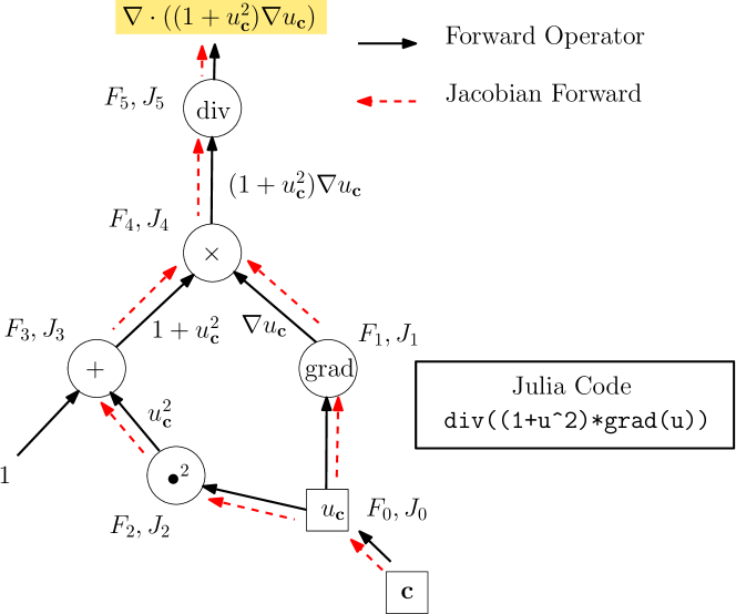
Figure 12: Jacobian forward propagation in the computational graph. The Jacobian computation is automatic: the users only need to specify the forward operations.

The corresponding differentiation rule for each operator is

$${J_{0}(\mathbf{c})}= \;\frac{\partial}{\partial\mathbf{c}}F_{0}(\mathbf{c})=M$$

$${J_{1}(\mathbf{c})}= \;\frac{\partial}{\partial\mathbf{c}}F_{1}(\mathbf{c})=[M_{x}{J_{0}(\mathbf{c})}\ M_{y}{J_{0}(\mathbf{c})}]$$

$${J_{2}(\mathbf{c})}= \;\frac{\partial}{\partial\mathbf{c}}F_{2}(\mathbf{c})=2\mathrm{diag}(F_{0}(\mathbf{c})){J_{0}(\mathbf{c})}$$

$${J_{3}(\mathbf{c})}= \;\frac{\partial}{\partial\mathbf{c}}F_{3}(\mathbf{c})={J_{2}(\mathbf{c})}$$

$${J_{4}(\mathbf{c})}= \;\frac{\partial}{\partial\mathbf{c}}F_{4}(\mathbf{c})=2\mathrm{diag}(F_{3}(\mathbf{c})){J_{1}(\mathbf{c})}$$

$$+[\mathrm{diag}(M_{x}F_{0}(\mathbf{c})){J_{3}(\mathbf{c})}\ \mathrm{diag}(M_{y}F_{0}(\mathbf{c})){J_{3}(\mathbf{c})}]$$

$${J_{5}(\mathbf{c})}= \;\frac{\partial}{\partial\mathbf{c}}F_{5}(\mathbf{c})={J_{4}(\mathbf{c})}\begin{bmatrix}M_{x}\\ M_{y}\end{bmatrix}$$

Here $\mathrm{diag}(\mathbf{v})$ denotes the diagonal matrix whose diagonal entries are $\mathbf{v}$. By chaining together all the differentiation rules, $J_{5}(\mathbf{c})=J(\mathbf{c})$ is the desired Jacobian. We can see the dependency of $J_{k}(\mathbf{c})$, $k=1$, …, $5$ is the same as the forward modeling, which also explains why the dashed red arrows (Jacobian Forward) in Figure 12 parallel the forward computation. The order of the computation is different from reverse mode automatic differentiation in Eq. 6. Reverse mode automatic differentiation is most efficient when the final output is a scalar value. $F(u,\theta)$ is a multiple input multiple output operator and therefore computing $\frac{\partial F(u,\theta)}{\partial u}$ using reverse mode automatic differentiation is inefficient. Nevertheless, $F(u,\theta)$ is composed of differential operators and our representation of the solution $u$ consists of local basis functions. This locality enables us to obtain an efficient automatic Jacobian calculation algorithm that preserves the sparsity.

Appendix E Automatic Jacobian Calculation Implementation in
IGACS.jl

It is useful to have an understanding of how we implement automatic Jacobian calculation in IGACS.jl. The implementation can also be extended to other basis functions or weak formulations such as finite difference method, finite element method, and finite volume method. It is also possible to extend to global basis functions by back-propagating special structured matrices instead of sparse Jacobian matrices.

The automatic Jacobian calculation implementation is based on
ADCME.jl [51], which leverages TensorFlow [20, 21] for graph optimization and numerical acceleration (e.g., XLA, CUDA). The computational graph parsing and bookkeeping are done in Julia [52], which does not affect runtime performance. ADCME.jl also implements a sparse linear algebra custom operator library to augment the built-in tf.sparse in TensorFlow. In sum, we have made our best effort to attain high performance of IGACS.jl by leveraging TensorFlow and customizing performance critical computations.

One important concern for designing IGACS.jl is the accessibility to users. We hide the details of gradients back-propagation or Jacobian forward-propagation by abstraction via the structure Coefficient, which holds the data of the NURBS representation and tracing information in the computational graph. For example, to compute $J(c)=\nabla\cdot((1+c^{2})\nabla c)$, users can simply write

$$\texttt{J}=\texttt{div}((1+\texttt{c}^{2})*\texttt{grad}(\texttt{c}))$$

This will build the computational graph automatically. For computing Jacobian, users only need to write

$$\texttt{deriv}(\texttt{J},\texttt{c})$$

This will parse the dependency of the computational graph and return a sparse matrix (SparseTensor struct in ADCME) at the Greville abscissae (other collocation points can be specified by passing an augment).

As an example, let the loss function be

$$L(\mu)=\int_{\Omega}\nabla\cdot((1+\mu c^{2})\nabla c)d\mathbf{x},\quad\mu\in\mathbb{R}$$

To compute the gradient $\frac{\partial L}{\partial\mu}$, we need to write

$$\texttt{J}=\texttt{div}((1+\mu*\texttt{c}^{2})*\texttt{grad}(\texttt{c}))$$

$$\texttt{g}=\texttt{gradients}(\texttt{J},\mu)$$

Appendix F Computing the Gradient with AD

Having introduced the technical tools AD and automatic Jacobian calculation, we can describe the numerical procedure for computing Eq. 6

$$\frac{{\partial{{\tilde{L}}_{h}}(\theta)}}{{\partial\theta}}=-\frac{{\partial{L_{h}}({u_{h}})}}{{\partial{u_{h}}}}{\left({\frac{{\partial{F_{h}}}}{{\partial{u_{h}}}}\Bigg{|}_{u_{h}={G_{h}}(\theta)}}\right)^{-1}}\frac{{\partial{F_{h}}}}{{\partial\theta}}(\theta,{G_{h}}(\theta))$$ (28)

For efficiency, we do not compute

$$\frac{{\partial{L_{h}}({u_{h}})}}{{\partial{u_{h}}}},\qquad{\left({\frac{{\partial{F_{h}}}}{{\partial{u_{h}}}}\Bigg{|}_{u_{h}={G_{h}}(\theta)}}\right)^{-1}},\qquad\frac{{\partial{F_{h}}}}{{\partial\theta}}(\theta,{G_{h}}(\theta))$$

separately. Instead, we take advantage of reverse mode automatic differentiation and sparse linear algebra.

First, we compute $\frac{{\partial{L_{h}}({u_{h}})}}{{\partial{u_{h}}}}$. Since $L_{h}:\mathbb{R}^{n}\rightarrow\mathbb{R}$, we can apply the reverse mode automatic differentiation to compute the gradients.

Next, computing

$$x=\frac{{\partial{L_{h}}({u_{h}})}}{{\partial{u_{h}}}}{\Big{(}{\frac{{\partial{F_{h}}}}{{\partial{u_{h}}}}\Bigg{|}_{u_{h}={G_{h}}(\theta)}}\Big{)}^{-1}}$$

is equivalent to solving a linear system

$$x\;\frac{{\partial{F_{h}}}}{{\partial{u_{h}}}}\Bigg{|}_{u_{h}={G_{h}}(\theta)}=\frac{{\partial{L_{h}}({u_{h}})}}{{\partial{u_{h}}}}$$ (29)

The term

$${\frac{{\partial{F_{h}}}}{{\partial{u_{h}}}}\Bigg{|}_{u_{h}={G_{h}}(\theta)}}$$

is computed with automatic Jacobian calculation and is sparse. Therefore, we can solve the linear system Eq. 29 with a sparse linear solver.

Consequently, we have according to Eq. 28 (in principle, $x$ depends on $\theta$; but in the equation below, we treat $x$ as independent of $\theta$)

$$\frac{{\partial{{\tilde{L}}_{h}}(\theta)}}{{\partial\theta}}=-x\frac{{\partial{F_{h}}}}{{\partial\theta}}(\theta,u_{h})\Big{|}_{u_{h}=G_{h}(\theta)}=\frac{\partial\Big{(}-xF_{h}\big{(}\theta,u_{h}\big{)}\Big{)}}{\partial\theta}\Bigg{|}_{u_{h}=G_{h}(\theta)}$$ (30)

Note that

$$\theta\mapsto-x^{T}F_{h}(\theta,u_{h})$$

is a mapping from $\mathbb{R}^{d}$ to $\mathbb{R}$, we can again apply the reverse mode automatic differentiation to compute the gradients Eq. 6.

The following code snippet shows a possible implementation of the discussion above

    l  = L(u)
    r  = F(theta, u)
    g  = gradients(l, u)
    x  = dF’\g
    x  = independent(x)
    dL = -gradients(sum(r*x), theta)

here dF is the sparse Jacobian computed with automatic Jacobian calculation. Here independent is the programmatic way of treating $x$ as independent of $\theta$.

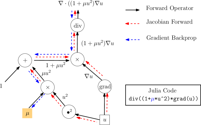
Figure 13: Forward-Backward pattern in constraint enforcement method. In each iteration, a forward simulation is performed first (black and red arrows). A gradient back-propagation (blue arrows) follows and updates the unknown parameter $\mu$.

In the inverse modeling optimization process, for each iteration, we need a forward simulation where we populate each edge with intermediate data and Jacobian matrices. Then a gradient back-propagation follows and updates the unknown parameters (Figure 13). This forward-backward pattern also exists in the penalty method, but no Jacobian information is required.

References

- [1] Victor Isakov. Inverse problems for partial differential equations, volume 127. Springer, 2006.
- [2] Jean Virieux, Amir Asnaashari, Romain Brossier, Ludovic Métivier, Alessandra Ribodetti, and Wei Zhou. An introduction to full waveform inversion. In Encyclopedia of exploration geophysics, pages R1–1. Society of Exploration Geophysicists, 2017.
- [3] Michel Grédiac and François Hild. Full-field measurements and identification in solid mechanics. John Wiley & Sons, 2012.
- [4] Volkan Akçelik, George Biros, Omar Ghattas, Judith Hill, David Keyes, and Bart van Bloemen Waanders. Parallel algorithms for PDE-constrained optimization. In Parallel processing for scientific computing, pages 291–322. SIAM, 2006.
- [5] Daniel Z. Huang, Kailai Xu, Charbel Farhat, and Eric Darve. Learning constitutive relations from indirect observations using deep neural networks, 2019.
- [6] Alexandre M Tartakovsky, Carlos Ortiz Marrero, Paris Perdikaris, Guzel D Tartakovsky, and David Barajas-Solano. Learning parameters and constitutive relationships with physics informed deep neural networks. arXiv preprint arXiv:1808.03398, 2018.
- [7] Xuhui Meng and George Em Karniadakis. A composite neural network that learns from multi-fidelity data: Application to function approximation and inverse PDE problems. arXiv preprint arXiv:1903.00104, 2019.
- [8] R-E Plessix. A review of the adjoint-state method for computing the gradient of a functional with geophysical applications. Geophysical Journal International, 167(2):495–503, 2006.
- [9] Andrew M Bradley. PDE-constrained optimization and the adjoint method. 2010.
- [10] Shingyu Leung, Jianliang Qian, et al. An adjoint state method for three-dimensional transmission traveltime tomography using first-arrivals. Communications in Mathematical Sciences, 4(1):249–266, 2006.
- [11] Grégoire Allaire. A review of adjoint methods for sensitivity analysis, uncertainty quantification and optimization in numerical codes. 2015.
- [12] Thomas Lauß, Stefan Oberpeilsteiner, Wolfgang Steiner, and Karin Nachbagauer. The discrete adjoint method for parameter identification in multibody system dynamics. Multibody system dynamics, 42(4):397–410, 2018.
- [13] James William Thomas. Numerical partial differential equations: finite difference methods, volume 22. Springer Science & Business Media, 2013.
- [14] John Noye. Finite difference techniques for partial differential equations. In North-Holland mathematics studies, volume 83, pages 95–354. Elsevier, 1984.
- [15] Thomas JR Hughes, John A Cottrell, and Yuri Bazilevs. Isogeometric analysis: CAD, finite elements, NURBS, exact geometry and mesh refinement. Computer methods in applied mechanics and engineering, 194(39-41):4135–4195, 2005.
- [16] F Auricchio, L Beirao Da Veiga, TJR Hughes, A_ Reali, and G Sangalli. Isogeometric collocation methods. Mathematical Models and Methods in Applied Sciences, 20(11):2075–2107, 2010.
- [17] Tristan van Leeuwen and Felix J Herrmann. A penalty method for PDE-constrained optimization in inverse problems. Inverse Problems, 32(1):015007, 2015.
- [18] Roland Herzog and Karl Kunisch. Algorithms for PDE-constrained optimization. GAMM-Mitteilungen, 33(2):163–176, 2010.
- [19] Adam Paszke, Sam Gross, Soumith Chintala, Gregory Chanan, Edward Yang, Zachary DeVito, Zeming Lin, Alban Desmaison, Luca Antiga, and Adam Lerer. Automatic differentiation in PyTorch. 2017.
- [20] Martín Abadi, Paul Barham, Jianmin Chen, Zhifeng Chen, Andy Davis, Jeffrey Dean, Matthieu Devin, Sanjay Ghemawat, Geoffrey Irving, Michael Isard, et al. Tensorflow: A system for large-scale machine learning. In 12th USENIX Symposium on Operating Systems Design and Implementation (OSDI 16), pages 265–283, 2016.
- [21] Martín Abadi, Ashish Agarwal, Paul Barham, Eugene Brevdo, Zhifeng Chen, Craig Citro, Greg S Corrado, Andy Davis, Jeffrey Dean, Matthieu Devin, et al. Tensorflow: Large-scale machine learning on heterogeneous distributed systems. arXiv preprint arXiv:1603.04467, 2016.
- [22] Bart van Merriënboer, Olivier Breuleux, Arnaud Bergeron, and Pascal Lamblin. Automatic differentiation in ML: Where we are and where we should be going. In Advances in neural information processing systems, pages 8757–8767, 2018.
- [23] Bradley M Bell and James V Burke. Algorithmic differentiation of implicit functions and optimal values. In Advances in Automatic Differentiation, pages 67–77. Springer, 2008.
- [24] Maziar Raissi, Paris Perdikaris, and George E Karniadakis. Physics-informed neural networks: A deep learning framework for solving forward and inverse problems involving nonlinear partial differential equations. Journal of Computational Physics, 378:686–707, 2019.
- [25] Maziar Raissi, Zhicheng Wang, Michael S Triantafyllou, and George Em Karniadakis. Deep learning of vortex-induced vibrations. Journal of Fluid Mechanics, 861:119–137, 2019.
- [26] Liu Yang, Dongkun Zhang, and George Em Karniadakis. Physics-informed generative adversarial networks for stochastic differential equations. arXiv preprint arXiv:1811.02033, 2018.
- [27] Rolf Roth and Stefan Ulbrich. A discrete adjoint approach for the optimization of unsteady turbulent flows. Flow, turbulence and combustion, 90(4):763–783, 2013.
- [28] Tyrone Rees, H Sue Dollar, and Andrew J Wathen. Optimal solvers for PDE-constrained optimization. SIAM Journal on Scientific Computing, 32(1):271–298, 2010.
- [29] Simon W Funke and Patrick E Farrell. A framework for automated PDE-constrained optimisation. arXiv preprint arXiv:1302.3894, 2013.
- [30] Aurel Galántai. The theory of Newton’s method. Journal of Computational and Applied Mathematics, 124(1-2):25–44, 2000.
- [31] Atilim Gunes Baydin, Barak A Pearlmutter, Alexey Andreyevich Radul, and Jeffrey Mark Siskind. Automatic differentiation in machine learning: a survey. Journal of machine learning research, 18(153), 2018.
- [32] David G Luenberger, Yinyu Ye, et al. Linear and nonlinear programming, volume 2. Springer, 1984.
- [33] Andreas Griewank and Andrea Walther. Evaluating derivatives: principles and techniques of algorithmic differentiation, volume 105. Siam, 2008.
- [34] Charles C Margossian. A review of automatic differentiation and its efficient implementation. Wiley Interdisciplinary Reviews: Data Mining and Knowledge Discovery, page e1305, 2018.
- [35] Nevena Jakovčević Stor, Ivan Slapničar, and Jesse Barlow. Accurate eigenvalue decomposition of arrowhead matrices, rank-one modifications of diagonal matrices and applications. In International Workshop on Accurate Solution of Eigenvalue Problems X, 2014.
- [36] Joseph-Frédéric Bonnans, Jean Charles Gilbert, Claude Lemaréchal, and Claudia A Sagastizábal. Numerical optimization: theoretical and practical aspects. Springer Science & Business Media, 2006.
- [37] Yunmei Chen and Vladimir Rokhlin. On the inverse scattering problem for the Helmholtz equation in one dimension. Inverse Problems, 8(3):365, 1992.
- [38] Gang Bao and Peijun Li. Inverse medium scattering for the Helmholtz equation at fixed frequency. Inverse Problems, 21(5):1621, 2005.
- [39] M Tadi, AK Nandakumaran, and SS Sritharan. An inverse problem for Helmholtz equation. Inverse Problems in Science and Engineering, 19(6):839–854, 2011.
- [40] Cl Kleinstreuer. Two-phase flow: theory and applications. Routledge, 2017.
- [41] Royal Harvard Brooks and Arthur T Corey. Properties of porous media affecting fluid flow. Journal of the irrigation and drainage division, 92(2):61–90, 1966.
- [42] Frode Lomeland, Einar Ebeltoft, and Wibeke Hammervold Thomas. A new versatile relative permeability correlation. In International Symposium of the Society of Core Analysts, Toronto, Canada, volume 112, 2005.
- [43] Dongzhuo Li, Kailai Xu, Jerry M Harris, and Eric Darve. Time-lapse full waveform inversion for subsurface flow problems with intelligent automatic differentiation. arXiv preprint arXiv:1912.07552, 2019.
- [44] Denis Demidov. Amgcl: an efficient, flexible, and extensible algebraic multigrid implementation. Lobachevskii Journal of Mathematics, 40(5):535–546, 2019.
- [45] Xiaozhe Hu, Wei Liu, Guan Qin, Jinchao Xu, Zhensong Zhang, et al. Development of a fast auxiliary subspace pre-conditioner for numerical reservoir simulators. In SPE Reservoir Characterisation and Simulation Conference and Exhibition. Society of Petroleum Engineers, 2011.
- [46] J Austin Cottrell, Thomas JR Hughes, and Yuri Bazilevs. Isogeometric analysis: toward integration of CAD and FEA. John Wiley & Sons, 2009.
- [47] Thomas JR Hughes, Alessandro Reali, and Giancarlo Sangalli. Efficient quadrature for NURBS-based isogeometric analysis. Computer methods in applied mechanics and engineering, 199(5-8):301–313, 2010.
- [48] Yuri Bazilevs, L Beirao da Veiga, J Austin Cottrell, Thomas JR Hughes, and Giancarlo Sangalli. Isogeometric analysis: approximation, stability and error estimates for h-refined meshes. Mathematical Models and Methods in Applied Sciences, 16(07):1031–1090, 2006.
- [49] Vinh Phu Nguyen, Cosmin Anitescu, Stéphane PA Bordas, and Timon Rabczuk. Isogeometric analysis: an overview and computer implementation aspects. Mathematics and Computers in Simulation, 117:89–116, 2015.
- [50] Peter Nørtoft Nielsen, Allan Roulund Gersborg, Jens Gravesen, and Niels Leergaard Pedersen. Discretizations in isogeometric analysis of navier–stokes flow. Computer methods in applied mechanics and engineering, 200(45-46):3242–3253, 2011.
- [51] Kailai Xu and Eric Darve. Physics based machine learning for inverse problems. https://kailaix.github.io/ADCME.jl/dev/assets/Slide/ADCME.pdf.
- [52] Jeff Bezanson, Stefan Karpinski, Viral B. Shah, and Alan Edelman. Julia: A fast dynamic language for technical computing. CoRR, abs/1209.5145, 2012.