Topological Edge and Interface states at Bulk disorder-to-order
Quantum Critical Points

Abstract

We study the interplay between two nontrivial boundary effects: (1) the two dimensional ($2d$) edge states of three dimensional ($3d$) strongly interacting bosonic symmetry protected topological states, and (2) the boundary fluctuations of $3d$ bulk disorder-to-order phase transitions. We then generalize our study to $2d$ gapless states localized at an interface embedded in a $3d$ bulk, when the bulk undergoes a quantum phase transition. Our study is based on generic long wavelength descriptions of these systems and controlled analytic calculations. Our results are summarized as follows: ($i.$) The edge state of a prototype bosonic symmetry protected states can be driven to a new fixed point by coupling to the boundary fluctuations of a bulk quantum phase transition; ($ii.$) the states localized at a $2d$ interface of a $3d$ ${\rm SU}(N)$ quantum antiferromagnet may be driven to a new fixed point by coupling to the bulk quantum critical modes. Properties of the new fixed points identified are also studied.

I Introduction

The most prominent feature of topological insulators (TI) Kane and Mele (2005a, b); Fu et al. (2008); Moore and Balents (2007); Schnyder et al. (2009); Ryu et al. (2010); Kitaev (2009) and more generally symmetry protected topological (SPT) states Chen et al. (2013, 2012) is the contrast between the boundary and the bulk of the system. In particular the $2d$ edge of $3d$ SPT states hosts the most diverse zoo of exotic phenomena that keep attracting attentions and efforts from theoretical physics. It has been shown that many exotic phenomena such as anomalous topological order Fidkowski et al. (2013); Chen et al. (2014); Bonderson et al. (2013); Wang et al. (2013); Metlitski et al. (2013); Wang and Senthil (2013); Cheng et al. (2016), deconfined quantum critical points Vishwanath and Senthil (2013), self-dual field theories Xu and You (2015); Mross et al. (2016); Hsin and Seiberg (2016); Wang et al. (2017) can all occur on the $2d$ edge of $3d$ SPT stats. Sometimes the symmetry of the system is secretly realized as a self-dual transformation of the field theories at the boundary Seiberg et al. (2016); Senthil et al. (2019). All these suggest that the $2d$ boundary of a $3d$ system is an ideal platform of studying physics beyond the standard frameworks of condensed matter theory.

On the other hand, even the boundary of an ordinary Landau-Ginzburg type of quantum phase transition can have nontrivial behaviors. It was studied and understood in the past that the boundary of a bulk conformal field theory (CFT) follows a very different critical behavior from the bulk Cardy (1996, 1984); Dietrich and Diehl (1983); Diehl and Dietrich (1981); Reeve and Guttmann (1981); Diehl (1997), due to the strong boundary condition imposed on the CFT. The boundary fluctuations (or the boundary CFT) of the Landau-Ginzburg phase transitions were studied through the standard $\epsilon-$expansion, and it was shown that the critical exponents are very different from the bulk. Hence if experiments are performed at the boundary of the system, one should refer to the predictions of the boundary instead of the bulk CFT. These two different boundary effects were studied separately in the past. In this work we will study the interplay of these two distinct boundary effects. Our goal is to seek for new physics, ideally new fixed points under renormalization group (RG) flow due to the coupling of the two boundary effects.

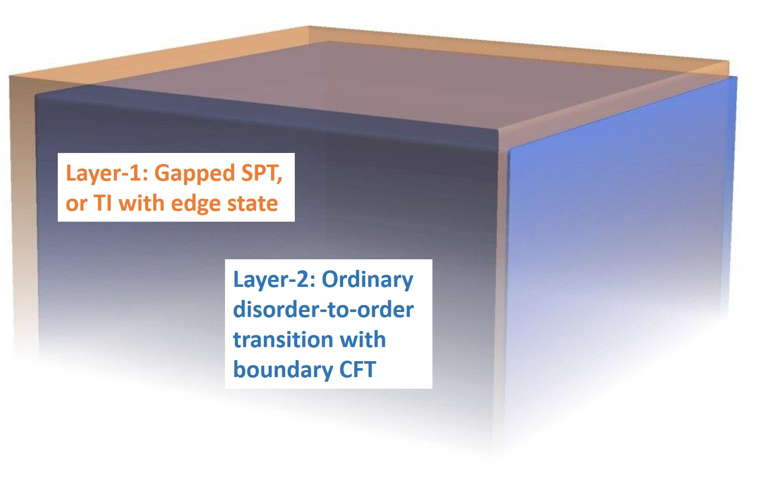
Figure 1: We view the system under study as a two layer system. Layer-1 is a SPT or TI with nontrivial edge states; layer-2 is an ordinary disorder-to-order phase transition whose order parameter at the boundary follows the scaling of boundary CFT. The boundary of the entire system may flow to new fixed points due to the coupling between the two layers.

For our purpose we give the system under study a virtual two-layer structure Fig. 1: layer-1 is a SPT state with nontrivial edge states, and it is not tuned to a bulk phase transition; layer-2 is a topological trivial system which undergoes an ordinary Landau-Ginzburg disorder-to-order phase transition. Then as a starting point we assume a weak coupling between the boundary of the two layers, and study the RG flow of the coupling. Besides the edge state localized at the boundary of a SPT state, we will also consider symmetry protected gapless states localized at a $2d$ interface embedded in a $3d$ bulk. We will demonstrate that in several cases, including the edge state of a prototype bosonic SPT state, the $2d$ boundary or interface will flow to a new fixed point due to the bulk quantum phase transition.

Previous works have explored related ideas with different approaches. Exactly soluble $1d$ and $2d$ Hamiltonians have been constructed for gapless systems with protected edge states Scaffidi et al. (2017); fate of edge states was also studied for $1d$ and $2d$ SPT states Verresen et al. (2018, 2019); Zhang and Wang (2017); Weber et al. (2018); Weber and Wessel (2019). But the $2d$ edge of $3d$ bosonic SPT systems coupled with boundary modes which originate from bulk quantum critical points, $i.e.$ the situation that potentially hosts the richest and most exotic phenomena, have not been studied to our knowledge. We note that the interaction between bulk quantum critical modes and the boundary of free or weakly interacting fermion topological insulator (or topological superconductor) was studied in Ref. Grover and Vishwanath, 2012, but the coupling in that case was strongly irrelevant hence will not lead to new physics in the infrared (we will review the interplay between the bulk quantum critical modes and the edge states of free fermion topological insulator in the next section). We will focus on bosonic SPT state with intrinsic strong interaction in this work. We use the generic long wavelength field theory description of both the bulk bosonic SPT states and the edge states. Due to the lack of exact results of strongly interacting $(2+1)d$ field theories, we seek for a controlled calculation procedure that allows us to identify new fixed points under RG flow. Indeed, in several scenarios we will explore in this work, new fixed points are identified based on controlled calculations.

II Edge States of $3d$ SPT at Bulk QCP

II.1 Edge states of noninteracting $3d$ TIs

We first consider the edge state of $3d$ topological insulator (TI) and symmetry protected topological states. The edge state of free fermion TI is described by the action

$$\mathcal{S}=\int d^{2}xd\tau\sum_{\alpha=1}^{N_{f}}\bar{\psi}_{\alpha}\gamma_{\mu}\partial_{\mu}\psi_{\alpha},$$ (1)

with $\gamma^{1}=\sigma^{2}$, $\gamma^{2}=-\sigma^{1}$, $\gamma^{0}=\sigma^{3}$, $\bar{\psi}=\psi^{\dagger}\gamma^{0}$. Based on the “ten-fold way classification” Schnyder et al. (2009); Ryu et al. (2010); Kitaev (2009), for the AIII class, at the noninteracting level the TI is always nontrivial and topologically different from each other for arbitrary integer$-N_{f}$; while for the AII class the TI is nontrivial only for odd integer $N_{f}$, and they are all topologically equivalent to the simplest case with $N_{f}=1$. In both cases the fermion mass term $\sum_{\alpha}\bar{\psi}_{\alpha}\psi_{\alpha}$ is forbidden by the time-reversal symmetry. Hence let us consider the disorder-to-order phase transition in the $3d$ bulk associated with a spontaneous time-reversal symmetry breaking, which is described by an ordinary $(3+1)d$ Landau-Ginzburg quantum Ising theory:

$$\mathcal{S}_{b}=\int d^{3}xd\tau\ (\partial\phi)^{2}+u\phi^{4}.$$ (2)

Because $u$ is a marginally irrelevant coupling at the $(3+1)d$ noninteracting Gaussian fixed point, the scaling dimension of $\phi$ in the bulk is precisely $[\phi]=1$.

Here we stress that the disorder-to-order transition is driven by the physics in the bulk. Without the bulk, the boundary alone does not support an ordered phase. To study the fate of the edge state when the bulk is tuned to the quantum critical point, we view the bulk as a “two layer” system (Fig. 1): layer-1 is a $3d$ TI which is not tuned to the quantum phase transition; while layer-2 is at the disorder-to-order bulk quantum phase transition between a time-reversal invariant trivial insulator and a spontaneous time-reversal symmetry breaking phase. Now both layers have nontrivial physics at the edge. The quantum critical fluctuation (from layer-2) at the $2d$ boundary must satisfy the boundary scaling law. When we impose the most natural boundary condition $\phi(z\geq 0)=0$, the leading field at the boundary which carries the same quantum number as $\phi$ is $\Phi\sim\partial_{z}\phi$. Since $\phi$ has scaling dimension $1$, $\Phi$ should have scaling dimension $[\Phi]=2$, $i.e.$

$$\langle\Phi(\mathbf{x},z=0)\Phi(0,z=0)\rangle\sim 1/|\mathbf{x}|^{4},$$ (3)

where $\mathbf{x}=(\tau,x,y)$. Eq. 3 is a much weaker correlation than $\phi$ in the bulk (more detailed derivation of boundary correlation functions can be found in Ref. Cardy, 1996; Dietrich and Diehl, 1983; Diehl and Dietrich, 1981; Reeve and Guttmann, 1981).

Now we turn on coupling between the $2d$ boundaries of the two layers. The edge state of the TI in layer-1 is affected by the boundary fluctuations of layer-2 through the “proximity effect”. The coupling between the two layers at the $2d$ boundary is described by the following term in the action:

$$\mathcal{S}_{c}=\int d^{2}xd\tau\ \sum_{\alpha}g\Phi\bar{\psi}_{\alpha}\psi_{\alpha}.$$ (4)

Since $\Phi\sim\partial_{z}\phi$ has scaling dimension $2$, $g$ will have scaling dimension $[g]=-1$, $i.e.$ it is strongly irrelevant. This conclusion is consistent with previous study Ref. Grover and Vishwanath, 2012. A negative “mass term” $\Phi^{2}$ will be generated through the standard fermion loop diagram, but since $\Phi$ has scaling dimension 2, this mass term will be irrelevant. Hence the edge state of a $3d$ TI is stable even at the bulk quantum critical point where the time-reversal symmetry is spontaneously broken, and the properties of the edge states (such as electron Green’s function) should be identical to the edge state of TI in the infrared. To make the coupling $g$ relevant, the quantum critical modes also need to localize on the boundary, which is one of the situations studied in Ref. Grover and Vishwanath, 2012.

II.2 Edge states of bosonic SPT states

The situation of bosonic SPT phases can be much more interesting. The bosonic SPT state can only exist in strongly interacting systems. We use the prototype $3d$ bosonic SPT phase with $({\rm U}(1)\times{\rm U}(1))\times Z_{2}^{T}$ symmetry as an example, since this phase can be viewed as the parent state of many $3d$ bosonic SPT phases by breaking the symmetry down to its subgroups, without fully trivializing the SPT phase. The topological feature of this phase can be conveniently captured by the following nonlinear sigma model in the $(3+1)d$ bulk Vishwanath and Senthil (2013); Bi et al. (2015):

$$\mathcal{S}=\int d^{3}xd\tau\ \frac{1}{g}(\partial{\bm{n}})^{2}+\frac{\mathrm{i}2\pi}{\Omega_{4}}\epsilon_{abcde}n^{a}\partial_{x}n^{b}\partial_{y}n^{c}\partial_{z}n^{d}\partial_{\tau}n^{e},$$ (5)

where ${\bm{n}}$ is a five component vector field with unit length, and $\Omega_{4}$ is the volume of the four dimension sphere with unit radius. $(n_{1},n_{2})$, and $(n_{3},n_{4})$ transform as a vector under the two ${\rm U}(1)$ symmetries respectively, and the $Z_{2}^{T}$ changes the sign of all components of the vector ${\bm{n}}$. The nonlinear sigma model Eq. 5 is invariant under all the transformations.

The $2d$ edge state of this SPT phase can be described by the following $(2+1)d$ action:

$$\mathcal{S} = \int d^{2}xd\tau\sum_{\alpha=1,2}|(\partial-\mathrm{i}a)z_{\alpha}|^{2}+r|z_{\alpha}|^{2}+u|z_{\alpha}|^{4}$$ (6)

$$+ \frac{1}{e^{2}}(\mathrm{d}a)^{2},$$ (8)

where $a_{\mu}$ is a noncompact ${\rm U}(1)$ gauge field. The theory Eq. 8 is referred to as the “easy-plane noncompact CP¹” (EP-NCCP¹) model. We are most interested in the point $r=0$. The term $\sum_{\alpha}r|z_{\alpha}|^{2}$ would be forbidden if there is an extra $Z_{2}$ self-dual symmetry that exchanges the two ${\rm U}(1)$ symmetries Motrunich and Vishwanath (2004), while without the self-duality symmetry $r$ needs to be tuned to zero, and the point $r=0$ becomes the transition point between two ordered phases that spontaneously breaks the two ${\rm U}(1)$ symmetries respectively Senthil et al. (2004a, b). At $r=0$, starting with the UV fixed point with noninteracting $z_{\alpha}$ and $a_{\mu}$, both $u$ and $e$ are expected (though not proven) to flow to a fixed point with $u=u_{\ast}$, $e=e_{\ast}$.

The putative conformal field theory at $r=0$ and its fate under coupling to the boundary fluctuations (boundary modes) of the bulk quantum critical points is the goal of our study in this section. As was discussed in previous literatures, it is expected that there is an emergent $\mathrm{O}(4)$ symmetry in Eq. 8 at $r=0$, when we fully explore all the duality features of Eq. 8 Motrunich and Vishwanath (2004); Xu and You (2015); Mross et al. (2016); Potter et al. (2017); Hsin and Seiberg (2016); Wang et al. (2017); Senthil et al. (2019). In the EP-NCCP¹ action, the following operators form a vector under $\mathrm{O}(4)$:

$$(n_{1},n_{2},n_{3},n_{4})\sim(z^{\dagger}\sigma^{1}z,\ z^{\dagger}\sigma^{2}z,\ \mathrm{Re}[\mathcal{M}_{a}],\ \mathrm{Im}[\mathcal{M}_{a}]),$$ (9)

where $\mathcal{M}_{a}$ is the monopole operator (the operator that annihilates a quantized flux of $a_{\mu}$). In the equation above, $(n_{1},n_{2})$ and $(n_{3},n_{4})$ form vectors under the two ${\rm U}(1)$ symmetries respectively. The emergent $\mathrm{O}(4)$ includes the self-dual $Z_{2}$ symmetry of the EP-NCCP¹, $i.e.$ the operation that exchanges the two ${\rm U}(1)$ symmetries.

Now we consider the $3d$ bulk quantum phase transition between the SPT phase and the ordered phases that break part of the defining symmetries of the SPT phase. We first consider two order parameters: $\phi_{0}$, $\phi_{3}$. $\phi_{0}$ is the order parameter that corresponds to the self-dual $Z_{2}$ symmetry; and $\phi_{3}$ is a singlet under the emergent $\mathrm{SO}(4)$ but odd under the improper rotation of the emergent $\mathrm{O}(4)$, and also odd under $Z_{2}^{T}$. Again we view our system as a two layer structure: layer-1 is a SPT phase with solid edge states described by Eq. 8; layer-2 is a topological-trivial system that undergoes the transition of condensation of either $\phi_{0}$ or $\phi_{3}$. Both order parameters have an ordinary mean field like transition in the bulk of layer-2. Again at the boundary, both order parameters will have very different scalings from the bulk. We assume that system under study fills the entire semi-infinite space at $z<0$, then at the boundary plane $z=0$, the most natural boundary condition is that $\phi_{0}(z\geq 0)=\phi_{3}(z\geq 0)=0$, hence all order parameters near but inside the bulk should be replaced by the following representations: $\Phi_{0}\sim\partial_{z}\phi_{0}$, $\Phi_{3}\sim\partial_{z}\phi_{3}$. Both order parameters have scaling dimensions $2$ at the $(2+1)d$ boundary of layer-2.

Now we couple $\Phi_{0}$ and $\Phi_{3}$ to the edge states of layer-1. The coupling will take the following form:

$$\mathcal{L}_{c0}=\sum_{\alpha}g_{0}\Phi_{0}|z_{\alpha}|^{2},\ \ \mathcal{L}_{c3}=g_{3}\Phi_{3}z^{\dagger}\sigma^{3}z.$$ (10)

The RG flow of coupling constants $g_{0,3}$ can be systematically evaluated in certain large$-N$ generalization of the action in Eq. 8:

$$\mathcal{S} = \int d^{2}xd\tau\sum_{\alpha=1,2}\sum_{j=1}^{N/2}|(\partial-\mathrm{i}a)z_{j,\alpha}|^{2}+u(\sum_{j}|z_{j,\alpha}|^{2})^{2}.$$ (11)

The large$-N$ generalization facilitate calculations of the RG flow, but the down side is that the duality structure and emergent symmetries no longer exist for $N>2$. In the large$-N$ limit of Eq. 11, the scaling dimension of the operators under study is

$$N\rightarrow+\infty:\ \ [z^{\dagger}\sigma^{3}z]=[|z|^{2}]=2.$$ (12)

In the equation above, each operator has a sum of index $j$, which was not written explicitly. Apparently coupling constants $g_{0,3}$ are both irrelevant with large$-N$ due to the weakened boundary correlation of $\Phi_{0}$ and $\Phi_{3}$.

We are seeking for more interesting scenarios when the boundary is driven to a new fixed point due to the bulk quantum criticality. For this purpose we consider another order parameter $\vec{\phi}$ which transforms as a vector under one of the two ${\rm U}(1)$ symmetries. Here we no longer assume the $Z_{2}$ self-dual symmetry on the lattice scale. Again at the boundary $\vec{\phi}$ should be replaced by $\vec{\Phi}\sim\partial_{z}\vec{\phi}$. At the $2d$ boundary, the coupling between $\vec{\Phi}$ and the edge state of layer-2 reads

$$\mathcal{L}_{cv}=g_{v}\left(\Phi_{1}z^{\dagger}\sigma^{1}z+\Phi_{2}z^{\dagger}\sigma^{2}z\right).$$ (13)

In the large$-N$ limit of Eq. 11, the scaling dimension of the operators under study is

$$N\rightarrow+\infty:\ \ [z^{\dagger}\sigma^{1}z]=[z^{\dagger}\sigma^{2}z]=1.$$ (14)

Hence $g_{v}$ is marginal in the large$-N$ limit, and there is a chance that $g_{v}$ could drive the system to a new fixed point with $1/N$ corrections.

We introduce the following action in order to compute the RG flow of $g_{v}$ with finite but large $N$:

$$\mathcal{S} = \int d^{2}xd\tau\sum_{\alpha=1,2}\sum_{j=1}^{N/2}|(\partial-\mathrm{i}a)z_{j,\alpha}|^{2}+\mathrm{i}\lambda_{+}|z_{j,\alpha}|^{2}$$ (15)

$$+ \mathrm{i}\lambda_{-}z^{\dagger}_{j}\sigma^{3}z_{j}+\mathrm{i}g_{v}\vec{\Phi}\cdot z^{\dagger}_{j}\vec{\sigma}z_{j}+\frac{1}{2}\vec{\Phi}\cdot\frac{1}{|\partial|}\vec{\Phi}.$$ (17)

The $\lambda_{\pm}$ are two Hubbard-Stratonovich (HS) fields introduced for the standard $1/N$ calculations Kaul and Sachdev (2008); Benvenuti and Khachatryan (2019). The scaling of $|z|^{2}$ and $z^{\dagger}\sigma^{3}z$ in Eq. 11 are replaced by the HS fields $\lambda_{+}$, $\lambda_{-}$ in the new action Eq. 17 respectively. A coefficient “$\mathrm{i}$” is introduced in the definition of $g_{v}$ by redefining $\Phi\rightarrow\mathrm{i}\Phi$ for convenience of calculation.

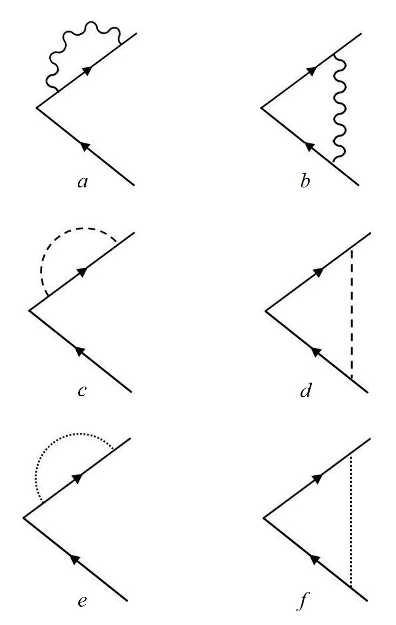
Figure 2: $(a,b)$ the $1/N$ contribution to $z^{\dagger}\sigma^{1,2}z$ and $\bar{\psi}\tau^{1,2}\psi$ from the gauge field fluctuation, the solid lines represent either the propagator of $z_{\alpha}$ or $\psi_{\alpha}$, the wavy line represents the propagator of the photon; $(c,d)$ the $1/N$ contribution to $z^{\dagger}\vec{\sigma}z$ from $\lambda_{\pm}$ in Eq. 17; $(e,f)$ the contribution to $B$ in Eq. 18.

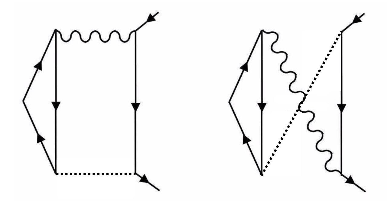
Figure 3: The two diagrams at $g_{v}^{3}$ order which cancel each other for arbitrary gauge choices.

The schematic beta function of $g_{v}$ reads

$$\frac{dg_{v}}{d\ln l}=(1-\Delta_{v})g_{v}-Bg_{v}^{3}+O(v^{5}).$$ (18)

$\Delta_{v}$ is the scaling dimension of $z^{\dagger}_{j}\vec{\sigma}z_{j}$ in the large$-N$ generalization of the EP-NCCP¹ model Eq. 11, with $\vec{\sigma}=(\sigma^{1},\sigma^{2})$. The standard $1/N$ calculation leads to

$$\Delta_{v}=1-\frac{56}{3\pi^{2}N}+O(\frac{1}{N^{2}}).$$ (19)

The $1/N$ correction of $\Delta_{v}$ comes from diagram Fig. 2$(a-d)$, where the wavy line is the gauge boson propagator, and the dashed line represents propagators of both $\lambda_{\pm}$. The first term of Eq. 19 implies that $g_{v}$ is indeed weakly relevant with finite but large$-N$.

The constant $B$ in the beta function arises from the operator product expansion of the coupling term Eq. 13, which is equivalent to the diagrams Fig. 2$e,f$. This computation leads to $B=1/(3\pi^{2})$. The two diagrams in Fig. 3 which are also at $g_{v}^{3}$ order cancel each other for arbitrary gauge choices. Similar two-loop diagrams at the same order of $1/N$ do not enter the RG equation due to lack of logarithmic contribution, as was explained in Ref. Benvenuti and Khachatryan, 2019. $\vec{\Phi}$ does not receive a wave function renormalization due to the singular form of its action. Hence with finite but large$-N$, $g_{v}$ indeed flows to a new fixed point:

$$g_{v\ast}^{2}=\frac{56}{N}+O(\frac{1}{N^{2}}).$$ (20)

We stress that this result is drawn from a controlled calculation and it is valid to the leading order of $1/N$.

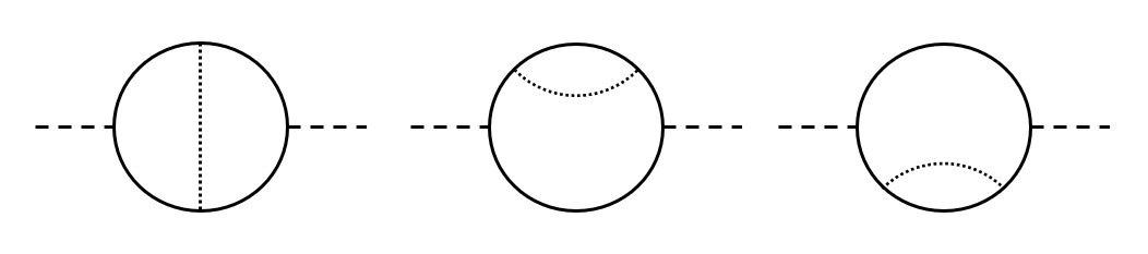
Figure 4: The $g_{v}^{2}$ diagrams that contributes to the scaling dimension of $[\lambda_{+}]$. Here the solid line represents the propagator of $z_{j,\alpha}$, the dotted line represents the vector operator $\vec{\Phi}$, and the dashed line represents $\lambda_{+}$.

As we explained before, the point $r=0$ is a direct transition between two ordered phases that spontaneously break the two ${\rm U}(1)$ symmetries. This transition will be driven to a new fixed point by coupling to the boundary fluctuations of bulk critical points as we demonstrated above. At this new fixed point, the critical exponent $\nu$ follows from the relation

$$\nu^{-1}=3-[\lambda_{+}].$$ (21)

To evaluate the scaling dimension $[\lambda_{+}]$ we have to incorporate the contributions of $g_{v}^{2}$ from the diagrams shown in Fig. 4, and combined with $1/N$ calculations performed previously Wen and Wu (1993); Benvenuti and Khachatryan (2019). Then in the end we obtain

$$\nu^{-1}_{*} = 1+\frac{160}{3\pi^{2}N}+\frac{4g_{v*}^{2}}{3\pi^{2}}+O(\frac{1}{N^{2}})$$ (22)

$$= 1+\frac{128}{\pi^{2}N}+O(\frac{1}{N^{2}}).$$ (24)

Again, there are other loop diagrams which appear to be at the same order of $1/N$ but do not make any logarithmic contributions Benvenuti and Khachatryan (2019).

III Interface States Embedded in $3d$ bulk

III.1 Interface states of noninteracting electron systems

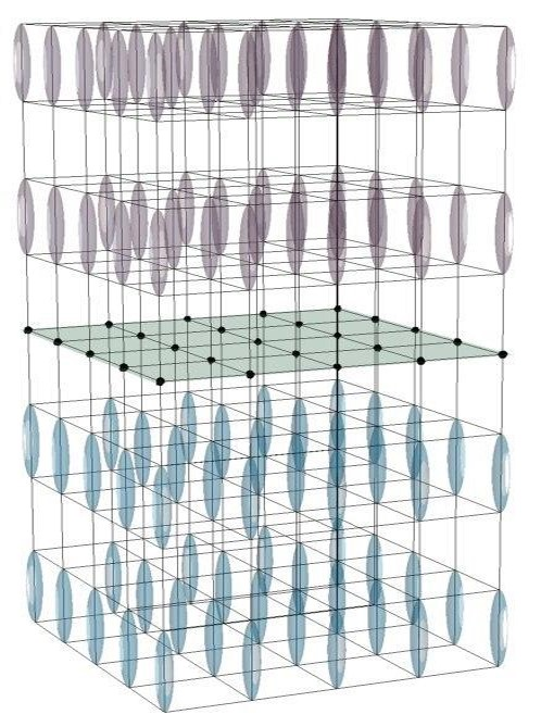
Figure 5: We consider a ${\rm SU}(N)$ antiferromagnet with self-conjugate representation on each site. The system forms a background VBS pattern, with opposite dimerizations between semi-infinite spaces $z>0$ and $z<0$. There is a $2d$ antiferromagnet localized at the interface $z=0$, and the entire bulk can undergo phase transition simultaneously due to the mirror (reflection) symmetry that connects the two sides of the domain wall.

In previous examples we studied topological edge states at the boundary of a $3d$ system. In this section we will consider the $2d$ states localized at an interface ($z=0$) in a $3d$ space, when the entire $3d$ bulk (for both $z>0$ and $z<0$ semi-infinite spaces) undergoes a phase transition simultaneously. Without fine-tuning, we need to assume an extra reflection symmetry $z\rightarrow-z$ that connects the two sides of the interface, which guarantees a simultaneous phase transition in the entire system. In this case there is no physical reason to impose the strong boundary condition at the interface embedded in the $3d$ space, hence the quantum critical modes at the interface follow the ordinary bulk scalings, instead of the weakened correlation of boundary CFT.

Again we will consider free fermion systems first. Let us first recall that the AIII class TI has a $\mathbb{Z}$ classification which is characterized by a topological index $n_{T}$. $n_{T}$ will appear as the coefficient of the electromagnetic response of the TI: $\mathcal{L}\sim i\pi n_{T}\mathbf{E}\cdot\mathbf{B}$. $n_{T}$ must change sign under spatial reflection transformation $\mathcal{M}_{z}:z\rightarrow-z$. To construct the desired system, we assume the semi-infinite space $z<0$ is occupied with the AIII class TI with Hamiltonian $\hat{H}$, whose topological index is $n_{T}$; and its “reflection conjugate” $\mathcal{M}_{z}^{-1}\hat{H}\mathcal{M}_{z}$ fills the semi-infinite space $z>0$. Then there are $N_{f}=2n_{T}$ flavors of massless Dirac fermions localized at the $2d$ plane $z=0$, which are still protected by time-reversal symmetry. Now we assume the entire bulk undergoes a quantum phase transition with a spontaneous time-reversal symmetry breaking, whose order parameter couples to the domain wall Dirac fermions as

$$\mathcal{S} = \int d^{2}xd\tau\ \sum_{\alpha=1}^{N_{f}}\bar{\psi}_{\alpha}\gamma_{\mu}\partial_{\mu}\psi_{\alpha}+g\phi\bar{\psi}_{\alpha}\psi_{\alpha}$$ (25)

$$+ \frac{1}{2}\phi(-\partial^{2})^{1/2}\phi.$$ (27)

The last term in the action is still defined in the $(2+1)d$ interface, and it reproduces the correlation of $\phi$ in the bulk: $\langle\phi(0)\phi(r)\rangle\sim 1/r^{2}$. We stress that, since now the order parameter resides in the entire bulk, $\phi$ no longer obeys the boundary scaling as we discussed in previous examples. A negative boson mass term $-r\phi^{2}$ can be generated through the standard fermion mass loop diagram, hence we need to tune an extra term at the interface to make sure the mass term of $\phi$ vanishes.

In this case the coupling constant $g$ is a marginal perturbation based on simple power-counting. But $g$ will flow under renormalization group (RG) with loop corrections in Fig. 2$(e,f)$:

$$\beta(g)=\frac{dg}{d\ln l}=-\frac{2}{3\pi^{2}}g^{3}+O(g^{5}).$$ (28)

Hence even in this case, the coupling between the domain wall states and the bulk quantum critical modes is perturbatively marginally irrelevant.

So far we have assumed that the velocity of the interface state is identical with the bulk. Now let us tune the velocity of the domain wall Dirac fermions slightly different, which can be captured by the following term in the Lagrangian:

$$\sum_{\alpha}\delta\bar{\psi}_{\alpha}(\gamma^{1}\partial_{x}+\gamma^{2}\partial_{y}-2\gamma^{3}\partial_{3})\psi_{\alpha}.$$ (29)

$\delta$ defined above is an eigenvector under the leading order RG flow. With the loop diagrams in Fig. 6, we obtain the leading order beta function of $\delta$:

$$\beta(\delta)=\frac{d\delta}{d\ln l}=-\frac{1}{5\pi^{2}}g^{2}\delta.$$ (30)

Together with $\beta(g)$, the velocity anisotropy is also perturbatively irrelevant.

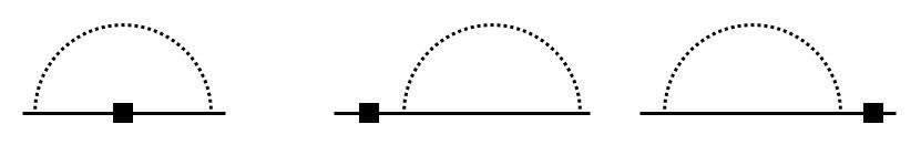
Figure 6: The Feynman diagrams that renormalizes the extra velocity $\delta$ in Eq. 29. The box represents the vertex $\delta$, and all three diagrams contributes to the fermion self-energy and renormalize $\delta$.

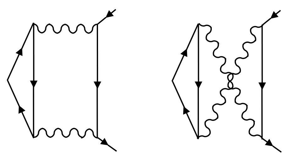
Figure 7: The extra diagrams that contribute to the scaling dimension of $\sum_{\alpha}\bar{\psi}_{\alpha}\psi_{\alpha}$ at the leading order of $1/N_{f}$ in QED₃. Again the wavy lines are photon propagators.

III.2 Interface states of quantum antiferromagnet

We now consider a ${\rm SU}(N)$ quantum antiferromagnet on a tetragonal lattice with a self-conjugate representation on each site (we assume $N$ is an even integer). With large$-N$, an antiferromagentic Heisenberg ${\rm SU}(N)$ model has a dimerized ground state Rokhsar (1990); Read and Sachdev (1989) where the two ${\rm SU}(N)$ spins on two nearest neighbor sites form a spin singlet (valence bond). We consider the following background configuration of valence bond solid (VBS): the spins form VBS along the $\hat{z}$ direction which spontaneously break the translation symmetry, while there is a domain wall between two opposite dimerizations at the $2d$ XY plane $z=0$, namely $z=0$ is still a mirror plane of the system (Fig. 5). In each $1d$ chain along the $\hat{z}$ direction, there is a dangling self-conjugate ${\rm SU}(N)$ spin localized on the site at the domain wall. Hence the $2d$ domain wall is effectively a ${\rm SU}(N)$ antiferromagnet on a square lattice.

One state of ${\rm SU}(N)$ antiferromagnet which is the “parent” state of many orders and topological orders on the square lattice, is the gapless $\pi-$flux ${\rm U}(1)$ spin liquid Affleck and Marston (1988); Hermele et al. (2005). At low energy this spin liquid is described by the following action of $(2+1)d$ quantum electrodynamics (QED₃):

$$\mathcal{S}=\int d^{2}xd\tau\ \sum_{\alpha=1}^{N_{f}}\bar{\psi}_{\alpha}\gamma_{\mu}(\partial_{\mu}-\mathrm{i}a_{\mu})\psi_{\alpha}+\cdots$$ (31)

$\psi_{\alpha}$ is $N_{f}=2N$ flavors of $2-$component Dirac fermions, and they are the low energy Dirac fermion modes of the slave fermion $f_{j,\alpha}$ defined as $\hat{S}^{b}_{j}=f^{\dagger}_{j,\alpha}T^{b}_{\alpha\beta}f_{j,\beta}$, $T^{b}$ with $b=1\cdots N^{2}-1$ are the fundamental representation of the ${\rm SU}(N)$ Lie Algebra. Besides the spin components, there is an extra two dimensional internal space which corresponds to two Dirac points in the Brillouin zone. There is an emergent ${\rm SU}(N_{f})$ flavor symmetry in QED₃ which includes both the ${\rm SU}(N)$ spin symmetry and discrete lattice symmetry.

It is known that when $N_{f}$ is greater than a critical integer, the QED₃ is a conformal field theory (CFT). We will consider the fate of this CFT when the three dimensional bulk is driven to a quantum phase transition. We will first consider a disorder-to-order quantum phase transition, where the ordered phase spontaneously breaks the time-reversal and parity symmetry of the XY plane. Notice that due to the reflection symmetry $z\rightarrow-z$ of the background VBS configuration, the two sides of the domain wall will reach the quantum critical point simultaneously. The bulk transition is still described by Eq. 2. When we couple the Ising order parameter $\phi$ to the domain wall QED₃, the total $(2+1)d$ action reads

$$\mathcal{S} = \int d^{2}xd\tau\ \sum_{\alpha=1}^{N_{f}}\bar{\psi}_{\alpha}\gamma_{\mu}(\partial_{\mu}-\mathrm{i}a_{\mu})\psi_{\alpha}$$ (32)

$$+ g\phi\bar{\psi}_{\alpha}\psi_{\alpha}+\frac{1}{2}\phi(-\partial^{2})^{1/2}\phi.$$ (34)

If the gauge field fluctuation is ignored, or equivalently in the large$-N_{f}$ limit, the scaling dimension of $\bar{\psi}\psi$ is $[\bar{\psi}\psi]=2$, and hence the scaling dimension of $g$ is $[g]=0$, $i.e.$ $g$ is a marginal perturbation. The $1/N_{f}$ correction to the RG flow arises from the Feynman diagrams (Fig. 2$(a,b)$ and Fig. 7) which involves one or two photon propagators:

$$G^{a}_{\mu\nu}(\vec{p})=\frac{16}{N_{f}p}\left(\delta_{\mu\nu}-\frac{p_{\mu}p_{\nu}}{p^{2}}\right).$$ (35)

Again in this case the fermions will generate a mass term for the order parameter at the interface, which we need to tune to zero. At the leading order of $1/N_{f}$ the corrected beta function for $g$ reads

$$\beta(g)=\frac{dg}{d\ln l}=-\frac{128}{3\pi^{2}N_{f}}g-\frac{2}{3\pi^{2}}g^{3}+O(g^{3}).$$ (36)

But this beta function does not lead to a new unitary fixed point other than the decoupled fixed point $g=0$. Hence in this case the domain wall state is decoupled from the bulk quantum critical modes in the infrared limit.

A more interesting scenario is when the bulk undergoes a transition which spontaneously breaks the translation and $C_{4}$ rotation symmetry by developing an extra VBS order within the XY plane. The inplane VBS order parameters are $V_{x}\sim\bar{\psi}\tau^{1}\psi$, and $V_{y}\sim\bar{\psi}\tau^{2}\psi$, where $\tau^{1,2}$ are the Pauli matrices operating in the Dirac valley space. The coupling between the VBS order parameter and the domain wall QED₃ reads

$$\mathcal{S}_{c}=\int d^{2}xd\tau\ g\left(\phi^{\ast}\bar{\psi}\tau^{-}\psi+\phi\bar{\psi}\tau^{+}\psi\right)+\phi^{\ast}(-\partial^{2})^{1/2}\phi.$$ (37)

Here $\tau^{\pm}=(\tau^{1}\pm\mathrm{i}\tau^{2})/2$. The scaling dimension of the VBS order parameter at the QED₃ fixed point has been computed previously Hermele et al. (2005); Rantner and Wen (2001); Xu and Sachdev (2008): $[\bar{\psi}\tau^{a}\psi]=2-64/(3\pi^{2}N_{f})$, and the beta function of $g$ to the leading order of $1/N_{f}$ reads

$$\beta(g)=\frac{64}{3\pi^{2}N_{f}}g-\frac{1}{6\pi^{2}}g^{3}+O(g^{3}).$$ (38)

In the large$-N_{f}$ limit, the coupling $g$ is marginally irrelevant; but with finite and large$-N_{f}$, $g$ is weakly relevant at the noninteracting fixed point, and it will flow to an interacting fixed point

$$g_{\ast}^{2}=\frac{128}{N_{f}}+O(\frac{1}{N_{f}^{2}}).$$ (39)

This new fixed point will break the emergent ${\rm SU}(N_{f})$ flavor symmetry down to ${\rm SU}(N)\times U(1)$ symmetry, where ${\rm U}(1)$ corresponds to the rotation of the Dirac valley space. The following gauge invariant operators receive different corrections to their scaling dimensions from coupling to the bulk quantum critical modes:

$$[\bar{\psi}\psi] = 2+\frac{128}{3\pi^{2}N_{f}}+\frac{2}{3\pi^{2}}g_{\ast}^{2}+O(\frac{1}{N_{f}^{2}});$$ (40)

$$[\bar{\psi}T^{b}\psi] = 2-\frac{64}{3\pi^{2}N_{f}}+\frac{2}{3\pi^{2}}g_{\ast}^{2}+O(\frac{1}{N_{f}^{2}});$$ (42)

$$[\bar{\psi}\tau^{3}\psi] = 2-\frac{64}{3\pi^{2}N_{f}}-\frac{1}{3\pi^{2}}g_{\ast}^{2}+O(\frac{1}{N_{f}^{2}});$$ (44)

$$[\bar{\psi}\tau^{1,2}\psi] = 2-\frac{64}{3\pi^{2}N_{f}}+\frac{1}{6\pi^{2}}g_{\ast}^{2}.$$ (46)

The operators $\bar{\psi}\tau^{1,2}\psi$ have exactly scaling dimension 2, the Feynman diagram contributions from Fig. 2 cancel each other for operator $\bar{\psi}\tau^{1,2}\psi$ as they should. Notice that the last three operators in Eq. 46 should have the same scaling dimension in the original QED₃ fixed point due to the large ${\rm SU}(N_{f})$ flavor symmetry, but at this new fixed point they will acquire different corrections.

Another interesting scenario is that the bulk is at a critical point whose order parameter couples to the Ising like operator $\bar{\psi}\tau^{3}\psi$, which breaks the inplane parity but preserves the time-reversal:

$$\mathcal{S}_{c}=\int d^{2}xd\tau\ g\phi\bar{\psi}\tau^{3}\psi+\frac{1}{2}\phi(-\partial^{2})^{1/2}\phi.$$ (47)

The microsopic representation of the operator $\bar{\psi}\tau^{3}\psi$ can be found in Ref. Hermele et al., 2005. The beta function of the coupling $g$ reads

$$\beta(g)=\frac{64}{3\pi^{2}N_{f}}g-\frac{2}{3\pi^{2}}g^{3}+O(g^{3}),$$ (48)

and once again there is new stable fixed point $g_{\ast}^{2}=32/N_{f}+O(1/N_{f}^{2})$. And at this fixed point,

$$[\bar{\psi}\psi] = 2+\frac{128}{3\pi^{2}N_{f}}+\frac{2}{3\pi^{2}}g_{\ast}^{2}+O(\frac{1}{N_{f}^{2}});$$ (49)

$$[\bar{\psi}T^{b}\psi] = 2-\frac{64}{3\pi^{2}N_{f}}+\frac{2}{3\pi^{2}}g_{\ast}^{2}+O(\frac{1}{N_{f}^{2}});$$ (51)

$$[\bar{\psi}\tau^{1,2}\psi] = 2-\frac{64}{3\pi^{2}N_{f}}-\frac{1}{3\pi^{2}}g_{\ast}^{2}+O(\frac{1}{N_{f}^{2}});$$ (53)

$$[\bar{\psi}\tau^{3}\psi] = 2-\frac{64}{3\pi^{2}N_{f}}+\frac{2}{3\pi^{2}}g_{\ast}^{2}.$$ (55)

The domain wall state considered here is formally equivalent to the boundary state of a $3d$ bosonic SPT state with pSU$(N)\times{\rm U}(1)$ symmetry, which can also be embedded to the $3d$ SPT with pSU($N_{f}$) symmetry discussed in Ref. Xu, 2013. This SPT state can be constructed as follows: we first break the ${\rm U}(1)$ symmetry in the $3d$ bulk by driving the bulk $z<0$ into a superfluid phase, and then decorate the vortex loop of the superfluid phase with a $1d$ Haldane phase with pSU$(N)$ symmetry Nonne et al. (2013); Bois et al. (2015); Capponi et al. (2016); Duivenvoorden and Quella (2013). Eventually we proliferate the decorated vortex loops to restore all the symmetries in the bulk. A $1d$ pSU$(N)$ Haldane phase can be constructed as a spin-chain with a pSU$(N)$ spin on each site, and there is a dangling self-conjugate representation of ${\rm SU}(N)$ on each end of the chain. And this dangling spin will also exist in the ${\rm U}(1)$ vortex at the boundary of the pSU$(N)\times{\rm U}(1)$ SPT state. Notice that the self-conjugate representation of ${\rm SU}(N)$ is a projective representation of pSU($N$).

IV Discussion

In this work we systematically studied the interplay of two different nontrivial boundary effects: the $2d$ edge states of $3d$ symmetry protected topological states, and the boundary fluctuations of $3d$ bulk quantum phase transitions. New fixed points were identified through generic field theory descriptions of these systems and controlled calculations. We then generalized our study to the $2d$ states localized at the interface embedded in the $3d$ bulk.

The last case studied in Eq. 48, 55 is special when $N_{f}=2$, and when the gauge field is noncompact. This is the theory that has been shown to be dual to the EP-NCCP¹ model Potter et al. (2017); Wang et al. (2017) studied in Eq. 8, the operator $\sum_{\alpha}r|z_{\alpha}|^{2}$ is dual to $r\bar{\psi}\tau^{3}\psi$, and both theories are self-dual. By coupling the operator $\bar{\psi}\tau^{3}\psi$ to the bulk critical modes (rather than the boundary fluctuations of the bulk critical points), we have shown that this $(2+1)d$ theory is driven to a new fixed point, and the self-duality structure still holds. The self-duality transformation of Eq. 8 now is combined with the Ising symmetry of the order parameter $\phi$. However, the $\mathrm{O}(4)$ emergent symmetry no longer exists at this new fixed point, due to the nonzero fixed point of $g$ in Eq. 47.

The methodology used in this work can have many potential extensions. We can apply the same field theory and RG calculation to the $1d$ boundary of $2d$ SPT states (for instance the AKLT state), which was studied through exactly soluble lattice Hamiltonians Scaffidi et al. (2017) and also numerical methods Zhang and Wang (2017); Weber et al. (2018); Weber and Wessel (2019). Also, $1d$ defect in a $3d$ topological state can also have gapless modes Ran et al. (2009); Teo and Kane (2010), it would be interesting to investigate the fate of a $1d$ defect embedded in a $3d$ bulk at the bulk quantum phase transition. Defects of free or weakly interacting fermionic topological insulator and topological superconductor coupled with bulk critical modes was studied in Ref. Grover and Vishwanath, 2012, but we expect the defect of an intrinsic strongly interacting topological state can lead to much richer physics. Last but not least, the “higher order topological insulator” has nontrivial modes localized at the corner instead of the boundary of the system Benalcazar et al. (2017). The coupling between the bulk quantum critical points and corner topological modes is also worth exploration.

This work is supported by NSF Grant No. DMR-1920434, the David and Lucile Packard Foundation, and the Simons Foundation. The authors thank Andreas Ludwig and Leon Balents for helpful discussions.

References

- Kane and Mele (2005a) C. L. Kane and E. J. Mele, Physical Review Letter 95, 226801 (2005a).
- Kane and Mele (2005b) C. L. Kane and E. J. Mele, Physical Review Letter 95, 146802 (2005b).
- Fu et al. (2008) L. Fu, C. L. Kane, and E. J. Mele, Phys. Rev. Lett. 98, 106803 (2008).
- Moore and Balents (2007) J. E. Moore and L. Balents, Phys. Rev. B 75, 121306(R) (2007).
- Schnyder et al. (2009) A. P. Schnyder, S. Ryu, A. Furusaki, and A. W. W. Ludwig, AIP Conf. Proc. 1134, 10 (2009).
- Ryu et al. (2010) S. Ryu, A. Schnyder, A. Furusaki, and A. Ludwig, New J. Phys. 12, 065010 (2010).
- Kitaev (2009) A. Kitaev, AIP Conf. Proc 1134, 22 (2009).
- Chen et al. (2013) X. Chen, Z.-C. Gu, Z.-X. Liu, and X.-G. Wen, Phys. Rev. B 87, 155114 (2013).
- Chen et al. (2012) X. Chen, Z.-C. Gu, Z.-X. Liu, and X.-G. Wen, Science 338, 1604 (2012).
- Fidkowski et al. (2013) L. Fidkowski, X. Chen, and A. Vishwanath, Phys. Rev. X 3, 041016 (2013).
- Chen et al. (2014) X. Chen, L. Fidkowski, and A. Vishwanath, Phys. Rev. B 89, 165132 (2014).
- Bonderson et al. (2013) P. Bonderson, C. Nayak, and X.-L. Qi, J. Stat. Mech. p. P09016 (2013).
- Wang et al. (2013) C. Wang, A. C. Potter, and T. Senthil, Phys. Rev. B 88, 115137 (2013).
- Metlitski et al. (2013) M. A. Metlitski, C. L. Kane, and M. P. A. Fisher, arXiv:1306.3286 (2013).
- Wang and Senthil (2013) C. Wang and T. Senthil, Phys. Rev. B 87, 235122 (2013).
- Cheng et al. (2016) M. Cheng, M. Zaletel, M. Barkeshli, A. Vishwanath, and P. Bonderson, Phys. Rev. X 6, 041068 (2016), URL https://link.aps.org/doi/10.1103/PhysRevX.6.041068.
- Vishwanath and Senthil (2013) A. Vishwanath and T. Senthil, Phys. Rev. X 3, 011016 (2013).
- Xu and You (2015) C. Xu and Y.-Z. You, Phys. Rev. B 92, 220416 (2015), URL https://link.aps.org/doi/10.1103/PhysRevB.92.220416.
- Mross et al. (2016) D. F. Mross, J. Alicea, and O. I. Motrunich, Phys. Rev. Lett. 117, 016802 (2016), URL https://link.aps.org/doi/10.1103/PhysRevLett.117.016802.
- Hsin and Seiberg (2016) P.-S. Hsin and N. Seiberg, Journal of High Energy Physics 2016, 95 (2016), ISSN 1029-8479, URL http://dx.doi.org/10.1007/JHEP09(2016)095.
- Wang et al. (2017) C. Wang, A. Nahum, M. A. Metlitski, C. Xu, and T. Senthil, Phys. Rev. X 7, 031051 (2017), URL https://link.aps.org/doi/10.1103/PhysRevX.7.031051.
- Seiberg et al. (2016) N. Seiberg, T. Senthil, C. Wang, and E. Witten, Annals of Physics 374, 395 (2016), ISSN 0003-4916, URL http://www.sciencedirect.com/science/article/pii/S00034916163%01531.
- Senthil et al. (2019) T. Senthil, D. T. Son, C. Wang, and C. Xu, Physics Reports 827, 1 (2019), ISSN 0370-1573, duality between (2+1)d quantum critical points, URL http://www.sciencedirect.com/science/article/pii/S03701573193%02637.
- Cardy (1996) J. Cardy, Scaling and Renormalization in Statistical Physics (Cambridge Lecture Notes in Physics, 1996).
- Cardy (1984) J. L. Cardy, Nuclear Physics B 240, 514 (1984), ISSN 0550-3213, URL http://www.sciencedirect.com/science/article/pii/055032138490%2414.
- Dietrich and Diehl (1983) S. Dietrich and H. W. Diehl, Zeitschrift für Physik B Condensed Matter 51, 343 (1983), ISSN 1431-584X, URL https://doi.org/10.1007/BF01319217.
- Diehl and Dietrich (1981) H. W. Diehl and S. Dietrich, Zeitschrift für Physik B Condensed Matter 42, 65 (1981), ISSN 1431-584X, URL https://doi.org/10.1007/BF01298293.
- Reeve and Guttmann (1981) J. Reeve and A. J. Guttmann, Journal of Physics A: Mathematical and General 14, 3357 (1981), URL https://doi.org/10.1088%2F0305-4470%2F14%2F12%2F028.
- Diehl (1997) H. W. Diehl, International Journal of Modern Physics B 11, 3503 (1997), eprint https://doi.org/10.1142/S0217979297001751, URL https://doi.org/10.1142/S0217979297001751.
- Scaffidi et al. (2017) T. Scaffidi, D. E. Parker, and R. Vasseur, Phys. Rev. X 7, 041048 (2017), URL https://link.aps.org/doi/10.1103/PhysRevX.7.041048.
- Verresen et al. (2018) R. Verresen, N. G. Jones, and F. Pollmann, Phys. Rev. Lett. 120, 057001 (2018), URL https://link.aps.org/doi/10.1103/PhysRevLett.120.057001.
- Verresen et al. (2019) R. Verresen, R. Thorngren, N. G. Jones, and F. Pollmann, arXiv e-prints arXiv:1905.06969 (2019), eprint 1905.06969.
- Zhang and Wang (2017) L. Zhang and F. Wang, Phys. Rev. Lett. 118, 087201 (2017), URL https://link.aps.org/doi/10.1103/PhysRevLett.118.087201.
- Weber et al. (2018) L. Weber, F. Parisen Toldin, and S. Wessel, Phys. Rev. B 98, 140403 (2018), URL https://link.aps.org/doi/10.1103/PhysRevB.98.140403.
- Weber and Wessel (2019) L. Weber and S. Wessel, Phys. Rev. B 100, 054437 (2019), URL https://link.aps.org/doi/10.1103/PhysRevB.100.054437.
- Grover and Vishwanath (2012) T. Grover and A. Vishwanath, arXiv e-prints arXiv:1206.1332 (2012), eprint 1206.1332.
- Bi et al. (2015) Z. Bi, A. Rasmussen, K. Slagle, and C. Xu, Phys. Rev. B 91, 134404 (2015), URL https://link.aps.org/doi/10.1103/PhysRevB.91.134404.
- Motrunich and Vishwanath (2004) O. I. Motrunich and A. Vishwanath, Phys. Rev. B 70, 075104 (2004).
- Senthil et al. (2004a) T. Senthil, A. Vishwanath, L. Balents, S. Sachdev, and M. P. A. Fisher, Science 303, 1490 (2004a).
- Senthil et al. (2004b) T. Senthil, L. Balents, S. Sachdev, A. Vishwanath, and M. P. A. Fisher, Phys. Rev. B 70, 144407 (2004b).
- Potter et al. (2017) A. C. Potter, C. Wang, M. A. Metlitski, and A. Vishwanath, Phys. Rev. B 96, 235114 (2017), URL https://link.aps.org/doi/10.1103/PhysRevB.96.235114.
- Kaul and Sachdev (2008) R. K. Kaul and S. Sachdev, Phys. Rev. B 77, 155105 (2008), URL https://link.aps.org/doi/10.1103/PhysRevB.77.155105.
- Benvenuti and Khachatryan (2019) S. Benvenuti and H. Khachatryan, Journal of High Energy Physics 2019, 214 (2019), ISSN 1029-8479, URL https://doi.org/10.1007/JHEP05(2019)214.
- Wen and Wu (1993) X.-G. Wen and Y.-S. Wu, Phys. Rev. Lett. 70, 1501 (1993), URL https://link.aps.org/doi/10.1103/PhysRevLett.70.1501.
- Rokhsar (1990) D. S. Rokhsar, Phys. Rev. B 42, 2526 (1990), URL https://link.aps.org/doi/10.1103/PhysRevB.42.2526.
- Read and Sachdev (1989) N. Read and S. Sachdev, Nuclear Physics B 316, 609 (1989), ISSN 0550-3213, URL http://www.sciencedirect.com/science/article/pii/055032138990%0618.
- Affleck and Marston (1988) I. Affleck and J. B. Marston, Phys. Rev. B 37, 3774 (1988), URL https://link.aps.org/doi/10.1103/PhysRevB.37.3774.
- Hermele et al. (2005) M. Hermele, T. Senthil, and M. P. A. Fisher, Phys. Rev. B 72, 104404 (2005).
- Rantner and Wen (2001) W. Rantner and X.-G. Wen, Phys. Rev. Lett. 86, 3871 (2001), URL https://link.aps.org/doi/10.1103/PhysRevLett.86.3871.
- Xu and Sachdev (2008) C. Xu and S. Sachdev, Phys. Rev. Lett. 100, 137201 (2008), URL https://link.aps.org/doi/10.1103/PhysRevLett.100.137201.
- Xu (2013) C. Xu, Phys. Rev. B 87, 144421 (2013).
- Nonne et al. (2013) H. Nonne, M. Moliner, S. Capponi, P. Lecheminant, and K. Totsuka, EPL (Europhysics Letters) 102, 37008 (2013), URL http://stacks.iop.org/0295-5075/102/i=3/a=37008.
- Bois et al. (2015) V. Bois, S. Capponi, P. Lecheminant, M. Moliner, and K. Totsuka, Phys. Rev. B 91, 075121 (2015), URL https://link.aps.org/doi/10.1103/PhysRevB.91.075121.
- Capponi et al. (2016) S. Capponi, P. Lecheminant, and K. Totsuka, Annals of Physics 367, 50 (2016), ISSN 0003-4916, URL http://www.sciencedirect.com/science/article/pii/S00034916160%00130.
- Duivenvoorden and Quella (2013) K. Duivenvoorden and T. Quella, Phys. Rev. B 87, 125145 (2013), URL http://link.aps.org/doi/10.1103/PhysRevB.87.125145.
- Ran et al. (2009) Y. Ran, Y. Zhang, and A. Vishwanath, Nature Physics 5, 298 (2009).
- Teo and Kane (2010) J. C. Y. Teo and C. L. Kane, Phys. Rev. B 82, 115120 (2010), URL https://link.aps.org/doi/10.1103/PhysRevB.82.115120.
- Benalcazar et al. (2017) W. A. Benalcazar, B. A. Bernevig, and T. L. Hughes, Science 357, 61 (2017), ISSN 0036-8075, eprint https://science.sciencemag.org/content/357/6346/61.full.pdf, URL https://science.sciencemag.org/content/357/6346/61.