Anomaly Inflow Methods for SCFT Constructions in Type IIB

Abstract

We extend the anomaly inflow methods developed in M-theory to SCFTs engineered via D3-branes in type IIB. We show that the ’t Hooft anomalies of such SCFTs can be computed systematically from their geometric definition. Our procedure is tested in several 4d examples and applied to 2d theories obtained by wrapping D3-branes on a Riemann surface. In particular, we show how to analyze half-BPS regular punctures for 4d $\mathcal{N}=4$ SYM on a Riemann surface. We discuss generalizations of this formalism to type IIB configurations with $F_{3}$, $H_{3}$ fluxes, as well as to F-theory setups.

1 Introduction

Geometric engineering is a powerful tool in the construction and analysis of quantum field theories (QFTs) in various dimensions. In many situations, geometric methods in string/M-/F-theory allow one to study strongly coupled QFTs for which a Lagrangian description is not available. A prototypical example is furnished by 4d QFTs obtained by wrapping M5-branes on a Riemann surface with punctures, preserving $\mathcal{N}=2$ Gaiotto:2009we ; Gaiotto:2009hg or $\mathcal{N}=1$ Maruyoshi:2009uk ; Benini:2009mz ; Bah:2011je ; Bah:2011vv ; Bah:2012dg supersymmetry.

’t Hooft anomalies are among the most interesting quantities to compute in a geometrically engineered theory. Since ’t Hooft anomalies are invariant under RG flow, they are particularly robust observables and can be used to constrain the phases of theories in a non-perturbative way. In this work, we focus on ’t Hooft anomalies for continuous 0-form symmetries. These anomalies only occur for QFT in even $d$ spacetime dimensions, and are conveniently summarized in the anomaly polynomial, which is a $(d+2)$-form characteristic class constructed with the curvatures of the background fields that couple to the global symmetries.

In Bah:2018gwc ; Bah:2018jrv ; Bah:2019jts ; Bah:2019rgq ; Bah:2019vmq systematic tools have been developed to compute the anomaly polynomial for even-dimensional QFTs obtained from wrapped M5-branes. The methods of Bah:2018gwc ; Bah:2018jrv ; Bah:2019jts ; Bah:2019rgq ; Bah:2019vmq are based on the anomaly inflow mechanism for M5-branes, first studied in Duff:1995wd ; Witten:1996hc ; Freed:1998tg ; Harvey:1998bx . The main strategy underlying these inflow-based tools is to shift the focus from the worldvolume theory on the M5-branes to the supergravity fields in 11d ambient space that surrounds the branes. In the presence of the M5-brane stack, the supergravity fields acquire non-trivial boundary conditions, which in turn generate a classical anomalous variation of the 11d effective action. This classical variation counterbalances the quantum anomalies of the worldvolume theory on the M5-branes (including anomalies of modes that decouple in the deep IR).

Having a systematic toolkit for the computation of anomalies in this class of theories is beneficial in various ways. For instance, the analysis of Bah:2018gwc ; Bah:2018jrv ; Bah:2019jts shows that the “bulk” and “puncture” contributions to ’t Hooft anomalies in a 4d $\mathcal{N}=2$ theory of class $\mathcal{S}$ with regular punctures can be treated on an equal footing. Indeed, both can be analyzed by studying the boundary conditions for the $G_{4}$-flux configuration near the M5-branes. Furthermore, the inflow perspective can be applied to holographic setups, where it has the potential of yielding finite terms in $N$ without resorting to AdS loop computations Bah:2019rgq . As exemplified in Bah:2019vmq , a careful treatment of the boundary conditions for the 11d supergravity fields can be efficiently used as a proxy to track non-trivial dynamics on the worldvolume of the branes, including the emergence of accidental symmetries and spontaneous symmetry breaking.

Given the success of anomaly inflow methods in M-theory, it is natural to ask whether similar tools can be developed for other string constructions. The main objective of this work is to formulate a proposal for inflow tools in type IIB string theory. In the M-theory case, an essential role is played by a formal 12-form $\mathcal{I}_{12}$, constructed with a 4-form $E_{4}$ that encodes the boundary condition for $G_{4}$ near the M5-branes. In the type IIB context, we have a formal 11-form $\mathcal{I}_{11}$, which is constructed with a 5-form $E_{5}$, and 3-forms $\mathcal{F}_{3}$, $\mathcal{H}_{3}$, which capture the boundary conditions for $F_{5}$, $F_{3}$, $H_{3}$, respectively. The structure of $\mathcal{I}_{11}$ is expected to be considerably richer if we upgrade from type IIB to F-theory (i.e. type IIB backgrounds in which the axio-dilaton profile has non-trivial monodromies around singular loci). We also comment about such extension, making contact with the constructions of Lawrie:2018jut .

To begin with, we consider setups with D3-branes in the absence of $F_{3}$, $H_{3}$ fluxes and with constant dilaton profile. These type IIB constructions have been studied intensively over the years. Typically, the worldvolume theory on the D3-branes is a well-understood Lagrangian theory. We may then use these setups to test our inflow methods. In particular, in these examples we have full control over the modes that decouple in the IR and we can explicitly verify that, keeping decoupling into account, anomaly inflow gives results that are exact in $N$ (the number of D3-branes in the stack). It is worth pointing out that recent work Fazzi:2019gvt demonstrates that there are still interesting aspects of the dynamics of D3-branes at the tip of a Calabi-Yau cone that are not fully understood and deserve further investigation. We propose that our inflow tools should be applicable to these less-understood cases, as well.

Next, we apply our inflow proposal to some 2d theories. In particular, we exploit the intuition developed in Bah:2018gwc ; Bah:2018jrv ; Bah:2019jts to compute the anomaly of 4d $\mathcal{N}=4$ SYM compactified on a Riemann surface with half-BPS punctures.

The rest of this paper is organized as follows. In section 2 we formulate our proposal for the computation of the inflow anomaly polynomial, introducing the main objects $E_{5}$, $\mathcal{F}_{3}$, $\mathcal{H}_{3}$, and $\mathcal{I}_{11}$. Section 3 is devoted to a careful study of several examples of 4d QFTs engineered using D3-branes in type IIB, which provide various checks of our proposal. In section 4 we consider some 2d examples, obtained from reduction from four dimensions on a Riemann surface without punctures, or with half-BPS punctures. Section 5 is dedicated to a preliminary investigation of the extension of $\mathcal{I}_{11}$ to F-theory setups. We conclude with a brief discussion. Some derivations and other technical material are collected in the appendices.

2 Inflow anomaly polynomial for type IIB

In this section we describe our proposal for the computation of the inflow anomaly polynomial for type IIB setups. A crucial role is played by a formal 11-form class $\mathcal{I}_{11}$, which captures the anomalous variation of the type IIB action in the presence of a boundary. Our method is inspired by the tools of Bah:2018gwc ; Bah:2018jrv ; Bah:2019jts ; Bah:2019rgq ; Bah:2019vmq for the analysis of anomaly inflow for M5-branes in M-theory. We therefore start with a quick review of M5-brane inflow before discussing our proposal for type IIB setups.

2.1 Review: anomaly inflow for M5-branes

Let us consider a stack of $N$ M5-branes with worldvolume $W_{6}$ inside the 11d spacetime $M_{11}$. We suppose that $W_{6}$ is of the form

$$W_{6}=W_{d}\times\mathcal{S}_{6-d}\ ,$$ (2.1)

where $W_{d}$ is external $d$-dimensional spacetime and $\mathcal{S}_{6-d}$ is a smooth compact internal space. The low-energy dynamics of the degrees of freedom localized at the stack furnishes a QFT in the $d$ external dimensions. We focus on the case of $d$ even. Our task is it exploit anomaly inflow from the 11d ambient space of M-theory to compute the ’t Hooft anomalies for global continuous symmetries of the QFT on $W_{d}$.

In order to specify the M5-brane configuration, we need both the geometry of the internal space $\mathcal{S}_{6-d}$, and information about the normal bundle $NW_{6}$ to the branes in the ambient 11d space. A convenient way to encode these data is to introduce a compact $(10-d)$-dimensional space $M_{10-d}$, which is an $S^{4}$ fibration over $\mathcal{S}_{6-d}$,

$$S^{4}\hookrightarrow M_{10-d}\rightarrow\mathcal{S}_{6-d}\ .$$ (2.2)

We think of the $S^{4}$ fiber as the unit sphere in the fibers of $NW_{6}$, or equivalently as the $S^{4}$ that surrounds the M5-brane stack in its five transverse directions. The fibering of $S^{4}$ over $\mathcal{S}_{6-d}$ encodes the partial topological twist of the 6d theory on $W_{6}$ compactified on $\mathcal{S}_{6-d}$.

The key observation for anomaly inflow in this setup is that the M5-brane stack acts as a singular magnetic source the M-theory flux $G_{4}$. Following Freed:1998tg ; Harvey:1998bx , the singularity is removed by excising a small tubular neighborhood of the M5-brane stack. As a result, the 11d spacetime $M_{11}$ acquires a boundary $\partial M_{11}=M_{10}$. If $r$ denotes the radial coordinate away from the M5-brane stack, $M_{10}$ is located at $r=\epsilon$, where $\epsilon$ is a small positive constant. The space $M_{10}$ is a fibration of $M_{10-d}$ over $W_{d}$,

$$M_{10-d}\hookrightarrow M_{10}\rightarrow W_{d}\ .$$ (2.3)

The fibering of the internal space $M_{10-d}$ over the external spacetime $W_{d}$ is due to the fact that we are turning on background gauge connections for the continuous global symmetries of the QFT living on $W_{d}$.

The magnetic source for $G_{4}$ is modeled by imposing suitable boundary conditions for $G_{4}$ near $r=\epsilon$. More precisely, we have Freed:1998tg ; Harvey:1998bx

$$\frac{G_{4}}{2\pi}=-\rho\,E_{4}+\dots\ .$$ (2.4)

In the above expression, $\rho$ is a bump function depending on $r$ only, which interpolates smoothly between $\rho=-1$ at $r=\epsilon$ and $\rho=0$ at large $r$. The ellipsis stands for terms with $dr$ legs and/or subleading terms in the limit $r\rightarrow\epsilon$. The quantity $E_{4}$ is a closed and globally-defined 4-form on $M_{10}$. (Thus, by definition, $E_{4}$ has no legs along $r$.) In order to be globally defined, $E_{4}$ must be gauge invariant under a gauge transformation of the external background gauge fields. Furthermore, the integral of $E_{4}$ along the $S^{4}$ fibers of $\mathcal{M}_{10-d}$, see (2.2), counts the total number of M5-branes in the stack,

$$\int_{S^{4}}E_{4}=N\ .$$ (2.5)

In the simplest situation in which we consider six uncompactified directions, the 4-form $E_{4}$ is given by

$$E_{4}=N\,e_{4}\qquad\text{(for $d=6$)}\ ,$$ (2.6)

where $e_{4}$ is the global angular form of $SO(5)$, normalized to integrate to 1 along $S^{4}$. The form $e_{4}$ is the $SO(5)$ invariant and closed completion of the volume form on $S^{4}$. Its expression can be found e.g. in Harvey:1998bx .

The boundary condition (2.4) for $G_{4}$ is used to build a formal 12-form characteristic class

$$\mathcal{I}_{12}=-\frac{1}{6}\,E_{4}^{3}-E_{4}\,X_{8}\ ,$$ (2.7)

where we suppressed wedge products for brevity, and we introduced the 8-form

$$X_{8}=\frac{1}{192}\bigg{[}p_{1}(TM_{11})^{2}-4\,p_{2}(TM_{11})\bigg{]}\ ,$$ (2.8)

where the quantities $p_{1,2}(TM_{11})$ are the first and second Pontryagin classes of the 11d tangent bundle, implicitly pulled back to the boundary at $r=\epsilon$. The importance of the 12-form $\mathcal{I}_{12}$ stems from the fact that it encodes the variation of the M-theory effective action in the presence of the boundary $M_{10}$. More precisely, the two terms in $\mathcal{I}_{12}$ originate from the Chern-Simons $C_{3}\,G_{4}\,G_{4}$ coupling and $C_{3}\,X_{8}$ coupling, respectively. The variation of the 11d action is related to $\mathcal{I}_{12}$ via standard descent procedure,

$$\mathcal{I}_{12}=d\mathcal{I}_{11}^{(0)}\ ,\qquad\delta\mathcal{I}_{11}^{(0)}=d\mathcal{I}_{10}^{(1)}\ ,\qquad\delta S_{\rm 11d}=2\pi\,\int_{M_{10}}\mathcal{I}_{10}^{(1)}\ .$$ (2.9)

As a result, the inflow anomaly polynomial for the worldvolume theory on $W_{d}$ is obtained by integrating $\mathcal{I}_{12}$ along the $M_{10-d}$ fibers of $M_{10}$, see (2.3),

$$I_{d+2}^{\rm inflow}=\int_{M_{10-d}}\mathcal{I}_{12}\ .$$ (2.10)

This quantity cancels against the ’t Hooft anomalies of all degrees of the freedom on $W_{d}$. We are mainly interested in the situation in which, at low energies, the worldvolume theory consists of an interacting CFT, together with decoupled fields. We may then write

$$I_{d+2}^{\rm inflow}+I_{d+2}^{\rm CFT}+I_{d+2}^{\rm decoupl}=0\ .$$ (2.11)

Uusually, one is interested in deriving $I_{d+2}^{\rm CFT}$. In this case, the quantity $I_{d+2}^{\rm decoupl}$ has to be identified and subtracted by hand from $I_{d+2}^{\rm inflow}$.

2.2 Inflow tools for D3-branes

We would like to develop a formalism analogous to the one of the previous section that can be applied to type IIB setups. For definiteness, we first consider a stack of $N$ D3-branes with worldvolume $W_{4}$ inside the spacetime $M_{10}$.

The stack supports localized degrees of freedom that yield a non-trivial QFT coupled to the 10d bulk. In the IR, it consists of $\mathcal{N}=4$ super Yang-Mills (SYM) with gauge group $SU(N)$, together with a free 4d $\mathcal{N}=4$ vector multiplet. The local Lorentz symmetry $SO(1,9)$ of type IIB is broken to $SO(1,3)\times SO(6)$, with $SO(1,3)$ identified with the local Lorentz symmetry of the worldvolume theory, and $SO(6)$ identified with its R-symmetry. (More precisely, the R-symmetry is $\text{Spin}(6)\cong SU(4)$.) The 4d worldvolume theory contains chiral degrees of freedom that induce a cubic ’t Hooft anomaly for the $SU(4)$ R-symmetry. Both the interacting SCFT and the decoupling modes admit a Lagrangian description, and the anomaly can be computed with standard methods. One has

$$I_{6}^{\rm CFT}=\frac{1}{2}\,(N^{2}-1)\,c_{3}(SU(4))\ ,\qquad I_{6}^{\rm decoupl}=\frac{1}{2}\,c_{3}(SU(4))\ ,\qquad$$ (2.12)

where $c_{3}$ denotes the third Chern class.

We expect that the anomaly (2.12) is counterbalanced by inflow from the type IIB bulk. This was indeed verified in Kim:2012wc by using the coupling $\int_{W_{4}}i^{*}C_{4}$ on the D3-brane worldvolume, where $C_{4}$ is the type IIB 4-form potential and $i^{*}$ is pullback along the embedding of $W_{4}$ inside $M_{10}$. Our strategy, however, is different. In analogy with our M-theory analysis, we aim at performing anomaly inflow by removing a small neighborhood of the D3-brane stack. Instead of using the coupling $\int_{W_{4}}i^{*}C_{4}$, our goal is to describe the variation of the action for the 10d bulk of type IIB supergravity in the presence of a boundary. In the rest of this subsection we describe a prescription to do so when only D3-brane sources are activated. At the moment we do not have a direct first-principle derivation of our formulae, also due to the fact that the self-duality of $F_{5}$ flux in type IIB makes it harder to write down an action. We nonetheless offer a motivation for our method. Moreover, we test it thoroughly in several examples in the following sections.

Let us remove a small tubular neighborhood of the D3-brane stack. The 10d spacetime $M_{10}$ acquires a boundary $M_{9}$, located at $r=\epsilon$, where $r$ is the radial coordinate away from the branes, and $\epsilon$ is a small positive constant. The space $M_{9}$ is an $S^{5}$ fibration over $W_{4}$,

$$S^{5}\hookrightarrow M_{9}\rightarrow W_{4}\ .$$ (2.13)

We think of the $S^{5}$ fiber as the unit sphere in the fibers of normal bundle $NW_{4}$ to $W_{4}$, or equivalently as the $S^{5}$ that surrounds the D3-brane stack in its six transverse directions.

To proceed we must give an appropriate boundary condition for the $F_{5}$ flux of type IIB supergravity in the vicinity of $r=\epsilon$. In analogy with (2.4), we write

$$\frac{F_{5}}{2\pi}=(1+*_{10})\,\Big{[}-\rho\,E_{5}+\dots\Big{]}\ .$$ (2.14)

In the previous expression, $*_{10}$ denotes the Hodge star with respect to the 10d metric, so that $F_{5}$ is manifestly self-dual. Inside the bracket, the bump function $\rho=\rho(r)$ is as above, and the ellipsis denote terms with $dr$ legs and/or subleading terms in the limit $r\rightarrow\epsilon$. The quantity $E_{5}$ is a globally-defined 5-form on $M_{9}$.

In analogy with (2.6), the natural guess for $E_{5}$ is

$$E_{5}=N\,e_{5}\ ,$$ (2.15)

where $e_{5}$ is the global angular form of $SO(6)$. The latter is globally defined on $M_{9}$ and integrates to 1 along the $S^{5}$ fibers of $M_{9}$. The explicit expression of $e_{5}$ is as follows,

$$e_{5} =\frac{1}{\pi^{3}}\,\bigg{[}\frac{1}{5!}\,\epsilon_{ABCDEF}\,y^{A}\,Dy^{B}\,Dy^{C}\,Dy^{D}\,Dy^{E}\,Dy^{F}-\frac{1}{48}\,\epsilon_{ABCDEF}\,F^{AB}\,y^{C}\,Dy^{D}\,Dy^{E}\,Dy^{F}$$

$$\phantom{=\frac{1}{\pi^{3}}\,\bigg{[}}{}+\frac{1}{64}\,\epsilon_{ABCDEF}\,F^{AB}\,F^{CD}\,y^{E}\,Dy^{F}\bigg{]}\ ,\qquad Dy^{A}:=dy^{A}-A^{AB}\,y_{B}\ .$$ (2.16)

The quantities $y^{A}$, $A=1,\dots,6$ are constrained coordinates on $S^{5}$, satisfying $y^{A}\,y_{A}=1$, with $SO(6)$ indices raised and lowered with $\delta$. The 1-forms $A^{AB}$ are the components of the $SO(6)$ connection, and $F^{AB}$ denote the corresponding field strengths. In contrast with $e_{4}$, the 5-form $e_{5}$ is not closed. More precisely, the 6-form $de_{5}$ has only legs along the external $W_{4}$ directions, and is given by

$$de_{5}=\frac{1}{48}\,\frac{1}{(2\pi)^{3}}\,\epsilon_{ABCDEF}\,F^{AB}\,F^{CD}\,F^{DE}\ .$$ (2.17)

An equivalent, more compact way of expressing (2.17) is

$$de_{5}=-\pi^{*}\,\Big{[}\chi_{6}(SO(6))\Big{]}=-\pi^{*}\,\Big{[}c_{3}(SU(4))\Big{]}\ .$$ (2.18)

In the above expression, the 6-form $\chi_{6}(SO(6))$ is the Euler class of the normal bundle to the D3-brane stack. Under $SO(6)\cong SU(4)$, it yields the third Chern class $c_{3}(SU(4))$. The map $\pi:M_{9}\rightarrow W_{4}$ is the projection map of the bundle (2.13), and $\pi^{*}$ in the pullback from the base $W_{4}$ to the total space $W_{9}$. In what follows, for the sake of notational simplicity, we omit $\pi^{*}$ from formulae like (2.18).

The next step in our analysis is to use the boundary condition $E_{5}$ to build a suitable 11-form $\mathcal{I}_{11}$, which is going to be the type IIB analog of $\mathcal{I}_{12}$ in M-theory. The class $\mathcal{I}_{11}$ must be such that the inflow anomaly polynomial $I_{6}^{\rm inflow}$ is given by integrating $\mathcal{I}_{11}$ along the $S^{5}$ fibers of $M_{9}$. The quantity $I_{6}^{\rm inflow}$ should counterbalance the ’t Hooft anomalies of interacting and decoupling modes on the D3-branes,

$$I_{6}^{\rm inflow}=\int_{S^{5}}\mathcal{I}_{11}\ ,\qquad I_{6}^{\rm inflow}+I_{6}^{\rm CFT}+I_{6}^{\rm decoupl}=0\ ,$$ (2.19)

with $I_{6}^{\rm CFT}$, $I_{6}^{\rm decoupl}$ given in (2.12). The relation (2.18) suggests a simple definition of $\mathcal{I}_{11}$,

$$\mathcal{I}_{11}=\frac{1}{2}\,E_{5}\,dE_{5}\ .$$ (2.20)

Indeed, we have

$$I_{6}^{\rm inflow}=-\frac{1}{2}\,N^{2}\int_{S^{5}}\,e_{5}\,c_{3}(SU(4))=-\frac{1}{2}\,N^{2}\,c_{3}(SU(4))\ ,$$ (2.21)

where in the last step we used the fact that in our conventions $e_{5}$ integrates to $1$ on the $S^{5}$ fibers. We see that our definition of $\mathcal{I}_{11}$ reproduces the anomalies of $\mathcal{N}=4$ SYM with gauge group $SU(N)$, plus one free vector multiplet. Notice that (2.20) does not originate from a Chern-Simons coupling in the type IIB effective action. Indeed, we argue below that its origin is the kinetic term for $F_{5}$, due to self-duality of the latter.

The fact that (2.20) reproduces the anomalies of 4d $\mathcal{N}=4$ SYM is non-trivial. In section 3 we test our definition (2.20) in several other examples, including D3-branes at a tip of a Calabi-Yau cone. We find that (2.20) correctly captures the inflow anomaly polynomial for all these 4d theories.

2.3 The class $\mathcal{I}_{11}$

Before proceeding with tests of (2.20), we would like to discuss its generalization to more general type IIB setups. More precisely, we aim at including the boundary conditions for the $F_{3}$ and $H_{3}$ fluxes of type IIB inside $\mathcal{I}_{11}$. For the time being, we do not include terms involving derivatives of the axion $C_{0}$ or the dilaton $\phi$. We comment on such terms in section 5.

Since we are focusing on backgrounds with $dC_{0}=0$, the Bianchi identities of $F_{3}$ and $H_{3}$ are standard, $dF_{3}=0$, $dH_{3}=0$. In analogy with (2.4), we write

$$\frac{F_{3}}{2\pi}=-\rho\,\mathcal{F}_{3}+\dots\ ,\qquad\frac{H_{3}}{2\pi}=-\rho\,\mathcal{H}_{3}+\dots\ ,$$ (2.22)

where $\mathcal{F}_{3}$ and $\mathcal{H}_{3}$ are closed and globally defined 3-forms on $M_{9}$. We then argue that (2.20) generalizes to

$$\mathcal{I}_{11}=\frac{1}{2}\,E_{5}\,dE_{5}+E_{5}\,\mathcal{F}_{3}\,\mathcal{H}_{3}\ .$$ (2.23)

The new term in $\mathcal{I}_{11}$ is consistent with the $SL(2,\mathbb{Z})$ symmetry of type IIB. Indeed $F_{5}$ (and hence $E_{5}$) is an $SL(2,\mathbb{Z})$ singlet, while $F_{3}$ and $H_{3}$ (and hence $\mathcal{F}_{3}$ and $\mathcal{H}_{3}$) transform as a doublet. As a result, the 6-form $\mathcal{F}_{3}\,\mathcal{H}_{3}$ is an $SL(2,\mathbb{Z})$ singlet.

The term $E_{5}\,\mathcal{F}_{3}\,\mathcal{H}_{3}$ in $\mathcal{I}_{11}$ originates from the Chern-Simons coupling $C_{4}\,F_{3}\,H_{3}$ in the type IIB effective action. In contrast, the term $E_{5}\,dE_{5}$ is intuitively related to the kinetic term for $F_{5}$. Notice that, due to the self-duality constraint on $F_{5}$, the naïve kinetic term in the type IIB pseudo-action vanishes. In order to clarify the relation between $E_{5}\,dE_{5}$ and the kinetic term for $F_{5}$ we can consider the reduction of type IIB on a circle to nine dimensions. This is discussed in appendix A, where we provide indirect evidence for the relative weight of the two terms in (2.23).

As a final remark, we point out that no higher-derivative corrections to (2.23) are allowed, under the assumption that $dC_{0}=0=d\phi$. More precisely, we cannot include any terms involving the curvature 2-form of the 10d metric. A priori, the 11-form $\mathcal{I}_{11}$ might contain the terms

$$p_{1}(TM_{10})\,\omega_{7}\ ,\qquad p_{1}(TM_{10})^{2}\,\omega_{3}\ ,\qquad p_{2}(TM_{10})\,\omega_{3}^{\prime}\ ,\qquad\chi_{10}(TM_{10})\,\omega_{1}\ ,$$ (2.24)

where $\chi_{10}(TM_{10})$ is the Euler class of $TM_{10}$. The forms $\omega_{7}$, $\omega_{3}$, $\omega_{3}^{\prime}$, $\omega_{1}$ must be built with $E_{5}$, $\mathcal{F}_{3}$, $\mathcal{H}_{3}$ and be $SL(2,\mathbb{Z})$ invariant. It is easy to see, however, that such forms cannot be constructed. The structure of $\mathcal{I}_{11}$ is much richer if we allow terms built with gradients of $C_{0}$, $\phi$, as we discuss in section 5.

3 Four-dimensional examples

In this section we verify that the 11-form $\mathcal{I}_{11}$ given in (2.20) correctly captures the inflow anomaly polynomial of the worldvolume theory of a stack of D3-branes at the tip of a Calabi-Yau cone. Since we consider setups that only have D3-brane charge, the dilaton profile is constant and the fluxes $F_{3}$ and $H_{3}$ play no role.

After discussing some general properties of the 5-form $E_{5}$, we compute the inflow anomaly polynomial for the case of a Calabi-Yau which is a cone over a smooth Sasaki-Einstein manifold. We compare the inflow result to the known 4d worldvolume theory, which consists of an interacting $\mathcal{N}=1$ SCFT plus decoupling modes. We show that the inflow anomaly polynomial computed from (2.20) cancels exactly against the anomalies of the SCFT and of the decoupling modes, up to terms involving accidental symmetries that emerge in the IR.

As another example, we consider D3-branes probing a $\mathbb{C}^{2}/\Gamma$ singularity, with $\Gamma$ an ADE subgroup of $SU(2)$. The worldvolume theory is an $\mathcal{N}=2$ SCFT, plus decoupling modes. We check the inflow anomaly polynomial against the total anomalies of the worldvolume theory, and we get a match.

3.1 General form of $E_{5}$

We consider a stack of D3-branes extended along an uncompactified worldvolume $W_{4}$. In the six transverse directions, the branes sit at the tip of a Calabi-Yau cone $Y_{3}$. The latter is a metric cone over a compact smooth Sasaki-Einstein space ${\rm SE}_{5}$,

$$ds^{2}(Y_{3})=dr^{2}+r^{2}\,ds^{2}({\rm SE}_{5})\ .$$ (3.1)

The metric $g_{mn}$ on ${\rm SE_{5}}$ satisfies the Einstein condition $R_{mn}=4\,g_{mn}$. The worldvolume theory in the IR consists of an interacting 4d $\mathcal{N}=1$ SCFT, together with decoupling modes.

Let us consider the 5d supergravity theory that is obtained from compactification of type IIB supergravity on $\rm SE_{5}$. This supergravity theory contains massless gauge fields. They correspond to global continuous symmetries of the worldvolume theory. In the 5d supergravity, massless gauge fields originate from two sources:

1. Isometries of $\rm SE_{5}$: the 5d massless vectors are off-diagonal components of the 10d metric along the direction of Killing vectors of $\rm SE_{5}$.

2. Harmonic 3-forms on $\rm SE_{5}$: the 5d massless vector are obtained expanding the $C_{4}$ potential of type IIB supergravity onto a basis of harmonic 3-forms.

After we remove a small tubular neighborhood of the D3-branes, the boundary $M_{9}$ of 10d spacetime takes the form

$${\rm SE_{5}}\hookrightarrow M_{9}\rightarrow W_{4}\ .$$ (3.2)

The fibering of $\rm SE_{5}$ over $W_{4}$ is due to the background connections for symmetries associated to isometries of $\rm SE_{5}$.

Our task is the construction of the 5-form $E_{5}$ that enters the boundary condition for $F_{5}$ on $M_{9}$, as in (2.14). The form $E_{5}$ contains the external connections listed in points 1. and 2. above. Moreover, there are two natural requirements on $E_{5}$:

1. The form $E_{5}$ is globally defined on $M_{9}$, and in particular it is invariant under gauge transformations of the background connections associated to isometries of $\rm SE_{5}$.

2. If all external connections are turned off, the form $E_{5}$ reduces to $N\,V_{5}$, where $N$ is the number of D3-branes in the stack, and $V_{5}$ is the volume form on $\rm SE_{5}$.

In our conventions, $V_{5}$ is normalized as

$$\int_{\rm SE_{5}}V_{5}=1\ .$$ (3.3)

In order to discuss efficiently the fibration (3.2), it is convenient to introduce some notation for isometries of ${\rm SE_{5}}$.

We denote the Killing vector of $\rm SE_{5}$ as $k_{I}^{m}$, where $m=1,\dots,5$ is a curved tangent on index $\rm SE_{5}$ and $I$ labels the generators of the isometry group of $\rm SE_{5}$. The Lie algebra of Killing vectors reads

$$[k_{I},k_{J}]^{m}=f_{IJ}{}^{K}\,k_{K}^{m}\ ,$$ (3.4)

where $f_{IJ}{}^{K}$ are the structure constants. Let $\xi^{m}$ be local coordinates on $\rm SE_{5}$, and let $\Lambda$ be a $p$-form on $\rm SE_{5}$, $\Lambda=\frac{1}{p!}\,\Lambda_{m_{1}\dots m_{p}}\,d\xi^{m_{1}}\dots d\xi^{m_{p}}$. The form $\Lambda$ is not invariant under a gauge transformation of the background connections. We can remedy this problem by introducing a “gauged” version of $\Lambda$. It is denoted $\Lambda^{\rm g}$ and it is defined by

$$\Lambda^{\rm g}=\frac{1}{p!}\,\Lambda_{m_{1}\dots m_{p}}\,D\xi^{m_{1}}\dots D\xi^{m_{p}}\ ,\qquad D\xi^{m}=d\xi^{m}+k^{m}_{I}\,A^{I}\ ,$$ (3.5)

where $A^{I}$ is the background connection for the symmetry associated to the $I$-th isometry generator of $\rm SE_{5}$. The field strength of $A^{I}$ reads

$$F^{I}=dA^{I}-\frac{1}{2}\,f_{JK}{}^{I}\,A^{K}\,A^{K}\ .$$ (3.6)

A useful identity to compute derivatives of $\Lambda^{\rm g}$ is

$$d(\Lambda^{\rm g})+A^{I}\,(\pounds_{I}\Lambda)^{\rm g}=(d\Lambda)^{\rm g}+F^{I}\,(\iota_{I}\Lambda)^{\rm g}\ ,$$ (3.7)

where $\pounds_{I}$ is the Lie derivative along $k_{I}^{m}$, and $\iota_{I}$ denotes the interior product of the vector $k_{I}^{m}$ with a $p$-form.

After these preliminaries we are in a position to present $E_{5}$. It is given by

$$E_{5}=N\,\bigg{(}V_{5}^{\rm g}+\frac{F^{I}}{2\pi}\,\omega_{I}^{\rm g}+\frac{F^{\alpha}}{2\pi}\,\omega_{\alpha}^{\rm g}\bigg{)}\ .$$ (3.8)

In the above expressions, $\omega_{\alpha}$ is a basis of harmonic 3-forms on $\rm SE_{5}$. The external 2-forms $F^{\alpha}=dA^{\alpha}$ are the field strengths of the connections associated to the harmonic 3-forms, as per point 2. above. We notice that a harmonic 3-form is automatically invariant under Lie derivative along all isometry directions,

$$\pounds_{I}\omega_{\alpha}=0\ .$$ (3.9)

This condition ensures that the term $F^{\alpha}\,\omega_{\alpha}^{\rm g}$ in $E_{5}$ is invariant under gauge transformations of the external connections $A^{I}$. We stress that, while $d\omega_{\alpha}=0$, we have $d(\omega_{\alpha}^{\rm g})=F^{I}\,(\iota_{I}\omega_{\alpha})^{\rm g}$ by virtue of (3.7).

The quantities $\omega_{I}$ in (3.8) are 3-forms on $\rm SE_{5}$, determined as follows. The volume form $V_{5}$ is closed and invariant under the action of the isometries of $\rm SE_{5}$, $dV_{5}=0$, $\pounds_{I}V_{5}=0$. It follows that, for each $I$, $\iota_{I}V_{5}$ is a closed 4-form on $\rm SE_{5}$. A Sasaki-Einstein space, however, has no harmonic 4-forms, and thus $\iota_{I}V_{5}$ is exact. The 3-form $\omega_{I}$ is then defined by the relation

$$d\omega_{I}+2\pi\,\iota_{I}V_{5}=0\ .$$ (3.10)

We notice that, in order to ensure that $E_{5}$ is invariant under gauge transformations of the connections $A^{I}$, the 3-forms $\omega_{I}$ must satisfy

$$\pounds_{I}\omega_{J}=f_{IJ}{}^{K}\,\omega_{K}\ .$$ (3.11)

This relation is compatible with (3.10).

The form $E_{5}$ in not closed. Indeed, with the help of (3.7) and the Bianchi identities for $F^{I}$, $F^{\alpha}$, we find

$$dE_{5} =N\,F^{I}\,F^{J}\,\frac{(\iota_{I}\omega_{J})^{\rm g}}{2\pi}+N\,F^{I}\,F^{\alpha}\,\frac{(\iota_{I}\omega_{\alpha})^{\rm g}}{2\pi}\ .$$ (3.12)

Crucially, by virtue of (3.10) there is a cancellation between $d(V_{5}^{\rm g})$ and $F^{I}d(\omega_{I}^{\rm g})$, in such a way that all terms in $dE_{5}$ have two external field strengths.

Comments

The expressions (3.8), (3.12) deserve some comments.

Firstly, we point out that $E_{5}$ contains terms associated to an expansion onto harmonic 3-forms, but does not contain terms associated to expansion onto the dual harmonic 2-forms. Including such terms would be redundant, since they are generated by $*_{10}E_{5}$ when we construct $F_{5}=E_{5}+*_{10}\,E_{5}$.

Secondly, we notice that a non-zero $dE_{5}$ is not in contradiction with the Bianchi identity for $F_{5}=E_{5}+*_{10}\,E_{5}$. The latter is the boundary condition for the physical 5-form field of type IIB, which (in the absence of $F_{3}$, $H_{3}$) must be closed and self-dual on shell. In appendix B we show that our expression (3.8) for $E_{5}$ is indeed compatible with $dF_{5}=0$. Moreover, we show that $dF_{5}=0$ is the origin of the condition (3.10) on the 3-forms $\omega_{I}$.

Next, there seems to be a tension between (3.12), which holds for a general Sasaki-Einstein manifold, and (2.17), which holds for the global angular form $e_{5}$ associated to a round $S^{5}$ and shows that $de_{5}$ is purely horizontal. We also notice that $e_{5}$ in (2.16) contains terms quadratic in $F^{AB}$, which are crucial in guaranteeing (2.17) but are absent from the parametrization (3.8). The key observation to reconcile (2.16) and (3.8) is that we can modify $e_{5}$ into a different $e_{5}^{\prime}$ without affecting the inflow anomaly polynomial,

$$\int_{S^{5}}e_{5}\,de_{5}=\int_{S^{5}}e_{5}^{\prime}\,de_{5}^{\prime}\ ,$$ (3.13)

where the new form $e_{5}^{\prime}$ is obtained from $e_{5}$ by omitting the term quadratic in $F^{AB}$,

$$e_{5}^{\prime} =\frac{1}{\pi^{3}}\,\bigg{[}\frac{1}{5!}\,\epsilon_{ABCDEF}\,y^{A}\,Dy^{B}\,Dy^{C}\,Dy^{D}\,Dy^{E}\,Dy^{F}-\frac{1}{48}\,\epsilon_{ABCDEF}\,F^{AB}\,y^{C}\,Dy^{D}\,Dy^{E}\,Dy^{F}\bigg{]}\ ,$$

$$de_{5}^{\prime} =-\frac{1}{8}\,\frac{1}{(2\pi)^{3}}\,\epsilon_{ABCDEF}\,F^{AB}\,F^{CD}\,Dy^{D}\,Dy^{E}\ .$$ (3.14)

As expected, $de_{5}^{\prime}$ in (3.14) is no longer purely external, but rather has the structure (3.12).

The equivalence between $e_{5}$ and $e_{5}^{\prime}$ for the purposes of anomaly inflow is a specific example of a more general property of $E_{5}$, demonstrated in appendix B: as soon as (3.10) holds, we are free to add arbitrary “non-minimal” $FF\lambda$ terms to $E_{5}$ (where $\lambda$ is a 1-form on $\rm SE_{5}$) without modifying the value of the integral $\int_{\rm SE_{5}}E_{5}\,dE_{5}$.

The example of $S^{5}$ shows that non-minimal terms can be tuned in such a way as to ensure that $de_{5}$ is purely horizontal. It is natural to wonder if this holds true for a generic Sasaki-Einstein space. We show in appendix B that, as soon as $\rm SE_{5}$ admits harmonic 3-forms, there is an obstruction to making $dE_{5}$ purely horizontal: there is no choice of non-minimal terms such that $dE_{5}$ is the pullback of a 6-form in external spacetime. Thus, in the presence of harmonic 3-forms, a relation of the form (3.12) is the “most horizontal possible” for $dE_{5}$.

Finally, we would like to point out that the 3-forms $\omega_{I}$ are not uniquely determined by (3.10), since they can be shifted by an arbitrary closed 3-form. We argue in appendix B that this ambiguity has no effect on the inflow anomaly polynomial.

Collective notation

In what follows, it is convenient to introduce a shorthand notation for describing all external connections collectively. We introduce the new index $X=(I,\alpha)$ and we write

$$F^{X}=(F^{I}\ ,\ F^{\alpha})\ ,\qquad\omega_{X}=(\omega_{I}\ ,\ \omega_{\alpha})\ .$$ (3.15)

As a result, we may rewrite (3.8) and (3.12) as

$$E_{5}=N\,\bigg{(}V_{5}^{\rm g}+\frac{F^{X}}{2\pi}\,\omega_{X}^{\rm g}\bigg{)}\ ,\qquad dE_{5}=2\pi N\,\frac{F^{X}}{2\pi}\,\frac{F^{Y}}{2\pi}\,(\iota_{X}\omega_{Y})^{\rm g}\ ,$$ (3.16)

with the understanding that the operation $\iota_{X}$ is defined to be $\iota_{I}$ if $X=I$ and is defined to be zero if $X=\alpha$. We also notice that the closure property $d\omega_{\alpha}=0$ for the harmonic 3-forms can be combined with (3.10) into a single relation,

$$d\omega_{X}+2\pi\,\iota_{X}V_{5}=0\ .$$ (3.17)

3.2 Inflow analysis for smooth $\rm SE_{5}$

In this subsection we compute the inflow anomaly polynomial in the case in which $\rm SE_{5}$ is a smooth manifold admitting a possibly non-Abelian isometry group and an arbitrary number of harmonic 3-forms.

Computation of the inflow anomaly polynomial

Making use of (3.16) it is immediate to verify that

$$\int_{\rm SE_{5}}E_{5}\,dE_{5}=2\pi N^{2}\,\frac{F^{X}}{2\pi}\,\frac{F^{Y}}{2\pi}\,\frac{F^{Z}}{2\pi}\,\int_{\rm SE_{5}}\omega_{X}\,\iota_{Y}\omega_{Z}\ .$$ (3.18)

As a result, the inflow anomaly polynomial obtained from (2.20) can be written as

$$I_{6}^{\rm inflow}=\frac{1}{6}\,c_{XYZ}\,\frac{F^{X}}{2\pi}\,\frac{F^{Y}}{2\pi}\,\frac{F^{Z}}{2\pi}\ ,\qquad\frac{1}{6}\,c_{XYZ}=\frac{1}{2}\,N^{2}\cdot 2\pi\,\int_{\rm SE_{5}}\omega_{(X}\,\iota_{Y}\omega_{Z)}\ ,$$ (3.19)

where the total symmetrization $(XYZ)$ is performed with weight 1, i.e. with the combinatorial prefactor $1/6$.

Our expression for $I_{6}^{\rm inflow}$ agrees with the results of Benvenuti:2006xg , where the anomalies of the interacting SCFT on the D3-brane were derived at leading order in $N$ from the 5d supergravity effective action. Notice in particular that $I_{6}^{\rm inflow}$ is proportional to $N^{2}$, without subleading terms. This is due to the fact that we have included a prefactor $N$ in front of the harmonic 3-forms $\omega_{\alpha}$ in $E_{5}$. As explained in Benvenuti:2006xg , this is the correct prescription to reproduce the charge of D3-brane states that are charged under the baryonic $U(1)$ symmetries associated to the harmonic 3-forms $\omega_{\alpha}$.

Anomaly inflow should yield results that are exact in $N$, and not just the leading order part in the large $N$ limit. To verify this claim, we must take into account the whole worldvolume theory, including decoupled sectors. We address this analysis in a class of examples in the next subsection.

Comparison with worldvolume theory

For the sake of concreteness, in this subsection we focus on the case of a toric Calabi-Yau cone with smooth Sasaki-Einstein base. We expect, however, that the picture we describe should hold for general Calabi-Yau cones.

The worldvolume theory on a stack of D3-branes at the tip of a toric Calabi-Yau cone is an $\mathcal{N}=1$ quiver gauge theory with bifundamental and adjoint matter chiral superfields, and a superpotential. The quiver and the superpotential are extracted from the toric diagram of the Calabi-Yau cone Franco:2005sm . Let the label $i$ enumerate the nodes of the quiver. At the node $i$ we have a gauge group $U(N_{i})$. In the toric phase, $N_{i}=N$ for each $i$, but for the sake of generality we consider possibly distinct $N_{i}$’s in what follows.

The quiver gauge theory with $U(N_{i})$ gauge groups is not conformal. In the IR, the $U(1)$ factor inside each $U(N_{i})$ decouples. We are then left with a quiver with $SU(N_{i})$ gauge groups, and one free vector multiplet for each node in the quiver. Moreover, each chiral field in the adjoint representation of $U(N_{i})$, of dimension $N_{i}^{2}$, splits into a chiral field in the adjoint representation of $SU(N_{i})$, of dimension $N_{i}^{2}-1$, plus one free massless chiral field. In contrast, the bifundamental representation of $U(N_{i})\times U(N_{j})$, of dimension $N_{i}\,N_{j}$, simply becomes the bifundamental representation of $SU(N_{i})\times SU(N_{j})$, of the same dimension, without any free chiral field decoupling.

For $i\neq j$, let $m_{ij}$ be the number of chiral superfields in the bifundamental of $SU(N_{i})\times SU(N_{j})$. We denote these fields as $X_{ij,\alpha}$, with $\alpha=1,\dots,m_{ij}$. In a similar way, if there are $m_{ii}$ chiral superfields in the adjoint of $SU(N_{i})$, we denote them as $X_{ii,\alpha}$ with $\alpha=1,\dots,m_{ii}$. From the discussion of the previous paragraph, we know that each $X_{ii,\alpha}$ comes accompanied by a free chiral superfield, which we denote $Y_{ii,\alpha}$.

The interacting CFT defined by the quiver with $SU(N_{i})$ gauge groups admits global symmetries. We choose a basis in which $R_{0}$ is a reference $U(1)$ R-symmetry, while all other global symmetries are flavor symmetries. We ignore non-Abelian flavor symmetries, if present, and we denote the generators of $U(1)$ flavor symmetries as $T_{\mathcal{I}}$.

The generators $R_{0}$ and $T_{\mathcal{I}}$ must be free of ABJ anomalies with the generators of each gauge group $SU(N_{i})$. This requirement gives

$$0 =N_{i}+\sum_{\alpha=1}^{m_{ii}}N_{i}\,\big{(}R_{0}[X_{ii,\alpha}]-1\big{)}+\frac{1}{2}\,\sum_{j\neq i}\,\sum_{\alpha=1}^{m_{ij}}\,N_{j}\,\big{(}R_{0}[X_{ij,\alpha}]-1\big{)}+\frac{1}{2}\,\sum_{j\neq i}\,\sum_{\alpha=1}^{m_{ji}}\,N_{j}\,\big{(}R_{0}[X_{ji,\alpha}]-1\big{)}\ ,$$

$$0 =\sum_{\alpha=1}^{m_{ii}}N_{i}\,T_{\mathcal{I}}[X_{ii,\alpha}]+\frac{1}{2}\,\sum_{j\neq i}\,\sum_{\alpha=1}^{m_{ij}}\,N_{j}\,T_{\mathcal{I}}[X_{ij,\alpha}]+\frac{1}{2}\,\sum_{j\neq i}\,\sum_{\alpha=1}^{m_{ji}}\,N_{j}\,T_{\mathcal{I}}[X_{ji,\alpha}]\ .$$ (3.20)

The symbol $R_{0}[X_{ii,\alpha}]$ denotes the charge of the scalar $X_{ii,\alpha}$ under the generator $R_{0}$, and similarly for other scalars and generators. The $R_{0}$ and $T_{\mathcal{I}}$ charges of the free chiral superfields $Y_{ii,\alpha}$ are not constrained by ABJ anomalies, because the fields $Y_{ii,\alpha}$ are gauge singlets. Given the common origin of $Y_{ii,\alpha}$ and $X_{ii,\alpha}$ from the adjoint representation of $U(N_{i})$, the natural charge assignments for $Y_{ii,\alpha}$ are

$$R_{0}[Y_{ii,\alpha}]=R_{0}[X_{ii,\alpha}]\ ,\qquad T_{\mathcal{I}}[Y_{ii,\alpha}]=T_{\mathcal{I}}[X_{ii,\alpha}]\ .$$ (3.21)

It follows that, if we consider the interacting CFT together with the free chiral fields $Y_{ii,\alpha}$, and one free vector multiplet for each node in the quiver, we have

$${\rm Tr}_{\text{CFT \!+\! free}}\,R_{0}=0\ ,\qquad{\rm Tr}_{\text{CFT \!+\! free}}\,T_{\mathcal{I}}=0\ .$$ (3.22)

This is derived by multiplying the conditions (3.2) for the $i$th node by $N_{i}$, and summing over $i$, as in Benvenuti:2004dw .

Let us now consider the quantity ${\rm Tr}_{\text{CFT \!+\! free}}\,(abc)$, where $a,b,c\in\{R_{0},T_{\mathcal{I}}\}$ not necessarily distinct. If a bifundamental field $X_{ij,\alpha}$ contributes to ${\rm Tr}_{\text{CFT \!+\! free}}\,(abc)$, it does so with a prefactor $N_{i}\,N_{j}$, because this is the dimension of the gauge representation in which $X_{ij,\alpha}$ transforms. By a similar token, if $X_{ii,\alpha}$ contributes, it does so with a prefactor $N_{i}^{2}-1$. Because of the charge assignments (3.21), the contribution of $Y_{ii,\alpha}$ is identical to that of $X_{ii,\alpha}$. As a result, $X_{ii,\alpha}$ and $Y_{ii,\alpha}$ give together a contribution with a prefactor $N_{i}^{2}$. From these considerations, it follows that ${\rm Tr}_{\text{CFT \!+\! free}}\,(abc)$ is an order $N^{2}$ quantity, without any $\mathcal{O}(1)$ terms. More precisely, let $N$ be the greatest common divisor of the $N_{i}$’s, so that we may write $N_{i}=N\,n_{i}$ with coprime $n_{i}$’s. Then all dependence of ${\rm Tr}_{\text{CFT \!+\! free}}\,(abc)$ on $N$ is via an overall factor $N^{2}$.

It should be noted that each free chiral field $Y_{ii,\alpha}$ comes together with an additional $U(1)$ factor in the global symmetry group of the theory, with generator $\widehat{T}_{ii,\alpha}$. These are accidental symmetries of the IR theory. All fields in the system have charge zero under $\widehat{T}_{ii,\alpha}$, except the free chiral field $Y_{ii,\alpha}$, which by convention has charge $1$.

The superconformal R-symmetry of the total system comprised of the interacting CFT and the free fields is of the form

$$R_{\mathcal{N}=1}=R_{0}+\sum_{\mathcal{I}}\,s_{\mathcal{I}}\,T_{\mathcal{I}}+\sum_{i}\sum_{\alpha=1}^{m_{ii}}s_{ii,\alpha}\,\widehat{T}_{ii,\alpha}\ ,$$ (3.23)

for suitable values of the parameters $s_{I}$, $s_{ii,\alpha}$. We notice that, if we did not include the $\widehat{T}_{ii,\alpha}$ generators, then the interacting field $X_{ii,\alpha}$ and the free field $Y_{ii,\alpha}$ would have had the same charge under $R_{\mathcal{N}=1}$, because they have the same charges under $R_{0}$ and $T_{\mathcal{I}}$. Clearly this would be in tension with the fact that $X_{ii,\alpha}$ has a non-trivial anomalous dimension, while $Y_{ii,\alpha}$ has dimension 1. This puzzle is resolved by the terms with $\widehat{T}_{ii,\alpha}$ in $R_{\mathcal{N}=1}$. The parameter $s_{ii,\alpha}$ can always be tuned in such a way that $R_{\mathcal{N}=1}[Y_{ii,\alpha}]=2/3$, as appropriate for a free chiral field.

Let $c_{1}^{0}$ be the first Chern class of the background connection for the $R_{0}$ symmetry, $c_{1}^{\mathcal{I}}$ the first Chern class for the symmetry $T_{\mathcal{I}}$, and $c_{1}^{ii,\alpha}$ for the accidental symmetry $\widehat{T}_{ii,\alpha}$. The anomaly polynomial of the CFT together with the free fields takes the form

$$I_{6}^{\text{CFT}}+I_{6}^{\rm decoupl} =I_{6}^{N^{2}}(c_{1}^{0},c_{1}^{\mathcal{I}})+I_{6}^{\rm accidental}(c_{1}^{0},c_{1}^{\mathcal{I}},c_{1}^{ii,\alpha},p_{1}(TW_{4}))\ .$$ (3.24)

We have collected all terms containing $c_{1}^{ii,\alpha}$ in $I_{6}^{\rm accidental}$, while the remaining terms without any $c_{1}^{ii,\alpha}$ factor are gathered in $I_{6}^{N^{2}}$. Notice that $I_{6}^{N^{2}}$ does not contain $p_{1}(TW_{4})$ by virtue of (3.22). Moreover, $I_{6}^{N^{2}}$ has an overall $N^{2}$ factor. In contrast, $I_{6}^{\rm accidental}$ is independent of $N$. In fact, $I_{6}^{\rm accidental}$ only receives contributions from the free chiral fields $Y_{ii,\alpha}$. The total number of such fields is determined by the quiver to be $\sum_{i}m_{ii}$, but it does not scale with the ranks of the gauge groups at the nodes of the quiver.

We notice that the quantity $I_{6}^{N^{2}}(c_{1}^{0},c_{1}^{\mathcal{I}})$ has an equivalent interpretation: it is the leading large-$N$ part of the anomaly polynomial of the interacting CFT without free fields. In Benvenuti:2006xg it is demonstrated that the formula (3.19) for the inflow anomaly coefficients agrees with the large-$N$ anomaly coefficients on the field theory side for any toric Calabi-Yau cone. This means that we can write

$$I_{6}^{\rm inflow}=-I_{6}^{N^{2}}(c_{1}^{0},c_{1}^{\mathcal{I}})\ ,\qquad I_{6}^{\text{CFT}}+I_{6}^{\rm decoupl}+I_{6}^{\rm inflow}=I_{6}^{\rm accidental}(c_{1}^{0},c_{1}^{\mathcal{I}},c_{1}^{ii,\alpha},p_{1}(TW_{4}))\ .$$ (3.25)

In conclusion, the inflow anomaly polynomial matches exactly the anomalies of the worldvolume theory on the D3-branes, up to accidental symmetries that emerge in the IR from the decoupling of free chiral multiplets. Our expectation is that this conclusion should hold for any Calabi-Yau cone. It would be interesting to explore the relations between this proposal and the theories discussed in Fazzi:2019gvt .

3.3 D3-branes probing a $\mathbb{C}^{2}/\Gamma$ singularity

In this subsection we consider a class of examples that yield 4d $\mathcal{N}=2$ SCFTs. The background geometry probed by the D3-branes is $Y_{3}=(\mathbb{C}^{2}/\Gamma)\times\mathbb{C}$, where $\Gamma$ is an ADE subgroup of $SU(2)$. While $Y_{3}$ is a Calabi-Yau cone, the associated Sasaki-Einstein base is $S^{5}/\Gamma$ and has orbifold singularities. To compute the inflow anomaly polynomial we resolve these singularities by blow-up, in the spirit of Klebanov:1998hh .

Anomaly inflow computation

Let us consider the type IIB background $\mathbb{R}^{1,3}\times(\mathbb{C}^{2}/\Gamma)\times\mathbb{C}$, where $\Gamma$ is an ADE subgroup of $SU(2)$. We insert a stack of D3-branes extended along $\mathbb{R}^{1,3}$ and located at the origin of $(\mathbb{C}^{2}/\Gamma)\times\mathbb{C}$. This setup preserves 4d $\mathcal{N}=2$ supersymmetry and has been studied in Douglas:1996sw ; Johnson:1996py . We introduce coordinates $z_{1}=y_{1}+i\,y_{2}$, $z_{2}=y_{3}+i\,y_{4}$ for the $\mathbb{C}^{2}$ factor acted upon by $\Gamma$, while we use $z_{3}=y_{5}+i\,y_{6}$ for the other $\mathbb{C}$ factor. The isometry group $SO(6)$ of $\mathbb{C}^{3}\cong\mathbb{R}^{6}$ is reduced by the action of $\Gamma$ according to

$$SO(6)\rightarrow G_{L}\times SU(2)_{R}\times U(1)_{\phi}\ .$$ (3.26)

The factors $G_{L}\times SU(2)_{R}$ are the subgroup of the $SO(4)\cong SU(2)_{L}\times SU(2)_{R}$ rotating $y_{1}$, $y_{2}$, $y_{3}$, $y_{4}$ that commutes with the action of $\Gamma$,

$$G_{L}=\left\{\begin{array}[]{ll}SU(2)_{L}&\quad\text{for $\Gamma=\mathbb{Z}_{2}$}\ ,\\ U(1)_{L}&\quad\text{for $\Gamma=\mathbb{Z}_{k}$, $k\geq 3$}\ ,\\ \text{trivial}&\quad\text{for $\Gamma$ of D, E type}\ .\end{array}\right.$$ (3.27)

The group $U(1)_{\phi}$ is identified with rotations in the $y_{5}y_{6}$ plane, with $\phi$ defined to be the polar angle in the usual way, $z_{3}=|z_{3}|\,e^{i\phi}$. The isometries $SU(2)_{R}\times U(1)_{\psi}$ are identified with the R-symmetry of the worldvolume theory on the D3 branes.

All points on the $y_{5}y_{6}$ plane, with $y_{1}=\dots=y_{4}=0$, are fixed points of the action of $\Gamma$. The unit sphere $S^{5}\subset\mathbb{R}^{6}$ intersects the set of fixed points along the circle $y_{5}^{2}+y_{6}^{2}=1$ in the $y_{5}y_{6}$ plane, which we denote as $S^{1}_{\phi}$. As a result, the quotient $S^{5}/\Gamma$ has a circle of orbifold singularities located along $S^{1}_{\phi}$.

If we consider $\mathbb{C}^{2}/\Gamma$ in isolation, the orbifold singularity at the origin can be resolved in a canonical way, introducing a set of resolution 2-cycles. Each resolution cycles is a copy of $\mathbb{C}\mathbb{P}^{1}$. We have $\text{rank}(\mathfrak{g}_{\Gamma})$ resolution cycles, where $\text{rank}(\mathfrak{g}_{\Gamma})$ is the rank of the ADE Lie algebra $\mathfrak{g}_{\Gamma}$ associated to $\Gamma$. We use the notation $\mathbb{C}\mathbb{P}^{1}_{\alpha}$, $\alpha=1,\dots,\text{rank}(\mathfrak{g}_{\Gamma})$. The intersection pairing of the resolution 2-cycles reproduces the Cartan matrix of $\mathfrak{g}_{\Gamma}$. To each resolution 2-cycle in $\mathbb{C}^{2}/\Gamma$ we can associate a Poincaré dual harmonic 2-form. We denote these harmonic 2-forms as $\widetilde{\omega}_{\alpha}$. We have

$$\int_{\mathbb{C}^{2}/\Gamma}\widetilde{\omega}_{\alpha}\,\widetilde{\omega}_{\beta}=-\mathcal{C}_{\alpha\beta}\ ,$$ (3.28)

where $\mathcal{C}_{\alpha\beta}$ is the Cartan matrix of $\mathfrak{g}_{\Gamma}$.

If we now turn to $S^{5}/\Gamma$, if we blow up the orbifold singularities along $S^{1}_{\phi}$ we introduce a set of $\text{rank}(\mathfrak{g}_{\Gamma})$ 3-cycles, of the form $\mathbb{C}\mathbb{P}^{1}_{\alpha}\times S^{1}_{\phi}$. The blow-up can be performed while preserving the $U(1)_{\phi}$ isometry of $S^{5}/\Gamma$. The 3-cycles $\mathbb{C}\mathbb{P}^{1}_{\alpha}\times S^{1}_{\phi}$ in the blow-up of $S^{5}/\Gamma$ are dual to a set of harmonic 3-forms, denoted $\omega_{\alpha}$. We can write

$$\omega_{\alpha}=\widetilde{\omega}_{\alpha}\,\frac{d\phi}{2\pi}\ .$$ (3.29)

The 2-forms $\widetilde{\omega}_{\alpha}$ were previously defined on $\mathbb{C}^{2}/\Gamma$. We can extend them to $S^{5}/\Gamma$; by abuse of notation, we use the same symbol $\widetilde{\omega}_{\alpha}$. After the extension, these 2-forms are supported along the $S^{1}_{\phi}$ circle at $y_{1}=\dots=y_{4}=0$. They do not depend on the coordinate $\phi$, and they do not have any $d\phi$ leg.

Let us now discuss $E_{5}$ for the setup under consideration. It takes the form

$$E_{5}=N\,|\Gamma|\,e_{5}^{S^{5}}+\frac{F^{\alpha}}{2\pi}\,\bigg{[}(\omega_{\alpha})^{\rm g}+F^{AB}\,(\lambda_{AB\alpha})^{\rm g}\bigg{]}\ .$$ (3.30)

In the previous expression, $e_{5}^{S^{5}}$ can be taken to be the global angular form of $SO(6)$. Its expression is recorded in appendix C. The quantities $F^{AB}$ are the components of the curvature for the background $SO(6)$ connection. As stated in (3.26), only a subgroup of $SO(6)$ is preserved by the action of $\Gamma$. It is therefore implicitly understood that the only non-zero components of $F^{AB}$ are those along the generators of the subgroup $G_{L}\times SU(2)_{R}\times U(1)_{\phi}$. The 2-forms $F^{\alpha}$ in (C.1) are external field strengths for the $U(1)^{\text{rank}(\mathfrak{g}_{\Gamma})}$ global symmetry originating from the 3-cycles in the blow-up of $S^{5}/\Gamma$. Moreover, we can write

$$(\omega_{\alpha})^{\rm g}=\widetilde{\omega}_{\alpha}\,\frac{D\phi}{2\pi}\ ,\qquad D\phi=d\phi-A_{\phi}\ ,$$ (3.31)

where $A_{\phi}$ is the background connection for $U(1)_{\phi}$. Notice that the gauging does not affect the 2-forms $\widetilde{\omega}_{\alpha}$. This is because they are localized at $y_{1}=\dots=y_{4}=0$, they do not depend on $\phi$, and they do not have any $d\phi$ leg. The 1-forms $\lambda_{AB\alpha}$ can be left arbitrary, since we check that the anomaly does not depend on them.

The computation of the inflow anomaly polynomial from $E_{5}$ in (3.30) is recorded in appendix C. The result reads

$$I_{6}^{\rm inflow}=\frac{1}{2}\,\int_{S^{5}/\Gamma}E_{5}\,dE_{5}=N^{2}\,|\Gamma|\,c_{1}^{R}\,\Big{[}c_{2}(SU(2)_{R})-c_{2}(G_{L})\Big{]}+\mathcal{C}_{\alpha\beta}\,c_{1}^{R}\,c_{1}^{\alpha}\,c_{1}^{\beta}\ .$$ (3.32)

In writing the above expressions, we have identified the field strengths $F_{\phi}$, $F^{\alpha}$ with 4d Chern classes according to

$$\frac{F_{\phi}}{2\pi}=2\,c_{1}(U(1)_{R_{\mathcal{N}=2}})\equiv 2\,c_{1}^{R}\ ,\qquad\frac{F^{\alpha}}{2\pi}=c_{1}(U(1)_{\alpha})\equiv c_{1}^{\alpha}\ .$$ (3.33)

Moreover, we have introduced the shorthand notation

$$c_{2}(G_{L})=\left\{\begin{array}[]{ll}c_{2}(SU(2)_{L})&\quad\text{for $\Gamma=\mathbb{Z}_{2}$}\ ,\\ -c_{1}(U(1)_{L})^{2}&\quad\text{for $\Gamma=\mathbb{Z}_{k}$, $k\geq 3$}\ ,\\ 0&\quad\text{for $\Gamma$ of D, E type}\ .\end{array}\right.$$ (3.34)

Comparison with worldvolume theory

The worldvolume theory on a stack of D3-branes probing the $\mathbb{C}^{2}/\Gamma$ singularity is a 4d $\mathcal{N}=2$ quiver gauge theory Douglas:1996sw ; Johnson:1996py . The quiver has the shape of the affine Dynkin diagram of the Lie algebra $\mathfrak{g}_{\Gamma}$ associated to $\Gamma$. The total gauge group is of the form

$$G_{\rm gauge}=\prod_{i}U(N\,n_{i})\ ,$$ (3.35)

where the product is over nodes of the affine Dynkin diagram, and the quantities $n_{i}$ are integers associated to each node. In table 1 we depict the quivers with their $n_{i}$ assignments. Each link in the quiver represents a bifundamental hypermultiplet. In the IR, the $U(1)$ factors in the gauge group decouple. We are left with a quiver with $SU$ gauge groups, which describes an interacting $\mathcal{N}=2$ SCFT, together with a number of free $\mathcal{N}=2$ vector multiplets, equal to the number of nodes in the quiver, which is ${\rm rank}(\mathfrak{g}_{\Gamma})+1$.

According to the general anomaly inflow paradigm, $I_{6}^{\rm inflow}$ should balance against the contributions of all degrees of freedom on the worldvolume theory of the branes. We should then have

$$I_{6}^{\rm inflow}+I_{6}^{\rm worldvol}=0\ ,\qquad I_{6}^{\rm worldvol}=I_{6}^{\text{$SU$ quiver}}+I_{6}^{\text{free vec.~{}multiplets}}\ .$$ (3.36)

Since the worldvolume theory is a Lagrangian theory, we can readily compute $I_{6}^{\rm worldvol}$ and use it as a check of $I_{6}^{\rm inflow}$ given in (3.32).

$\mathfrak{g}_{\Gamma}$	$\text{rank}(\mathfrak{g}_{\Gamma})$	$|\Gamma|$	quiver
$\mathfrak{su}(k)$	$k-1$	$k$
$\mathfrak{so}(2k)$	$k$	$4k-8$
$\mathfrak{e}_{6}$	$6$	$24$
$\mathfrak{e}_{7}$	$7$	$48$
$\mathfrak{e}_{8}$	$8$	$120$

Table 1: For each ADE subgroup $\Gamma$ of $SU(2)$, we give the associated Lie algebra $\mathfrak{g}_{\Gamma}$, its rank, the order $\Gamma$ of the group, and the quiver that describes the worldvolume theory of D3-branes probing $\mathbb{C}^{2}/\Gamma$. The number associated to each node is denoted $n_{i}$ in the text. A node with label $n_{i}$ corresponds to a gauge group $U(N\,n_{i})$.

As a first check, let us verify that the symmetries visible in the inflow computation correspond to the global symmetries of the worldvolume theory. The inflow geometry $S^{5}/\Gamma$ has isometry group $G_{L}\times SU(2)_{R}\times U(1)_{\phi}$, with $G_{L}$ given in (3.27). Moreover, the resolution 3-cycles of $S^{5}/\Gamma$ provide an additional $U(1)^{\text{rank}(\mathfrak{g}_{\Gamma})}$ global symmetry. On the field theory side we have an $SU(2)_{R}\times U(1)_{R_{\mathcal{N}=2}}$ R-symmetry, which is identified with the isometries $SU(2)_{R}\times U(1)_{\phi}$. Moreover, each hypermultiplet gives a $U(1)$ global symmetry. The case $\Gamma=\mathbb{Z}_{2}$ is special, since the quiver has two nodes connected by two links. As a result, the hypermultiplets contribute a factor $U(2)\cong SU(2)\times U(1)$ to the global symmetry of the theory. In summary, the flavor symmetry of the D3-brane worldvolume theory for each $\Gamma$ is

$$\mathfrak{g}_{\Gamma} =\mathfrak{su}(2)\;: G_{\rm flavor} =SU(2)_{L}\times U(1)\ ,$$

$$\mathfrak{g}_{\Gamma} =\mathfrak{su}(k)\ ,\;k\geq 3\;: G_{\rm flavor} =U(1)_{L}\times U(1)^{k-1}\ ,$$

$$\mathfrak{g}_{\Gamma} =\mathfrak{so}(2k)\;: G_{\rm flavor} =U(1)^{k-1}\ ,$$

$$\mathfrak{g}_{\Gamma} =\mathfrak{e}_{6,7,8}\;: G_{\rm flavor} =U(1)^{6,7,8}\ .$$ (3.37)

These global symmetries correspond to those visible in the inflow computation. The factors with a subscript $L$ in the A series are identified with the $G_{L}$ isometry of $S^{5}/\mathbb{Z}_{k}$. The other factors are $U(1)$’s and their number is equal to the number of resolution 3-cycles in the blow-up of $S^{5}/\Gamma$.

Let us now discuss $I_{6}^{\rm worldvol}$. We compute

$$I_{6}^{\text{worldvol}}=-N^{2}\,c_{1}^{R}\,c_{2}(SU(2)_{R})\sum_{i}n_{i}^{2}-\sum_{x}M_{x}\,c_{1}^{R}\,(c_{1}^{x})^{2}\ .$$ (3.38)

In the above expression, $i$ labels the nodes of the quiver, while $x$ labels the links. The quantity $c_{1}^{x}$ is the first Chern class of the $U(1)_{x}$ flavor symmetry of the hypermultiplet at the link $x$. The integer $M_{x}$ is the product of the ranks of the two $U$ gauge groups connected by the link $x$. If we describe the hypermultiplet living at the link $x$ as the pair $(Q_{x},\widetilde{Q}_{x})$ of $\mathcal{N}=1$ chiral multiplets, then in our conventions $Q_{x}$ has charge $+1$ and $\widetilde{Q}_{x}$ has charge $-1$ under the flavor symmetry $U(1)_{x}$. The expression (3.38) holds for $\Gamma\neq\mathbb{Z}_{2}$. For $\Gamma=\mathbb{Z}_{2}$, we have

$$I_{\text{$6$, $\Gamma=\mathbb{Z}_{2}$}}^{\text{worldvol}}=-2\,N^{2}\,c_{1}^{R}\,c_{2}(SU(2)_{R})+2\,N^{2}\,c_{1}^{R}\,c_{2}(SU(2)_{L})-2\,N^{2}\,c_{1}^{R}\,c_{1}(U(1))^{2}\ .$$ (3.39)

We have recalled that the flavor symmetry associated to the double link is $SU(2)_{L}\times U(1)$. The chiral multiplet $Q$ is in the fundamental of $SU(2)_{L}$ and has charge $+1$ under $U(1)$, while $\widetilde{Q}$ is in the antifundamental of $SU(2)_{L}$ and has charge $-1$ under $U(1)$.

We can now compare (3.38) and (3.32) to verify (3.36). Let us first check the case $\Gamma=\mathbb{Z}_{2}$. The inflow result (3.32) reads in this case

$$I_{6}^{\rm inflow}=2\,N^{2}\,c_{1}^{R}\,\Big{[}c_{2}(SU(2)_{R})-c_{2}(SU(2)_{L})\Big{]}+2\,c_{1}^{R}\,(c_{1}^{\alpha=1})^{2}\ ,$$ (3.40)

where $c_{1}^{\alpha=1}$ denotes the first Chern class associated to the unique resolution 3-cycle in the blow up of $S^{5}/\mathbb{Z}_{2}$. We match (3.39) with the identification $c_{1}^{\alpha=1}=N\,c_{1}(U(1))$.

Next, let us consider the case $\Gamma=\mathbb{Z}_{k}$, or $\mathfrak{g}_{\Gamma}=\mathfrak{su}(k)$. The quiver gauge theory result (3.38) becomes

$$I_{6}^{\text{worldvol}}=-N^{2}\,k\,c_{1}^{R}\,c_{2}(SU(2)_{R})-N^{2}\,\sum_{i=1}^{k}c_{1}^{R}\,(c_{1}^{(i,i+1)})^{2}\ .$$ (3.41)

For quivers of A type, it is convenient to trade the link label $x$ for a pair $(i,i+1)$, with the understanding that the link $(i,i+1)$ connects the $i$-th and $(i+1)$-th nodes in the quiver. (The $i$ index is understood modulo $k$, so that the $(k+1)$-th node is by definition the first node.) Let us consider the following redefinition of the external curvatures,

$$\begin{array}[]{l c lllll}N\,c_{1}^{(1,2)}&=&N\,c_{1}(U(1)_{L})&&&+&c_{1}^{\alpha=1}\ ,\\ N\,c_{1}^{(2,3)}&=&N\,c_{1}(U(1)_{L})&-&c_{1}^{\alpha=1}&+&c_{1}^{\alpha=2}\ ,\\ &\vdots\\ N\,c_{1}^{(k-1,k)}&=&N\,c_{1}(U(1)_{L})&-&c_{1}^{\alpha=k-2}&+&c_{1}^{\alpha=k-1}\ ,\\ N\,c_{1}^{(k,1)}&=&N\,c_{1}(U(1)_{L})&-&c_{1}^{\alpha=k-1}\ .&&\end{array}$$ (3.47)

The anomaly polynomial of the worldvolume theory takes the form

$$I_{6}^{\text{worldvol}}=-N^{2}\,k\,c_{1}^{R}\,c_{2}(SU(2)_{R})-N^{2}\,k\,c_{1}^{R}\,c_{1}(U(1)_{L})^{2}-\sum_{\alpha,\beta=1}^{k-1}\mathcal{C}_{\alpha\beta}\,c_{1}^{R}\,c_{1}^{\alpha}\,c_{1}^{\beta}\ ,$$ (3.48)

where $\mathcal{C}_{\alpha\beta}$ is the standard Cartan matrix of $\mathfrak{su}(k)$, with 2’s on the diagonal entries and $-1$’s on the subdiagonal and superdiagonal entries. The expression (3.48) shows that $-I_{6}^{\text{worldvol}}$ is exactly equal to $I_{6}^{\rm inflow}$ in (3.32).

Finally, let us briefly discuss the D and E cases. Let us focus first on the mixed ’t Hooft anomaly between $U(1)_{R_{\mathcal{N}=2}}$ and $SU(2)_{R}$. The relation (3.36) holds for this part of the anomaly polynomial by virtue of the relation

$$\sum_{i}n_{i}^{2}=|\Gamma|\ ,$$ (3.49)

which is valid for every choice of $\Gamma$, see table 1. If $\mathfrak{g}_{\Gamma}$ is of D or E type, the number of links in the quiver is equal to the rank of $\mathfrak{g}_{\Gamma}$. As a result, the labels $\alpha$ and $x$ both have range $1$ to $\text{rank}(\mathfrak{g}_{\Gamma})$. By a suitable change of basis, we can obtain

$$\sum_{\alpha,\beta=1}^{\text{rank}(\mathfrak{g}_{\Gamma})}\mathcal{C}_{\alpha\beta}\,c_{1}^{\alpha}\,c_{1}^{\beta}=\sum_{x,y=1}^{\text{rank}(\mathfrak{g}_{\Gamma})}\,M_{x}\,\delta_{x,y}\,c_{1}^{x}\,c_{1}^{y}\ .$$ (3.50)

Notice that $M_{x}$ is proportional to $N^{2}$. As a result there is a factor $N$ in the change of basis relating $c_{1}^{\alpha}$ to $c_{1}^{x}$, as in the case of the A series discussed above.

For the sake of completeness, let us give the anomaly polynomial of the free vector multiplets that decouple in the IR,

$$I_{6}^{\text{free vec.~{}multiplets}}=\big{[}{\rm rank}(\mathfrak{g}_{\Gamma})+1\big{]}\bigg{[}\frac{1}{3}\,(c_{1}^{R})^{3}-\frac{1}{12}\,c_{1}^{R}\,p_{1}(TW_{4})-c_{1}^{R}\,c_{2}(SU(2)_{R})\bigg{]}\ .$$ (3.51)

Let us also notice that the central charges of the total worldvolume theory are

$$a^{\rm worldvol}=c^{\rm worldvol}=\frac{1}{4}\,N^{2}\,|\Gamma|\ ,$$ (3.52)

while the decoupling vector multiplets contribute

$$(a,c)^{\text{free vec.~{}multiplets}}=\left(\frac{5}{24}\ ,\frac{1}{6}\right)\,\big{[}{\rm rank}(\mathfrak{g}_{\Gamma})+1\big{]}\ .$$ (3.53)

4 Two-dimensional examples

In this section we use the 11-form $\mathcal{I}_{11}$ to compute the inflow anomaly polynomial for setups with D3-branes wrapping a Riemann surface. We first discuss a setup with D3-branes at the tip of a generic Calabi-Yau cone, with worldvolume compactified on a Riemann surface without punctures. Compactifications of D3-brane theories on Riemann surfaces have been intensively investigated Vafa:1994tf ; Bershadsky:1995vm ; Maldacena:2000mw ; Benini:2012cz ; Benini:2013cda ; Bobev:2014jva ; Benini:2015bwz . Next, we focus on 4d $\mathcal{N}=4$ SYM on a Riemann surface with half-BPS punctures.

4.1 $\rm SE_{5}$ fibrations over a smooth Riemann surface

In this section, our starting point is the 4d SCFT living on a stack of D3-branes probing a given Calabi-Yau cone, with base $\rm SE_{5}$. This 4d SCFT is compactified to two dimensions on a genus-$g$ Riemann surface without punctures. We focus on the case $g\neq 1$. In order to preserve supersymmetry, we perform the appropriate twist of R-symmetry over the Riemann surface. We also allow for twists of $U(1)$ flavor symmetries of the SCFT associated to isometries of $\rm SE_{5}$.

As expected on the grounds of anomaly matching across dimensions, the inflow anomaly polynomial $I_{4}^{\rm inflow}$ for the 2d theory is closely related to the inflow anomaly polynomial of the parent 4d theory $I_{6}^{\rm inflow}$. Our analysis demonstrates how to correctly identify 4d and 2d background curvatures in the integration of $I_{6}^{\rm inflow}$ over $\Sigma_{g}$.

Some preliminaries

The relevant internal geometry for anomaly inflow is the 7d space

$${\rm SE_{5}}\hookrightarrow M_{7}\rightarrow\Sigma_{g}\ .$$ (4.1)

The fibering of $\rm SE_{5}$ over $\Sigma_{g}$ encodes the partial topological twist of the parent 4d theory in the compactification to two dimensions. Throughout this section, we use a bar to distinguish objects and labels associated to the ${\rm SE_{5}}$ fibers of $M_{7}$. For example, the normalized volume form on $\rm SE_{5}$ is denoted $\overline{V}_{5}$. The isometries of $\rm SE_{5}$ are labelled by the indices $\bar{I}$, $\bar{J}$, and so on.

The fibration (4.1) can be described by assigning background fluxes for the connections associated to the isometries of $\rm SE_{5}$. We may parametrize such background fluxes by writing

$$F^{\bar{I}}_{\Sigma}=p^{\bar{I}}\,V_{\Sigma}\ ,\qquad\int_{\Sigma_{g}}V_{\Sigma}=2\pi\ ,$$ (4.2)

where the integer parameters $p^{\bar{I}}$ specify which generators of the (Cartan subalgebra of) isometries of $\rm SE_{5}$ are twisted over the Riemann surface. For any given choice of parameters $p^{\bar{I}}$, the residual isometry group of $\rm SE_{5}$ that is preserved by the twist is comprised by those linear combination of generators that commute with the background flux. We use the index $I$ to label the generators of the preserved subgroup. We may then write

$$t_{I}=s_{I}{}^{\bar{I}}\,t_{\bar{I}}\ ,$$ (4.3)

where $t_{\bar{I}}$ are all generators of the isometry group of $\rm SE_{5}$, $t_{I}$ are the generators of the preserved subgroup, and $s_{I}{}^{\bar{I}}$ are suitable constants. The latter satisfy

$$s_{I}{}^{\bar{I}}\,p^{\bar{J}}\,f_{\bar{I}\bar{J}}{}^{\bar{K}}=0\ ,$$ (4.4)

where $f_{\bar{I}\bar{J}}{}^{\bar{K}}$ are the structure constants of the full isometry group of $\rm SE_{5}$. The condition (4.4) is simply encoding the fact that the generators $t_{I}$ commute with the background flux.

In this work we only consider twists that preserve (0,2) supersymmetry in two dimensions. Let us fix a reference R-symmetry generator $R_{0}$ in the 4d SCFT, and suppose $R_{0}$ is given in terms of the isometry generators of $\rm SE_{5}$ as

$$R_{0}=s_{R_{0}}{}^{\bar{I}}\,t_{\bar{I}}\ ,$$ (4.5)

for suitable constants $s_{R_{0}}{}^{\bar{I}}$. We may then write

$$p^{\bar{I}}=p^{R_{0}}\,s_{R_{0}}{}^{\bar{I}}+p^{\bar{I}}_{\rm flavor}\qquad\text{with}\qquad p^{R_{0}}=-\chi\ .$$ (4.6)

The condition $p^{R_{0}}=-\chi$ is needed to cancel the curvature of $T\Sigma_{g}$. The term $p^{\bar{I}}_{\rm flavor}$ describes any further twisting along isometry generators that are not R-symmetries (i.e. such that all Killing spinors of the Calabi-Yau cone are neutral under them).

Finally, recall from section 3.1 that, for each $\bar{I}$, the 4-form $\iota_{\bar{I}}\overline{V}_{5}$ is exact, i.e. there exists a 3-form $\overline{\omega}_{\bar{I}}$ on $\rm SE_{5}$ such that

$$d\overline{\omega}_{\bar{I}}+2\pi\,\iota_{\bar{I}}\,\overline{V}_{5}=0\ .$$ (4.7)

We use the notation $\overline{\omega}_{\bar{\alpha}}$ for the harmonic 3-forms on $\rm SE_{5}$, with index $\bar{\alpha}=1,\dots,b^{3}(\rm SE_{5})$.

Results of the anomaly inflow computation

In (4.3) we have parametrized the generators of the isometries of the $\rm SE_{5}$ fiber that are compatible with the fibration, and hence give isometries of the total space $M_{7}$. These isometries correspond to global symmetries of the 2d theory. The space $M_{7}$, however, might have additional isometries. For instance, if the Riemann surface is a sphere we have an additional $SO(3)$ isometry. Moreover, the space $M_{7}$ generically has harmonic 3-forms, which correspond to additional $U(1)$ global symmetries of the 2d field theory. For the sake of simplicity, in this work we only discuss the ’t Hooft anomalies for the 2d symmetries associated to the isometries of $M_{7}$ that originate from the $\rm SE_{5}$ fiber. We refer the reader to appendix D for the derivation of the results stated below.

The inflow anomaly polynomial $I_{4}^{\rm inflow}$ for the 2d theory is conveniently expressed in terms of the inflow anomaly polynomial $I_{6}^{\rm inflow}$ of the parent theory. As derived in section 3.2, the latter is given by (3.19) and therefore takes the form

$$I_{6}^{\rm inflow}=\frac{1}{6}\,c_{\bar{I}\bar{J}\bar{K}}\,\frac{F^{\bar{I}}_{\rm 4d}}{2\pi}\,\frac{F^{\bar{J}}_{\rm 4d}}{2\pi}\,\frac{F^{\bar{K}}_{\rm 4d}}{2\pi}+\frac{1}{2}\,c_{\bar{I}\bar{J}\bar{\alpha}}\,\frac{F^{\bar{I}}_{\rm 4d}}{2\pi}\,\frac{F^{\bar{J}}_{\rm 4d}}{2\pi}\,\frac{F^{\bar{\alpha}}_{\rm 4d}}{2\pi}+\frac{1}{2}\,c_{\bar{I}\bar{\alpha}\bar{\beta}}\,\frac{F^{\bar{I}}_{\rm 4d}}{2\pi}\,\frac{F^{\bar{\alpha}}_{\rm 4d}}{2\pi}\,\frac{F^{\bar{\beta}}_{\rm 4d}}{2\pi}\ ,$$ (4.8)

where the anomaly coefficients are given as

$$c_{\bar{I}\bar{J}\bar{K}} =3\,N^{2}\,(2\pi)\,\int_{\rm SE_{5}}\overline{\omega}_{(\bar{I}}\,\iota_{\bar{J}}\,\overline{\omega}_{\bar{K})}\ ,$$

$$c_{\bar{I}\bar{J}\bar{\alpha}} =N^{2}\,(2\pi)\,\int_{\rm SE_{5}}\Big{[}\overline{\omega}_{(\bar{I}}\,\iota_{\bar{J})}\,\overline{\omega}_{\bar{\alpha}}+\overline{\omega}_{\bar{\alpha}}\,\iota_{(\bar{I}}\,\overline{\omega}_{\bar{J})}\Big{]}=2\,N^{2}\,(2\pi)\,\int_{\rm SE_{5}}\overline{\omega}_{\bar{\alpha}}\,\iota_{(\bar{I}}\,\overline{\omega}_{\bar{J})}\ ,$$

$$c_{\bar{I}\bar{\alpha}\bar{\beta}} =N^{2}\,(2\pi)\,\int_{\rm SE_{5}}\overline{\omega}_{(\bar{\alpha}|}\,\iota_{\bar{I}}\,\overline{\omega}_{|\bar{\beta})}=N^{2}\,(2\pi)\,\int_{\rm SE_{5}}\overline{\omega}_{\bar{\alpha}}\,\iota_{\bar{I}}\,\overline{\omega}_{\bar{\beta}}\ .$$ (4.9)

In (4.8) we have separated the collective index $X$ of (3.19) into $(\overline{I},\bar{\alpha})$ and we have written explicitly the terms associated to isometries of $\rm SE_{5}$ and to harmonic 3-forms of $\rm SE_{5}$. The 2-forms $F^{\bar{I}}_{\rm 4d}$, $F^{\bar{\alpha}}_{\rm 4d}$ are the 4d field strengths of the connections associated to the symmetries of the parent 4d theory.

The result of anomaly inflow for the 2d theory can then be stated as follows. The 2d inflow anomaly polynomial is obtained from integration on $\Sigma_{g}$ of the parent 4d inflow anomaly polynomial,

$$I_{4}^{\rm inflow}=\int_{\Sigma_{g}}I_{6}^{\rm inflow}\ ,$$ (4.10)

with the following identifications between the 4d and 2d background field strengths,

$$F^{\bar{I}}_{\rm 4d}=F^{I}\,s_{I}{}^{\bar{I}}+p^{\bar{I}}\,V_{\Sigma}\ ,\qquad F^{\bar{\alpha}}_{\rm 4d}=F^{I}\,s_{I}{}^{\bar{\alpha}}\ .$$ (4.11)

The quantities $p^{\bar{I}}$ are the twist parameters introduced in (4.2), while the tensor $s_{I}{}^{\bar{I}}$ introduced in (4.3) describes the embedding of the residual isometry group after the twist inside the original isometry group of $\rm SE_{5}$. The new quantities $s_{I}{}^{\bar{\alpha}}$ in (4.11) are determined by the following linear equation,

$$p^{\bar{K}}\,c_{\bar{K}\bar{\alpha}\bar{\beta}}\,s_{I}{}^{\bar{\beta}}+s_{I}{}^{\bar{J}}\,p^{\bar{K}}\,c_{\bar{J}\bar{K}\bar{\alpha}}=0\ .$$ (4.12)

In general, the quantities $s_{I}{}^{\bar{\alpha}}$ are non-zero. This means that, in uplifting the 2d curvatures $F^{I}$ to four dimensions, we must also activate the vectors $F^{\bar{\alpha}}_{\rm 4d}$ associated to baryonic symmetries of the parent 4d theory. For each fixed $I$, (4.12) admits a unique solution $s_{I}{}^{\overline{\beta}}$ if and only if the matrix $m_{\alpha\beta}=p^{\bar{K}}\,c_{\bar{K}\bar{\alpha}\bar{\beta}}$ is invertible. We argue below that this is the case for the universal supersymmetric twist. In more general situations, invertibility of $m_{\alpha\beta}$ seems to be a consistency requirement on the choice of twist parameters $p^{\bar{K}}$.

The condition (4.12) admits an interesting interpretation. Consider the integration of the 4d inflow anomaly polynomial on the Riemann surface, keeping the constants $s_{I}{}^{\bar{\alpha}}$ in (4.11) as free parameters. The resulting inflow anomaly polynomial in 2d has the form $I_{4}^{\rm inflow}=a(s_{I}{}^{\bar{\alpha}})_{IJ}\,F^{I}\,F^{J}$, with the anomaly coefficients $a(s_{I}{}^{\bar{\alpha}})_{IJ}$ given as a function of the free parameters $s_{I}{}^{\bar{\alpha}}$. We have checked that imposing the condition (4.12) on the parameters $s_{I}{}^{\bar{\alpha}}$ is equivalent to extremizing simultaneously all 2d anomaly coefficients $a(s_{I}{}^{\bar{\alpha}})_{IJ}$.

The non-trivial interplay between mesonic symmetries in 2d and baryonic symmetries in 4d encoded in (4.11), (4.12) has been observed in Benini:2015bwz .

A comment on the universal supersymmetric twist

By universal supersymmetric twist we mean the twist in which the vector $p^{\bar{I}}$ points exactly in the direction of the exact superconformal R-symmetry of the parent 4d theory, as studied in Benini:2015bwz ; Bobev:2017uzs . If the generator $R_{\mathcal{N}=1}$ of the exact superconformal R-symmetry is given in terms of isometries of $\rm SE_{5}$ by

$$R_{\mathcal{N}=1}=s_{R_{\mathcal{N}=1}}{}^{\bar{I}}\,t_{\bar{I}}\ ,$$ (4.13)

then the twist parameters for the universal supersymmetric twist read

$$p^{\bar{I}}=-\chi\,s_{R_{\mathcal{N}=1}}{}^{\bar{I}}\ .$$ (4.14)

We should stress that, as explained in Benini:2015bwz ; Bobev:2017uzs , this is a viable choice only if the charges of all gauge-invariant operators of the 4d QFT under $R_{\mathcal{N}=1}$ are rational. In what follows, we assume that this condition is met.

If we choose the universal supersymmetric twist, the quantity $p^{\bar{K}}\,c_{\bar{K}\bar{\alpha}\bar{\beta}}$ is proportional to ${\rm Tr}(R_{\mathcal{N}=1}\,J_{\bar{\alpha}}\,J_{\bar{\beta}})$ in the SCFT, where $J_{\bar{\alpha}}$ is the generator of the $U(1)$ baryonic flavor symmetry associated to the harmonic 3-form $\overline{\omega}_{\bar{\alpha}}$ in $\rm SE_{5}$. As explained in Intriligator:2003jj , if we let the index $X$ label all flavor symmetries of the 4d SCFT, the matrix ${\rm Tr}(R_{\mathcal{N}=1}\,J_{X}\,J_{Y})$ is negative-definite. This implies that also the sub-matrix ${\rm Tr}(R_{\mathcal{N}=1}\,J_{\bar{\alpha}}\,J_{\bar{\beta}})$ is negative-definite. As a result, $m_{\alpha\beta}=p^{\bar{K}}\,c_{\bar{K}\bar{\alpha}\bar{\beta}}$ is invertible, and (4.12) admits a unique solution for $s_{I}{}^{\bar{\alpha}}$, for each $I$. If we consider a more general twist, in which the vector $p^{\bar{I}}$ deviates from the direction of the 4d superconformal R-symmetry, we have no general argument to guarantee that $p^{\bar{K}}\,c_{\bar{K}\bar{\alpha}\bar{\beta}}$ is invertible. We may conjecture, however, that the matrix $p^{\bar{K}}\,c_{\bar{K}\bar{\alpha}\bar{\beta}}$ remains non-singular for choices of twists that do not deviate too much from the universal supersymmetric twist.

4.2 $\mathcal{N}=4$ SYM with half-BPS punctures

In this section we consider 4d $\mathcal{N}=4$ SYM theory with gauge group $SU(N)$, compactified on a Riemann surface with a partial topological twist to yield a 2d $\mathcal{N}=(4,4)$ theory. This type IIB setup is the direct analog of the M-theory setup in which the 6d $\mathcal{N}=(2,0)$ theory living on a stack of M5-branes is compactified on a Riemann surface with a partial topological twist to give a 4d $\mathcal{N}=2$ theory. In this case, it is known how to introduce punctures on the Riemann surface preserving $\mathcal{N}=2$ supersymmetry Gaiotto:2009we ; Gaiotto:2009hg . In particular, we may consider a Riemann surface $\Sigma_{g,n}$ of arbitrary genus $g$ and with an arbitrary number $n$ of regular punctures.

The purpose of this section is to exploit the analogy with the M5-brane construction to introduce punctures in the reduction of 4d $\mathcal{N}=4$ SYM. We bypass a direct field-theoretic analysis of the punctures, and instead study anomaly inflow from the ambient space. In this way, we extend the M-theory anomaly inflow approach of Bah:2018gwc ; Bah:2018jrv ; Bah:2019jts to analogous configurations in type IIB.

In order to streamline our exposition, all derivations for the results of this section are relegated to appendix E, together with useful background material on the treatment of punctures along the lines of Bah:2018jrv ; Bah:2019jts .

4.2.1 Outline of the computation

The computation of anomaly inflow in the presence of (regular) punctures is based on a suitable decomposition of the internal space $M_{7}$ that enters the anomaly inflow formula

$$I_{4}^{\rm inflow}=\int_{M_{7}}\mathcal{I}_{11}\ .$$ (4.15)

More precisely, if we consider a setup with $n$ punctures, the space $M_{7}$ takes the form

$$M_{7}=M_{7}^{\rm bulk}\cup\bigcup_{\alpha=1}^{n}X_{7}^{\alpha}\ ,$$ (4.16)

where the label $\alpha$ enumerates the punctures. The space $M_{7}^{\rm bulk}$ encodes the geometry away from the punctures and is an $S^{5}$ fibration over the punctured Riemann surface,

$$S^{5}\hookrightarrow M_{7}^{\rm bulk}\rightarrow\Sigma_{g,n}\ .$$ (4.17)

The presence of $S^{5}$ is due to the fact that the parent 4d theory is $\mathcal{N}=4$ SYM. The fibration of $S^{5}$ over $\Sigma_{g,n}$ encodes the partial topological twist. As mentioned earlier, we only consider setups that preserve $\mathcal{N}=(4,4)$ supersymmetry in 2d. In this case, the $SO(6)$ isometry of $S^{5}$ (the R-symmetry of 4d $\mathcal{N}=4$ SYM) is broken as

$$SO(6)\rightarrow SO(4)\times SO(2)\ ,$$ (4.18)

and the topological twist is performed by turning a background connection for the $SO(2)$ factor. The residual isometry group $SO(4)\times SO(2)$ of $M_{7}^{\rm bulk}$ is identified with the $SU(2)^{2}\times U(1)$ R-symmetry of the 2d theory.

The spaces $X_{7}^{\alpha}$ in (4.16) encode the local geometry near each puncture. Crucially, $X_{7}^{\alpha}$ is not an $S^{5}$ fibration over a 2d base space. Some aspects of the geometry of $X_{7}^{\alpha}$ are described below; a more thorough account can be found in appendix E.

The decomposition (4.16) of the internal space $M_{7}$ implies a corresponding decomposition of the inflow anomaly polynomial into a bulk piece, plus puncture pieces,

$$I_{4}^{\rm inflow}=I_{4}^{\rm inflow}(\Sigma_{g,n})+\sum_{\alpha=1}^{n}I_{6}^{\rm inflow}(P_{\alpha})\ ,$$ (4.19)

where one has

$$I_{4}^{\rm inflow}=\int_{M_{7}}\mathcal{I}_{11}\ ,\qquad I_{4}^{\rm inflow}(\Sigma_{g,n})=\int_{M_{7}^{\rm bulk}}\mathcal{I}_{11}\ ,\qquad I_{4}^{\rm inflow}(P_{\alpha})=\int_{X_{7}^{\alpha}}\mathcal{I}_{11}\ .$$ (4.20)

The task at hand is the construction of the 5-form $E_{5}$ for $M_{7}^{\rm bulk}$ and $X_{7}^{\alpha}$ and the computation of the above integrals.

4.2.2 The bulk contribution to anomaly inflow

The bulk anomaly inflow polynomial $I_{4}^{\rm inflow}(\Sigma_{g,n})$ in (4.20) can be obtained in various equivalent ways. One can specialize the results of section 4.1, which are valid for any smooth Sasaki-Einstein 5-manifold, to the case of $S^{5}$. Alternatively, one can take the 6-form anomaly polynomial of 4d $\mathcal{N}=4$ SYM and integrate it on the Riemann surface. The result is

$$I_{4}^{\rm inflow}(\Sigma_{g,n})=\frac{1}{2}\,\int_{M_{7}^{\rm bulk}}E_{5}\,dE_{5}=-\frac{1}{2}\,N^{2}\,\chi(\Sigma_{g,n})\,\chi_{4}(SO(4))\ ,$$ (4.21)

where we have introduced the 4-form characteristic class

$$\chi_{4}(SO(4))=\frac{1}{(2\pi)^{2}}\,\frac{1}{8}\,\epsilon_{abcd}\,F^{ab}\,F^{cd}\ ,$$ (4.22)

where $F^{ab}$ is the field strength of the connection for the $SO(4)$ isometry of $M_{7}^{\rm bulk}$. The interested reader can find the expression for the 5-form $E_{5}$ for the bulk of the Riemann surface in appendix E, where we also discuss non-minimal terms in $E_{5}$ (in the terminology of section 3.1) and how they drop out from the anomaly inflow result.

4.2.3 The puncture contribution to anomaly inflow

The contribution of each puncture to anomaly inflow can be studied independently. For this reason, let us temporarily omit the puncture label $\alpha$ to improve readability.

The salient features of the puncture geometry $X_{7}$ are the following. The space $X_{7}$ is an $S^{3}_{\Omega}$ fibration over a 4d space $X_{4}$, which is in turn a circle fibration over $\mathbb{R}^{3}$,

$$S^{3}_{\Omega}\hookrightarrow X_{7}\rightarrow X_{4}\ ,\qquad S^{1}_{\beta}\hookrightarrow X_{4}\rightarrow\mathbb{R}^{3}\ .$$ (4.23)

The round 3-sphere $S^{3}_{\Omega}$ has $SO(4)$ isometry, which is identified with the $SO(4)$ isometry factor of the bulk geometry $M_{7}^{\rm bulk}$. The 4d space $X_{4}$ has a $U(1)^{2}$ isometry: one $U(1)$ factor is associated to the $S^{1}_{\beta}$ fiber, while one $U(1)$ factor is due to the fact that the $S^{1}_{\beta}$ fibration is axially symmetric in the base $\mathbb{R}^{3}$. The latter $U(1)$ isometry is identified with the $SO(2)$ isometry factor of $M_{7}^{\rm bulk}$. The former $U(1)$ from $S^{1}_{\beta}$ does not yield an isometry of the total internal space $M_{7}$. In fact, when the puncture geometry is glued onto the bulk geometry, the circle $S^{1}_{\beta}$ is identified with the boundary of the small disk $D$ that is removed from the Riemann surface to introduce the puncture. A more detailed description of the gluing conditions between bulk and puncture geometries can be found in appendix E.

The $S^{1}_{\beta}$ fibration over $\mathbb{R}^{3}$ has $p$ monopole sources, of integer positive charges $k_{a}$, $a=1,\dots,p$. All monopoles are aligned along a line in the base space $\mathbb{R}^{3}$ of $X_{4}$. The positions of the monopoles are encoded in a set of parameters $\{w_{a}\}_{a=1}^{p}$. Flux quantization implies that $\{w_{a}\}_{a=1}^{p}$ is an increasing sequence of positive integers. The integers $\{k_{a}\}_{a=1}^{p}$, $\{w_{a}\}_{a=1}^{p}$ determine a partition of $N$,

$$N=\sum_{a=1}^{p}k_{a}\,w_{a}\ .$$ (4.24)

This partition labels the puncture. The partition can be chosen independently for each puncture on the Riemann surface. As we shall see below, the anomaly contribution of a given puncture depends on its associated partition of $N$.

It is worth pointing out that, at the location of the $a$-th monopole, the 4d space $X_{4}$ is locally of the form $\mathbb{R}^{4}/\mathbb{Z}_{k_{a}}$. As a result, $X_{4}$ has orbifold singularities if $k_{a}\geq 2$. These orbifold singularities can be resolved by blow-up preserving supersymmetry. The resolution introduces additional 2-cycles in the geometry, as well as additional harmonic 2-forms.

In the M-theory setup with wrapped M5-branes, expansion of the $C_{3}$ potential onto these harmonic 2-forms yields additional vectors. This mechanism is the origin of flavor symmetries associated to regular punctures Gaiotto:2009gz . In type IIB, expansion of the $C_{4}$ potential onto these harmonic 2-forms does not yield extra vectors. As a result, the punctures in the type IIB construction do not carry any flavor symmetry.

We are now in a position to give the anomaly inflow polynomial $I_{6}^{\rm inflow}(P_{\alpha})$ for the $\alpha$-th puncture. It is given by

$$I_{6}^{\rm inflow}(P_{\alpha})=-\chi_{4}(SO(4))\,\sum_{a=1}^{p_{\alpha}}\ell_{\alpha,a}\,(w_{\alpha,a}^{2}-w_{\alpha,a-1}^{2})\ ,\qquad\ell_{\alpha,a}=\sum_{b=a}^{p}k_{\alpha,b}\ .$$ (4.25)

Since we have reintroduced the puncture label $\alpha$ on the LHS, we have done so on the RHS too, to stress that each puncture comes with its partition data $p_{\alpha}$, $k_{\alpha,a}$, $w_{\alpha,a}$. The derivation of (4.25) is performed in appendix E, where we also discuss in detail the 5-form $E_{5}$ for a puncture.

5 Towards F-theory anomaly inflow

In this section we collect preliminary remarks on the generalization of our anomaly inflow tools to F-theory setups. More precisely, we want to study configurations in which the axio-dilaton field $\tau=C_{0}+i\,e^{-\phi}$ of type IIB supergravity has a non-trivial profile over 10d spacetime and is allowed to be multivalued, i.e. to have monodromies around singular loci. Different values of $\tau$ at the same spacetime point are related by the action of an element of $SL(2,\mathbb{Z})$,

$$\tau^{\prime}=\frac{a\,\tau+b}{c\,\tau+d}\ ,\qquad\begin{pmatrix}a&b\\ c&d\end{pmatrix}\in SL(2,\mathbb{Z})\ .$$ (5.1)

A non-trivial monodromy for $\tau$ signals the presence of a 7-brane. We refer the reader to e.g. Denef:2008wq ; Weigand:2018rez for reviews on F-theory.

The $\tau$ profile in 10d spacetime is conveniently captured by introducing an auxiliary $T^{2}$, or more precisely an elliptic curve $\mathbb{E}_{\tau}=\mathbb{C}/\Lambda_{\tau}$, where $\Lambda_{\tau}$ is the lattice in $\mathbb{C}$ generated by $1$ and $\tau=\tau_{1}+i\,\tau_{2}$, with $\tau_{2}>0$. The complex structure parameter $\tau$ of $\mathbb{E}_{\tau}$ is identified with the axio-dilaton field of type IIB supergravity. As a result, a non-trivial axio-dilaton profile is encoded in an auxiliary 12d geometry $M_{12}$, obtained fibering $\mathbb{E}_{\tau}$ over the physical 10d spacetime $M_{10}$,

$$\mathbb{E}_{\tau}\hookrightarrow M_{12}\xrightarrow{\pi}M_{10}\ .$$ (5.2)

The volume of $\mathbb{E}_{\tau}$ is constant over $M_{10}$. The loci on the base $M_{10}$ where the fiber $\mathbb{E}_{\tau}$ degenerates correspond to locations of 7-branes.

A new term in $\mathcal{I}_{11}$

Making use of the geometry of the auxiliary space $M_{12}$, we can construct a new term in $\mathcal{I}_{11}$, to be added to (2.23). It takes the form

$$\Delta\mathcal{I}_{11}=-E_{5}\,\pi_{*}X_{8}[M_{12}]\ ,\qquad X_{8}[M_{12}]=\frac{1}{192}\bigg{[}p_{1}(TM_{12})^{2}-4\,p_{2}(TM_{12})\bigg{]}\ .$$ (5.3)

The 5-form $E_{5}$ is the same as in (2.23). The characteristic class $X_{8}$ is as in (2.8), but it is computed not in the physical 10d spacetime, but in the auxiliary 12d geometry (5.2). The symbol $\pi_{*}$ denotes the pushforward of $X_{8}$ associated to the map $\pi$ in (5.2). In analogy with the M-theory anomaly inflow analysis, $\pi_{*}X_{8}[M_{12}]$ is implicitly pulled back to $r=\epsilon$ at the location of the boundary of $M_{10}$ which appears after we remove the sources.

As a small sanity check, let us first verify that the new term (5.3) is immaterial if we consider a trivial fibration, i.e. a direct product $M_{12}=\mathbb{E}_{\tau}\times M_{10}$. In this case $p_{1}(TM_{12})=0=p_{2}(TM_{12})$, and the new term vanishes.

Let us now illustrate the role of the new term (5.3) in an example based on the construction of Lawrie:2018jut . Our discussion will be somewhat heuristic, and it would be interesting to revisit this problem to address it in a more precise way.

We know that if we consider a stack of $N$ D3-branes away from any singularities we obtain a worldvolume theory which is $\mathcal{N}=4$ SYM with gauge group $SU(N)$, together with a free $\mathcal{N}=4$ vector multiplet. The complexified coupling constant $\tau_{\rm YM}$ of the gauge theory is identified with the constant value of the type IIB dilaton $\tau$ throughout 10d spacetime. Morevoer, the six transverse directions to the D3-brane stack encode the $SO(6)$ R-symmetry bundle of the 4d worldvolume theory. Let us now consider a situation in which we turn on a non-trivial background profile for $\tau$ along the worldvolume $W_{4}$ of the D3-branes. We expect to obtain $\mathcal{N}=4$ SYM with varying complexified coupling constant $\tau_{\rm YM}$, as studied in Lawrie:2018jut . We do not activate a non-trivial $\tau$ profile in the directions transverse to the D3-branes. As a result, we can write

$$p_{1}(TM_{12}) =p_{1}(TW_{6})+p_{1}(SO(6))\ ,$$

$$p_{2}(TM_{12}) =p_{2}(TW_{6})+p_{2}(SO(6))+p_{1}(TW_{6})\,p_{1}(SO(6))\ .$$ (5.5)

In the previous expressions, we have separated the contributions of the $SO(6)$ vector bundle that is associated to the R-symmetry of the worldvolume theory. The space $W_{6}$ encodes the external spacetime $W_{4}$ together with its non-trivial $\tau$ profile. More precisely, we Wick rotate to Euclidean signature and take $W_{4}$ to be a (not necessarily compact) complex surface. The total space $W_{6}$ has the form

$$\mathbb{E}_{\tau}\hookrightarrow W_{6}\xrightarrow{\pi}W_{4}\ ,$$ (5.6)

and is an elliptic fibration with a section, described by a Weierstrass model. The latter is specified by a holomorphic line bundle $\mathbb{L}$ on $W_{4}$, together with a section $f$ of $\mathbb{L}^{4}$ and a section $g$ of $\mathbb{L}^{6}$. The elliptic fibration is then described by the Weierstrass equation

$$y^{2}=x^{3}+f\,x+g\ .$$ (5.7)

To evaluate the new term (5.3) in this background we need the quantity

$$\pi_{*}X_{8}[M_{12}]=\frac{1}{192}\,\pi_{*}\Big{[}p_{1}(TW_{6})^{2}-4\,p_{2}(TW_{6})\Big{]}-\frac{1}{96}\,p_{1}(SO(6))\,\pi_{*}p_{1}(TW_{6})\ ,$$ (5.8)

where we have ignored terms with $p_{1}(SO(6))^{2}$ and $p_{2}(SO(6))$, because they are 8-form on external spacetime $W_{4}$. Notice that (5.8) does not have any legs along the directions of the $S^{5}$ that surrounds the D3-brane stack. The integration over this $S^{5}$ is saturated by the $E_{5}$ factor in $\Delta\mathcal{I}_{11}$, yielding a factor $N$. In summary, the new contribution to the inflow anomaly polynomial reads

$$-\Delta I_{6}^{\rm inflow} =\int_{S^{5}}E_{5}\,\pi_{*}X_{8}[M_{12}]$$

$$=\frac{N}{48}\,\bigg{[}\pi_{*}\bigg{(}-p_{2}(TW_{6})+\frac{1}{4}\,p_{1}(TW_{6})^{2}\bigg{)}-\frac{1}{2}\,p_{1}(SO(6))\,\pi_{*}p_{1}(TW_{6})\bigg{]}\ .$$ (5.9)

This expression agrees exactly with (5.5) in Lawrie:2018jut , which gives the anomaly polynomial for 4d $\mathcal{N}=4$ SYM with varying $\tau$, as described by the elliptic fibration $W_{6}$.

The analysis of Lawrie:2018jut demonstrates how to perform the pushforwards $\pi_{*}$ in (5). The result is written in terms of the first Chern class of the Weierstrass line bundle $\mathbb{L}$. We recall some well-known facts about this object in appendix LABEL:sec_ftheoryapp. The pushforwards in (5) take the form

$$\pi_{*}p_{1}(TW_{6}) =-24\,c_{1}(\mathbb{L})\ ,$$

$$\pi_{*}\bigg{(}-p_{2}(TW_{6})+\frac{1}{4}\,p_{1}(TW_{6})^{2}\bigg{)} =12\,c_{1}(\mathbb{L})\,p_{1}(TW_{4})+\text{(non-universal terms)}\ .$$ (5.10)

The terms displayed explicitly on the RHSs of the previous expressions are universal, in the sense that they only depend on the choice of Weierstrass line bundle $\mathbb{L}$, but not on the details of the singularities of the fibration. In contrast, the non-universal terms are indeed sensitive to these details. We refer the reader to Lawrie:2018jut for a thorough analysis of this point.

A further generalization of $\mathcal{I}_{11}$

Let us conclude this section by suggesting a further generalization of $\mathcal{I}_{11}$, which combines the fluxes $F_{3}$, $H_{3}$ with a non-trivial axio-dilaton profile. The suggested form of $\mathcal{I}_{11}$ is

$$\mathcal{I}_{11}=\frac{1}{2}\,E_{5}\,dE_{5}-E_{5}\,\pi_{*}\,\bigg{[}X_{8}[M_{12}]+\frac{1}{2}\,\mathcal{E}_{4}^{2}\bigg{]}\ .$$ (5.11)

The 4-form $\mathcal{E}_{4}$ is defined on the auxiliary 12d geometry (5.2). The object $\mathcal{E}_{4}$ combines the type IIB fluxes $\mathcal{F}_{3}$, $\mathcal{H}_{3}$ discussed in section 2.3. In the case of a trivial fibration, i.e. a direct product $M_{12}=\mathbb{E}_{\tau}\times M_{10}$, the relation between $\mathcal{E}_{4}$, $\mathcal{F}_{3}$, $\mathcal{H}_{3}$ is simply

$$\mathcal{E}_{4}=\mathcal{F}_{3}\,dx+\mathcal{H}_{3}\,dy\ ,$$ (5.12)

where $dx$, $dy$ are the 1-forms on the elliptic curve $\mathbb{E}_{\tau}$ corresponding to usual basis of A and B 1-cycles. The 4-form $\mathcal{E}_{4}$ is invariant under $SL(2,\mathbb{Z})$ transformations (which are simply diffeomorphisms in $M_{12}$). It follows from (5.12) that $\mathcal{F}_{3}$, $\mathcal{H}_{3}$ transform as a doublet under $SL(2,\mathbb{Z})$, as expected.

In the case of a non-trivial fibration of $\mathbb{E}_{\tau}$ over $M_{10}$, the relation (5.12) is only schematic, because the 1-forms $dx$ and $dy$ are no longer well-defined. To define $\mathcal{E}_{4}$ more precisely, we need to study well-defined cycles in the elliptic fibration $M_{12}$, and restrict to those cycles which have “one leg along the elliptic fiber.” Interestingly, this condition is the same condition that a $G_{4}$ flux configuration for M-theory on an elliptically fibered Calabi-Yau four-fold has to satisfy in order to be compatible with 4d Lorentz invariance in the F-theory dual Dasgupta:1999ss ; Grimm:2011fx ; Cvetic:2012xn . Our proposal (5.11) makes therefore natural contact with the subject of $G_{4}$ flux configurations in F-theory. A detailed analysis of this problem goes beyond the scope of this work, but we hope to return to it in the future.

6 Discussion

In this work we studied anomaly inflow for field theories engineered on the worldvolume of a stack of D3-branes in type IIB string theory. Our main proposal can be summarized as

$$I_{d+2}^{\rm inflow}=\int_{M_{9-d}}\mathcal{I}_{11}\ ,\qquad\mathcal{I}_{11}=\frac{1}{2}\,E_{5}\,dE_{5}\ ,$$ (6.1)

where $d$ is the spacetime dimension of the field theory and $I_{d+2}^{\rm inflow}$ is its inflow anomaly polynomial, equal to minus the total anomaly of all degrees of freedom on the worldvolume theory (including modes that decouple in the IR). The compact $(9-d)$-dimensional space $M_{9-d}$ encodes the geometry of the directions transverse to external spacetime. The 11-form $\mathcal{I}_{11}$ is constructed in terms of the 5-form, which encodes the boundary conditions near the D3-brane stack for the type IIB field strengths $F_{5}$. Our approach applies both to “mesonic” symmetries, i.e. symmetries associated to isometries of the internal space $M_{9-d}$, and to “baryonic” symmetries, i.e. symmetries associated to expansion of the type IIB 4-form $C_{4}$ onto harmonic 3-forms on $M_{9-d}$.

We have tested our proposal in the case of 4d $\mathcal{N}=1$ field theories engineered by D3-branes at the tip of a Calabi-Yau cone, as well as 4d $\mathcal{N}=2$ field theories originating from D3-branes probing a $\mathbb{C}^{2}/\Gamma$ singularity, with $\Gamma$ an ADE subgroup of $SU(2)$. In all these scenarios we get a perfect match with the field theory results, provided decoupling modes and accidental symmetries in the IR are taken into account properly.

Moreover, we have checked our formula for 2d $\mathcal{N}=(0,2)$ theories obtained from putting D3-branes at the tip of a Calabi-Yau cone and further wrapping their worldvolume on a smooth genus-$g$ Riemann surface. Our results confirm the expectation that the inflow anomaly polynomial $I_{4}^{\rm inflow}$ of the 2d $\mathcal{N}=(0,2)$ theory can be obtained by integrating the inflow anomaly polynomial $I_{6}^{\rm inflow}$ of the parent 4d $\mathcal{N}=1$ theory over the Riemann surface. In performing the integration, however, one has to identify the correct relation between 2d background connections and 4d background connections. Our geometric formalism makes it manifest that there is a non-trivial interplay between 2d mesonic symmetries and 4d baryonic symmetries, encoded in (4.11) and (4.12), and first observed in Benini:2015bwz .

We applied (6.1) to a class of 2d $\mathcal{N}=(2,2)$ theories obtained by compactification of 4d $\mathcal{N}=2$ SYM theory with gauge group $SU(N)$ on a Riemann surface with half-BPS punctures. The latter are labelled by partitions of $N$. Following the approach of Bah:2018jrv ; Bah:2019jts for the geometry and flux configuration near the punctures, we computed the contributions of punctures to the 2d inflow anomaly polynomial.

We have also outlined a proposal to generalize $\mathcal{I}_{11}$ to include the contributions of the type IIB field strengths $F_{3}$, $H_{3}$, as well as a generalization to F-theory backgrounds. We performed a preliminary check of the latter against the constructions studied in Lawrie:2018jut .

There are several future directions to explore. Firstly, it would be desirable to have a first principle derivation of the inflow formula (6.1). Moreover, it is interesting to study the interplay between (6.1) and the analogous formula in M-theory, also in connection with the duality between F-theory and M-theory.

Our approach can be applied to holographic solutions of type IIB supergravity supported by $F_{5}$ and/or $F_{3}$, $H_{3}$ background fluxes. An example of regular solution with non-zero $F_{5}$, $F_{3}$, and $H_{3}$ is the $AdS_{5}$ Pilch-Warner solution Pilch:2000ej . Other solutions with non-zero $F_{3}$, $H_{3}$ fluxes are known, including solutions with $F_{5}=0$, but they are singular Gauntlett:2005ww ; Couzens:2016iot . It would be interesting to investigate whether they might still allow for a field theory interpretation, and what anomaly inflow would predict for such field theories.

The compactification of 4d gauge theories on a Riemann surface with punctures is an interesting problem that is still eluding a fully systematic understanding and is recently attracting renewed attention, see e.g. Bobev:2019ore . It would be beneficial to further study punctures from the perspective of the anomaly inflow formula (6.1), in combination with insights from holography and purely field theoretic analysis.

The proposed F-theoretic generalization of (6.1) can be further studied in relation to the constructions analyzed in Apruzzi:2016iac ; Apruzzi:2016nfr ; Lawrie:2016axq ; Couzens:2017way ; Couzens:2017nnr . A more complete understanding of anomaly inflow in F-theory would be useful, for instance in relation to the vast class of 6d $\mathcal{N}=(1,0)$ SCFTs realized in F-theory Heckman:2018jxk .

Finally, we expect to be able to generalize the anomaly inflow formalism based on the class $\mathcal{I}_{11}$ to include also higher-form and/or discrete symmetries and compute their ’t Hooft anomalies geometrically.

Appendix A Type IIB on a circle and $\mathcal{I}_{11}$

In this appendix we provide indirect evidence for (2.23) by considering type IIB supergravity reduced on a circle to nine dimensions. The starting point is the 10d bosonic pseudo-action in Einstein frame,

$$S_{10d}=\frac{1}{2\kappa_{10}^{2}}\,\int\bigg{[} R\,*1-\frac{1}{2}\,d\phi\,*d\phi-\frac{1}{2}\,e^{2\phi}\,F_{1}\,*F_{1}-\frac{1}{2}\,e^{-\phi}\,H_{3}\,*H_{3}-\frac{1}{2}\,e^{\phi}\,F_{3}\,*F_{3}$$

$$-\frac{1}{4}\,F_{5}\,*F_{5}-\frac{1}{2}\,C_{4}\,H_{3}\,F_{3}\bigg{]}\ ,$$ (A.1)

where the field strengths are given in terms of the potentials according to

$$H_{3} =dB_{2}\ ,\qquad F_{1}=dC_{0}\ ,\qquad F_{3}=dC_{2}-C_{0}\,dB_{2}\ ,$$

$$F_{5} =dC_{4}-\frac{1}{2}\,C_{2}\,dB_{2}+\frac{1}{2}\,B_{2}\,dC_{2}\ .$$ (A.2)

Our convention for the Hodge star of a $p$-form $\alpha_{p}$ is

$$(*\alpha_{p})_{M_{1}\dots M_{q}}=\frac{1}{p!}\,\alpha^{N_{1}\dots N_{p}}\,\epsilon_{N_{1}\dots N_{p}M_{1}\dots M_{q}}\ ,\qquad p+q=10\ ,$$ (A.3)

with $\epsilon_{0123456789}=+1$ in an orthonormal frame.

The metric ansatz for the reduction to nine dimensions reads

$$ds^{2}_{10}=\widetilde{g}_{\mu\nu}\,dx^{\mu}\,dx^{\nu}+e^{2\tilde{\sigma}}\,D\theta^{2}\ ,\qquad D\theta=d\theta+\widetilde{V}\ ,\qquad\theta\sim\theta+L\ ,$$ (A.4)

where $\theta$ is the coordinate on the circle of circumference $L$, $\widetilde{g}_{\mu\nu}$ is the 9d metric, $\widetilde{V}$ is the Kaluza-Klein vector, and $\tilde{\sigma}$ is the radion field. Throughout this appendix we use a tilde to denote 9d fields. The reduction ansatz for the $p$-forms of type IIB is

$$B_{2}=\widetilde{B}_{2}+\widetilde{B}_{1}\,D\theta\ ,\qquad C_{0}=\widetilde{C}_{0}\ ,\qquad C_{2}=\widetilde{C}_{2}+\widetilde{C}_{1}\,D\theta\ ,\qquad C_{4}=\widetilde{C}_{4}+\widetilde{C}_{3}\,D\theta\ .$$ (A.5)

In a similar way, the field strengths in 10d dimensions are reduced as

$$H_{3}=\widetilde{H}_{3}+\widetilde{H}_{2}\,D\theta\ ,\qquad F_{1}=\widetilde{F}_{1}\ ,\qquad F_{3}=\widetilde{F}_{3}+\widetilde{F}_{2}\,D\theta\ ,\qquad F_{5}=\widetilde{F}_{5}+\widetilde{F}_{4}\,D\theta\ .$$ (A.6)

The expressions for the 9d field strengths $\widetilde{H}_{3}$, …, $\widetilde{F}_{4}$ in terms of the 9d potentials are readily extracted from (A), (A.5), if needed.

In ten dimensions, the self-duality constraint

$$F_{5}=*F_{5}$$ (A.7)

must be imposed by hand after deriving the equations of motion. We identify $\theta$ with the 9-th direction, and we use the orientation convention $\epsilon_{0123456789}=\epsilon_{012345678}=1$ in an orthonormal frame. As a result, (A.7) implies

$$\widetilde{F}_{5}=-e^{-\tilde{\sigma}}\,\tilde{*}\widetilde{F}_{4}\ ,$$ (A.8)

where $\tilde{*}$ is the Hodge star computed with the 9d metric $\widetilde{g}_{\mu\nu}$, using conventions analogous to (A.3). In nine dimensions we can write a proper action, which contains $\widetilde{F}_{4}$ but does not contain $\widetilde{F}_{5}$. A convenient way to obtain it is as follows. One first reduces the 10d pseudo-action on the $\theta$ circle, and then adds a total derivative in nine dimensions of the form $\int d\widetilde{C}_{3}\,d\widetilde{C}_{4}$. The coefficient of this term is selected in such a way that, after some integration by parts, the 9d action depends on $\widetilde{C}_{4}$ via $\widetilde{F}_{5}$ only, and the equation of motion for $\widetilde{F}_{5}$ coincides with (A.8). We may then treat $\widetilde{F}_{5}$ as an independent variable, and integrate it out using its algebraic equation of motion. The outcome of this procedure is the following 9d action,

$$S_{9d}=\frac{L}{2\kappa_{10}^{2}}\,\int\bigg{[} e^{\tilde{\sigma}}\,R*1-\frac{1}{2}\,e^{3\tilde{\sigma}}\,\widetilde{W}_{2}\,*\widetilde{W}_{2}-\frac{1}{2}\,e^{\tilde{\sigma}}\,d\phi\,*d\phi-\frac{1}{2}\,e^{2\phi}\,e^{\tilde{\sigma}}\,\widetilde{F}_{1}\,*\widetilde{F}_{1}$$

$$-\frac{1}{2}\,e^{-\phi}\,e^{\tilde{\sigma}}\,\widetilde{H}_{3}\,*\widetilde{H}_{3}-\frac{1}{2}\,e^{-\phi}\,e^{-\tilde{\sigma}}\,\widetilde{H}_{2}\,*\widetilde{H}_{2}-\frac{1}{2}\,e^{\phi}\,e^{\tilde{\sigma}}\,\widetilde{F}_{3}\,*\widetilde{F}_{3}$$

$$-\frac{1}{2}\,e^{\phi}\,e^{-\tilde{\sigma}}\,\widetilde{F}_{2}\,*\widetilde{F}_{2}-\frac{1}{2}\,e^{-\tilde{\sigma}}\,\widetilde{F}_{4}\,*\widetilde{F}_{4}+\widetilde{\Omega}_{9}\bigg{]}\ .$$ (A.9)

In the above expression, $\widetilde{W}_{2}=d\widetilde{V}$ is the field strength of the Kaluza-Klein vector and the Chern-Simons 9-form $\widetilde{\Omega}_{9}$ reads

$$\widetilde{\Omega}_{9} =-\frac{1}{4}\,\widetilde{B}_{2}\,\widetilde{F}_{3}\,\widetilde{F}_{4}+\frac{1}{4}\,\widetilde{C}_{2}\,\widetilde{F}_{4}\,\widetilde{H}_{3}+\frac{1}{2}\,\widetilde{C}_{3}\,\widetilde{F}_{3}\,\widetilde{H}_{3}+\frac{1}{2}\,\widetilde{C}_{3}\,\widetilde{F}_{4}\,\widetilde{W}_{2}-\frac{1}{4}\,\widetilde{B}_{2}\,\widetilde{F}_{4}\,\widetilde{H}_{3}\,C_{0}\ ,$$

$$d\widetilde{\Omega}_{9} =\frac{1}{2}\,\widetilde{F}_{4}\,\widetilde{F}_{4}\,\widetilde{W}_{2}+\widetilde{F}_{4}\,\widetilde{F}_{3}\,\widetilde{H}_{3}\ .$$ (A.10)

Let us stress that (A) is not written in the 9d Einstein frame, which could be reached with a Weyl rescaling of 9d the metric.

We are mainly interested in the structure of the Chern-Simons term $\widetilde{\Omega}_{9}$. While the term $\widetilde{F}_{4}\,\widetilde{F}_{3}\,\widetilde{H}_{3}$ is the straightforward reduction of its 10d counterpart $F_{5}\,F_{3}\,H_{3}$, the term $\widetilde{F}_{4}\,\widetilde{F}_{4}\,\widetilde{W}_{2}$ is generated by the self-duality of $F_{5}$ in ten dimensions. The structure of $d\widetilde{\Omega}_{9}$ provides indirect support for the relative weight of the two terms in (2.23). To see this, we observe that

$$\begin{array}[]{rcl}\mathcal{I}_{11}&=&\frac{1}{2}\,E_{5}\,dE_{5}+E_{5}\,\mathcal{F}_{3}\,\mathcal{H}_{3}\\[2.84526pt] E_{5}&=&\widetilde{F}_{4}\,D\theta\\[2.84526pt] \mathcal{F}_{3}&=&\widetilde{F}_{3}+\widetilde{F}_{2}\,D\theta\\[2.84526pt] \mathcal{H}_{3}&=&\widetilde{H}_{3}+\widetilde{H}_{2}\,D\theta\end{array}\qquad\Rightarrow\qquad L^{-1}\int_{S^{1}_{\theta}}\mathcal{I}_{11}=\frac{1}{2}\,\widetilde{F}_{4}\,\widetilde{F}_{4}\,\widetilde{W}_{2}+\widetilde{F}_{4}\,\widetilde{F}_{3}\,\widetilde{H}_{3}\ .$$ (A.11)

The above argument is only schematic and we have ignored the factors $2\pi$ and the bump function $\rho$ that enter the relation between $F_{5}$ and $E_{5}$, $F_{3}$ and $\mathcal{F}_{3}$, and $H_{3}$ and $\mathcal{H}_{3}$.

As a side remark, the same effective action in nine dimensions should be equivalently obtained by reducing M-theory on a $T^{2}$. In the process, the $G_{4}\,X_{8}$ term in eleven dimensions generates a correction to $\widetilde{\Omega}_{9}$, in such a way that $d\widetilde{\Omega}_{9}$ is shifted by a term $X_{8}\,\widetilde{W}_{2}$. From a type IIB perspective, this higher-derivative coupling in nine dimensions originates from winding modes of fundamental strings Antoniadis:1997eg ; Liu:2010gz . As a result, while this coupling is present in nine dimensions for any finite circumference $L$, it does not uplift to a 10d Lorentz invariant higher-derivative correction to the 10d type IIB effective action. This observation is consistent with the argument in section 2.3 that rules out corrections to $\mathcal{I}_{11}$ (for $dC_{0}=0=d\phi$).

Appendix B Remarks on $E_{5}$

This appendix contains remarks and observation on $E_{5}$ that complement the discussion given in section 3.1 and provide derivations for some of the results stated there.

B.1 The form $E_{5}$ and closure of $F_{5}$

We consider type IIB setups with D3-brane charge only, preserving $\mathcal{N}=1$ superconformal symmetry in 4d. Before turning on external connections, the only non-zero flux in the background is $F_{5}$ and the internal space is a Sasaki-Einstein manifold $\rm SE_{5}$. We assume that, even after turning on external connections, the fluxes $F_{3}$ and $H_{3}$ and the axion remain identically zero, and the dilaton remains constant. This assumption is motivated by the observation that, in the 10d type IIB equations of motions, it is consistent to set $F_{3}$ and $H_{3}$ to zero, and the axiodilaton to a constant.

The boundary condition for $F_{5}$ near the D3-brane source is parametrized in terms of the form $E_{5}$, in such a way that $F_{5}$ is manifestly self-dual,

$$F_{5}=E_{5}+*_{10}\,E_{5}\ .$$ (B.1)

The on-shell condition for $F_{5}$, in the absence of $F_{3}$, $H_{3}$, amounts simply to $dF_{5}=0$. The form $E_{5}$ is as in (3.8), repeated here for convenience

$$E_{5}=N\,\bigg{(}V_{5}^{\rm g}+\frac{F^{I}}{2\pi}\,\omega_{I}^{\rm g}+\frac{F^{\alpha}}{2\pi}\,\omega_{\alpha}^{\rm g}\bigg{)}\ .$$ (B.2)

Recall that the superscript “g” signals the gauging of internal forms, defined in (3.5). The 5-form $V_{5}$ is the volume form on $\rm SE_{5}$, normalized to integrate to 1. The 3-forms $\omega_{\alpha}$ are a basis of harmonic 3-forms on $\rm SE_{5}$. In this appendix, we regard $\omega_{I}$ as unspecified 3-forms on $\rm SE_{5}$. The importance of $\omega_{I}$ for achieving $dF_{5}=0$ will be clear momentarily. All terms in $E_{5}$ contain at least three internal gauged legs; terms with fewer internal gauged legs in $F_{5}$ originate from $*_{10}\,E_{5}$. We do not include terms in $E_{5}$ with four internal gauged legs, because there are no harmonic 4-forms on $\rm SE_{5}$.

Let us now impose $dF_{5}=0$. Our analysis is similar to the one in Benvenuti:2006xg . We can compute $dF_{5}$ with the help of (3.7) and the Bianchi identity for $F^{I}$. The result reads

$$dF_{5} =N\,F^{I}\,\bigg{(}\iota_{I}V_{5}+\frac{d\omega_{I}}{2\pi}\bigg{)}^{\rm g}$$

$$+N\,dF^{\alpha}\,\frac{\omega_{\alpha}^{\rm g}}{2\pi}+N\,(*F^{I})\,\frac{(d*\omega_{I})^{\rm g}}{2\pi}$$

$$+N\,F^{I}\,F^{J}\,\frac{(\iota_{I}\omega_{J})^{\rm g}}{2\pi}+N\,F^{I}\,F^{\alpha}\,\frac{(\iota_{I}\omega_{\alpha})^{\rm g}}{2\pi}-N\,(D*F^{I})\,\frac{(*\omega_{I})^{\rm g}}{2\pi}-N\,(d*F^{\alpha})\,\frac{(*\omega_{\alpha})^{\rm g}}{2\pi}$$

$$+N\,(*F^{I})\,F^{J}\,\frac{(\iota_{J}*\omega_{I})^{\rm g}}{2\pi}+N\,(*F^{\alpha})\,F^{J}\,\frac{(\iota_{J}*\omega_{\alpha})^{\rm g}}{2\pi}\ .$$ (B.3)

The Hodge star is understood to be computed with the external 5d metric if it acts on an external forms, and to be computed with the metric on $\rm SE_{5}$ if it acts on an internal form. The symbol $D$ denotes exterior covariant differentiation with respect to the isometries of $\rm SE_{5}$, and is defined by the LHS of identity (3.7). For the sake of argument, we have not yet imposed the Bianchi identity for $F^{\alpha}$. Each line in the expression (B.1) for $dF_{5}$ has a different number of external legs and gauged internal legs. Hence, each line must vanish separately.

The first line of (B.1) implies that the 3-forms $\omega_{I}$ must be chosen in such a way that (3.10) holds, an anticipated in the main text. As explained there, the existence of $\omega_{I}$ with the desired property is guaranteed by the absence of harmonic 4-forms on $\rm SE_{5}$.

On the second line of (B.1), the first term contains an internal harmonic 3-form, while the second contains an internal exact 3-form. Such terms must vanish independently, from which we recover the expected Bianchi identity for $F^{\alpha}$, as well as co-closure of $\omega_{I}$,

$$dF^{\alpha}=0\ ,\qquad d*\omega_{I}=0\ .$$ (B.4)

On a Sasaki-Einstein manifold, (3.10) can be solved explicitly by $\omega_{I}\propto*dk_{I}$, where $k_{I}$ are the 1-forms dual to the Killing vectors. Co-closure of $\omega_{I}$ is then automatically satisfied.

The third and fourth lines of (B.1) contain terms that are zero by virtue of the 5d equations of motion in the 5d supergravity theory obtained from reduction of type IIB supergravity on $\rm SE_{5}$. These terms in $dF_{5}$ do not impose new constraints on the form of $E_{5}$. Therefore, they are not directly relevant for anomaly inflow, and will not be discussed further.

B.2 Non-minimal terms in $E_{5}$

In this subsection, we make use of the collective notation introduced in (3.15). Let us add terms to $E_{5}$ in (3.8) built using external 4-forms,

$$E_{5}^{\prime}=E_{5}+\Delta E_{5}\ ,\qquad\Delta E_{5}=F^{X}\,F^{Y}\,\lambda_{XY}^{\rm g}+p_{1}(TW_{4})\,\lambda^{\rm g}\ ,\qquad\lambda_{XY}=\begin{pmatrix}\lambda_{IJ}&\lambda_{I\beta}\\ \lambda_{J\alpha}&\lambda_{\alpha\beta}\end{pmatrix}\ ,$$ (B.5)

where $p_{1}(TW_{4})$ is the first Pontryagin class of the tangent bundle to external spacetime and $\lambda_{XY}$ are 1-forms on $\rm SE_{5}$. The form $E_{5}^{\prime}$ is the most general polynomial in $F^{X}$, $p_{1}(TW_{4})$ with coefficients given by gauged internal forms on $\rm SE_{5}$. In order for $E_{5}^{\prime}$ to be invariant under gauge transformations of the connections $A^{I}$, we must demand

$$\pounds_{I}\lambda_{J_{1}J_{2}}=f_{IJ_{1}}{}^{K}\,\lambda_{KJ_{2}}+f_{IJ_{2}}{}^{K}\,\lambda_{J_{1}K}\ ,\qquad\pounds_{I}\lambda_{I\alpha}=f_{IJ}{}^{K}\,\lambda_{K\alpha}\ ,\qquad\pounds_{I}\lambda_{\alpha\beta}=0=\pounds_{I}\lambda\ .$$ (B.6)

The 1-forms $\lambda_{XY}$ are otherwise arbitrary.

The claim we want to verify is

$$\int_{\rm SE_{5}}E_{5}^{\prime}\,dE_{5}^{\prime}=\int_{\rm SE_{5}}E_{5}\,dE_{5}\ .$$ (B.7)

As a first step, we compute

$$dE_{5}^{\prime} =F^{X}\,F^{Y}\,\bigg{(}d\lambda_{XY}+\frac{N}{2\pi}\,\iota_{X}\omega_{Y}\bigg{)}^{\rm g}+p_{1}(TW_{4})\,(d\lambda)^{\rm g}$$

$$+F^{X}\,F^{Y}\,F^{Z}\,\iota_{X}\lambda_{YZ}+p_{1}(TW_{4})\,F^{X}\,\iota_{X}\lambda\ .$$ (B.8)

We can now collect all terms in $E_{5}^{\prime}\,dE_{5}^{\prime}$ that give a non-zero result upon integration on $\rm SE_{5}$,

$$\int_{\rm SE_{5}}E_{5}^{\prime}\,dE_{5}^{\prime} =F^{X}\,F^{Y}\,F^{Z}\,\int_{\rm SE_{5}}\bigg{[}\frac{N^{2}}{(2\pi)^{2}}\,\omega_{X}\,\iota_{Y}\omega_{Z}+N\,V_{5}\,\iota_{X}\lambda_{YZ}+\frac{N}{2\pi}\,\omega_{X}\,d\lambda_{YZ}\bigg{]}$$

$$+F^{X}\,p_{1}(TW_{4})\,\int_{\rm SE_{5}}\bigg{[}N\,V_{5}\,\iota_{X}\lambda+\frac{N}{2\pi}\,\omega_{X}\,d\lambda\bigg{]}\ .$$ (B.9)

The integrals over $\rm SE_{5}$ can be manipulated by adding total derivatives $d(\dots)$ and total interior products $\iota_{X}(\dots)$ without changing the result. We then see that, by virtue of the condition (3.17), all dependence on $\lambda_{XY}$ and $\lambda$ drops away. We thus establish (B.7).

B.3 Obstruction to horizontality of $dE_{5}$

Let us inspect $dE_{5}^{\prime}$ in (B.2). In order to achieve horizontality of $dE_{5}^{\prime}$ we must eliminate all terms in the first line of (B.2). Setting $d\lambda=0$ eliminates the term with $p_{1}(TW_{4})$. In order to eliminate the remaining term, we would need

$$N\,\iota_{(X}\omega_{Y)}+2\pi\,d\lambda_{XY}=0\ .$$ (B.10)

The 2-form $\iota_{(X}\omega_{Y)}$ is closed for any $X$, $Y$,

$$d\iota_{(X}\omega_{Y)} =\pounds_{(X}\omega_{Y)}-\iota_{(X}d\omega_{Y)}=f_{(XY)}{}^{K}\,\omega_{K}+(2\pi)^{-1}\,\iota_{(X}\iota_{Y)}V_{5}=0\ .$$ (B.11)

In the collective notation, $\pounds_{\alpha}:=0$, and the only non-zero components of $f_{XY}{}^{K}$ are the Lie algebra structure constants $f_{IJ}{}^{K}$, antisymmetric in $IJ$.

If $\rm SE_{5}$ admits harmonic 3-forms, it also admits harmonic 2-forms and therefore there is no guarantee that $\iota_{(X}\omega_{Y)}$ is exact and that $\lambda_{XY}$ solving (B.10) exists. The obstruction to exactness of $\iota_{(X}\omega_{Y)}$ is measured by the integrals

$$2\,\int_{\rm SE_{5}}\omega_{\alpha}\,\iota_{(X}\omega_{Y)}=3\,\int_{\rm SE_{5}}\omega_{(\alpha}\,\iota_{X}\omega_{Y)}\ .$$ (B.12)

The quantity on the RHS is proportional to the ’t Hooft anomaly coefficient $c_{\alpha XY}$ in the term $c_{\alpha XY}\,F^{\alpha}\,F^{X}\,F^{Y}$ in the inflow anomaly polynomial, see (3.19). We conclude that, as soon as the anomaly polynomial contains any term with $F^{\alpha}$, we have an obstruction to horizontality of $dE_{5}^{\prime}$.

B.4 Shifts of $\omega_{I}$

The 3-forms $\omega_{I}$ are not uniquely determined by the relation (3.10). In fact, we can shift $\omega_{I}$ with a closed 3-form, which we may parametrize as an exact part, plus a linear combination of the harmonic 3-forms $\omega_{\alpha}$,

$$\widehat{\omega}_{I}:=\omega_{I}+d\Omega^{2}_{I}+\mathcal{C}_{I}{}^{\alpha}\,\omega_{\alpha}\ .$$ (B.13)

We use the symbol $\widehat{E}_{5}$ to denote $E_{5}$ as in (B.2) with $\omega_{I}$ replaced by $\widehat{\omega}_{I}$. Gauge invariance of $\widehat{E}_{5}$ requires that the 2-forms $\Omega^{2}_{I}$ and the constants $\mathcal{C}_{I}{}^{\alpha}$ satisfy

$$d\pounds_{I}\Omega^{2}_{J}=f_{IJ}{}^{K}\,d\Omega^{2}_{K}\ ,\qquad\pounds_{I}\mathcal{C}_{J}{}^{\alpha}=f_{IJ}{}^{K}\,\mathcal{C}_{K}{}^{\alpha}\ .$$ (B.14)

By shifting $\Omega_{I}^{2}$ by a closed 2-form if necessary, we can achieve

$$\pounds_{I}\Omega^{2}_{J}=f_{IJ}{}^{K}\,\Omega^{2}_{K}\ .$$ (B.15)

As a result, the following 4-form is gauge invariant,

$$\Omega_{4}=-N\,\frac{F^{I}}{2\pi}\,(\Omega^{2}_{I})^{\rm g}\ .$$ (B.16)

On the one hand, making use of $d\widehat{\omega}_{I}+2\pi\,\iota_{I}V_{5}=0$, we verify that $\int_{\rm SE_{5}}(\widehat{E}_{5}+d\Omega_{4})\,d(\widehat{E}_{5}+d\Omega_{4})=\int_{\rm SE_{5}}\widehat{E}_{5}\,d\widehat{E}_{5}$. On the other hand, we compute

$$\widehat{E}_{5}+d\Omega_{4}=N\,\bigg{(}V_{5}^{\rm g}+\frac{F^{I}}{2\pi}\,\omega_{I}^{\rm g}+\frac{F^{\alpha}+F^{I}\,\mathcal{C}_{I}{}^{\alpha}}{2\pi}\,\omega_{\alpha}^{\rm g}\bigg{)}-\frac{N}{2\pi}\,F^{I}\,F^{J}\,(\iota_{I}\Omega^{2}_{J})^{\rm g}\ .$$ (B.17)

The quantity on the RHS differs from $E_{5}$ in (B.2) in two respects: the non-minimal term quadratic in $F$, and the fact that $F^{\alpha}$ in (B.2) is replaced by $F^{\alpha}+F^{I}\,\mathcal{C}_{I}{}^{\alpha}$ in (B.17). We have already argued that non-minimal terms can be safely ignored for the purposes of anomaly inflow. The fact that $F^{\alpha}$ is replaced by $F^{\alpha}+F^{I}\,\mathcal{C}_{I}{}^{\alpha}$ can be undone by a redefinition of the external connections, of the form $F^{\alpha}+F^{I}\,\mathcal{C}_{I}{}^{\alpha}=F^{\alpha}_{\rm new}$.

In conclusion, if we shift from $\omega_{I}$ to $\widehat{\omega}_{I}$ as in (B.13), the inflow anomaly polynomial is not affected, up to a redefinition of the external connections $A^{\alpha}$. The latter is merely a change of basis and does not change the physics of the system.

Appendix C Inflow derivation for D3-branes probing $\mathbb{C}^{2}/\Gamma$

In this appendix we use $E_{5}$ in (3.30) to compute the inflow anomaly polynomial for a stack of D3-branes probing a $\mathbb{C}^{2}/\Gamma$ singularity. First of all, let us record the explicit expression of $e_{5}^{S^{5}}$ in (3.30). It is given by

$$e_{5}^{S^{5}} =(V_{5})^{\rm g}+F^{AB}\,(\omega_{AB})^{\rm g}+F^{AB}\,F^{CD}\,(\lambda_{AB,CD})^{\rm g}\ ,$$ (C.1)

$$(V_{5})^{\rm g} =\frac{1}{\pi^{3}}\cdot\frac{1}{5!}\,\epsilon_{ABCDEF}\,y^{A}\,Dy^{B}\,Dy^{C}\,Dy^{D}\,Dy^{E}\,Dy^{F}\ ,$$ (C.2)

$$(\omega_{AB})^{\rm g} =\frac{1}{\pi^{3}}\,\cdot\frac{-1}{48}\,\epsilon_{ABCDEF}\,y^{C}\,Dy^{D}\,Dy^{E}\,Dy^{F}\ ,\qquad\qquad Dy^{A}=dy^{A}-A^{AB}\,y_{B}\ .$$ (C.3)

The indices $A,\dots,F=1,\dots 6$ are vector indices of $SO(6)$, and $y^{A}$ are constrained coordinates on $S^{5}$. The above expression is manifestly $SO(6)$ covariant. It is understood, however, that the background field strength $F^{AB}$ is only non-zero along the generators of the subgroup $G_{L}\times SU(2)_{R}\times U(1)_{\phi}\subset SO(6)$. The 3-forms $\omega_{AB}$ are such that

$$\iota_{AB}V_{5}+d\omega_{AB}=0\ .$$ (C.4)

The 1-forms $\lambda_{AB,CD}$ can be left arbitrary, since we verify below that the anomaly does not depend on them. If we make the choice

$$(\lambda_{AB,CD})^{\rm g}=\frac{1}{\pi^{3}}\cdot\frac{1}{64}\,\epsilon_{ABCDEF}\,y^{E}\,Dy^{F}\ ,$$ (C.5)

the 5-form $e_{5}^{S^{5}}$ reduces exactly to the global angular form of $SO(6)$, as stated in the main text. In this situation, the 6-form $de_{5}^{S^{5}}$ is purely external (or horizontal),

$$de_{5}^{S^{5}}=\frac{1}{(2\pi)^{3}}\,\frac{1}{48}\,\epsilon_{ABCDEF}\,F^{AB}\,F^{CD}\,F^{EF}=:-\chi_{6}(SO(6))\ .$$ (C.6)

We can now make use of (3.30), (C.1), and (3.31) and compute

$$\int_{S^{5}/\Gamma}E_{5}\,dE_{5} =N^{2}\,|\Gamma|^{2}\,F^{AB}\,F^{CD}\,F^{EF}\,\int_{S^{5}/\Gamma}\bigg{[}\omega_{AB}\,\iota_{CD}\omega_{EF}+V_{5}\,\iota_{AB}\lambda_{CD,EF}+\omega_{AB}\,d\lambda_{CD,EF}\bigg{]}$$

$$+N\,|\Gamma|\,\frac{F^{\alpha}}{2\pi}\,F^{AB}\,F^{CD}\,\int_{S^{5}/\Gamma}\bigg{[}V_{5}\,\iota_{AB}\lambda_{CD\alpha}+\omega_{AB}\,d\lambda_{CD\alpha}\bigg{]}$$

$$+\frac{F^{\alpha}}{2\pi}\,F^{AB}\,F^{CD}\,\int_{S^{5}/\Gamma}\bigg{[}\widetilde{\omega}_{\alpha}\,\frac{d\phi}{2\pi}\,\iota_{AB}\omega_{CD}+\widetilde{\omega}_{\alpha}\,\frac{d\phi}{2\pi}\,d\lambda_{AB,CD}\bigg{]}$$

$$-N\,|\Gamma|\,\frac{F^{\alpha}}{2\pi}\,\frac{F_{\phi}}{2\pi}\,F^{AB}\,\int_{S^{5}/\Gamma}\omega_{AB}\,\widetilde{\omega}_{\alpha}-\frac{F^{\alpha}}{2\pi}\,\frac{F^{\beta}}{2\pi}\,\frac{F_{\phi}}{2\pi}\,\int_{S^{5}/\Gamma}\widetilde{\omega}_{\alpha}\,\widetilde{\omega}_{\beta}\,\frac{d\phi}{2\pi}$$

$$+\frac{F^{\alpha}}{2\pi}\,\frac{F^{\beta}}{2\pi}\,F^{AB}\,\int_{S^{5}/\Gamma}\widetilde{\omega}_{\alpha}\,\frac{d\phi}{2\pi}\,d\lambda_{AB\alpha}\ .$$ (C.7)

Making use of (C.4) and of the fact that $\widetilde{\omega}_{\alpha}\,d\phi$ is closed, we see that all dependence on $\lambda_{AB,CD}$ and $\lambda_{AB\alpha}$ drops away, as anticipated. Moreover, we have

$$\int_{S^{5}/\Gamma}\omega_{AB}\,\widetilde{\omega}_{\alpha}=0\ ,\qquad\int_{S^{5}/\Gamma}\widetilde{\omega}_{\alpha}\,\frac{d\phi}{2\pi}\,\iota_{AB}\omega_{CD}=0\ .$$ (C.8)

These relations follow from the fact that $\widetilde{\omega}_{\alpha}$ is supported on the locus $y_{1}=\dots=y_{4}=0$. Using (C.3), we see that both $\omega_{AB}$ and $d\phi\,\iota_{AB}\omega_{CD}$ are zero on this locus. To proceed, we use the relation

$$\int_{S^{5}/\Gamma}\omega_{AB}\,\iota_{CD}\omega_{EF}=\frac{1}{|\Gamma|}\int_{S^{5}}\omega_{AB}\,\iota_{CD}\omega_{EF}=\frac{1}{(2\pi)^{3}}\,\frac{1}{48\,|\Gamma|}\,\epsilon_{ABCDEF}\ .$$ (C.9)

We also need the integral

$$\int_{S^{5}/\Gamma}\widetilde{\omega}_{\alpha}\,\widetilde{\omega}_{\beta}\,\frac{d\phi}{2\pi}=\int_{\mathbb{C}^{2}/\Gamma}\,\widetilde{\omega}_{\alpha}\,\widetilde{\omega}_{\beta}=-\mathcal{C}_{\alpha\beta}\ ,$$ (C.10)

where we recalled (3.28).

In summary, the integral of $E_{5}\,dE_{5}$ yields

$$\int_{S^{5}/\Gamma}E_{5}\,dE_{5}=-\frac{1}{(2\pi)^{3}}\,N^{2}\,|\Gamma|\,\chi_{6}(SO(6))+\mathcal{C}_{\alpha\beta}\,\frac{F^{\alpha}}{2\pi}\,\frac{F^{\beta}}{2\pi}\,\frac{F_{\phi}}{2\pi}\ .$$ (C.11)

Since only a subgroup of $SO(6)$ is a symmetry of the system, we decompose $\chi_{6}(SO(6))$ as

$$\chi_{6}(SO(6))=-\chi_{4}(SO(4))\,\frac{F^{56}}{2\pi}=\chi_{4}(SO(4))\,\frac{F_{\phi}}{2\pi}=\Big{[}c_{2}(G_{L})-c_{2}(SU(2)_{R})\Big{]}\,\frac{F_{\phi}}{2\pi}\ .$$ (C.12)

We have used the notation $c_{2}(G_{L})$ defined in (3.34). The final result (3.32) quoted in the main text is obtained from (C.11) using (C.12) and recalling the identifications (3.33).

Appendix D Inflow derivation for smooth $\rm SE_{5}$ fibrations over $\Sigma_{g}$

In this appendix we compute the inflow anomaly polynomial for the 2d theories considered in section 4.1. Recall that the relevant 7d internal space is

$${\rm SE}_{5}\hookrightarrow M_{7}\rightarrow\Sigma_{g}\ ,$$ (D.1)

and that we use a bar to distinguish quantities and indices relative to the $\rm SE_{5}$ fiber. The fibration is specified by the background flux (4.2).

The form $V_{5}$

Because of the fact that the fiber $\rm SE_{5}$ is non-trivially twisted over the base $\Sigma_{g}$, $p$-forms on $\rm SE_{5}$ are generically no longer well-defined on the total space $M_{7}$. We must instead consider their twisted counterparts, denoted with a superscript ‘t’. Twisting here means gauging with the background connections. For example, the volume form $V_{5}$ on $\rm SE_{5}$ is promoted to its twisted version $\overline{V}_{5}^{\rm t}$, which is no longer closed,

$$d(\overline{V}_{5}^{\rm t})=F_{\Sigma}^{\bar{I}}\,(\iota_{\bar{I}}\,\overline{V}_{5})^{\rm t}=V_{\Sigma}\,p^{\bar{I}}\,(\iota_{\bar{I}}\,\overline{V}_{5})^{\rm t}\ .$$ (D.2)

Even though $\overline{V}_{5}^{\rm t}$ is not closed, we can restore closure by adding terms linear in $F_{\Sigma}^{\bar{I}}$. More precisely, we define the quantity

$$V_{5}=\overline{V}_{5}^{\rm t}+p^{\bar{I}}\,\frac{V_{\Sigma}}{2\pi}\,\,\overline{\omega}_{\bar{I}}^{\rm t}\ ,$$ (D.3)

which is well-defined on $M_{7}$ and closed, thanks to (4.7) and $V_{\Sigma}\,V_{\Sigma}=0$.

The 3-forms $\omega_{I}$

In order to implement anomaly inflow, for each generator $t_{I}$ of the preserved isometry group of $\rm SE_{5}$ we must find a 3-form $\omega_{I}$ on $M_{7}$ such that

$$d\omega_{I}+2\pi\,\iota_{I}V_{5}=0\ ,$$ (D.4)

with $V_{5}$ given by (D.3). While it is always true that $d(\iota_{I}V_{5})=0$, the space $M_{7}$ generically has non-trivial harmonic 4-forms. It follows that the existence of a globally well-defined 3-form $\omega_{I}$ such that (D.4) holds is not guaranteed a priori, and should be rather considered to be a restriction on the allowed choices of twist. This point is addressed in greater detail later.

Assuming that a solution for $\omega_{I}$ in (D.4) exists, it can be written in the form

$$\omega_{I}=s_{I}{}^{\bar{I}}\,\overline{\omega}_{\bar{I}}^{\rm t}+s_{I}{}^{\bar{\alpha}}\,\overline{\omega}_{\bar{\alpha}}^{\rm t}+V_{\Sigma}\,\overline{\Lambda}_{I}^{\rm t}\ .$$ (D.5)

Recall that the 3-forms $\overline{\omega}_{\bar{I}}$ on $\rm SE_{5}$ satisfy (4.7), while $\overline{\omega}_{\bar{\alpha}}$ is a basis of harmonic 3-forms on $\rm SE_{5}$. The quantities $\overline{\Lambda}_{I}$ are 1-forms on $\rm SE_{5}$ and must be such that

$$d\Lambda_{I}+s_{I}{}^{\bar{\alpha}}\,p^{\bar{K}}\,\iota_{\bar{K}}\overline{\omega}_{\bar{\alpha}}+2\,s_{I}{}^{\bar{J}}\,p^{\bar{K}}\,\iota_{(\bar{K}}\overline{\omega}_{\bar{J})}=0\ .$$ (D.6)

Finally, the constants $s_{I}{}^{\bar{\alpha}}$ are determined by the condition

$$p^{\bar{K}}\,c_{\bar{K}\bar{\alpha}\bar{\beta}}\,s_{I}{}^{\bar{\beta}}=-s_{I}{}^{\bar{J}}\,p^{\bar{K}}\,c_{\bar{J}\bar{K}\bar{\alpha}}\ .$$ (D.7)

The interpretation of the above statements is the following. The equation (D.4) sets a closed 4-form on $M_{4}$ to zero. Its harmonic and exact parts have to vanish separately. The equation (D.7) for the constants $s_{I}{}^{\bar{\alpha}}$ ensures that the harmonic part vanishes, while the condition (D.6) on $\overline{\Lambda}_{I}$ takes care of the exact piece. In reference to the last statement, it should be noted that the 2-form $s_{I}{}^{\bar{\alpha}}\,p^{\bar{K}}\,\iota_{\bar{K}}\overline{\omega}_{\bar{\alpha}}+2\,s_{I}{}^{\bar{J}}\,p^{\bar{K}}\,\iota_{(\bar{K}}\overline{\omega}_{\bar{J})}$ is not only closed, but also exact. Indeed, it cannot have any harmonic part, because its pairing with any harmonic 3-form on $\rm SE_{5}$ is zero,

$$2\pi\int_{\rm SE_{5}}\overline{\omega}_{\bar{\beta}}\,\Big{[}s_{I}{}^{\bar{\alpha}}\,p^{\bar{K}}\,\iota_{\bar{K}}\overline{\omega}_{\bar{\alpha}}+2\,s_{I}{}^{\bar{J}}\,p^{\bar{K}}\,\iota_{(\bar{K}}\overline{\omega}_{\bar{J})}\Big{]}=\frac{1}{N^{2}}\Big{[}s_{I}{}^{\bar{\alpha}}\,p^{\bar{K}}\,c_{\bar{K}\bar{\alpha}\bar{\beta}}+s_{I}{}^{\bar{J}}\,p^{\bar{K}}\,c_{\bar{J}\bar{K}\bar{\alpha}}\Big{]}=0\ ,$$ (D.8)

where we recalled the expressions (4) for the $c$ coefficients and we used (D.7). As a result, the existence of $\Lambda_{I}$ solving (D.6) is guaranteed.

The 5-form $E_{5}$ and inflow anomaly polynomial

In the previous subsections we have determined $V_{5}$ and $\omega_{I}$. This data is all we need to perform anomaly inflow for symmetries related to the isometries of the fiber ${\rm SE_{5}}$ of $M_{7}$. Let us stress that there are additional sources of symmetries for the 2d theory, including: additional isometries of $M_{7}$ originating from isometries of the Riemann surface, when the latter is a 2-sphere; harmonic 3-forms on $M_{7}$. We do not investigate these symmetries of the 2d theory in this work. With this caveat in mind, the 5-form $E_{5}$ is given by

$$E_{5}=N\,V_{5}^{\rm g}+N\,\frac{F^{I}}{2\pi}\,\omega_{I}^{\rm g}+F^{I}\,F^{J}\,\lambda_{IJ}^{\rm g}+p_{1}(TW_{2})\,\lambda^{\rm g}\ .$$ (D.9)

The superscript ‘g’ stands for gauged, and refers to gauging with the 2d external connections $F^{I}$. The quantities $\lambda$, $\lambda_{IJ}$ are arbitrary 1-forms on $M_{7}$. Indeed, we find

$$\int_{M_{7}}E_{5}\,dE_{5}=\frac{N^{2}}{2\pi}\,F^{I}\,F^{J}\,\int_{M_{7}}V_{5}\,\iota_{I}\omega_{J}\ ,$$ (D.10)

with the 1-forms $\lambda$, $\lambda_{IJ}$ dropping out by virtue of (D.4). Making use of (D.3), (4.7), (D.5), and (D.6) we compute

$$\int_{M_{7}}E_{5}\,dE_{5}=\frac{F^{I}}{2\pi}\,\frac{F^{J}}{2\pi}\,\Big{[}s_{I}{}^{\bar{I}}\,s_{J}{}^{\bar{J}}\,p^{\bar{K}}\,c_{\bar{I}\bar{J}\bar{K}}+s_{I}{}^{\bar{I}}\,s_{J}{}^{\bar{\alpha}}\,p^{\bar{K}}\,c_{\bar{I}\bar{K}\bar{\alpha}}\Big{]}\ ,$$ (D.11)

with a $2\pi$ factor being generated from the integral of $V_{\Sigma}$ over $\Sigma_{g}$. The result (D.11) can be cast in a more suggestive form,

$$I_{4}^{\rm inflow}=\frac{1}{2}\,\int_{M_{7}}E_{5}\,dE_{5}=(2\pi)^{-2}\,p^{\bar{K}}\,\Big{[} \frac{1}{2}\,c_{\bar{K}\bar{I}\bar{J}}\,(F^{I}\,s_{I}{}^{\bar{I}})\,(F^{J}\,s_{J}{}^{\bar{J}})+c_{\bar{K}\bar{I}\bar{\alpha}}\,(F^{I}\,s_{I}{}^{\bar{I}})\,(F^{J}\,s_{J}{}^{\bar{\alpha}})$$

$$+\frac{1}{2}\,c_{\bar{K}\bar{\alpha}\bar{\beta}}\,(F^{I}\,s_{I}{}^{\bar{\alpha}})\,(F^{J}\,s_{J}{}^{\bar{\beta}})\Big{]}\ .$$ (D.12)

The equivalence of (D.11) and (D) relies on the condition (D.7) on the $s_{I}{}^{\bar{\alpha}}$ coefficients. The form (D) makes it easy to see that $I_{4}^{\rm inflow}$ is obtained from the integral of the 4d anomaly polynomial

$$I_{6}^{\rm inflow}=\frac{1}{6}\,c_{\bar{I}\bar{J}\bar{K}}\,\frac{F^{\bar{I}}_{\rm 4d}}{2\pi}\,\frac{F^{\bar{J}}_{\rm 4d}}{2\pi}\,\frac{F^{\bar{K}}_{\rm 4d}}{2\pi}+\frac{1}{2}\,c_{\bar{I}\bar{J}\bar{\alpha}}\,\frac{F^{\bar{I}}_{\rm 4d}}{2\pi}\,\frac{F^{\bar{J}}_{\rm 4d}}{2\pi}\,\frac{F^{\bar{\alpha}}_{\rm 4d}}{2\pi}+\frac{1}{2}\,c_{\bar{I}\bar{\alpha}\bar{\beta}}\,\frac{F^{\bar{I}}_{\rm 4d}}{2\pi}\,\frac{F^{\bar{\alpha}}_{\rm 4d}}{2\pi}\,\frac{F^{\bar{\beta}}_{\rm 4d}}{2\pi}\ ,$$ (D.13)

with the identifications

$$F^{\bar{I}}_{\rm 4d}=F^{I}\,s_{I}{}^{\bar{I}}+p^{\bar{I}}\,V_{\Sigma}\ ,\qquad F^{\bar{\alpha}}_{\rm 4d}=F^{I}\,s_{I}{}^{\bar{\alpha}}\ .$$ (D.14)

We have thus verified the claim made in the main text.

Appendix E Punctures in 4d $\mathcal{N}=4$ SYM

This appendix collects further details and derivations about the setup studied in section 4.2. We begin collecting useful background material for the discussion of punctures.

E.1 Inclusion of punctures: generalities

The strategy of Bah:2018jrv ; Bah:2019jts for the study of regular punctures in 4d $\mathcal{N}=2$ class $\mathcal{S}$ theories from M-theory can be directly generalized to study a class of punctures in 4d $\mathcal{N}=4$ SYM.

Our starting point is the internal space $M_{7}^{n=0}$ for 4d $\mathcal{N}=4$ SYM compactified on a genus-$g$ Riemann surface without punctures $\Sigma_{g,0}$. The 7d space $M_{7}^{n=0}$ is of the form

$$S^{5}\hookrightarrow M_{7}^{n=0}\rightarrow\Sigma_{g,0}\ .$$ (E.1)

The topology of this $S^{5}$ fibration over $\Sigma_{g,0}$ depends on the choice of topological twist. In this work, we consider the Maldacena-Nuñez twist Maldacena:2000mw , which we describe in more detail below. Let us now select $n$ distinct points on $\Sigma_{g,0}$, labeled by the index $\alpha=1,\dots,n$. Let $D_{\alpha}$ denote a small disk on $\Sigma_{g,0}$ centered at the $\alpha$-th point. The space $M_{7}^{n=0}$ can be presented as

$$M_{7}^{n=0}=M_{7}^{\rm bulk}\cup\bigcup_{\alpha=1}^{n}(D_{\alpha}\times S^{5})\ ,$$ (E.2)

where $M_{7}^{\rm bulk}$ is the space obtained from $M_{7}^{n=0}$ by removing the small disks $D_{\alpha}$ and the $S^{5}$ fibers on top of them. The 7d space that is relevant for a configuration with punctures is obtained from (E.2) by replacing each $D_{\alpha}\times S^{5}$ term with a puncture geometry $X_{7}^{\alpha}$,

$$M_{7}=M_{7}^{\rm bulk}\cup\bigcup_{\alpha=1}^{n}X_{7}^{\alpha}\ .$$ (E.3)

This decomposition of the internal space $M_{7}$ implies an analogous decomposition of the inflow anomaly polynomial into a bulk piece plus puncture pieces, as stated in (4.19). The task at hand is the description of the topology and isometries of the bulk geometry $M_{7}^{\rm bulk}$ and the puncture geometries $X_{7}^{\alpha}$, and the construction of the 5-form $E_{5}$ for $M_{7}^{\rm bulk}$ and $X_{7}^{\alpha}$.

E.2 The bulk of the Riemann surface

The topology of the $S^{5}$ fibration (E.1) is chosen in such a way that the isometry group $SO(6)$ of $S^{5}$ is broken as

$$SO(6)\rightarrow SO(4)\times SO(2)\ ,$$ (E.4)

and the twist is performed by turning on a background field strength for the $SO(2)$ connection.

To describe the setup more precisely we need some additional notation. Let us describe $S^{5}$ as the locus $Y^{A}\,Y_{A}=1$, where $Y^{A}$, $A=1,\dots,6$ are Cartesian coordinates on $\mathbb{R}^{6}$, and the $A$ index is raised/lowered with $\delta$. With reference to (E.4), it is convenient to parametrize the coordinates $Y^{A}$ subject to $Y^{A}\,Y_{A}=1$ as

$$Y^{a}=\mu\,y^{a}\ ,\quad a=1,2,3,4\ ,\qquad Y^{5}=\sqrt{1-\mu^{2}}\,\cos\phi\ ,\qquad Y^{6}=\sqrt{1-\mu^{2}}\,\sin\phi\ ,$$ (E.5)

where the four quantities $y^{a}$ obey the constrain $y^{a}\,y_{a}=1$, with the $a$ index raised/lowered with $\delta$. The coordinate $\mu$ has range $[0,1]$, and the angle $\phi$ has periodicity $2\pi$. The parametrization (E.4) shows that we can regard $S^{5}$ as an $S^{1}_{\phi}\times S^{3}_{\Omega}$ fibration over the $\mu$-interval, where $S^{1}_{\phi}$ is the circle parametrized by $\phi$ and $S^{3}_{\Omega}$ is the round 3-sphere described by $y^{a}\,y_{a}=1$. The $SO(4)$ factor in (E.4) is identified with the isometry group of $S^{3}_{\Omega}$, while the $SO(2)$ factor is the isometry group of $S^{1}_{\phi}$. We also see from (E.5) that $S^{1}_{\phi}$ shrinks at $\mu=1$, while $S^{3}_{\Omega}$ shrinks at $\mu=0$.

The total $SO(2)$ connection contains an internal contribution with legs on the Riemann surface, corresponding to the topological twist, and an external contribution, corresponding to gauging the $SO(2)$ isometry. We then write

$$D\phi=d\phi-\mathcal{A}\ ,\qquad\mathcal{A}=A^{\phi}+\mathcal{A}_{\Sigma}\ ,\qquad\mathcal{F}=d\mathcal{A}=p^{\phi}\,V_{\Sigma}+F^{\phi}\ ,$$ (E.6)

where $V_{\Sigma}$ is the volume form on the Riemann surface, normalized as in (4.2). The twist parameter $p^{\phi}$ is fixed by supersymmetry,

$$p^{\phi}=-\chi(\Sigma_{g,n})\ ,\qquad\chi(\Sigma_{g,n})=-2\,(g-1)-n\ .$$ (E.7)

In contrast, the $SO(4)$ connection is purely external. In our conventions, the constrained coordinates $y^{a}$ on $S^{3}_{\Omega}$ couple to the $SO(4)$ background connection $A^{ab}$ according to

$$Dy^{a}=dy^{a}-A^{ab}\,y_{b}\ .$$ (E.8)

E.3 The form $E_{5}$ in the bulk of the Riemann surface

As a warm-up exercise for the discussion of $E_{5}$ for a puncture, we first reconsider $E_{5}$ for the bulk of the Riemann surface. Instead of applying the recipe of section 4.1 and appendix D, we proceed by writing down the most general ansatz for $E_{5}$ compatible with the topology and isometries of the bulk geometry. Next, we impose that each term in $dE_{5}$ has at most two legs along the internal space. The outcome of this analysis is the following $E_{5}$,

$$E_{5} =N\,\bigg{[}d\gamma\,\frac{D\phi}{2\pi}-\gamma\,\frac{\mathcal{F}}{2\pi}\bigg{]}\,e_{3}^{SO(4)}$$

$$+\bigg{[}du_{1}\,\frac{D\phi}{2\pi}-u_{1}\,\frac{\mathcal{F}}{2\pi}\bigg{]}\,\frac{\epsilon_{abcd}\,F^{ab}\,y^{c}\,Dy^{d}}{(2\pi)^{2}}-u_{1}\,\frac{D\phi}{2\pi}\,\frac{\epsilon_{abcd}\,F^{ab}\,Dy^{c}\,Dy^{d}}{(2\pi)^{2}}$$

$$+u_{2}\,\frac{F^{\phi}}{2\pi}\,\frac{\epsilon_{abcd}\,F^{ab}\,y^{c}\,Dy^{d}}{(2\pi)^{2}}+u_{3}\,\frac{D\phi}{2\pi}\,\frac{\epsilon_{abcd}\,F^{ab}\,F^{cd}}{(2\pi)^{2}}\ .$$ (E.9)

In the above expression, we recalled $\mathcal{F}=F^{\phi}+p^{\phi}\,V_{\Sigma}=-dD\phi$, we used the global angular form of $SO(4)$ given in (E.28), and we introduced the quantities $\gamma$, $u_{1}$, $u_{2}$, $u_{3}$, which are functions of $\mu$ only. The function $\gamma$ satisfies

$$\gamma(0)=0\ ,\qquad\gamma(1)=1\ .$$ (E.10)

Indeed, $\gamma$ must vanish at $\mu=0$ to have a regular $E_{5}$, since $S^{3}_{\Omega}$ shrinks at $\mu=0$. The difference $\gamma(1)-\gamma(0)$ is fixed to be 1 from the flux quantization condition

$$N=\int_{S^{5}}E_{5}\ .$$ (E.11)

The function $\gamma$ in the interior of the $\mu$ interval is smooth, but otherwise arbitrary. By a similar token, the functions $u_{1}$, $u_{2}$, $u_{3}$ are smooth and arbitrary, up to the requirements

$$u_{1}(0)=u_{1}(1)=0\ ,\qquad u_{2}(0)=0\ ,\qquad u_{3}(1)=0\ ,$$ (E.12)

which follow from regularity of $E_{5}$. (Recall that $S^{1}_{\phi}$ shrinks at $\mu=1$.)

Recall that the 5-form $E_{5}$ for $\mathcal{N}=4$ SYM is the global angular form of $SO(6)$, given in (C.1). If we take the global angular form of $SO(6)$, and we only activate the background connections $A^{AB}$ along the generators of the subgroup $SO(4)\times SO(2)$, we get a 5-form that is of the form (E.3). In this special case, the functions $\gamma$, $u_{1}$, $u_{2}$, $u_{3}$ are given by

$$\gamma=\mu^{4}\ ,\qquad u_{1}=-\frac{1}{2}\,N\,\mu^{2}\,(1-\mu^{2})\ ,\qquad u_{2}=0\ ,\qquad u_{3}=-\frac{1}{8}\,N\,(1-\mu^{2})\ .$$ (E.13)

Next, let us evaluate the integral of $E_{5}\,dE_{5}$ over the internal space. The integration over $S^{3}_{\Omega}$ is conveniently performed using the identity

$$\int_{S^{3}_{\Omega}}y^{a}\,Dy^{b}\,Dy^{c}\,Dy^{d}=\frac{\pi^{2}}{2}\,\epsilon^{abcd}\ .$$ (E.14)

Moreover, we recall that $\phi$ has period $2\pi$, that $\int_{\Sigma_{g,n}}\mathcal{F}=-2\pi\,\chi(\Sigma_{g,n})$, and we choose a convention that gives positive orientation to $d\mu\,d\phi\,{\rm vol}_{S^{3}_{\Omega}}$. We then obtain

$$\int_{M_{7}^{\rm bulk}}E_{5}\,dE_{5}=\frac{\epsilon_{abcd}\,F^{ab}\,F^{cd}}{(2\pi)^{2}}\,\chi(\Sigma_{g,n})\,\bigg{[}-\frac{1}{8}\,N^{2}\,\gamma^{2}+\frac{1}{4}\,N\,\gamma\,u_{1}+N\,\gamma\,u_{3}\bigg{]}_{\mu=0}^{\mu=1}\ .$$ (E.15)

As we can see, the arbitrary function $u_{2}$ completely drops from the result. Moreover, $u_{1}$ and $u_{3}$ drop out as well, thanks to the regularity conditions (E.10), (E.12). In conclusion,

$$\int_{M_{7}^{\rm bulk}}E_{5}\,dE_{5}=-\frac{1}{8}\,N^{2}\,\chi(\Sigma_{g,n})\,\frac{\epsilon_{abcd}\,F^{ab}\,F^{cd}}{(2\pi)^{2}}\ .$$ (E.16)

Since the result is independent of $u_{1}$, $u_{3}$, $u_{2}$, a viable choice of $E_{5}$ is given simply by the first line of (E.3), which exhibits a simple factorized structure and is the direct analog of the 4-form $E_{4}$ in the bulk of the Riemann surface in the M-theory analysis of Bah:2018jrv ; Bah:2019jts .

E.4 The puncture geometry

Let us now turn to a description of the puncture geometry $X_{7}^{\alpha}$. Since each puncture can be analyzed in isolation, for the sake of brevity we omit the puncture label $\alpha$ for the remainder of this section. The analogous problem in M-theory has been studied in Bah:2018jrv ; Bah:2019jts . The arguments presented there can be repeated with minimal modifications in the present context. The only difference is that the 2-sphere $S^{2}_{\Omega}$ of the M-theory analysis is replaced by the 3-sphere $S^{3}_{\Omega}$ in our type IIB setup. For this reason, we proceed with a description of the puncture geometry without derivations.

Before discussing the puncture geometry $X_{7}$, we need to introduce an auxiliary 4d space $X_{4}$. The latter can be described as a circle fibration over $\mathbb{R}^{3}$,

$$S^{1}_{\beta}\hookrightarrow X_{4}\rightarrow\mathbb{R}^{3}\ .$$ (E.17)

Let us introduce cylindrical coordinates $(\rho,\chi,\eta)$ in $\mathbb{R}^{3}$, where $\eta\in\mathbb{R}$ is the coordinate along the cylindrical axis of symmetry, $\rho\geq 0$ is the distance from the axis, and $\chi$ is the azimuthal angle around the axis, with periodicity $2\pi$. Axial symmetry restricts the fibration of the $\beta$ circle, which is described by

$$D\beta=d\beta-L\,d\chi\ ,$$ (E.18)

where $L$ is a function of $\rho$ and $\eta$, independent of $\chi$. The function $L$ encodes the fact that the $S^{1}_{\beta}$ fibration has $p$ monopole sources. The latter are located along the positive $\eta$ semiaxis at $\rho=0$ at positions $\eta_{a}$, $a=1,\dots,p$ (ordered as $0<\eta_{1}<\eta_{2}<\dots<\eta_{p}$). The function $L$ is piecewise constant along the $\eta$ axis, with jumps at the location of each monopole. The value of $L$ in the interval $(\eta_{a-1},\eta_{a})$ is an integer, which we denote $\ell_{a}$,

$$L(0,\eta)=\ell_{a}\qquad\text{for $\eta_{a-1}<\eta<\eta_{a}$}\ ,\qquad a=1,\dots,p\ ,$$ (E.19)

with the convention $\eta_{0}=0$. The value of $L$ on the $\eta$ axis past the last monopole is zero,

$$L(0,\eta)=0\qquad\text{for $\eta>\eta_{p}$}\ .$$ (E.20)

The charge $k_{a}$ of the monopole at $\eta=\eta_{a}$ is a positive integer and is measured by the discontinuity in $L$ across $\eta=\eta_{a}$,

$$k_{a}=\ell_{a}-\ell_{a+1}\ ,$$ (E.21)

which holds for all $a=1,\dots,p$ with the understanding that $\ell_{p+1}=0$. Notice that the circle $S^{1}_{\beta}$ shrinks at the location of the monopoles.

Having described the salient features of the space $X_{4}$, we can now describe the puncture geometry $X_{7}$. It is obtained by fibering $S^{3}_{\Omega}$ over $X_{4}$,

$$S^{3}_{\Omega}\hookrightarrow X_{7}\rightarrow X_{4}\ .$$ (E.22)

The 3-sphere $S^{3}_{\Omega}$ shrinks at $\eta=0$. This ensures that the total space $X_{7}$ caps off smoothly at $\eta=0$, and therefore we only consider the half space in $\mathbb{R}^{3}$ with $\eta\geq 0$. In the fibration (E.22), we do not turn on any $SO(4)$ background field strength with legs along $X_{4}$.

E.5 Compatibility between puncture and bulk

According to the general strategy outlined in section E.1, inserting a puncture means replacing $D\times S^{5}$ with a new geometry. The latter is a portion of the full space $X_{7}$ described in the previous section. More precisely, the relevant portion of $X_{7}$ is the one that is obtained by restricting the coordinates $(\rho,\eta)$ to lie in the shaded region $\mathcal{R}$ depicted in figure 1 on the right. The gluing of the puncture geometry to the bulk is performed along the $\mathsf{PQ}$ arc.

To discuss this more precisely, let us introduce polar coordinates $(r_{\Sigma},\beta)$ on the small disk $D$ on the Riemann surface. As our notation anticipates, the polar angle $\beta$ on the disk $D$ is identified with the angle $\beta$ in the puncture geometry. The relation between the bulk coordinates $(r_{\Sigma},\mu)$ and the puncture coordinates $(\rho,\eta)$ is more involved. Figure 1 includes a schematic depiction of lines of constant $r_{\Sigma}$ and $\mu$ in the $(\rho,\eta)$ plane. In particular, in the gluing we identify the vertical line at $r_{\Sigma}=\bar{r}_{\Sigma}$ on the left with the $\mathsf{PQ}$ arc on the right.

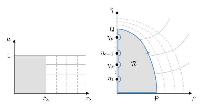
Figure 1: On the left we depict the $(r_{\Sigma},\mu)$ plane. The relevant region is the strip $r_{\Sigma}\geq 0$, $0\leq\mu\leq 1$. The shaded area corresponds to the portion $D\times S^{5}$ that is excised to make room for the puncture. The value $\bar{r}_{\Sigma}$ is the radius of the disk $D$. We also include lines of constant $r_{\Sigma}$ and lines of constant $\mu$. On the right we depict the $(\rho,\eta)$ plane. The region $\mathcal{R}$ corresponds to the relevant portion of the puncture geometry $X_{7}$. The portion of the $(\rho,\eta)$ plane outside the region $\mathcal{R}$ corresponds to the bulk of the Riemann surface. We depict the qualitative behavior of lines of constant $r_{\Sigma}$ and $\mu$ as they appear in $(\rho,\eta)$ coordinates.

In performing the gluing of puncture geometry and bulk geometry, the angular coordinate $\chi$ in the puncture geometry is given in terms of bulk coordinates by

$$\chi=\phi+\beta\ .$$ (E.23)

In particular, this relation implies that the angle $\chi$ is gauged by the external connection for the angle $\phi$,

$$D\chi=d\chi-A^{\phi}\ ,\qquad F^{\phi}=dA^{\phi}\ ,$$ (E.24)

where $A^{\phi}$, $F^{\phi}$ are the same as in (E.6). As soon as the external connection $A^{\phi}$ is activated, the 1-form $D\beta$ in (E.18) has to be improved to

$$\widetilde{D\beta}=d\beta-L\,D\chi\ .$$ (E.25)

For later applications, we also need to point out that the internal part of the $\phi$ connection on the disk $D$ on the Riemann surface is conveniently parametrized as

$$D\phi=d\phi-A^{\phi}-\mathcal{A}_{\Sigma}\ ,\qquad\mathcal{A}_{\Sigma}=U(r_{\Sigma})\,d\beta\ ,$$ (E.26)

where the function $U$ vanishes at $r_{\Sigma}=0$ in order to ensure regularity of $A_{\Sigma}$. Since $U$ is a function of $r_{\Sigma}$ only, it is constant on the locus $r_{\Sigma}=\bar{r}_{\Sigma}$. Let us therefore write $\overline{U}=U(\bar{r}_{\Sigma})$. Recall that the gluing is implicitly performed in the limit of small disk, $\bar{r}_{\Sigma}\rightarrow 0$. In this limit, we have $\overline{U}\rightarrow 0$.

The form $E_{5}$ for the puncture geometry

Our next task is to write down the most general $E_{5}$ compatible with the topology and isometries of the puncture geometry, and impose that each term in $dE_{5}$ has at most two internal legs. The most general allowed $E_{5}$ is found to be

$$E_{5} =\bigg{[}d\bigg{(}Y\,\frac{D\chi}{2\pi}-W\,\frac{\widetilde{D\beta}}{2\pi}\bigg{)}+\Lambda\,d\rho\,d\eta\bigg{]}\,e_{3}^{SO(4)}$$

$$+\bigg{[}\sigma_{1}\,\frac{D\chi}{2\pi}+\sigma_{2}\,\frac{\widetilde{D\beta}}{2\pi}+\lambda_{1}\bigg{]}\,\frac{\epsilon_{abcd}\,F^{ab}\,F^{cd}}{(2\pi)^{2}}$$

$$+\bigg{[}\sigma_{3}\,\frac{D\chi}{2\pi}+\sigma_{4}\,\frac{\widetilde{D\beta}}{2\pi}+\lambda_{2}\bigg{]}\,\frac{\epsilon_{abcd}\,F^{ab}\,Dy^{c}\,Dy^{d}}{(2\pi)^{2}}$$

$$+\bigg{[}\sigma_{0}\,\frac{F^{\phi}}{2\pi}-d\bigg{(}\sigma_{3}\,\frac{D\chi}{2\pi}\bigg{)}-d\bigg{(}\sigma_{4}\,\frac{\widetilde{D\beta}}{2\pi}\bigg{)}-d\lambda_{2}\Big{]}\,\frac{\epsilon_{abcd}\,F^{ab}\,y^{c}\,Dy^{d}}{(2\pi)^{2}}\ .$$ (E.27)

In the above expression, the 3-form $e_{3}^{SO(4)}$ is the global angular form of $SO(4)$,

$$e_{3}^{SO(4)}=\frac{1}{2\pi^{2}}\,\bigg{[}\frac{1}{3!}\,\epsilon_{abcd}\,y^{a}\,Dy^{b}\,Dy^{c}\,Dy^{d}-\frac{1}{4}\,\epsilon_{abcd}\,F^{ab}\,y^{c}\,Dy^{d}\bigg{]}\ .$$ (E.28)

It satisfies

$$\int_{S^{3}_{\Omega}}e_{3}^{SO(4)}=1\ ,\qquad de_{3}^{SO(4)}=-\frac{1}{8}\,\frac{\epsilon_{abcd}\,F^{ab}\,F^{cd}}{(2\pi)^{2}}=-\chi_{4}(SO(4))\ .$$ (E.29)

The quantities $Y$, $W$, $\sigma_{0,1,2,3}$, $\Lambda$ are functions of $\rho$, $\eta$, while $\lambda_{1,2}$ are 1-forms in the $(\rho,\eta)$ plane. These objects are not uniquely determined, but are constrained by regularity of $E_{5}$ and flux quantization.

Let us first focus on the functions $Y$, $W$. They enter $E_{5}$ via the closed 2-form

$$\mathcal{E}_{2}=d\bigg{[}Y\,\frac{D\chi}{2\pi}-W\,\frac{\widetilde{D\beta}}{2\pi}\bigg{]}=(dY+W\,dL)\,\frac{D\chi}{2\pi}-dW\,\frac{\widetilde{D\beta}}{2\pi}-(Y+W\,L)\,\frac{F^{\phi}}{2\pi}\ .$$ (E.30)

This 2-form is exactly the same as the one that appears in the M-theory setup of Bah:2018jrv ; Bah:2019jts . This means that we can repeat the flux quantization analysis of Bah:2018jrv ; Bah:2019jts almost verbatim, keeping in mind that the role of $S^{2}_{\Omega}$ in M-theory is now played by $S^{3}_{\Omega}$. It follows that the conditions on $Y$, $W$ that were derived in Bah:2018jrv ; Bah:2019jts are also true in the present context. They can be summarized as follows:

• The function $W=W(\rho,\eta)$ is smooth for $\rho\geq 0$, $\eta\geq 0$, and vanishes for $\eta=0$ for any $\rho$,

  $$W(\rho,0)=0\ .$$ (E.31)

  The values of $W$ at the locations of the monopoles along the $\eta$ axis at $\rho=0$ satisfy

  $$W(0,\eta_{a})=w_{a}\ ,$$ (E.32)

  where $\{w_{a}\}_{a=1}^{p}$ is an increasing sequence of positive integers.

• The function $Y=Y(\rho,\eta)$ is smooth away from the $\eta$ axis at $\rho=0$, and vanishes at $\eta=0$ for any $\rho$,

  $$Y(\rho,0)=0\ .$$ (E.33)

  Moreover, $Y$ is piecewise constant (hence discontinuous) along the $\eta$ axis,

  $$Y(0,\eta) =y_{a}\phantom{{}:=N}\qquad\text{for $\eta_{a}<\eta<\eta_{a+1}$}\ ,\qquad a=1,\dots,p-1\ ,$$

  $$Y(0,\eta) =y_{p}:=N\qquad\text{for $\eta>\eta_{p}$}\ .$$ (E.34)

  The quantities $y_{a}$ are all positive integers.

• Even though $L$ and $Y$ are both discontinuous along the $\eta$ axis at $\rho=0$, the form $\mathcal{E}_{2}$ is free from discontinuities, thanks to the “sum rule”

  $$y_{a}=\sum_{b=1}^{a}w_{b}\,k_{b}\ .$$ (E.35)

  In particular, selecting $a=p$ and using $y_{p}=N$, we get the relation

  $$N=\sum_{a=1}^{p}w_{a}k_{a}\ ,$$ (E.36)

  which defines a partition of $N$.

In direct analogy with the M-theory analysis, we observe that regularity and flux quantization of $E_{5}$ imply that the class of punctures we are studying are labelled by partitions of $N$. It would be interesting to have a purely field-theoretic understanding of this feature of punctures in 4d $\mathcal{N}=4$ SYM theory.

When the puncture geometry is glued to the bulk geometry, the functions $Y$, $W$ are related to the function $\gamma$ in (E.3) and $U$ in (E.26). The analysis of Bah:2019jts shows that the gluing condition is

$$Y+W\,L=N\,\gamma\ ,\qquad W=N\,\gamma\,(1+\overline{U})\qquad\text{along the $\mathsf{PQ}$ arc}\ .$$ (E.37)

We have recalled that the $\mathsf{PQ}$ arc sits at $r_{\Sigma}=\bar{r}_{\Sigma}$, hence $U=\overline{U}$ constant along the $\mathsf{PQ}$ arc.

Finally, let us collect some conditions on the functions $\sigma_{1,2,3,4}$ that stem from regularity of $E_{5}$ and smooth gluing onto the bulk geometry. The $\chi$ circle in $\mathbb{R}^{3}$ shrinks along the $\eta$ axis. This implies the regularity conditions

$$\sigma_{1}\Big{|}_{\rho=0}=\sigma_{3}\Big{|}_{\rho=0}=0\ .$$ (E.38)

We also know that the circle $S^{1}_{\beta}$ shrinks at the location of the monopoles. This gives the regularity conditions

$$\sigma_{2}(0,\eta_{a})=\sigma_{4}(0,\eta_{a})=0\ ,\qquad a=1,\dots,p\ .$$ (E.39)

Next, let us compare the terms with $\epsilon_{abcd}\,F^{ab}\,F^{cd}$ in the expressions (E.3) and (E) for $E_{5}$ in the bulk and for a puncture. In (E.3) the prefactor of $\epsilon_{abcd}\,F^{ab}\,F^{cd}$ has only legs along $D\phi$, while in (E) it is a combination of $D\chi$ and $\widetilde{D\beta}$. These different prefactors must agree along the $\mathsf{PQ}$ arc. In particular, on this arc there should be no $d\beta$ term in the prefactor of $\epsilon_{abcd}\,F^{ab}\,F^{cd}$ in (E). This implies

$$\sigma_{1}+\sigma_{2}-L\,\sigma_{2}=0\qquad\text{along the $\mathsf{PQ}$ arc}\ .$$ (E.40)

In a similar way, matching terms with $\epsilon_{abcd}\,F^{ab}\,Dy^{d}\,Dy^{d}$ in (E.3) and (E) leads to the condition

$$\sigma_{3}+\sigma_{4}-L\,\sigma_{4}=0\qquad\text{along the $\mathsf{PQ}$ arc}\ .$$ (E.41)

Let us point out that, by arguments similar to those of the previous paragraphs, one can also argue that $\lambda_{1,2}$ and $\Lambda$ should be zero in order to ensure a smooth gluing between puncture and bulk $E_{5}$ forms. We will not make direct use of this observation, however, because the anomaly inflow result turns out to be automatically independent of $\lambda_{1,2}$, $\Lambda$.

E.6 The integral of $E_{5}\,dE_{5}$ in the puncture geometry

We may use again (E.14) for the integration over $S^{3}_{\Omega}$. Both the $\chi$ and the $\beta$ circles have periodicity $2\pi$. The orientation convention that fits with the orientation of the bulk is the one that assigns a positive orientation to $d\rho\,d\eta\,d\chi\,d\beta\,{\rm vol}_{S^{3}_{\Omega}}$. One finds

$$\int_{X_{7}}E_{5}\,dE_{5}=\frac{\epsilon_{abcd}\,F^{ab}\,F^{cd}}{(2\pi)^{2}}\,\int_{\mathcal{R}_{2}}\,\mathcal{S}_{2}\ ,$$ (E.42)

where $\mathcal{R}_{2}$ is the region in the $(\rho,\eta)$ plane depicted in figure 1, and $\mathcal{S}_{2}$ is the following 2-form in the $(\rho,\eta)$ plane,

$$\mathcal{S}_{2} =-\frac{1}{4}\,d(Y+W\,L)\,dW$$

$$-\bigg{[}dW\,d(\sigma_{1}+\sigma_{2}-L\,\sigma_{2})+d(Y+W\,L)\,d\sigma_{2}-dW\,d\sigma_{2}\bigg{]}$$

$$+\frac{1}{4}\,\bigg{[}dW\,d(\sigma_{3}+\sigma_{4}-L\,\sigma_{4})+d(Y+W\,L)\,d\sigma_{4}-dW\,d\sigma_{4}\bigg{]}\ .$$ (E.43)

As we can see, the result seems to depend on the unspecified functions $\sigma_{1,2,3,4}$. We now demonstrate, however, that all dependence on $\sigma_{1,2,3,4}$ drops away after integrating on the region $\mathcal{R}_{2}$. To this end, it is convenient to write

$$\mathcal{S}_{2}=d\mathcal{S}_{1}\ ,\qquad\mathcal{S}_{1} =\frac{1}{4}\,W\,d(Y+W\,L)$$

$$-\bigg{[}W\,d(\sigma_{1}+\sigma_{2}-L\,\sigma_{2})+(Y+W\,L)\,d\sigma_{2}-W\,d\sigma_{2}\bigg{]}$$

$$+\frac{1}{4}\,\bigg{[}W\,d(\sigma_{3}+\sigma_{4}-L\,\sigma_{4})+(Y+W\,L)\,d\sigma_{4}-W\,d\sigma_{4}\bigg{]}\ .$$ (E.44)

By Stokes’ theorem,

$$\int_{\mathcal{R}_{2}}\mathcal{S}_{2}=\int_{\partial\mathcal{R}_{2}}\mathcal{S}_{1}\ .$$ (E.45)

The boundary $\partial\mathcal{R}_{2}$ consists of a horizontal segment along the $\rho$ axis, the $\mathsf{PQ}$ arc, and a collection of intervals along the $\eta$ axis, connected by small semicircles around the monopole sources, as shown in figure 1. We discuss these boundary components in turn.

The horizontal segment along the $\rho$ axis.

We know that $W$ and $Y$ vanish along the $\rho$ axis at $\eta=0$. It follows that $\mathcal{S}_{1}$ is zero along the horizontal segment of $\partial\mathcal{R}_{2}$.

The $\mathsf{PQ}$ arc.

The integral of the term $\frac{1}{4}\,W\,d(Y+W\,L)$ in $\mathcal{S}_{1}$ along the $\mathsf{PQ}$ arc is non-zero. As in appendix B of Bah:2019jts , this term is interpreted as a bulk contribution, rather than as a puncture contribution. Next, we argue that all terms in $\mathcal{S}_{1}$ with $\sigma_{1,2,3,4}$ integrate to zero along the $\mathsf{PQ}$ arc. To see this, we use (E.40) and (E.37) to write

$$W\,d(\sigma_{1}+\sigma_{2}-L\,\sigma_{2})+(Y+W\,L)\,d\sigma_{2}-W\,d\sigma_{2}=$$

$$=-N\,\overline{U}\,\gamma\,d\sigma_{2}\qquad\text{along the $\mathsf{PQ}$ arc}\ .$$ (E.46)

The gluing is performed in the limit of small disk radius, which implies $\overline{U}\rightarrow 0$. As a result, the terms in $\mathcal{S}_{1}$ with $\sigma_{1,2}$ do not yield any contribution from integration along the $\mathsf{PQ}$ arc. The terms with $\sigma_{3,4}$ are treated in a completely analogous way, making use of (E.41).

The intervals along the $\eta$ axis.

We consider each interval $(\eta_{a-1},\eta_{a})$, $a=1,\dots,p$, together with the interval that connects the last monopole at $\eta=\eta_{p}$ with the point $\mathsf{Q}$, which we denote schematically as $(\eta_{p},\mathsf{Q})$. First of all, we compute

$$\int_{(\eta_{a-1},\eta_{a})}\frac{1}{4}\,W\,d(Y+W\,L)=\int_{(\eta_{a-1},\eta_{a})}d\bigg{[}\frac{1}{8}\,\ell_{a}\,W^{2}\bigg{]}=\frac{1}{8}\,\ell_{a}\,(w_{a}^{2}-w_{a-1}^{2})\ ,$$ (E.47)

where we used the fact that $Y=y_{a-1}$ constant and $L=\ell_{a}$ constant in the interval $(\eta_{a-1},\eta_{a})$. If we consider the last interval $(\eta_{p},\mathsf{Q})$, we have $L=0$ and therefore we get no contribution.

Next, we argue that the terms with $\sigma_{1,2,3,4}$ in $\mathcal{S}_{1}$ drop away from all integrals over $(\eta_{a-1},\eta_{a})$ and $(\eta_{p},\mathsf{Q})$. If we consider the interval $(\eta_{a-1},\eta_{a})$, we can use $L=\ell_{a}$, $Y=y_{a-1}$, and the regularity condition (E.38) on $\sigma_{1}$ to observe that

$$W\,d(\sigma_{1}+\sigma_{2}-L\,\sigma_{2})+(Y+W\,L)\,d\sigma_{2}-W\,d\sigma_{2}=$$ (E.48)

$$=y_{a-1}\,d\sigma_{2}\qquad\text{along the interval $(\eta_{a-1},\eta_{a})$}\ .$$

When this 1-form is integrated on $(\eta_{a-1},\eta_{a})$, the result is proportional to the difference $\sigma_{2}(0,\eta_{a})-\sigma_{2}(0,\eta_{a-1})$, which is zero thanks to the regularity condition (E.39). In a similar way, if we consider the last interval $(\eta_{p},\mathsf{Q})$, we can use $L=0$, $Y=N$, and get

$$W\,d(\sigma_{1}+\sigma_{2}-L\,\sigma_{2})+(Y+W\,L)\,d\sigma_{2}-W\,d\sigma_{2}=$$ (E.49)

$$=N\,d\sigma_{2}\qquad\text{along the interval $(\eta_{p},\mathsf{Q})$}\ .$$

To show that this integrates to zero we must argue that $\sigma_{2}$ vanishes at point $\mathsf{Q}$. This is indeed the case, because $\mathsf{Q}$ lies at the intersection of the $\eta$ axis with the $\mathsf{PQ}$ arc, and therefore we can combine (E.38) and (E.40) and infer that $\sigma_{2}$ is zero at $\mathsf{Q}$.

The fact that all terms in $\mathcal{S}_{1}$ with $\sigma_{1,3}$ do not contribute to integrals over $(\eta_{a-1},\eta_{a})$ and $(\eta_{p},\mathsf{Q})$ is shown in a completely analogous way.

Small semicircles around the monopole sources.

The small semicircles do not give any non-zero contribution in the limit in which their radius goes to zero. To see this, let us introduce coordinates $(R_{a},\tau_{a})$ in the vicinity of the $a$-th monopole, as

$$\eta=\eta_{a}+R_{a}\,\tau_{a}\ ,\qquad\rho=R_{a}\,\sqrt{1-\tau_{1}^{a}}\ ,$$ (E.50)

with the range of $\tau_{a}$ being $[-1,1]$. The small semicircle is described by $R_{a}=\text{const}\rightarrow 0$. To argue that the term $W\,d(Y+W\,L)$ in $\mathcal{S}_{1}$ does not contribute when integrated on the small semicircle around the $a$-th monopole, we recall that both $W$ and the combination $Y+W\,L$ are continuous along the $\eta$ axis (while $Y$ and $L$ separately are piecewise constant). As a result, for small constant $R_{a}$, we have

$$\int_{\text{semicircle}}W\,d(Y+W\,L)\approx w_{a}\,\int_{-1}^{1}d\tau_{a}\,\partial_{\tau_{a}}(Y+W\,L)=w_{a}\,\Big{[}Y+W\,L\Big{]}_{\eta=\eta_{a}-R_{a}}^{\eta=\eta_{a}+R_{a}}\rightarrow 0\ .$$ (E.51)

In the first step we used the fact that, to leading order as $R_{a}\rightarrow 0$, $W$ is approximated by its value $w_{a}$ at $(\rho,\eta)=(0,\eta_{a})$ because it is continuous near that point. In the last step we get zero because $Y+W\,L$ tends to the same value as we approach $\eta_{a}$ from below or above. All other terms in $\mathcal{S}_{1}$ are treated in a similar way. We need to recall that $\sigma_{1}$ and $\sigma_{3}$ vanish along the $\eta$ axis, and that $\sigma_{2}$ and $\sigma_{4}$ vanish at the location of the monopoles.

Summary.

There is only one non-zero contribution to the puncture anomaly, given by summing terms of the form (E.47). Notice that the boundary $\partial\mathcal{R}_{2}$ must be traversed in counterclockwise orientation, which means that each interval on the $\eta$ axis is considered with a negative orientation. As a result, we arrive at

$$\int_{X_{7}}E_{5}\,dE_{5}=-\frac{1}{8}\,\frac{\epsilon_{abcd}\,F^{ab}\,F^{cd}}{(2\pi)^{2}}\,\sum_{a=1}^{p}\ell_{a}\,(w_{a}^{2}-w_{a-1}^{2})\ .$$ (E.52)

References

- (1) D. Gaiotto, “N=2 dualities,” JHEP 08 (2012) 034, arXiv:0904.2715 [hep-th].
- (2) D. Gaiotto, G. W. Moore, and A. Neitzke, “Wall-crossing, Hitchin Systems, and the WKB Approximation,” arXiv:0907.3987 [hep-th].
- (3) K. Maruyoshi, M. Taki, S. Terashima, and F. Yagi, “New Seiberg Dualities from N=2 Dualities,” JHEP 09 (2009) 086, arXiv:0907.2625 [hep-th].
- (4) F. Benini, Y. Tachikawa, and B. Wecht, “Sicilian gauge theories and N=1 dualities,” JHEP 01 (2010) 088, arXiv:0909.1327 [hep-th].
- (5) I. Bah and B. Wecht, “New N=1 Superconformal Field Theories In Four Dimensions,” JHEP 07 (2013) 107, arXiv:1111.3402 [hep-th].
- (6) I. Bah, C. Beem, N. Bobev, and B. Wecht, “AdS/CFT Dual Pairs from M5-Branes on Riemann Surfaces,” Phys. Rev. D85 (2012) 121901, arXiv:1112.5487 [hep-th].
- (7) I. Bah, C. Beem, N. Bobev, and B. Wecht, “Four-Dimensional SCFTs from M5-Branes,” JHEP 06 (2012) 005, arXiv:1203.0303 [hep-th].
- (8) I. Bah and E. Nardoni, “Structure of Anomalies of 4d SCFTs from M5-branes, and Anomaly Inflow,” JHEP 03 (2019) 024, arXiv:1803.00136 [hep-th].
- (9) I. Bah, F. Bonetti, R. Minasian, and E. Nardoni, “Class Anomalies from M-theory Inflow,” Phys. Rev. D99 no. 8, (2019) 086020, arXiv:1812.04016 [hep-th].
- (10) I. Bah, F. Bonetti, R. Minasian, and E. Nardoni, “Anomaly Inflow for M5-branes on Punctured Riemann Surfaces,” JHEP 06 (2019) 123, arXiv:1904.07250 [hep-th].
- (11) I. Bah, F. Bonetti, R. Minasian, and E. Nardoni, “Anomalies of QFTs from M-theory and Holography,” arXiv:1910.04166 [hep-th].
- (12) I. Bah and F. Bonetti, “Anomaly Inflow, Accidental Symmetry, and Spontaneous Symmetry Breaking,” arXiv:1910.07549 [hep-th].
- (13) M. J. Duff, J. T. Liu, and R. Minasian, “Eleven-dimensional origin of string-string duality: A One loop test,” Nucl. Phys. B452 (1995) 261–282, arXiv:hep-th/9506126 [hep-th].
- (14) E. Witten, “Five-brane effective action in M theory,” J. Geom. Phys. 22 (1997) 103–133, arXiv:hep-th/9610234 [hep-th].
- (15) D. Freed, J. A. Harvey, R. Minasian, and G. W. Moore, “Gravitational anomaly cancellation for M theory five-branes,” Adv. Theor. Math. Phys. 2 (1998) 601–618, arXiv:hep-th/9803205 [hep-th].
- (16) J. A. Harvey, R. Minasian, and G. W. Moore, “NonAbelian tensor multiplet anomalies,” JHEP 09 (1998) 004, arXiv:hep-th/9808060 [hep-th].
- (17) C. Lawrie, D. Martelli, and S. Schäfer-Nameki, “Theories of Class F and Anomalies,” JHEP 10 (2018) 090, arXiv:1806.06066 [hep-th].
- (18) M. Fazzi and A. Tomasiello, “Holography, Matrix Factorizations and K-stability,” arXiv:1906.08272 [hep-th].
- (19) H. Kim and P. Yi, “D-brane anomaly inflow revisited,” JHEP 02 (2012) 012, arXiv:1201.0762 [hep-th].
- (20) S. Goldberg, Curvature and Homology. ISSN. Elsevier Science, 2011. https://books.google.com/books?id=aD0_kF3L0qMC.
- (21) S. Benvenuti, L. A. Pando Zayas, and Y. Tachikawa, “Triangle anomalies from Einstein manifolds,” Adv. Theor. Math. Phys. 10 no. 3, (2006) 395–432, arXiv:hep-th/0601054 [hep-th].
- (22) S. Franco, A. Hanany, D. Martelli, J. Sparks, D. Vegh, and B. Wecht, “Gauge theories from toric geometry and brane tilings,” JHEP 01 (2006) 128, arXiv:hep-th/0505211 [hep-th].
- (23) S. Benvenuti and A. Hanany, “New results on superconformal quivers,” JHEP 04 (2006) 032, arXiv:hep-th/0411262 [hep-th].
- (24) I. R. Klebanov and E. Witten, “Superconformal field theory on three-branes at a Calabi-Yau singularity,” Nucl. Phys. B536 (1998) 199–218, arXiv:hep-th/9807080 [hep-th].
- (25) M. R. Douglas and G. W. Moore, “D-branes, quivers, and ALE instantons,” arXiv:hep-th/9603167 [hep-th].
- (26) C. V. Johnson and R. C. Myers, “Aspects of type IIB theory on ALE spaces,” Phys. Rev. D55 (1997) 6382–6393, arXiv:hep-th/9610140 [hep-th].
- (27) C. Vafa and E. Witten, “A Strong coupling test of S duality,” Nucl. Phys. B431 (1994) 3–77, arXiv:hep-th/9408074 [hep-th].
- (28) M. Bershadsky, A. Johansen, V. Sadov, and C. Vafa, “Topological reduction of 4-d SYM to 2-d sigma models,” Nucl. Phys. B448 (1995) 166–186, arXiv:hep-th/9501096 [hep-th].
- (29) J. M. Maldacena and C. Nunez, “Supergravity description of field theories on curved manifolds and a no go theorem,” Int. J. Mod. Phys. A16 (2001) 822–855, arXiv:hep-th/0007018 [hep-th]. [,182(2000)].
- (30) F. Benini and N. Bobev, “Exact two-dimensional superconformal R-symmetry and c-extremization,” Phys. Rev. Lett. 110 no. 6, (2013) 061601, arXiv:1211.4030 [hep-th].
- (31) F. Benini and N. Bobev, “Two-dimensional SCFTs from wrapped branes and c-extremization,” JHEP 06 (2013) 005, arXiv:1302.4451 [hep-th].
- (32) N. Bobev, K. Pilch, and O. Vasilakis, “(0, 2) SCFTs from the Leigh-Strassler fixed point,” JHEP 06 (2014) 094, arXiv:1403.7131 [hep-th].
- (33) F. Benini, N. Bobev, and P. M. Crichigno, “Two-dimensional SCFTs from D3-branes,” JHEP 07 (2016) 020, arXiv:1511.09462 [hep-th].
- (34) N. Bobev and P. M. Crichigno, “Universal RG Flows Across Dimensions and Holography,” JHEP 12 (2017) 065, arXiv:1708.05052 [hep-th].
- (35) K. A. Intriligator and B. Wecht, “The Exact superconformal R symmetry maximizes a,” Nucl. Phys. B667 (2003) 183–200, arXiv:hep-th/0304128 [hep-th].
- (36) D. Gaiotto and J. Maldacena, “The Gravity duals of N=2 superconformal field theories,” JHEP 10 (2012) 189, arXiv:0904.4466 [hep-th].
- (37) F. Denef, “Les Houches Lectures on Constructing String Vacua,” Les Houches 87 (2008) 483–610, arXiv:0803.1194 [hep-th].
- (38) T. Weigand, “F-theory,” PoS TASI2017 (2018) 016, arXiv:1806.01854 [hep-th].
- (39) K. Dasgupta, G. Rajesh, and S. Sethi, “M theory, orientifolds and G - flux,” JHEP 08 (1999) 023, arXiv:hep-th/9908088 [hep-th].
- (40) T. W. Grimm and H. Hayashi, “F-theory fluxes, Chirality and Chern-Simons theories,” JHEP 03 (2012) 027, arXiv:1111.1232 [hep-th].
- (41) M. Cvetic, T. W. Grimm, and D. Klevers, “Anomaly Cancellation And Abelian Gauge Symmetries In F-theory,” JHEP 02 (2013) 101, arXiv:1210.6034 [hep-th].
- (42) K. Pilch and N. P. Warner, “A New supersymmetric compactification of chiral IIB supergravity,” Phys.Lett.B 487 (2000) 22–29, arXiv:hep-th/0002192.
- (43) J. P. Gauntlett, D. Martelli, J. Sparks, and D. Waldram, “Supersymmetric AdS(5) solutions of type IIB supergravity,” Class.Quant.Grav. 23 (2006) 4693–4718, arXiv:hep-th/0510125.
- (44) C. Couzens, “Supersymmetric AdS solutions of type IIB supergravity without D3 branes,” JHEP 01 (2017) 041, arXiv:1609.05039 [hep-th].
- (45) N. Bobev, P. Bomans, and F. F. Gautason, “Wrapped Branes and Punctured Horizons,” arXiv:1912.04779 [hep-th].
- (46) F. Apruzzi, F. Hassler, J. J. Heckman, and I. V. Melnikov, “UV Completions for Non-Critical Strings,” JHEP 07 (2016) 045, arXiv:1602.04221 [hep-th].
- (47) F. Apruzzi, F. Hassler, J. J. Heckman, and I. V. Melnikov, “From 6D SCFTs to Dynamic GLSMs,” Phys. Rev. D96 no. 6, (2017) 066015, arXiv:1610.00718 [hep-th].
- (48) C. Lawrie, S. Schafer-Nameki, and T. Weigand, “Chiral 2d theories from N = 4 SYM with varying coupling,” JHEP 04 (2017) 111, arXiv:1612.05640 [hep-th].
- (49) C. Couzens, C. Lawrie, D. Martelli, S. Schafer-Nameki, and J.-M. Wong, “F-theory and /,” JHEP 08 (2017) 043, arXiv:1705.04679 [hep-th].
- (50) C. Couzens, D. Martelli, and S. Schafer-Nameki, “F-theory and / ,” JHEP 06 (2018) 008, arXiv:1712.07631 [hep-th].
- (51) J. J. Heckman and T. Rudelius, “Top Down Approach to 6D SCFTs,” J.Phys.A 52 no. 9, (2019) 093001, arXiv:1805.06467 [hep-th].
- (52) I. Antoniadis, S. Ferrara, R. Minasian, and K. S. Narain, “R**4 couplings in M and type II theories on Calabi-Yau spaces,” Nucl. Phys. B507 (1997) 571–588, arXiv:hep-th/9707013 [hep-th].
- (53) J. T. Liu and R. Minasian, “Computing 1/ corrections in AdS/CFT,” arXiv:1010.6074 [hep-th].
- (54) M. Nakahara, Geometry, topology and physics. 2003.
- (55) M. Bianchi, A. Collinucci, and L. Martucci, “Magnetized E3-brane instantons in F-theory,” JHEP 12 (2011) 045, arXiv:1107.3732 [hep-th].
- (56) T. Pantev and E. Sharpe, “Duality group actions on fermions,” JHEP 11 (2016) 171, arXiv:1609.00011 [hep-th].
- (57) R. Minasian, S. Sasmal, and R. Savelli, “Discrete anomalies in supergravity and consistency of string backgrounds,” JHEP 02 (2017) 025, arXiv:1611.09575 [hep-th].