The solar wind from a stellar perspective:

Abstract

Context. Due to the effects that they can have on the atmospheres of exoplanets, stellar winds have recently received significant attention in the literature. Alfvén-wave-driven 3D magnetohydrodynamic (MHD) models, which are increasingly used to predict stellar wind properties, contain unconstrained parameters and rely on low-resolution stellar magnetograms.

Aims. In this paper, we explore the effects of the input Alfvén wave energy flux and the surface magnetogram on the wind properties predicted by the Alfvén Wave Solar Model (AWSoM) model for both the solar and stellar winds.

Methods. We lowered the resolution of two solar magnetograms during solar cycle maximum and minimum using spherical harmonic decomposition. The Alfvén wave energy was altered based on non-thermal velocities determined from a far ultraviolet (FUV) spectrum of the solar twin 18 Sco. Additionally, low-resolution magnetograms of three solar analogues, 18 Sco, HD 76151, and HN Peg, were obtained using Zeeman Doppler imaging (ZDI) and used as a proxy for the solar magnetogram. Finally, the simulated wind properties were compared to Advanced Composition Explorer (ACE) observations.

Results. AWSoM simulations using well constrained input parameters taken from solar observations can reproduce the observed solar wind mass loss and angular momentum loss rates. The simulated wind velocity, proton density, and ram pressure differ from ACE observations by a factor of approximately two. The resolution of the magnetogram has a small impact on the wind properties and only during cycle maximum. However, variation in Alfvén wave energy influences the wind properties irrespective of the solar cycle activity level. Furthermore, solar wind simulations carried out using the low-resolution magnetogram of the three stars instead of the solar magnetogram could lead to an order of a magnitude difference in the simulated solar wind properties.

Conclusions. The choice in Alfvén energy has a stronger influence on the wind output compared to the magnetogram resolution. The influence could be even stronger for stars whose input boundary conditions are not as well constrained as those of the Sun. Unsurprisingly, replacing the solar magnetogram with a stellar magnetogram could lead to completely inaccurate solar wind properties, and should be avoided in solar and stellar wind simulations. Further observational and theoretical work is needed to fully understand the complexity of solar and stellar winds.

1 Introduction

Stellar magnetic fields are responsible for a large number of phenomena, including the emission of high-energy radiation and the formation of supersonic ionised winds. By driving atmospheric processes such as non-thermal losses to space, these winds play an important role in the evolution of planetary atmospheres and habitability (Tian et al., 2008; Kislyakova et al., 2014b; Airapetian et al., 2017). As an example, the strong solar wind of the young Sun (Johnstone et al., 2015a; Airapetian & Usmanov, 2016) in combination with the weaker magnetic field of early Earth (Tarduno et al., 2010) led to higher compression of the Earth’s magnetosphere. This resulted in wider opening of polar ovals and higher atmospheric escape rates than at present (Airapetian et al., 2016). It has been shown that planetary atmospheric loss in planets with a magnetosphere depends on the interplay between the solar wind strength, wind capture area of the planetary magnetosphere, and the ability of the magnetosphere to recapture the atmospheric outflow, although the effect of magnetospheric compression on atmospheric loss rates are currently up for debate (Blackman & Tarduno, 2018). For planets lacking any intrinsic magnetic field, the incoming stellar wind interacts directly with the atmosphere, leading to atmospheric escape through the plasma wake and from a boundary layer of the induced magnetosphere (Barabash et al., 2007; Lundin, 2011). Venus-like CO₂-rich atmospheres are less prone to expansion and escape, but they are still sensitive to enhanced X-ray and extreme ultraviolet (XUV) fluxes, and wind erosion (Lichtenegger et al., 2010; Johnstone et al., 2018). The same can be true for exoplanets orbiting young stars with stronger stellar winds leading to efficient escape of the atmosphere to space (Wood et al., 2002; Lundin, 2011). It is therefore important to investigate stellar wind properties in Sun-like stars to understand their impact on habitability and also provide constraints on planetary atmospheres.

Observations of the solar wind taken by satellites such as the Advanced Composition Explorer (ACE, Stone et al., 1998; McComas et al., 1998) and Ulysses (McComas et al., 2003) have greatly improved our knowledge and understanding of the solar wind properties. The solar wind can be broken down into the fast and the slow wind with median wind speeds of approximately 760 km s^-1 and 400 km s^-1 respectively (McComas et al., 2003; Johnstone et al., 2015b). The fast component arises from coronal holes and the slow component is launched from areas above closed field lines, and from the boundary regions of open and closed field lines (Krieger et al., 1973). As the magnetic geometry of the Sun changes during the solar cycle, the locations of the fast and slow components change without any considerable changes in their properties, such as speed or mass flux. In situ measurements by spacecrafts such as Ulysses and Voyager have found that the mass loss rate of the solar wind is $\sim$2$\mathrm{\times}$10^-14 $\mathrm{M_{\sun}}$ yr^-1, and that it changes by a factor of only two over the solar cycle (Cohen, 2011). Angular momentum loss rates vary by 30-40$\%$ over the solar cycle as shown by Finley et al. (2018). This shows that despite the dramatic change in the surface magnetic field of the Sun during the cycle, the changes in the solar wind properties are not drastic.

Unfortunately, direct measurements of the properties of low-mass stellar winds are not available; instead techniques to indirectly measure stellar winds must be used, including reconstructing astrospheric Ly-$\alpha$ absorption (Wood et al., 2001) and fitting rotational evolution models to observational constraints (Matt et al., 2015; Johnstone et al., 2015a). This is problematic for stellar wind modelling since we can neither constrain the model free parameters nor test our results observationally. Attempts have been made to detect radio free-free emissions due to the presence of stellar winds in Sun-like stars (Drake et al., 1993; van den Oord & Doyle, 1997; Gaidos et al., 2000; Villadsen et al., 2014; Fichtinger et al., 2017). Unfortunately there has been no detection so far but radio observations have provided important upper limits on the wind mass loss rates of a handful of Sun-like stars. X-ray emission due to charge exchange between ionised stellar winds and the neutral interstellar hydrogen have also been used to provide upper limits on the mass loss rate due to stellar winds (Wargelin & Drake, 2002). For a limited sample of close-in transiting hot Jupiters, Lyman-$\alpha$ observations have been used to estimate the properties of the wind of the host star (Kislyakova et al., 2014a; Vidotto & Bourrier, 2017). The indirect method of astrospheric Lyman-$\alpha$ measurements (Wood et al., 2001; Wood, 2004; Wood et al., 2005) is the only technique that has provided observed wind mass loss rates for some nearby Sun-like stars. Using this method Wood et al. (2005) showed that the mass loss rate has a power-law relation with magnetic activity, implying that more active stars have higher mass loss rates. Some stars do not appear to follow this trend and this method can only be applied to nearby stars that are surrounded by at least partially neutral interstellar medium. We are therefore heavily dependent on wind models to enhance our understanding of stellar wind properties.

Solar and stellar wind modelling faces multiple challenges, as we still lack a complete understanding of the heating, acceleration, and propagation of the wind. The outward acceleration of the wind takes place in large part due to thermal pressure gradients driven by the very large temperatures of coronal gas (Parker, 1958). However, measurements of the gas temperatures inside coronal holes show that the temperatures are not high enough to accelerate the wind to the speed of the fast component, and therefore another acceleration mechanism is required (Cranmer, 2009). The source of the wind heating and the nature of this additional acceleration mechanism are currently poorly understood (Cranmer & Winebarger, 2019). Alfvén waves are considered to be a likely key mechanism for solar wind heating and acceleration. Observations taken using Hinode (Kosugi et al., 2007) and the Solar Dynamics Observatory (SDO, Pesnell et al., 2012) have shown that Alfvénic waves in the solar chromosphere have much stronger amplitudes compared to their coronal counterpart (De Pontieu et al., 2007; McIntosh et al., 2011). The weakening of the waves as they reach the corona is attributed to the wave dissipation. The waves reflected by density and magnetic pressure gradients interact with the forward propagating waves resulting in wave dissipation, which in turn heats the lower corona. This provides the necessary energy to propagate and accelerate the wind so that it can escape from the gravity of the star (Matthaeus et al., 1999). It has been suggested that for very rapidly rotating stars, magneto-centrifugal forces also provide an important wind acceleration mechanism (Johnstone, 2017).

To tackle the wind heating problem, it has been common in solar and stellar wind models to assume a polytropic equation of state (Parker, 1965; van der Holst et al., 2007; Cohen et al., 2007; Johnstone et al., 2015b), which states that the pressure, $p$, is related to the density, $\rho$, by $p\propto\rho^{\alpha}$, where $\alpha$ is the polytropic index and is typically taken to be $\alpha\sim 1.1$. This leads to the wind being heated implicitly as it expands. Free parameters in these models are the density and temperature at the base of the wind and the value of $\alpha$, all of which can be constrained for the solar wind from in situ measurements (Johnstone et al., 2015b). However, these parameters are unconstrained for the winds of other stars. An alternative is to use solar and stellar wind models that incorporate Alfvén waves, which are becoming increasingly popular (Cranmer & Saar, 2011; Suzuki et al., 2013). Some of the earliest Alfvén-wave-driven models date back to Belcher & Davis (1971), and Alazraki & Couturier (1971). Multiple groups have developed 1D (Suzuki & Inutsuka, 2006; Cranmer et al., 2007), 2D (Usmanov et al., 2000; Matsumoto & Suzuki, 2012), and 3D (Sokolov et al., 2013; van der Holst et al., 2014; Usmanov et al., 2018) Alfvén-wave-driven solar wind models that can successfully simulate the current solar wind mass loss rates. In this work the 3D magnetohydrodynamic (MHD) model Alfvén Wave Solar Model (AWSoM; van der Holst et al. 2014) is used, where Alfvén wave propagation and partial reflection leads to a turbulent cascade, heating and accelerating the wind. The Alfvén wave energy is introduced using an input Alfvén wave Poynting flux ratio ($S_{\mathrm{A}}/B$, where $B$ is the magnetic field strength at the inner boundary of the simulation). For the Sun, Sokolov et al. (2013) established $S_{\mathrm{A}}/B$ to be 1.1 $\times$ 10⁶ Wm^-2 T^-1. In stellar wind models, $S_{\mathrm{A}}/B$ is modified using scaling laws between the X-ray activity and magnetic field $B$ of the star (Pevtsov et al., 2003; Garraffo et al., 2016; Dong et al., 2018), which requires prior information about the former parameter. As stellar X-ray activity is known to exhibit variations, this approach will also lead to variation in $S_{\mathrm{A}}/B$ for a magnetically variable star. In the solar case, the Poynting flux is well constrained from observations and nearly constant for all solar simulations. The value of $S_{\mathrm{A}}/B$ is an important input parameter, but how a change in the Poynting flux ratio quantitatively changes the final wind output remains unknown. It is important to understand the relationship between $S_{\mathrm{A}}/B$ and the coronal and wind properties, as often the Poynting flux ratio is a difficult parameter to directly determine from stellar observations.

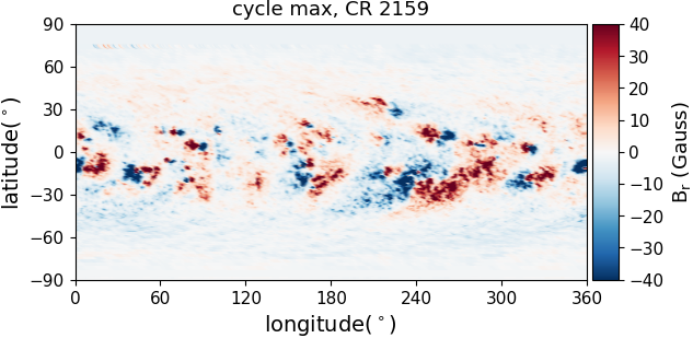
(a)

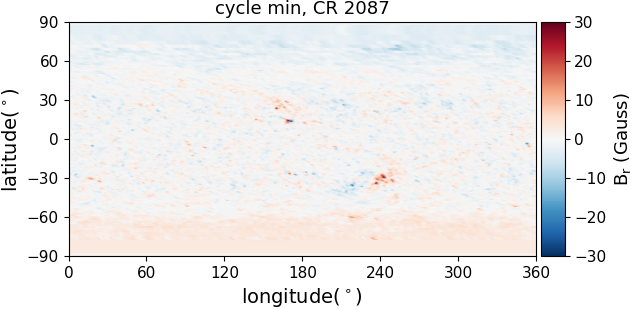
(b)

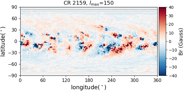
(c)

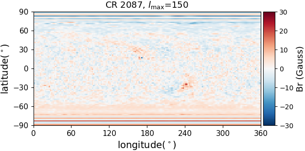
(d)

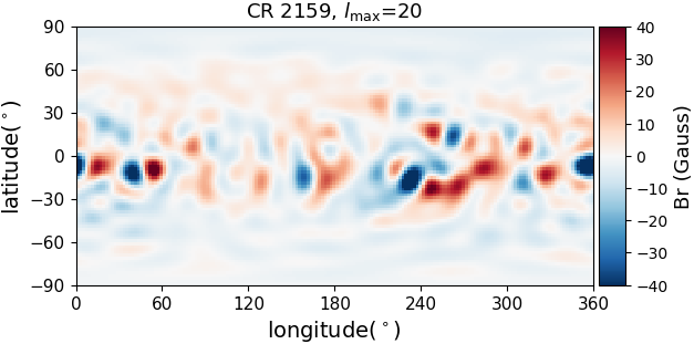
(e)

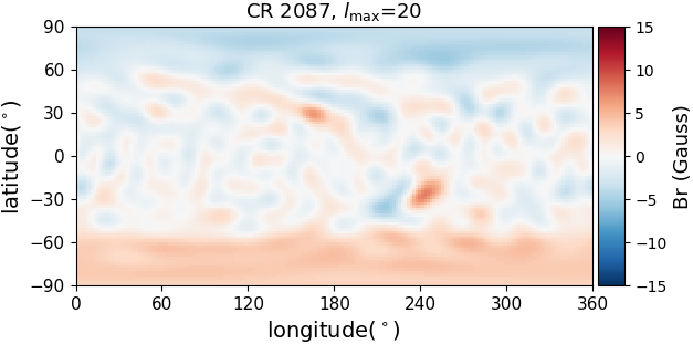
(f)

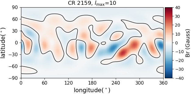
(g)

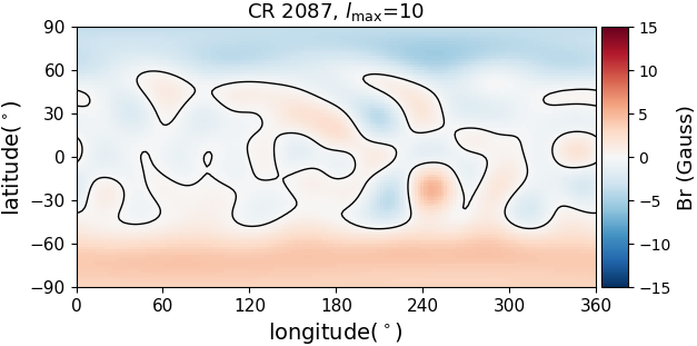
(h)

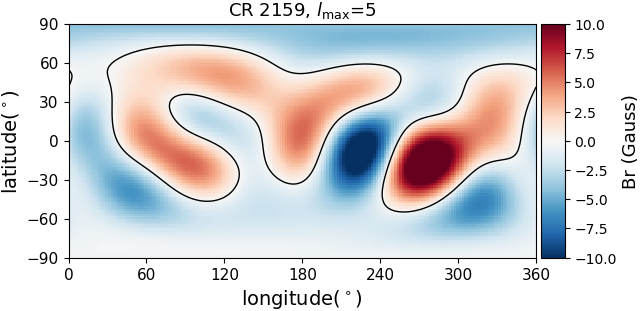
(i)

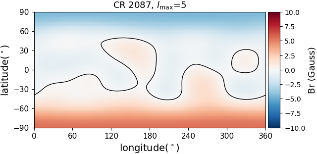
(j)

Figure 1: Synoptic GONG magnetograms during solar cycle maximum, CR 2159 (top left) and cycle minimum, CR 2087 (top right) followed by the spherical harmonic reconstructions with $l_{\mathrm{max}}$ = 150, 20, 10, and 5 respectively (second row to bottom). The magnetic maps are saturated to different values of $B_{\mathrm{r}}$, to highlight the surface magnetic features.

In 3D MHD solar wind models such as AWSoM, the input stellar surface magnetic field ensures that the model includes the correct magnetic topology of the stellar wind. In the case of the Sun, multiple solar observatories produce high-resolution synoptic magnetograms which can be used as an input (Riley et al., 2014). Stellar wind models use low-resolution magnetic maps of stars as input (Vidotto et al., 2011, 2014; Nicholson et al., 2016; Alvarado-Gómez et al., 2016a, b; Garraffo et al., 2016; Ó Fionnagáin et al., 2019), which are reconstructed using the technique of Zeeman Doppler imaging (ZDI; Semel 1989). This imagining technique reconstructs the large-scale field using spectropolarimetric observations, where the field is typically described using spherical harmonic expansion. Alternatively, solar magnetograms are sometimes used as a proxy for a given Sun-like star and are scaled to its magnetic field and activity (Dong et al., 2018). One disadvantage of using ZDI stellar magnetic maps is their resolution. A typical stellar magnetic map is reconstructed up to a spherical harmonics degree, $l_{\mathrm{max}}$, of 5-10, while a solar magnetogram can have $l_{\mathrm{max}}\geq$100. It is not known how the resolution of the magnetograms and the use of the Sun as a stellar proxy influence stellar wind properties determined from AWSoM simulations.

In this study we validate AWSoM under low-resolution input conditions, which is an important pre-requisite for the use of AWSoM in stellar cases. We investigate whether or not AWSoM solar wind simulations under low-resolution input conditions can reproduce observed ACE solar wind properties at 1 AU. Under high-resolution input conditions, AWSoM wind properties show strong agreement with observed wind properties (Oran et al., 2013; Sachdeva et al., 2019). We carry out wind simulations using low-resolution input magnetograms and a varying $S_{\mathrm{A}}/B$ ratio to investigate the sensitivity of these two input parameters in determining wind properties. Low-resolution magnetograms are obtained by performing spherical harmonic decompositions of high-resolution solar Global Oscillation Network Group (GONG) magnetograms for $l_{\mathrm{max}}$ = 150, 20, 10, and 5. We also obtain different values of $S_{\mathrm{A}}/B$ from far ultraviolet (FUV) spectral lines. The different values of $l_{\mathrm{max}}$ and $S_{\mathrm{A}}/B$ are used to create two grids of AWSoM wind simulations during minimum and maximum of the solar cycle. Additionally, we also use ZDI maps of three solar analogues as a replacement for the solar magnetic field to investigate whether or not input magnetograms of stars with similar properties can be used as a proxy. In Section 2, the wind model is introduced. In Section 3, we describe our grid of simulations. In Sections 4 and 5, we discuss our results and conclusions.

2 Model description

We use the data-driven AWSoM model of the 3D MHD code Block Adaptive Tree Solar Roe-Type Upwind Scheme (BATS-R-US;Powell et al. 1999), which is publicly available under the Space Weather Modelling Framework (SWMF; Tóth et al. 2012). Alfvén wave partial reflection and dissipation lead to the heating of the plasma, thus no polytropic heating function is required in this model. Thermal and magnetic pressure gradients lead to acceleration of the wind. The model incorporates two energy equations for protons and electrons with the same proton and electron velocities. In addition to radiative cooling, collisional heat conduction (Spitzer, 1956) is included near the star ($\leq$5 $R_{\sun}$) and collisionless heat conduction (Hollweg, 1978) is adopted far away from the star (¿5$R_{\sun}$).

The simulation framework consists of multiple modules. Here, we use the solar corona (SC) and the inner heliosphere (IH) module. The simulation setup for the SC module consists of a 3D spherical grid with an inner boundary immediately above the stellar radius in the upper chromosphere (default at $\geq$1 $R_{\odot}$) and the outer boundary is at a distance of 25 $R_{\mathrm{\sun}}$. To resolve the transition region, the heat conduction and radiative cooling rates are artificially modified as discussed in detail by Sokolov et al. (2013). The IH module starts at 18 $R_{\mathrm{\sun}}$ and extends beyond 1 AU. There is a coupling overlap between the two modules. The simulation uses spherical block-adaptive grid in SC from 1 $R_{\sun}$ to 24 $R_{\sun}$ (grid blocks consist of 6$\times$4$\times$4 mesh cells) and Cartesian grid in IH (grid blocks consist of 4$\times$4$\times$4 mesh cells). The smallest cell size is  0.001 $R_{\sun}$ near the star and  1 $R_{\sun}$ at the SC outer boundary. In IH, the smallest cell is  0.1 $R_{\sun}$ and largest cell is  8 $R_{\sun}$. For both SC and IH, adaptive mesh refinement (AMR) is performed to resolve the current sheets in the simulation domain (for a detailed description of the model, see Sokolov et al. 2013 and van der Holst et al. (2014)).

Table 1: Input parameters.

parameters	value
$S_{\mathrm{A}}/B$	1.1$\times$106 W m-2 T-1
$\rho$	3$\times$10-11kg m-3
T	50,000 K
$L_{\bot}\sqrt{B}$	1.5$\times$105 m $\sqrt{\mathrm{{T}}}$
$h_{\mathrm{S}}$	0.17

The solar or stellar surface magnetic field is one of the key lower boundary conditions. A potential field extrapolation is carried out using a potential field source surface (PFSS) model to obtain the initial magnetic field condition in the simulation domain. The source surface radius is kept at 2.5 $R_{\sun}$. The Alfvén wave Poynting flux is injected at the base of the simulation to heat and accelerate the wind. The Alfvén wave Poynting flux $S_{\mathrm{A}}/B$ is usually set to be 1.1$\times$10⁶ W m^-2 T^-1. Here, we investigate how a change in the value of $S_{\mathrm{A}}/B$ and the resolution of the solar surface magnetic field alter the simulated wind properties.

The model includes multiple other input parameters, such as the base density and temperature, the stochastic heating term, and the transverse correlation length of the Alfvén wave. The base density and temperature are fixed at 3$\times$10^-11kg m^-3 and 50,000 K respectively. Many stellar wind models use the temperature at the lower boundary as a free parameter and scale this value to stars based on measurements of coronal temperatures, which have been observed to depend on the star’s activity level (Holzwarth & Jardine, 2007; Johnstone & Güdel, 2015). However, the base temperature in our model is not the coronal temperature, and our results are not strongly sensitive to the choice of this value. The stochastic heating term $h_{\mathrm{S}}$ was taken to be 0.17 and determines the energy partitioning between the electrons and protons in the model, which is from a linear wave theory by Chandran et al. (2011) and is kept constant in this work. The transverse correlation length of the Alfvén waves $L_{\bot}$ in the plane perpendicular to the magnetic field $B$ is responsible for partial reflection of forward-propagating Alfvén waves required to form the turbulent cascade. The value of $L_{\bot}\sqrt{B}$ used in this model is 1.5$\times$10⁵ m $\sqrt{\mathrm{{T}}}$ and is an adjustable input parameter.

We use two input magnetograms to simulate wind properties at solar cycle maximum and minimum, Carrington rotation CR 2159 and CR 2087, respectively. The magnetograms are input into the simulations in the form of spherical harmonic decomposition. The maximum spherical harmonics degree considered determines the resolution of the magnetogram and therefore the minimum size of the magnetic features on the stellar surface. For the highest resolution simulation in this study, the spherical harmonics degree $l_{\mathrm{max}}$ is truncated to 150 and $S_{\mathrm{A}}/B$=1.1$\times$10⁶ W m^-2 T^-1. The rest of the input parameters are listed in Table 1 and taken from van der Holst et al. (2014).

3 Two grids of low-resolution solar wind simulations

To investigate the dependence of solar wind properties on low-resolution data, we created two grid of simulations. Only the input magnetogram resolution and the Alfvén wave Poynting flux ratio ($S_{\mathrm{A}}/B$) were altered and the rest of the input boundary conditions (Table 1) were kept constant. The two grids of simulations, the first grid during solar cycle maximum (CR 2159) and the second during minimum (CR 2087), were created by carrying out spherical harmonic decompositions of the input magnetogram for four different values of the maximum harmonics degree, $l_{\mathrm{max}}$ = 150, 20, 10, and 5. Additionally, four different values of the $S_{\mathrm{A}}/B$ ratio were used, where one $S_{\mathrm{A}}/B$ was taken from Sokolov et al. (2013) and the remaining three $S_{\mathrm{A}}/B$ values were determined from three different FUV spectral lines of the solar twin 18 Sco. The grid setup is identical for both solar maximum and minimum. Furthermore, we explored the use of a proxy magnetogram by including ZDI large-scale magnetic maps of three solar analogues instead of an input solar magnetic field to AWSoM.

3.1 Spherical harmonics decomposition of CR 2159 and CR 2087

Stellar magnetograms reconstructed using ZDI have a much lower resolution compared to solar magnetograms. The majority of the stellar magnetograms have $l_{\mathrm{max}}\leq$10. We used spherical harmonics decomposition on two different solar magnetograms to bring their resolution down to ZDI level. The magnetograms were obtained during solar cycle maximum and minimum, CR 2159 and CR 2087 respectively (Fig. 1, top). The synoptic magnetograms were obtained using GONG, where the photospheric field is considered to be purely radial. We carried out spherical harmonic decompositions on the synoptic magnetograms using the PFSS model available in BATS-R-US (Tóth et al., 2011). The output is a set of complex spherical harmonics coefficients ${\alpha_{\mathrm{lm}}}$ for a range of spherical harmonics degrees $l$= 0,1, …., $l_{\mathrm{max}}$.

The $\alpha_{lm}$ coefficients were used to calculate $B_{r}(\theta,\phi)$ for $l_{max}$= 150, 20, 10, and 5 based on equation 1 (Vidotto, 2016),

$$B_{r}(\theta,\phi)=\sum_{l=1}^{l_{\mathrm{max}}}\sum_{m=0}^{l}\alpha_{\mathrm{lm}}Y_{\mathrm{lm}}(\theta,\phi),$$ (1)

$$Y_{\mathrm{lm}}=c_{\mathrm{lm}}P_{\mathrm{lm}}(\cos\theta)e^{im\phi},$$ (2)

$$c_{\mathrm{lm}}=\sqrt{\frac{2l+1}{4\pi}\frac{(l+m)!}{(l-m)!}},$$ (3)

where $P_{\mathrm{lm}}(\cos\theta)$ is the Legrende polynomial associated with degree $l$ and order $m$ and $c_{\mathrm{lm}}$ is a normalisation constant. The summation is carried out over 1$\leq l\leq l_{\mathrm{max}}$ and $-l\leq m\leq l$. The above equations are also implemented in the ZDI technique (Donati et al., 2006), where large-scale stellar surface magnetic geometry is reconstructed by solving for $B_{r}(\theta,\phi)$ , often using lower values of spherical harmonics order, $l_{\mathrm{max}}\leq$10. We used Equations 1-3 to obtain low-resolution magnetograms by restricting $l_{\mathrm{max}}$ to 150, 20, 10, and 5.

Figure 1 shows the synoptic GONG magnetograms followed by the low-resolution reconstructions for both CR 2159 (left column) and CR 2087 (right column). The magnetograms reconstructed by restricting $l_{\mathrm{max}}$ to 5 and 10 are representative of solar large-scale magnetograms and can be considered similar to a ZDI magnetic map of the Sun (Kochukhov et al., 2017). The radial magnetic field geometry was extrapolated into a 3D coronal magnetic field by using a PFSS solution as a starting condition for the simulations. Either spherical harmonics or a finite difference potential field solver (FDIPS) can be used. Tóth et al. (2011) showed that it is preferable to use FDIPS over spherical harmonics as ring patterns are sometimes seen near strong magnetic field regions when the spherical harmonics technique is used, specifically for higher values of $l_{\mathrm{max}}$. We used spherical harmonics to be consistent with ZDI large-scale stellar magnetograms. Additionally, we are interested in low values of $l_{\mathrm{max}}$, where the impact is minimal.

3.2 Alfvén wave Poynting flux to B ratio ($S_{\mathrm{A}}/B$)

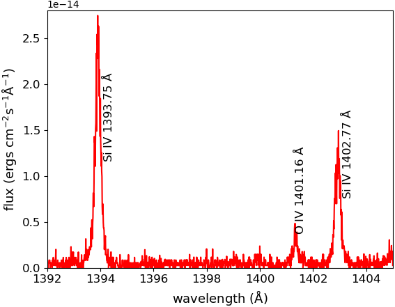
Figure 2: HST FUV spectrum of 18 Sco. The spectral lines used in this analysis are marked.

The Poynting flux to B ratio ($S_{\mathrm{A}}/B$) is a key input parameter that characterises the heating and acceleration of the wind. For a solar wind simulation using AWSoM, the $S_{\mathrm{A}}/B$ ratio was set by Sokolov et al. (2013) to be 1.1$\mathrm{\times}$ 10⁶ W m^-2 T^-1. In stellar wind modelling using AWSoM, $S_{\mathrm{A}}/B$ is sometimes adapted based on scaling laws between magnetic flux and X-ray flux (Garraffo et al., 2016; Dong et al., 2018). In this work, we investigated how the $S_{\mathrm{A}}/B$ ratio influences the mass and angular momentum loss rates, and other wind properties such as wind velocity, density, and ram pressure.

In the case of the Sun, the Alfvén wave Poynting flux $S_{\mathrm{A}}$ can be determined if we know the Alfvén speed $V_{\mathrm{A}}$ and the wave energy density $w$,

$$S_{\mathrm{A}}=V_{\mathrm{A}}w,$$ (4)

$$V_{\mathrm{A}}=B/{\sqrt{{\mu_{0}}\rho}},$$ (5)

under the assumption of equipartition of kinetic and thermal energies of Alfvén waves, the wave energy density $w$ can be expressed as,

$$w=\rho\delta{v}^{2},$$ (6)

resulting in the following $S_{\mathrm{A}}/B$ ratio,

$$S_{\mathrm{A}}/B={\rho\delta{v}^{2}}/{\sqrt{{\mu_{0}}\rho}},$$ (7)

where $\rho$ is the base density, $\delta{v}^{2}$ is the turbulent perturbation, and $\mu_{0}$ is the magnetic permeability of free space. The turbulent perturbation is related to the non-thermal turbulent velocity, $\xi^{2}=\frac{1}{2}<\delta{v^{2}}>$ (Banerjee et al., 1998). If we know the non-thermal velocity and base density for a given star, we can estimate the $S_{\mathrm{A}}/B$ ratio. Both of these quantities can be estimated using FUV spectra of stars using spectral lines that are formed in the upper chromosphere or transition region. Works by Banerjee et al. (1998), Pagano et al. (2004), Wood et al. (1997), and Oran et al. (2017) have shown that the non-thermal velocities can be determined from FUV spectral line broadening. However the $S_{\mathrm{A}}/B$ determined from FUV spectra will strongly depend on the spectral line used and can vary significantly even for the same star. Non-thermal velocities in the Sun can vary in a range of 10-30 km s^-1 (De Pontieu et al., 2007), where the distribution peaks at 15 km s^-1.

Here, we kept the base density of the solar wind constant (Table 1) and only changed the value of the non-thermal velocity in Equation 7. The non-thermal velocity was modified based on the analysis of three different spectral lines: Si IV at 1402 $\AA$, Si IV 1393 $\AA$, and O IV 1401 Å. A Hubble Space Telescope (HST) spectrum of the solar twin 18 Sco (HD146233) was used as a solar proxy (Fig. 2), instead of the Interface Region Imaging Spectrograph (IRIS) solar observations to ensure that the non-thermal velocities used in this work have similar uncertainty level as for other stars. IRIS is also not a full disk instrument although it produces full disk mosaic of the Sun once per month . The star 18 Sco was chosen as it is a well-known solar twin with a similar rotation rate as the Sun (Porto de Mello & da Silva, 1997).

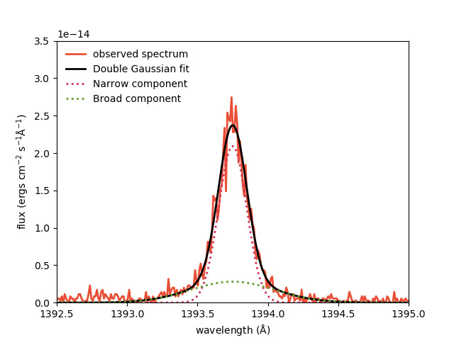
Figure 13: Double Gaussian fit of the Si IV line at 1393.75 Å.

We determined the non-thermal velocity by carrying out a double Gaussian fit to our three selected spectral lines, where the full width at half maximum (FWHM) of the narrow component of the fit gives $\xi$. The non-thermal velocity is assumed to be purely due to transverse Alfvén waves and can be used to determine the turbulent velocity perturbation $\delta{v}^{2}$(Oran et al., 2017). Figure 13 shows the Si IV line at 1393.75 Å and the the double Gaussian fit to the line. Table 2 lists the $\xi$ for each of the three spectral lines used. According to Wood et al. (1997), the narrow component of the line profile accounts for the non-thermal velocity while the broad component could be attributed to micro-flaring, though Ayres (2015) showed that the origin of the broad component is not entirely clear and could be due to chromospheric bright points (Peter, 2006). However, we note that in red giants the enhanced broadening near the wings is attributed to both radial and tangential turbulence produced by Alfvén waves (Carpenter & Robinson, 1997; Robinson et al., 1998; Airapetian et al., 2010).

We used Equation 8 to determine the non-thermal velocity from the measured FWHM (Banerjee et al., 1998; Oran et al., 2017), which is then used to determine $S_{\mathrm{A}}/B$. The FWHM is given by,

$$\mathrm{FWHM}=\sqrt{4\ln 2\left({\frac{\lambda}{c}}^{2}\right)\left(\frac{2k_{B}T_{i}}{M_{i}}+{\xi}^{2}\right)},$$ (8)

where FWHM is the full width half maximum of the narrow component of the double Gaussian fit, $\lambda$ is the rest wavelength of the spectral line in Å, $c$ is the speed of light in km s^-1, $k_{\mathrm{B}}$ is the Boltzmann constant, $M_{\mathrm{i}}$ is the atomic mass of the element, and $T_{\mathrm{i}}$ is the formation temperature in K. We fitted both single and double Gaussian line profiles and used a $\chi^{2}$ test to determine the goodness of fit. The fit is always better when a double Gaussian profile is used.

Table 2: Formation temperature and non-thermal velocity for the three FUV spectral lines and the corresponding $S_{\mathrm{A}}/B$ ratios.

spectral line	wavelength	$T_{\mathrm{i}}$	$\xi$	$S_{\mathrm{A}}/B$
	Å	K	km s-1	W m-2 T-1
Si IV	1393.75	60,000	29.6	2.2 $\times$106
Si IV	1402.77	60,000	26.6	2.0 $\times$106
O IV	1401.16	50,000	16.0	1.2 $\times$106

The non-thermal velocity determined using the O IV line is in good agreement with the peak solar non-thermal velocity of 15 km s^-1 (De Pontieu et al., 2007). The estimated $\xi$ using the Si IV lines are much higher. According to Phillips et al. (2008) the non-thermal velocity might depend on the height above the solar limb. The formation temperature of the O IV line is 50,000 K, which is also the base temperature of our simulation grid. This non-thermal velocity results in a $S_{\mathrm{A}}/B$ that is very close to the well calibrated $S_{\mathrm{A}}/B$ of Sokolov et al. (2013). The formation temperatures of the Si lines are slightly higher and lead to a higher $\xi$ as listed in Table 2. Investigation of solar non-thermal velocity at different heights by Banerjee et al. (1998) shows that the non-thermal velocity could be as high as 46 km s^-1 and changes with height. This could be linked to the damping of Alfvén waves as they move from the chromosphere to the corona due to wave reflection and dissipation. A detailed discussion on these different line formations is however beyond the scope of this work.

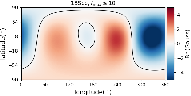
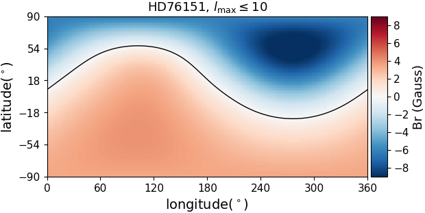
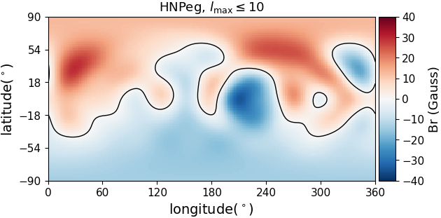
Figure 3: ZDI large-scale magnetograms of 18 Sco, HD76151, and HN Peg (top to bottom).

In the solar case, direct observations of the solar chromosphere and corona have lead to a detailed understanding of non-thermal velocities in the upper atmosphere. We can compare the non-thermal velocities obtained from FUV spectra with direct spatial observations. However, stellar observations lack the spatial and temporal resolution of the Sun. It becomes difficult to determine which out of the many non-thermal velocities available should be used to estimate $S_{\mathrm{A}}/B$. Therefore, we ran simulations of the solar wind by scaling $S_{\mathrm{A}}/B$ using the three different non-thermal velocities given in Table 2 to investigate its influence on the wind properties.

3.3 Stellar magnetic maps as a proxy for the solar magnetogram

Currently, ZDI (Semel, 1989; Brown et al., 1991; Donati & Brown, 1997; Piskunov & Kochukhov, 2002; Kochukhov & Piskunov, 2002; Folsom et al., 2018) is the only technique that can reconstruct the surface magnetic geometries of stars. It is a tomographic technique that reconstructs the large-scale magnetic geometry of stars from circularly polarised spectropolarimetric observations. It is an inverse method where a magnetic map is reconstructed by inverting observed spectropolarimetric spectra, where the surface magnetic field is described as a combination of spherical harmonic components (Donati et al., 2006) using the same equations as in Section 3.1 (see Folsom et al., 2018, for more details).

As ZDI only reconstructs the large-scale magnetic field, the magnetic maps are generally limited to $l_{\mathrm{max}}\leq 10$. As a result, the small-scale magnetic field cancel out and the global magnetic field is much weaker than in typical solar magnetograms. These ZDI magnetic maps are used as input magnetograms for stellar wind studies, where the global magnetic field strength is sometimes artificially increased to account for the loss of small-scale features. Since ZDI magnetic maps are only available for a handful of stars, it is often necessary to use a ZDI map from a star with similar parameters as a proxy, and scale it. However, the magnetic geometry of any two stars is different. Furthermore, the magnetic geometry of active Sun-like stars can evolve over very short time-scales (Jeffers et al., 2017; Rosén et al., 2016). Even the solar large-scale magnetic geometry changes complexity over the solar cycle, although the complexity of the solar magnetic field does not lead to any significant changes in the solar wind mass loss rate. It is not known if the same is true for very active Sun-like stars.

Due to the availability of observational constraints, our Sun is the best test case to investigate whether or not ZDI magnetic maps of solar analogues can be used as a solar proxy. If the simulated solar wind properties cannot be reproduced using a ZDI map of a solar analogue as a solar proxy, then it is very unlikely that the use of the Sun as a proxy for a cool star such as an M dwarf is reliable. The three solar proxies used in this work are 18 Sco, HD 76151, and HN Peg. With a rotation period of 22.7 days, 18 Sco is the only solar twin for which a large-scale ZDI surface magnetic reconstruction is available (Petit et al., 2008). HD76151 is a solar mass star and is rotating slightly faster than the Sun with a rotation period of 20.5 days (Petit et al., 2008). HN Peg is a young solar analogue and is rotating much faster than the Sun at 4.6 days (Boro Saikia et al., 2015). Table 3 lists the stellar parameters of the sample. The large-scale magnetic geometries of 18 Sco and HD76151 were reconstructed by Petit et al. (2008). The spectropolarimetric data are available as part of the open-source archive POLARBASE (Petit et al., 2014). We applied ZDI (Folsom et al., 2018) on the POLARBASE data to obtain the maps in Fig. 3. The magnetic map of HN Peg was taken from Boro Saikia et al. (2015). Figure 3 shows the large-scale radial magnetic field of the sample, where each map was reconstructed with $l_{\mathrm{max}}\leq$10.

Table 3: Stellar parameters of the sample. The masses and radii are taken from Valenti & Fischer (2005) and the rotation periods are taken from Petit et al. (2008) and Boro Saikia et al. (2015).

name	mass	radius	inclination	Prot
	M☉	R☉	∘	days
18 Sco	0.98$\pm$0.13	1.022$\pm$0.018	70	22.7
HD76151	1.24$\pm$0.12	0.979$\pm$0.017	30	20.5
HN Peg	1.085$\pm$0.091	1.002$\pm$0.018	75	4.6

We used the magnetic maps in Fig. 3 instead of an input solar magnetogram and carried out steady-state wind simulations. The other input parameters, such as $S_{\mathrm{A}}/B$, density, and temperature, were taken from Table 1.

4 Results and Discussion

4.1 Properties of the solar wind during solar cycle minimum and maximum

To determine the solar wind properties during cycle minimum and maximum, we carried out high-resolution steady state solar wind simulations (CR 2087 and CR 2159) where the input boundary conditions (Table 1) and numerical setup are the same as in van der Holst et al. (2014). The only difference is the use of a magnetogram where $l_{\mathrm{max}}$ is restricted to 150 for the input magnetic field map. Figure 4 shows the steady state solutions for the solar maximum and solar minimum cases. From the steady state solutions we determine the mass loss rate ($\dot{M}$), angular momentum loss rate ($\dot{J}$), wind velocity ($u_{\mathrm{r}}$), density ($\rho$), and ram pressure ($P_{\mathrm{ram}}$) at 1 AU. While the mass and angular momentum loss rates are discussed individually for solar cycle maximum and minimum, we combined the simulated cycle maximum and minimum data and explored the wind velocity, density, and ram pressure in terms of the fast and slow components of the wind.

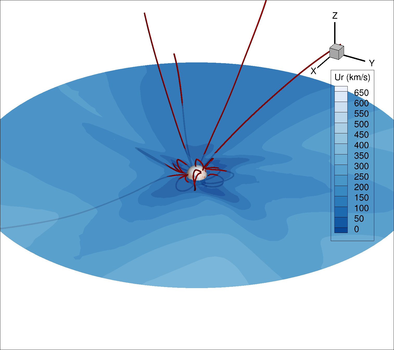
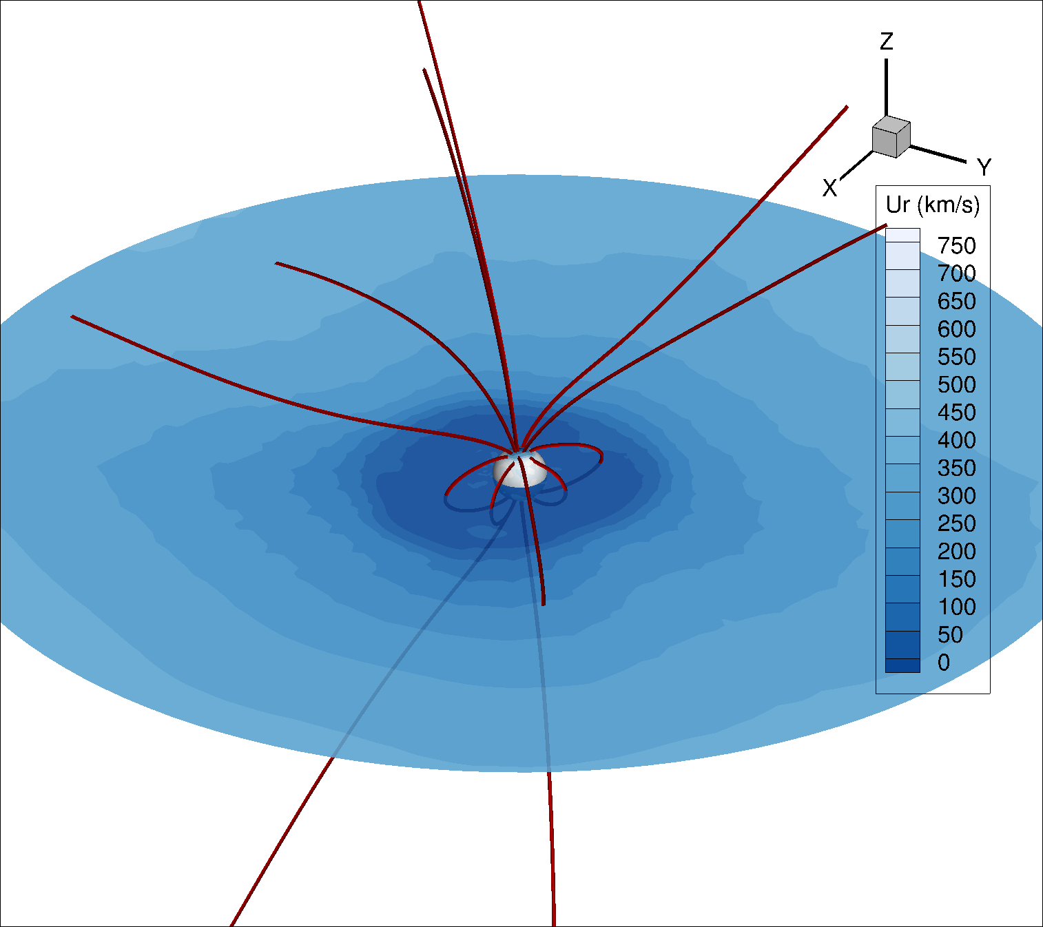
Figure 4: Steady-state simulations for the solar maximum (CR 2159, left panel) and the solar minimum (CR 2087, right panel) cases. The slice through z=0 plane shows the radial velocity. Both open and closed magnetic field lines are shown in red streamlines. The surface magnetic field geometry is shown on the solar surface as red and blue diverging contour.

The mass loss rate is determined by integrating the mass flux over a spherical surface, and is given by,

$$\dot{M}=\oint_{S}\rho u_{\mathrm{r}}\,dS,$$ (9)

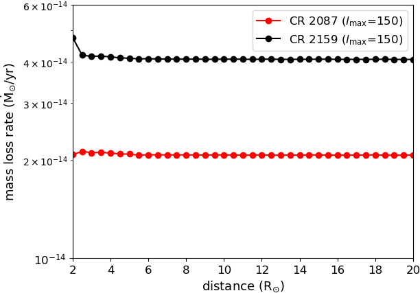
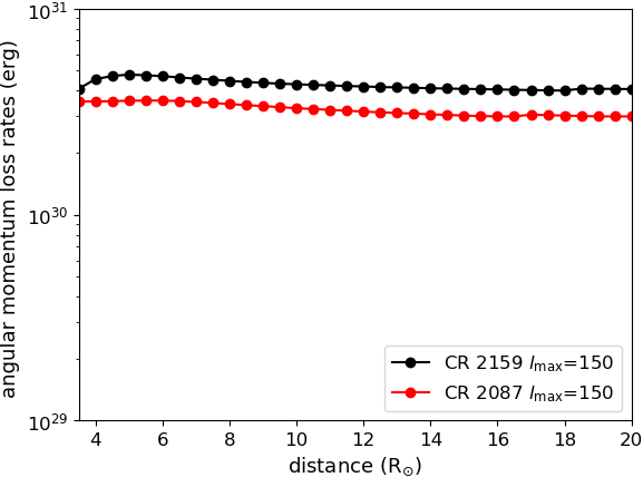
Figure 14: Mass loss (top) and angular momentum loss (bottom) rates are shown as a function of radius for both solar maximum (CR 2159, black) and solar minimum case (CR 2087, red).

where $\rho$ is the density and $u_{\mathrm{r}}$ is the radial velocity of the wind at any given distance from the solar surface. The mass loss rate of the wind is constant at any given distance from the Sun, except very close to the solar surface where not all magnetic field lines are open. The upper panel of Fig. 14 shows the mass loss rate of the wind during solar cycle maximum and minimum. The global mass loss rate is 4.1$\times$10^-14 M_☉ yr^-1 during cycle maximum and 2.1$\times$10^-14 M_☉ yr^-1 during cycle minimum. Simulations of the solar wind during solar cycle minimum and maximum by Alvarado-Gómez et al. (2016b) also agree with our results, where these later authors spatially filtered the solar magnetograms to lower their resolution. Low-resolution solar wind simulations were also carried out by Ó Fionnagáin et al. (2019) with mass loss rates one magnitude weaker than those obtained in this work. The use of different values in the input boundary conditions and different wind models could lead to such discrepancy. The mass loss rate of the Sun as observed by Ulysses and Voyager (Cohen, 2011) shows a variability of a factor of approximately two, although it is not in phase with the minimum and maximum of the solar cycle. The mass loss rates obtained from our simulations fall within the observed variation. The mass loss rates determined from our low-resolution simulations are discussed in the following section.

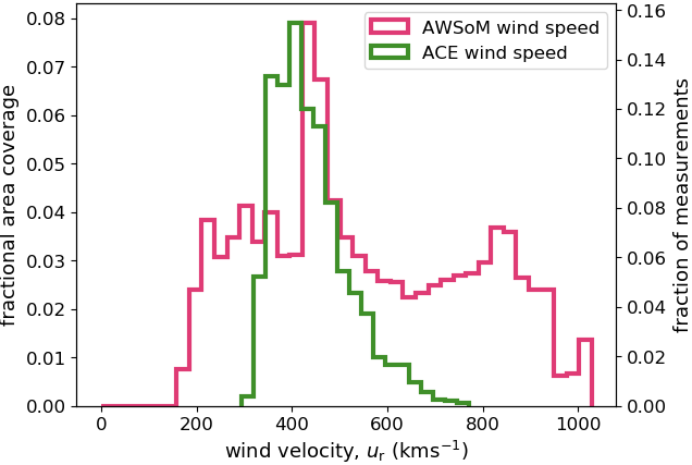
Figure 5: Simulated and observed velocity of the wind, $u_{\mathrm{r}}$ in km s^-1 at 1 AU. The combined $u_{\mathrm{r}}$ for both cycle maximum (CR 2159) and minimum (CR 2087) is shown. The ACE distribution consists of an entire year of data for CR 2159 and CR 2087. The left and right y axes show the factional area coverage of the AWSoM simulations and the fractional measurements of ACE respectively.

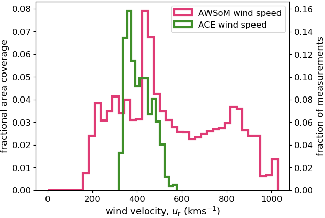
Figure 6: Same as in Fig. 5 but for ACE data containing only CR 2159 and CR 2087.

Angular momentum is carried away from the star in two forms: the angular momentum held by the wind material and angular momentum contained within the stressed magnetic field (Weber & Davis, 1967). The angular momentum loss rate is given by

$$\dot{J}=\oint_{S}\left[\frac{\varpi B_{\mathrm{\phi}}B_{\mathrm{r}}}{4\pi}+\varpi u_{\mathrm{\phi}}\rho u_{\mathrm{r}}\right]\,dS,$$ (10)

where $\varpi=\sqrt{x^{2}+y^{2}}$ is the cylindrical radius, $\rho$ is the density, $B_{\mathrm{r}}$ and $B_{\mathrm{\phi}}$ are the magnetic field components, and $u_{\mathrm{r}}$ and $u_{\mathrm{\phi}}$ are the wind velocities. The subscripts $r$ and $\phi$ represent the radial and the azimuthal direction respectively. The first component of Equation 10 is associated with the magnetic torque and the second component is the torque imparted by the plasma. As shown by Vidotto et al. (2014), Equation 10 is valid for stellar magnetic field geometries that lack symmetry. The solar magnetic field is not always axisymmetric during the solar cycle (DeRosa et al., 2012). Additionally, ZDI studies have shown that Sun-like stars often exhibit non-axisymmetric magnetic fields. For this reason, the well-known relationship of angular momentum loss rates by Weber & Davis (1967), which is only applicable for axisymmetric systems, is not used here.

During solar cycle maximum, the average AWSoM angular momentum loss is 4.0$\times$10³⁰ erg, while during cycle minimum it is 3.0$\times$10³⁰ erg (the lower panel of Fig. 14 shows the angular momentum loss rate for the Sun during solar cycle maximum and minimum). The angular momentum loss rates were obtained from the highest resolution magnetogram used in this work, $l_{\mathrm{max}}$=150. It is therefore not surprising that the angular momentum loss rate for both solar minimum and maximum is a factor of three or four higher than the angular momentum loss in Alvarado-Gómez et al. (2016b), where the authors used low-resolution, spatially filtered magnetograms. Additionally, such small differences between the results in this work and Alvarado-Gómez et al. (2016b) could also occur due to the use of different synoptic Carrington maps. The angular momentum loss rates determined using AWSoM are in strong agreement with Helios observations by Pizzo et al. (1983), although Finley et al. (2018) suggested that the angular momentum loss rate in Pizzo et al. (1983) could be underestimated due to positioning of the satellite. Our values are also within the same magnitude as those determined by Finley et al. (2018) using their open flux method. However our results are a magnitude higher than the angular momentum loss rates determined using 3D wind simulations of Finley & Matt (2018), and Réville & Brun (2017), which Finley et al. (2018) attribute to their use of a polytropic equation of state instead of Alfvén wave heating.

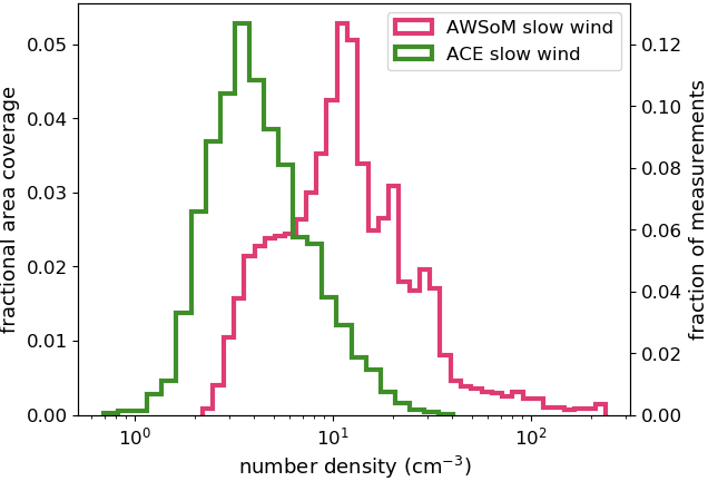
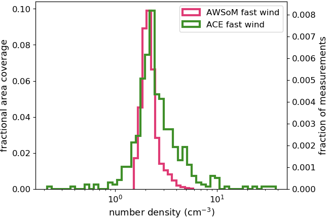
Figure 7: Simulated and observed proton number densities for both slow (top) and fast (bottom) component of the wind at 1 AU. The left y-axis represents fractional area coverage of our AWSoM simulations and the right y-axis represents the fraction of ACE measurements.

We combined the wind output of the two steady-state simulations (solar maximum and minimum) to study wind properties such as velocity, proton density, and ram pressure as a function of the observed ACE wind properties. Distribution of wind velocity $u_{\mathrm{r}}$ at a distance of 1 AU for combined solar cycle minimum (CR 2087) and maximum (CR 2159) are shown in Fig. 5. The IH component of the simulation grid was invoked to generate the wind properties at that distance. The distribution of the hourly averaged ACE solar wind speeds during the same years as CR 2159 and CR 2087 is also shown in Fig. 5. The full two years containing CR 2159 and CR 2087 are combined to obtain the ACE distribution in Fig. 5. The fast wind cutoff is made at $u_{\mathrm{r}}$=600 km s^-1 in this work. The simulated slow wind peak is in good agreement with the observed ACE slow wind peak.

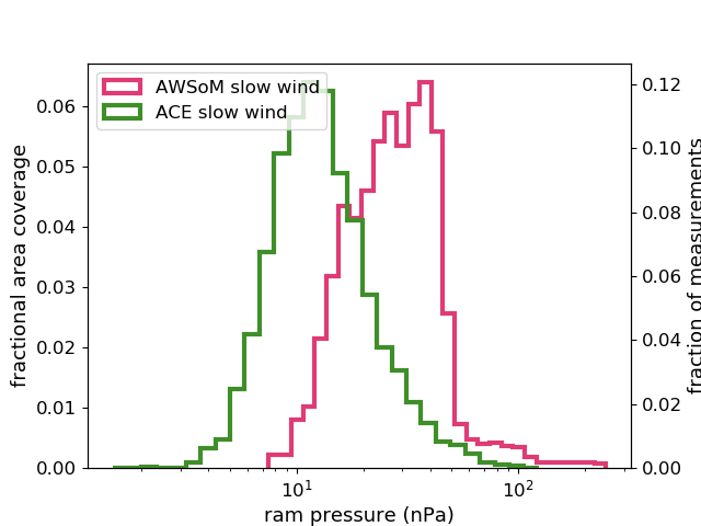
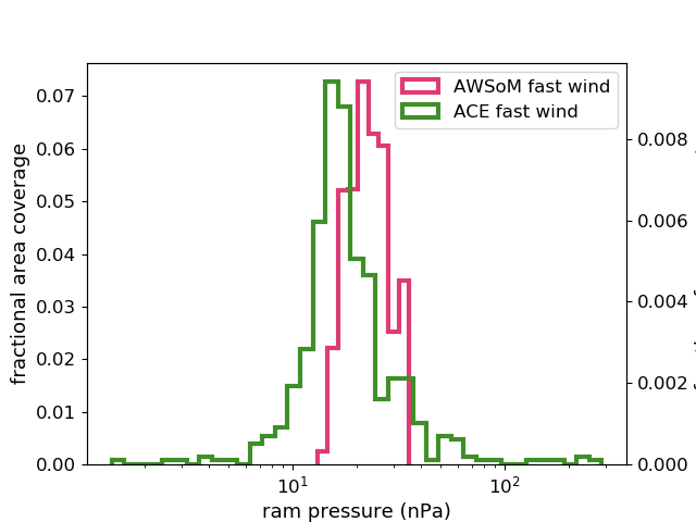
Figure 8: Simulated and observed ram pressures due to the slow (top) and fast (bottom) components of the solar wind for the combined cycle maximum and minimum simulations. The left y-axis shows the fractional area coverage of the AWSoM simulations and the right y-axis shows the fraction of ACE measurements.

Since the observations were taken by ACE, the distribution in Fig. 5 is biased towards the slow wind component. The ACE satellite is positioned at L1 in the equatorial plane and therefore mostly measures the slow component of the wind. Ulysses measures both the slow and the fast component of the wind, but only limited measurements are available for the year that CR 2087 took place, during which time it was situated close to the equatorial plane. Ulysses has no measurements from CR 2159. Multi-year observations taken by Ulysses show that the fast wind speed is in good agreement with our results. The median Ulysses fast and slow wind speeds of 760 km s^-1 and 400 km s^-1 (Johnstone et al., 2015b) are very similar to our median fast and slow wind speeds of 794 km s^-1 and 391 km s^-1 respectively. The median fast wind speed of ACE is 639 km s^-1; however, this value could be biased because ACE does not have many observations of the fast wind. The median ACE wind speed is determined using all available data of the two years containing CR 2159 and CR 2087. Figure 6 shows the hourly averaged ACE wind velocities, where only CR 2159 (January 2015) and CR 2087 (August 2009) data are included. The entire AWSoM distribution from Fig. 5 is also shown. During this period, no fast wind component was recorded by ACE. Therefore, we use all the data from the years that contain CR 2159 and CR 2087 (Fig. 5) to compare the model with observations of both slow and fast wind.

The proton density of the solar wind at a distance of 1 AU for the combined solar cycle maximum (CR 2159) and minimum (CR 2087) simulations is shown in Fig. 7. The density of the slow wind is shown in the upper panel and the fast wind is shown in the lower panel. The ACE proton density for the fast and slow wind is also shown in Fig 7. The proton density of the fast wind is lower than the proton density of the slow wind in our simulations, which is also seen in ACE observations. However very high slow wind proton densities are obtained in our simulations, which are not seen in the ACE data. The median proton density of the slow wind in our simulations is 12.7 cm^-3, which is about three times higher than the median ACE slow wind density (4.0 cm^-3). The agreement between AWSoM and ACE fast wind densities is better when compared to the slow wind. The median fast wind proton density in our simulations is 2.1 cm^-3 and the median ACE fast wind density is 2.3 cm^-3, although only very limited ACE fast wind measurements are available.

We also calculated the ram pressure due to the solar wind as it is the dominant pressure component at a distance of 1 AU. The shape of planetary magnetospheres in the habitable zone of a Sun-like star strongly depends on the wind ram pressure. The ram pressure due to the solar wind is calculated based on the following equation,

$$P_{\mathrm{ram}}=\rho u_{\mathrm{r}}^{2},$$ (11)

where $\rho$ is the wind density in g cm^-3 and $u_{\mathrm{r}}$ is the wind radial velocity in km s^-1.

Figure 8 shows the ram pressure $P_{\mathrm{ram}}$ distribution in nPa at a distance of 1 AU for both slow (Fig. 8, upper panel) and fast components (Fig. 8, lower panel) of the wind. The ram pressure calculated from ACE density and velocity measurements is also shown. There is no significant difference in the ram pressure for the slow and the fast wind. As density and wind speed have an inverse relation, they balance out in Equation 11, resulting in similar contributions from both the fast and the slow wind components. The slight discrepancy in the ram pressure distribution between observations and simulations is most likely due to the high velocities ($\sim$ 1000 km s^-1) of the fast wind component around the polar regions in the AWSoM simulations. No polar observations of the solar wind exist to date, except for a few polar coronal hole measurements by Ulysses. It is therefore difficult to conclude how realistic the simulated polar wind speeds are. The AWSoM simulations lead to a median ram pressure of 31.8 nPa for the slow wind, which is higher than the ACE median ram pressure (12.4 nPa) by a factor of about 2.5. The median AWSoM ram pressure for the fast wind in the simulations is 22.3 nPa, while the ACE observations lead to a median ram pressure of 17.2 nPa.

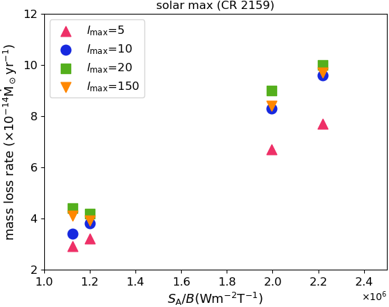
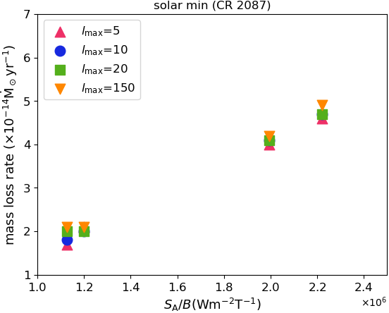
Figure 9: Mass loss rate for the grid of simulations during cycle maximum (CR 2159) (left) and minimum (CR 2087) (right). The different colours represent different values of $l_{\mathrm{max}}$.

The discrepancies between simulated AWSoM and observed ACE wind velocities and proton densities could have several causes. It is well known in the solar community that although there is a general consensus between magnetograms from different solar observatories, there are still some discrepancies between their synoptic magnetic maps (Riley et al., 2014). Based on the choice of solar observatory for the input magnetogram, the final wind output could also vary (Gressl et al., 2014). Furthermore we cannot reliably observe the polar magnetic field and the polar field in the magnetograms is usually based on empirical models. This could also explain the very high wind velocities at the polar regions obtained in our simulations. Table 4 shows the median and mean solar wind properties during cycle minimum and maximum for the high-resolution solar wind simulations with $l_{\mathrm{max}}$=150 and $S_{\mathrm{A}}/B$=1.1 $\times$10⁶ W m^-2 T^-1. Caution should be taken regarding the fast wind properties of ACE as the satellite did not take enough observations of the fast component of the wind for the results to be statistically significant.

Table 4: Median and mean values of the wind speed, proton density, and ram pressure for the slow and the fast wind of both AWSoM simulations ($l_{\mathrm{max}}$=150 and $S_{\mathrm{A}}/B$=1.1$\times$10⁶ W m^-2 T^-1) and ACE observations.

	Median $u_{\mathrm{r}}$	Mean $u_{\mathrm{r}}$	Median $n_{\mathrm{p}}$	Mean $n_{\mathrm{p}}$	Median $P_{\mathrm{ram}}$	Mean $P_{\mathrm{ram}}$
	km s-1	km s-1	cm-3	cm-3	nPa	nPa
			slow wind
AWSoM	391	380	12.7	20.3	31.8	35.3
ACE	420	430	4.0	5.1	12.4	15.0
			fast wind
AWSoM	794	790	2.1	2.2	22.3	23.0
ACE	639	647	2.3	3.2	17.2	21.9

4.2 Solar wind properties determined from our two grids of low-resolution simulations

The two 4$\times$4 grids of simulations were created by altering the two key input parameters $l_{\mathrm{max}}$ and $S_{\mathrm{A}}/B$. The $S_{\mathrm{A}}/B$ value of 1.1 $\times$10⁶ W m^-2 T^-1 is the solar $S_{\mathrm{A}}/B$ taken from Sokolov et al. (2013). The other three values of $S_{\mathrm{A}}/B$ were determined from the HST spectra of 18 Sco. The other input parameters listed in Table 1 were kept constant. The two grids represent solar cycle maximum (CR 2159) and minimum (CR 2087).

Figure 9 shows the mass loss rate for our two 4$\times$4 grids. During solar cycle maximum (left panel of Fig. 9), the mass loss rate changes by a factor of $\leqslant$ 1.5 over a range of $l_{\mathrm{max}}$ for a given $S_{\mathrm{A}}/B$. For example, keeping $S_{\mathrm{A}}/B$ constant at 1.1 $\times$10⁶ W m^-2 T^-1 and only changing the $l_{\mathrm{max}}$, the difference in the mass loss rate between the four simulations is a factor of about 1.5. However, if we keep $l_{\mathrm{max}}$ constant and use different values of $S_{\mathrm{A}}/B$, the mass loss rate can differ by a factor approximately 3. For the set of simulations where $l_{\mathrm{max}}$=5, the mass loss rate changes by a factor of 2.6 over a range of $S_{\mathrm{A}}/B$. During solar cycle minimum (Fig. 9, right), the mass loss rate shows almost no variability for different values of $l_{\mathrm{max}}$ at a constant $S_{\mathrm{A}}/B$. The mass loss rate changes by a factor of about 2.7 or less for simulations with a constant $l_{\mathrm{max}}$ and varying $S_{\mathrm{A}}/B$.

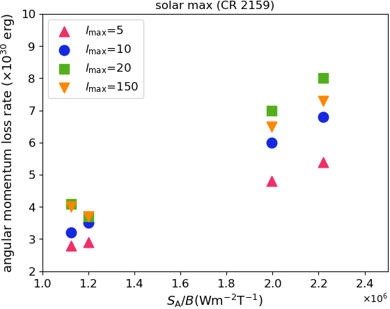
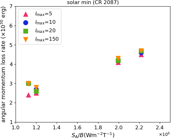
Figure 10: Same as Fig. 9 except the angular momentum loss rate is shown instead of the mass loss rate.

Our results show that, depending on the activity level of the Sun, the resolution ($l_{\mathrm{max}}$) of the magnetic map has a small or negligible influence on the mass flux. During solar cycle maximum, the mass loss rate has a stronger dependence on the resolution (Table 5) than during solar cycle minimum. Almost no variation is detected in the simulated mass loss rates during solar cycle minimum (Table 6). The mass flux has a much stronger dependence on the $S_{\mathrm{A}}/B$ instead of $l_{\mathrm{max}}$. Irrespective of the solar activity cycle, the mass loss rate changes by a factor of between two and three over a range of $S_{\mathrm{A}}/B$ at a given $l_{\mathrm{max}}$.

The angular momentum loss rate for the two grids during solar cycle maximum and minimum are shown in Fig. 10. The variability in angular momentum loss for different values of $l_{\mathrm{max}}$ at a constant $S_{\mathrm{A}}/B$ during cycle maximum is a factor of $\leqslant$1.5. The variability increases to a factor of about 2 for different values of $S_{\mathrm{A}}/B$ at a constant $l_{\mathrm{max}}$ (Table 5). During solar cycle minimum, the angular momentum shows negligible variations over a range of $l_{\mathrm{max}}$ at a constant $S_{\mathrm{A}}/B$; it varies by a factor of $\leqslant$ 1.9 over a range of $S_{\mathrm{A}}/B$ at a constant $l_{\mathrm{max}}$. The angular momentum loss shows similar dependence on $l_{\mathrm{max}}$ and $S_{\mathrm{A}}/B$ to the mass loss rate. Tables 5 and 6 show the mass loss and the angular momentum loss rates for the two grids during cycle maximum and minimum respectively.

The mass loss and angular momentum loss rates show a slight decrease as the resolution lowers, as shown in Figs. 9 and 10. This could be attributed to the loss of small-scale magnetic features for low values of $l_{\mathrm{max}}$, resulting in a simpler field geometry. According to Wang & Sheeley (1990), the expansion of flux tubes from the photosphere to the corona determines the wind density, temperature, velocity, and mass flux. The higher the expansion factor, the stronger the wind mass loss rate. The expansion factor increases for small-scale features which is another explanation for stronger mass loss rates for higher values of $l_{\mathrm{max}}$. Furthermore, higher $l_{\mathrm{max}}$ also leads to stronger surface magnetic field, which leads to higher heating at the base leading to more mass loss. The higher expansion factor during solar cycle maximum, when the number of small-scale features is higher, could also explain the increase in mass loss rate for CR 2159.

The impact of stellar magnetogram resolution was also investigated by Jardine et al. (2017), who lowered the resolution of solar magnetograms using the same method as used in this work and used an empirical wind model to establish that the mass and angular momentum loss rates for a low-resolution magnetogram are within 5-20 $\%$ of the full resolution value. Since the large-scale dipole field is the key driver of mass and angular momentum loss in Sun-like stars, the resolution loss in ZDI does not have a significant influence on the mass or angular momentum loss rates (Réville et al., 2015; See et al., 2018). However, the resolution of the magnetogram might have a stronger impact for slowly rotating stars with Rossby number  2 (See et al., 2019).

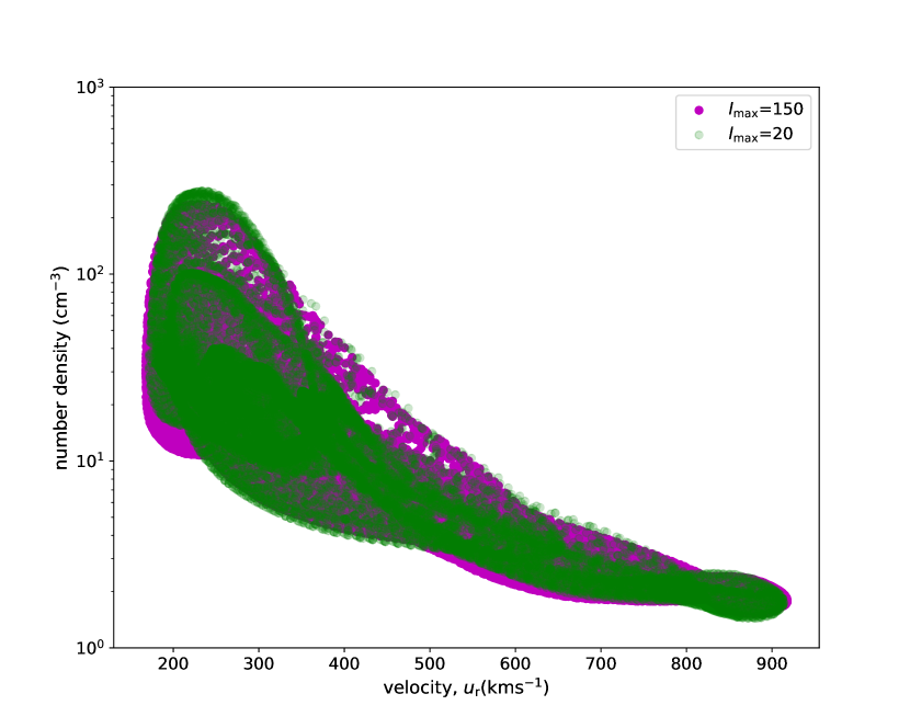
Figure 15: Proton number density vs. wind velocity, $u_{\mathrm{r}}$ during solar maximum, CR 2159. The $l_{\mathrm{max}}$=150 simulation is shown in magenta and $l_{\mathrm{max}}$=20 simulation output is shown in green.

Surprisingly, $l_{\mathrm{max}}$=20 leads to a marginally higher mass loss and angular momentum loss rate when compared to $l_{\mathrm{max}}$=150 during solar cycle maximum in CR 2159. As $l_{\mathrm{max}}$=150 has more closed small-scale magnetic regions it is expected to have the strongest mass and angular momentum loss. As shown in Equation 9, $\dot{M}$ depends on the wind velocity $u_{\mathrm{r}}$ and density $\rho$. As the solar wind moves outwards, the velocity increases and the number density decreases. Figure 15 shows that during solar cycle maximum, the number density is slightly higher for $l_{\mathrm{max}}$=20 compared to $l_{\mathrm{max}}$=150. This could explain the slightly higher mass loss rate for $l_{\mathrm{max}}$=20.

The $S_{\mathrm{A}}/B$ has a stronger influence on the wind mass loss and stellar angular momentum loss compared to the choice of $l_{\mathrm{max}}$. This is not surprising since the Alfvén wave energy determines the heating and acceleration of the wind in the AWSoM model. This shows that robust determination of $S_{\mathrm{A}}/B$ is important for strong magnetic fields with complex field geometries. Our results also show that the O IV line is a good tracer for $S_{\mathrm{A}}/B$ scaling. However, further investigations are needed to determine its suitability for other stars.

As the variation in mass loss and angular momentum loss is not significant over the given range of $l_{\mathrm{max}}$, we investigated how the wind speed, proton number density, and ram pressure are affected for the different values of $S_{\mathrm{A}}/B$ in Table 2. We used the lowest ($l_{\mathrm{max}}$=5) and the highest ($l_{\mathrm{max}}$=150) resolution magnetograms for this purpose. These three wind properties for the fast and slow wind are determined from the combined solar maximum and minimum simulations.

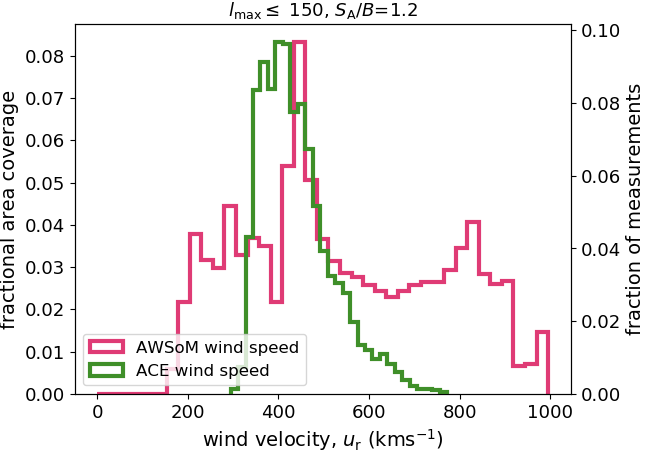
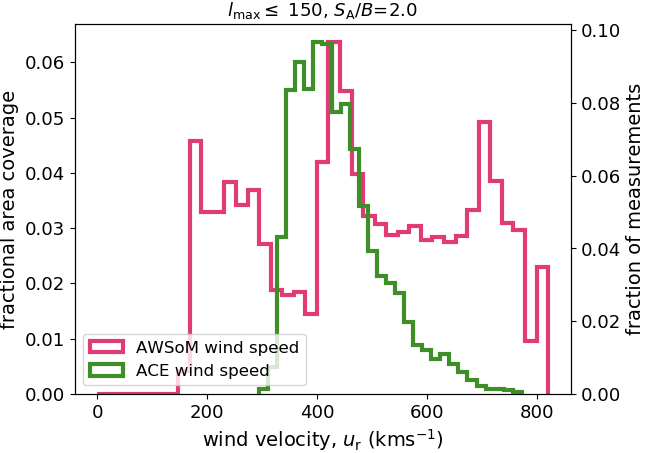
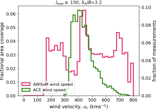
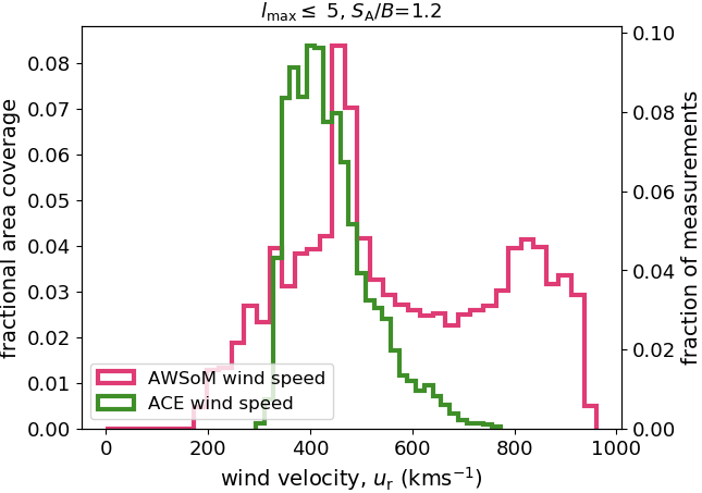
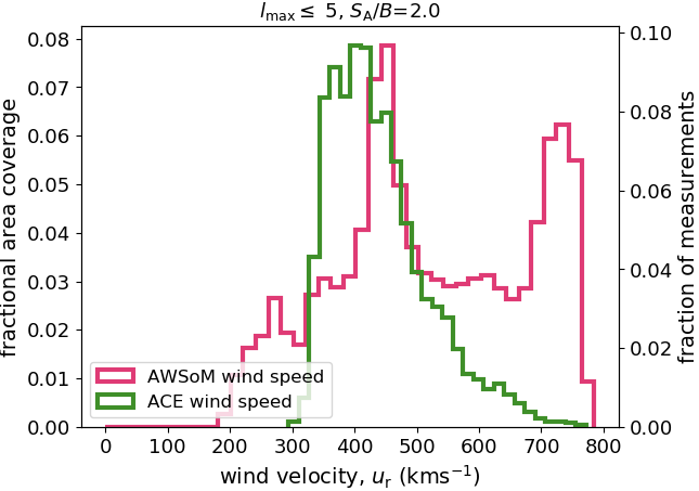
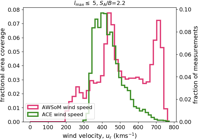
Figure 16: Distribution of wind velocity at 1 AU for a subset of our simulations during solar cycle minimum and maximum. Each column represents a steady state simulation for different values of $S_{\mathrm{A}}/B$. The resolution of the magnetogram is truncated to $l_{\mathrm{max}}$=150 (top) and $l_{\mathrm{max}}$=5 (bottom). ACE data is shown in green.

Figure 16 shows the wind speed for different values of $S_{\mathrm{A}}/B$ at $l_{\mathrm{max}}$=150 (upper panel) and $l_{\mathrm{max}}$=5 (lower panel), respectively. As expected, the distribution of the wind velocity is almost consistent for the high-resolution ($l_{\mathrm{max}}$=150) and the low-resolution ($l_{\mathrm{max}}=5$) simulations. The wind velocity shows a considerable variation with a varying $S_{\mathrm{A}}/B$. As the $S_{\mathrm{A}}/B$ increases the wind velocity of the fast wind decreases, while the slow component does not show any considerable change in wind speeds. Table 7 and 8 show the median and mean wind velocities at a distance of 1 AU for the distributions shown in Fig. 16.

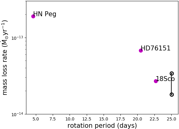
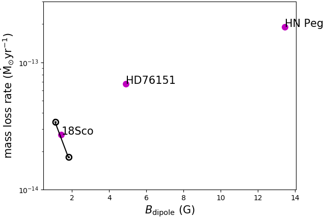
Figure 11: Solar mass loss rate for different ZDI input magnetograms, shown in magenta, as a function of rotation period (left) and dipolar field strength in Gauss (right). Solar symbols connected by the black vertical line shows the mass loss rate for the solar input magnetograms ($l_{\mathrm{max}}$=10) during solar cycle minimum and maximum.

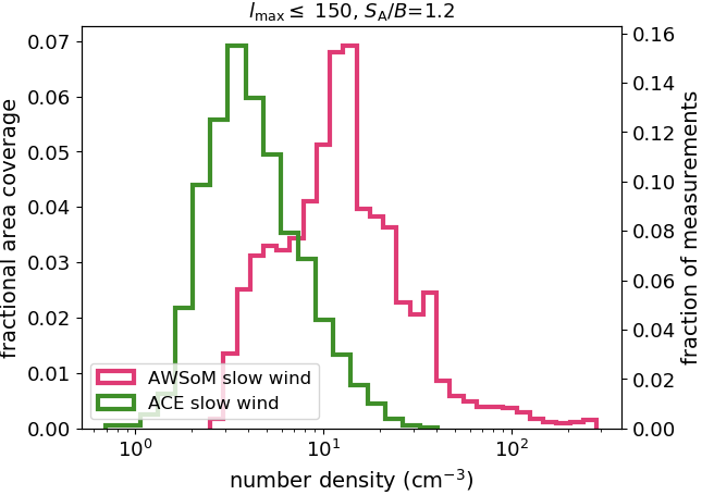
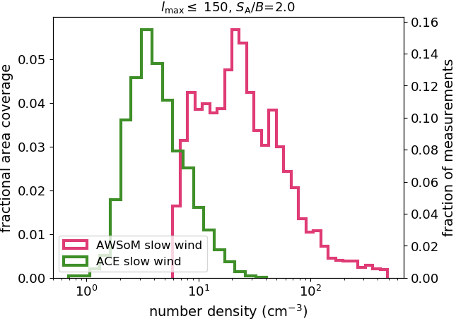
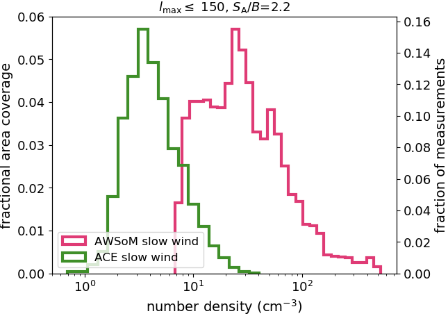
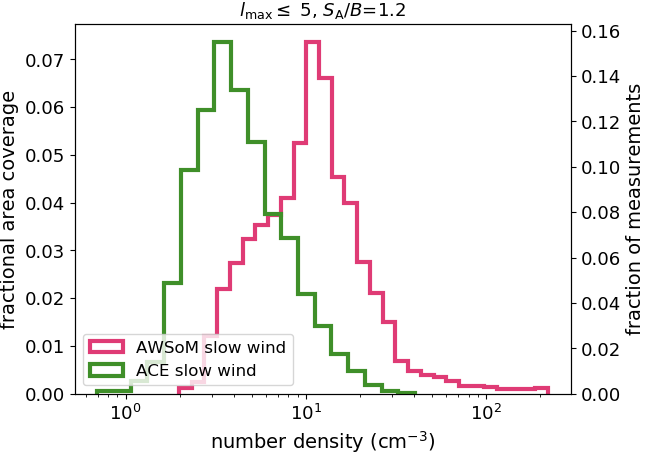
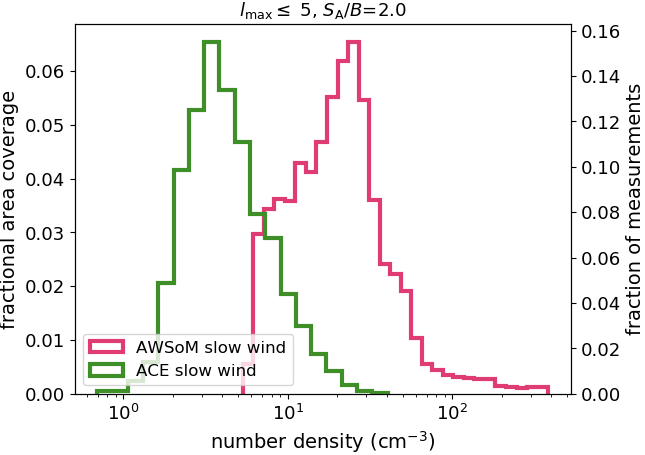
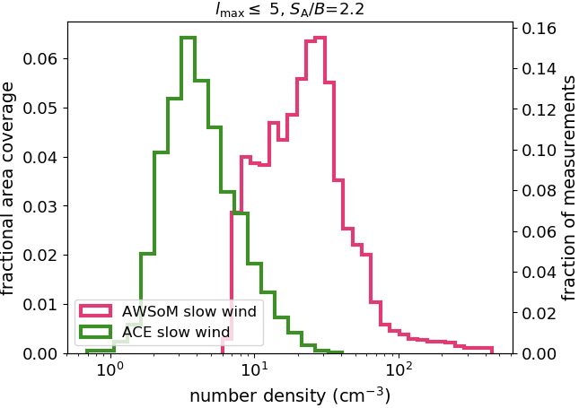
Figure 17: Proton number density of the slow wind for the same simulations as in Fig .16. The observed ACE proton densities are shown in green.

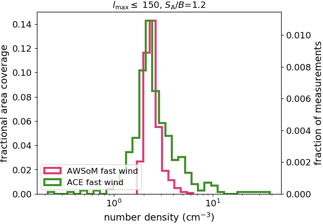
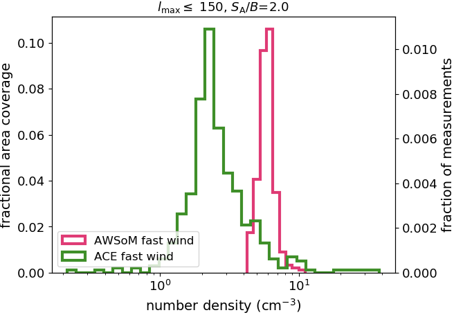
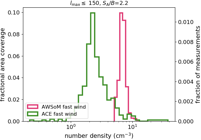
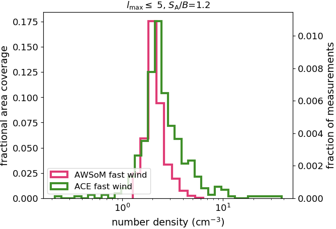
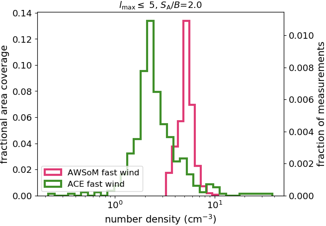
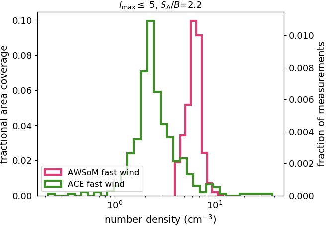
Figure 18: Same as in Fig. 17 but for the fast wind.

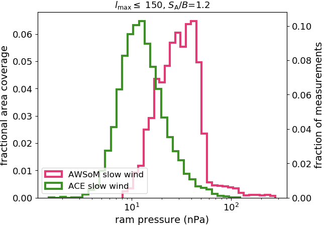
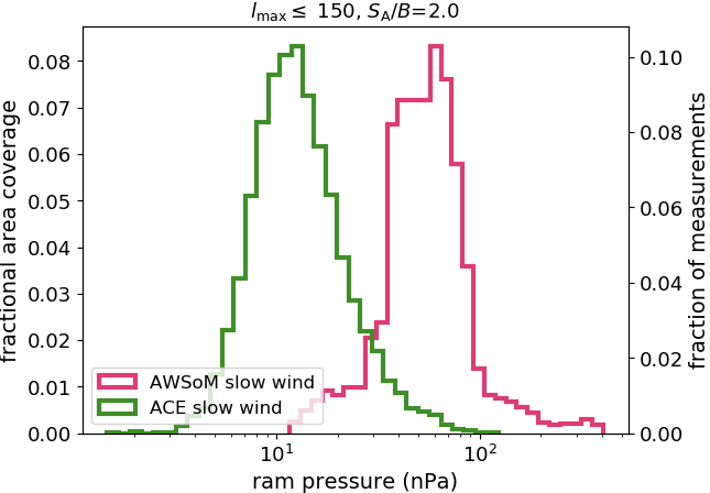
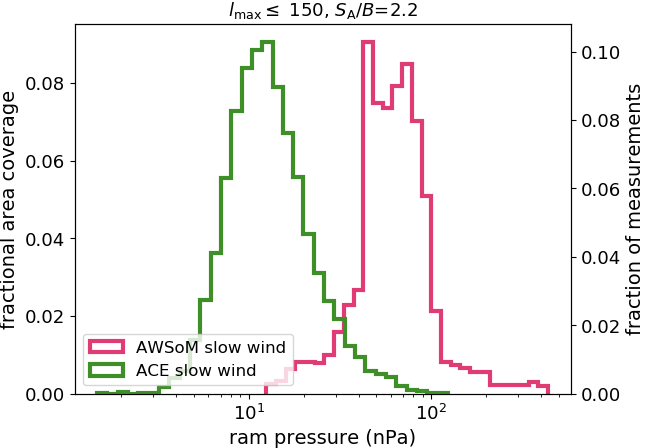
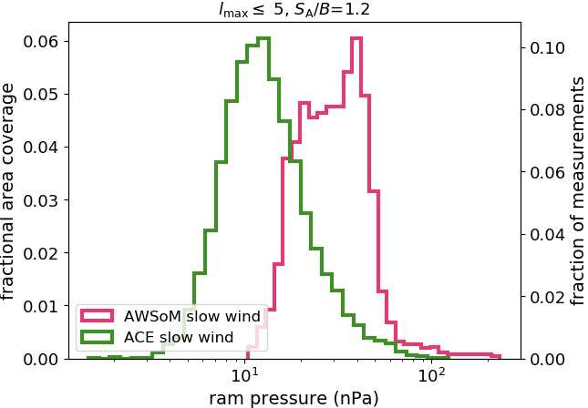
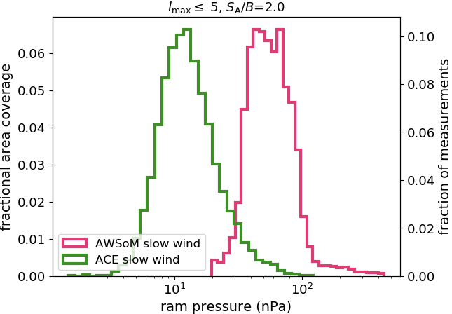
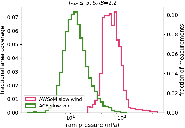
Figure 19: Ram pressure for the same simulations as in Fig. 16. ACE ram pressure is shown in green.

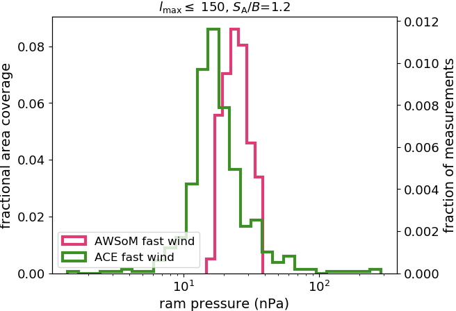
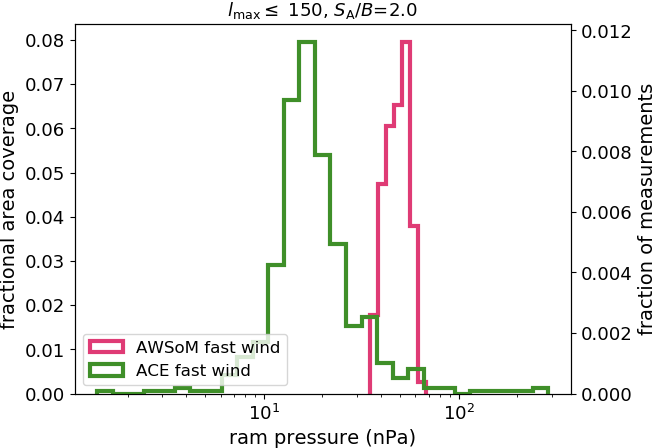
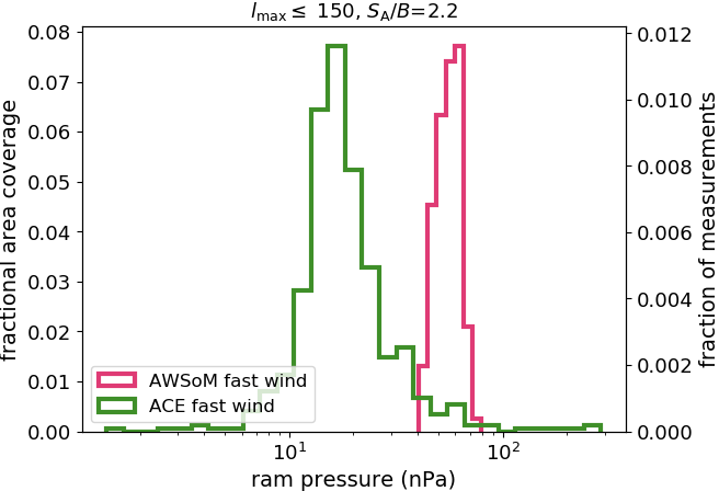
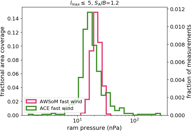
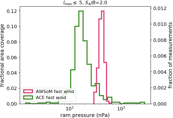
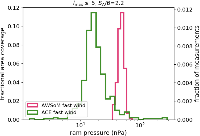
Figure 20: Same as in Fig. 19 but for the fast wind.

The proton density distribution of the slow and fast wind for $l_{\mathrm{max}}$=150 and 5 over a varying $S_{\mathrm{A}}/B$ is shown in Figs. 17 and 18 respectively. The proton density for both slow fast wind increases with increasing $S_{\mathrm{A}}/B$. The density increases by a factor of approximately two from $S_{\mathrm{A}}/B$=1.2 to 2.2. The median and mean values are shown in Table 7 and 8. The ram pressure shows a similar trend to the proton density distribution, as shown in Figs. 19 and 20; it also shows a variation by a factor of approximately two depending on the choice of $S_{\mathrm{A}}/B$. Although the mean and median wind velocity are not strongly influenced by the choice of $S_{\mathrm{A}}/B$, the density varies by a factor of about two, resulting in a corresponding change in ram pressure. The median and mean values of the ram pressure are tabulated in Tables 7 and 8. Our results show that, similar to the mass loss and angular momentum loss rates, the density and ram pressure are more influenced by the $S_{\mathrm{A}}/B$ than by the resolution. Although the mean and median wind velocities are not strongly impacted by the variation of either $S_{\mathrm{A}}/B$ or $l_{\mathrm{max}}$, the distribution of the fast wind shows some dependence on $S_{\mathrm{A}}/B$. For the solar case the variation is a factor of between two and three, but it could be much higher for a more active star.

4.3 Solar wind properties determined using ZDI stellar magnetograms

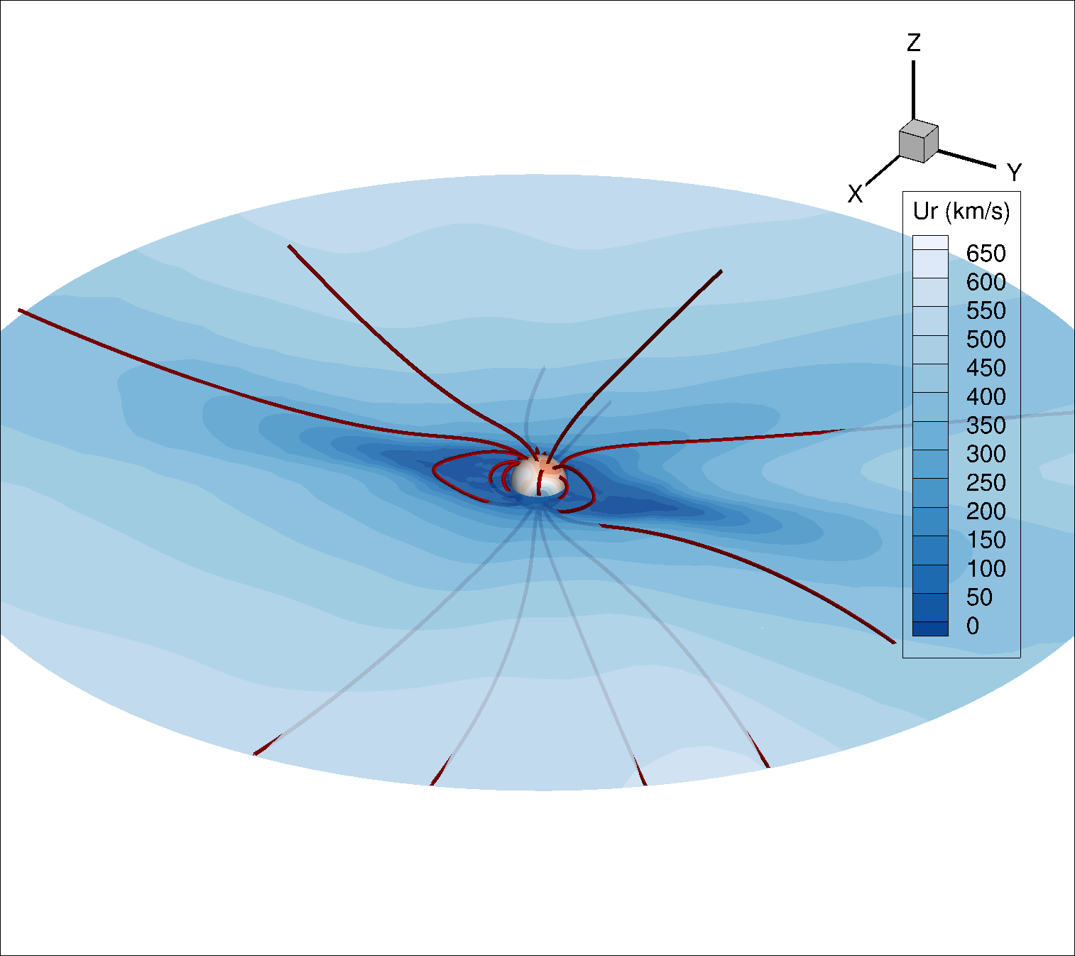
Figure 21: Same as Fig. 4 but for HN Peg.

One problem often faced in stellar wind modelling is the lack of stellar magnetograms, as ZDI stellar magnetic maps are only available for $<$ 100 stars. To circumvent this problem, solar magnetograms are sometimes used as a proxy for the stellar magnetic field in stellar wind modelling (Dong et al., 2018). Unfortunately it is not known whether or not such approximations introduce any additional biases in the simulated wind properties. We investigated if the solar wind properties can be reproduced if we use ZDI magnetograms of Sun-like stars as the input for the solar magnetic field. This will allow us to have some insight into the usability of a magnetic map from one star (or even the sun) for a study of the wind properties of another. We used large-scale ZDI magnetic maps of three solar analogues as a proxy for the solar magnetogram to carry out AWSoM solar wind simulations. The ZDI maps were used instead of the GONG magnetograms used in the previous section. Solar input boundary conditions are used, which are the same values as listed in Table 1. Figure 21 shows the velocity distribution of a steady-state simulation of one of the solar proxies HN Peg.

Figure 11 shows the mass loss of the solar wind for three different input ZDI magnetic maps reconstructed with maximum spherical harmonic degree $l_{\mathrm{max}}$=10. The solar mass loss rate during cycle maximum (CR 2159) and minimum (CR 2087) for $l_{\mathrm{max}}$=10 and $S_{\mathrm{A}}/B$=1.1 $\times$10⁶ W m^-2 T^-1 is also shown. When a magnetic map of 18 Sco is used as a solar proxy, the mass loss rate is in good agreement with the solar mass loss rate. The AWSoM solar wind simulation, where the solar magnetogram is replaced by a large-scale magnetic map of the solar analogue HD76151, results in a mass loss rate that is more than three times the solar mass loss rate at cycle minimum. Finally, the AWSoM simulation, where a large-scale magnetic map of the young solar analogue HN Peg is used as the input magnetogram, leads to a mass loss which is approximately ten times higher than the solar mass loss.

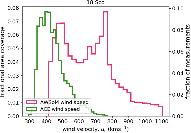
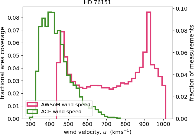
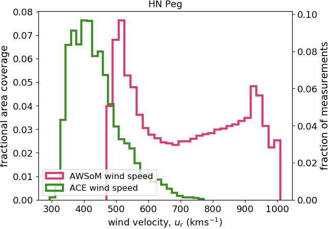
Figure 22: Wind velocity determined from ZDI simulations of the three stars: 18 Sco, HD 76151, HN Peg (left to right) in magenta. The observed ACE wind velocities are shown in green.

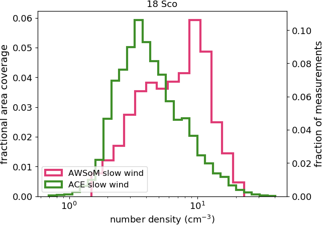
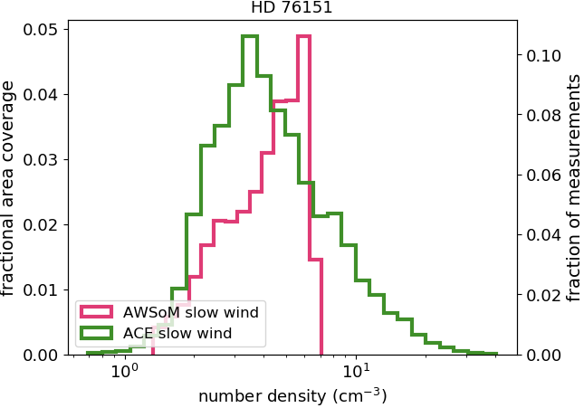
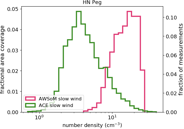
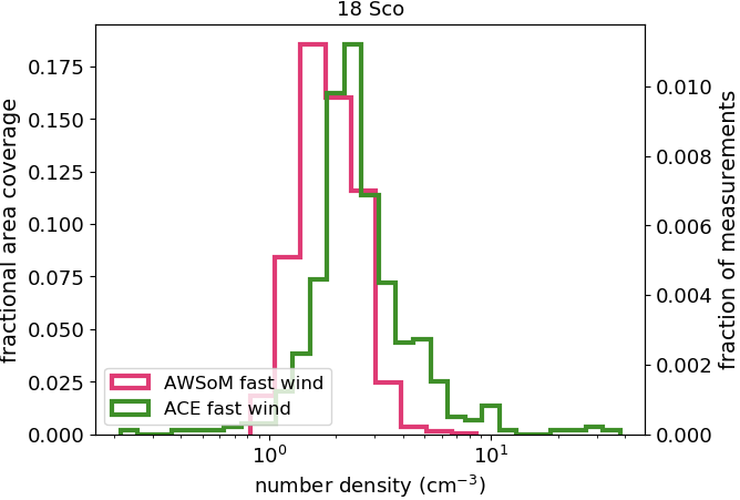
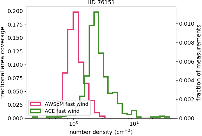
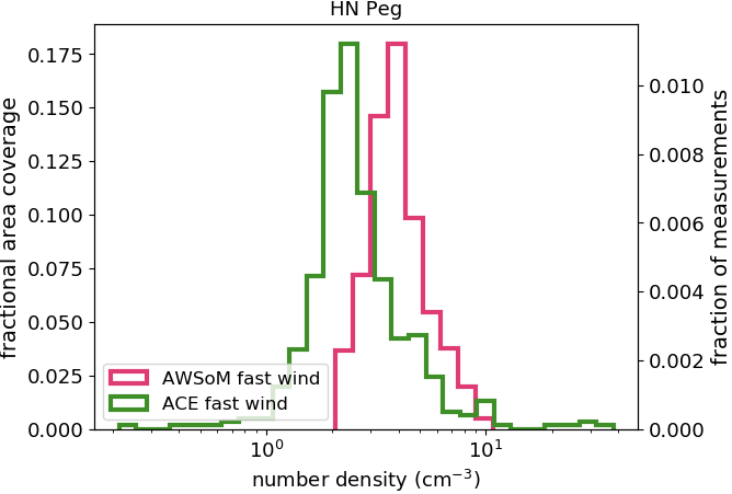
Figure 23: Proton number density for the slow (top) and fast (bottom) component of the wind. Each column represents wind simulations for the three stars included in this work: 18 Sco, HD76151, HN Peg (left to right, magenta). ACE proton density is shown in green.

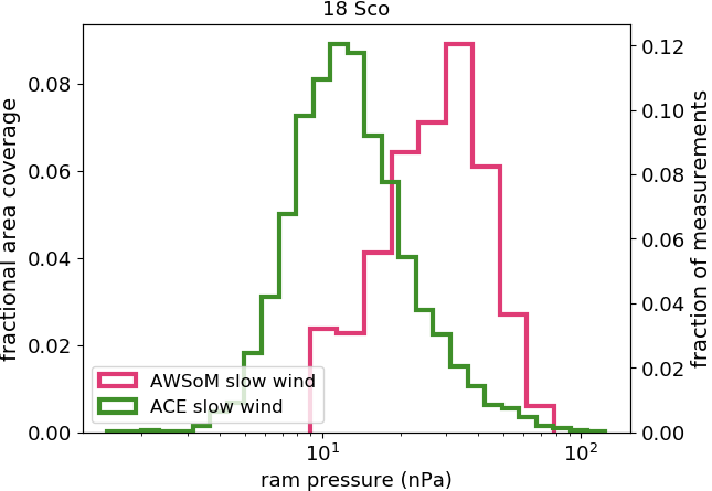
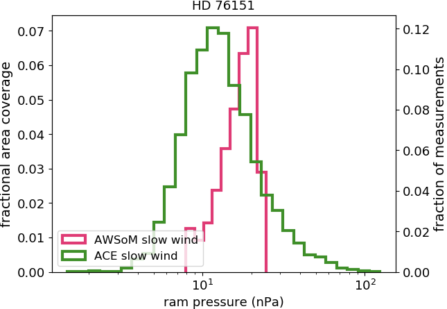
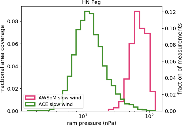
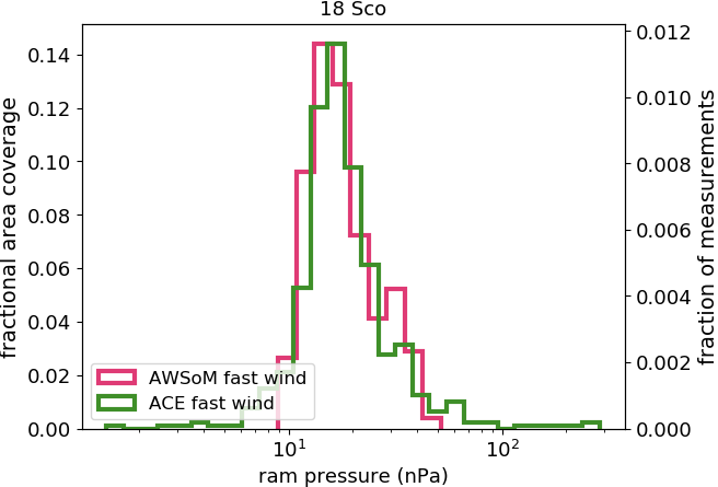
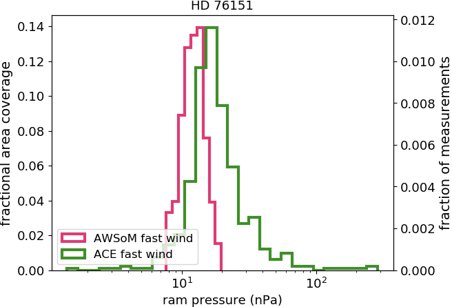
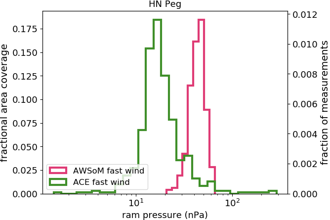
Figure 24: Same as in Fig. 23 except the ram pressure is shown instead of the proton density.

The angular momentum loss due to the solar wind, where these three ZDI large-scale magnetograms are used as input, is shown in Fig. 12. The angular momentum loss rate of the Sun during cycle maximum and minimum where a magnetogram with $l_{\mathrm{max}}$=10 and $S_{\mathrm{A}}/B$=1.1 $\times$10⁶ W m^-2 T^-1 is used is also shown in Fig. 12. For both 18 Sco and HD76151 input magnetic maps, the angular momentum loss is within one magnitude of the solar simulations in Fig. 12. However, there is a factor of approximately ten difference between the HN Peg simulations and the solar simulations in the previous section. Discrepancies in wind velocity, density, and ram pressure between ACE observations and the three ZDI simulations are also detected, as shown in Figs. 22, 23, and 24.

Our results show that the large-scale magnetic map of the solar twin 18 Sco is a good solar proxy for wind simulations. The mass loss rate agrees strongly with both observed mass loss rates and our simulated mass loss rates for different values of $l_{\mathrm{max}}$. The angular momentum loss is a factor of three lower than our simulations that use $l_{\mathrm{max}}$=10 and $S_{\mathrm{A}}/B$=1.1 $\times$10⁶ W m^-2 T^-1, and also the values obtained from Helios observations (Pizzo et al., 1983). However, it falls within the range of angular momentum loss rates determined by Finley et al. (2018) over the solar cycle. The dipole field strength of 18 Sco is similar to the solar dipolar field strength. The dipolar component is primarily responsible for the wind mass loss and angular momentum loss (Réville et al., 2015). HD76151 rotates at 20.5 days and when used in a solar wind simulation results in mass and angular momentum loss rates that are higher than those of 18 Sco. The mass loss rate agrees very well with cycle maximum solar wind simulations in the previous section where $S_{\mathrm{A}}/B$= 2.0 $\times$10⁶ W m^-2 T^-1. HD76151 has a stronger dipolar field when compared to the dipolar magnetic fields of both the Sun and 18 Sco. This could explain the mass and angular momentum loss rates being slightly higher than the solar magnetogram simulations for $l_{\mathrm{max}}$=10 and $S_{\mathrm{max}}/B$=1.1 $\times$10⁶ W m^-2 T^-1.

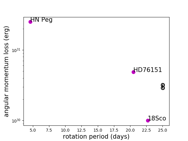
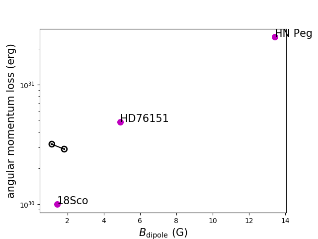
Figure 12: Same as Fig. 11, except the angular momentum loss rate is shown instead of the mass loss rate.

Unsurprisingly, the strongest mass and angular momentum loss rates are obtained for an input magnetogram of the young solar analogue HN Peg. The mass and angular momentum loss rates are a factor of approximately ten stronger than the solar cycle minimum mass and angular momentum loss rates (simulation carried out using $l_{\mathrm{max}}$=150, $S_{\mathrm{A}}/B$=1.1 $\times$10⁶ W m^-2 T^-1). This is much higher than the mass loss and angular momentum loss rates obtained for our two 4$\times$4 grids of simulations. HN Peg is a young active star with an age of $\sim$250 Myr, which is known to harbour a strong toroidal magnetic field (Boro Saikia et al., 2015). Out of the multiple epochs of HN Peg data, we selected the epoch where the toroidal field is minimal (epoch 2009 in Boro Saikia et al. 2015) with a strong poloidal field. The dipole field of HN Peg is much stronger than the solar large-scale field and that of the other two proxies 18 Sco and HD76151 (Figs. 11 and 12). According to the Finley et al. (2018) the solar angular momentum loss varies by a factor of five over the sunspot cycle. The mass and angular momentum loss rates determined from HN Peg magnetograms are still very high after taking the solar cycle variation into account.

Our results show that a large-scale magnetogram of a given star can be used as an input to determine wind parameters for any solar-like star, provided the stellar parameters such as rotation and the dipolar field strength of the two stars are similar. It is not unusual to scale input magnetograms based on the star’s magnetic field strength. However, measuring dipolar field strengths of a star is not straightforward and can be subject to large uncertainties. In such cases, it is not clear if using scaling laws to scale the dipolar field is beneficial. Furthermore, errors in parameters such as $S_{\mathrm{A}}/B$, density, and temperature could lead to added uncertainties (a detailed investigation with a bigger ZDI sample is beyond the scope of this work).

5 Conclusions

We carried out solar wind simulations for two Carrington rotations CR 2159 and CR 2087, corresponding to solar cycle maximum and minimum, respectively, to investigate how the choice of solar input parameters influence the solar wind output. We lowered the resolution of solar magnetograms using spherical harmonic decomposition by varying the degree $l_{\mathrm{max}}$=5, 10, 20, and 150. Additionally we altered the input Poynting flux to B ratio, $S_{\mathrm{A}}/B$, using non-thermal velocities determined from HST spectral lines. We used ACE wind properties at 1 AU to validate our simulated solar wind properties during cycle maximum and minimum. Finally, we used stellar large-scale ZDI maps as proxies for the Sun to determine if the solar wind properties can be obtained using an input magnetogram of a solar analogue.

Our key results can be summarised below:

• AWSoM solar wind simulations during solar cycle maximum (CR 2159) and minimum (CR 2087) reproduce solar wind properties that agree with observed ACE wind properties to various extents. While the wind mass and angular momentum loss rates show good agreement between wind simulations and observations, small discrepancies are detected in some other properties. The simulated wind velocities for the slow wind agree with the ACE slow wind velocities. Due to the lack of observations of the fast wind it could not be established how well AWSoM reproduces the fast wind, specifically at polar regions, where the simulations resulted in wind speeds of $\geq$1000 km s^-1. However, the fast wind speeds obtained using AWSoM were validated against Ulysses, which puts confidence in the fast wind simulated in this work. The proton density and the ram pressure at 1 AU in the simulations is a factor of two to three higher than the ACE measurements. This slight discrepancy between the observations and the simulations could be due to a multitude of factors. The choice of solar observatory and the magnetogram itself could play a role. Additionally, the polar magnetic field is not observed due to the Earth being at the ecliptic, which could lead to discrepancies. Finally, the difference could be due to the model not accounting for heating mechanisms other than Alfvén-wave-driven heating. This shows that even for the solar case, we need more dedicated observations and modelling efforts.

• We investigated how the lack of robust high-resolution stellar data impacts the AWSoM wind properties. Our results show that $S_{\mathrm{A}}/B$ has a stronger influence on wind properties than the resolution ($l_{\mathrm{max}}$) of the input solar magnetogram. The resolution is more important during solar cycle maximum than cycle minimum. This shows that for a simpler less complex field the resolution does not matter as much as the $S_{\mathrm{A}}/B$ and large-scale ZDI magnetic maps can be used for stellar wind simulations. However, for stars with strong complex magnetic field geometries, resolution plays a small role but the contribution of $S_{\mathrm{A}}/B$ is still stronger. This shows that ZDI magnetograms provide reliable estimates on the underlying field and the limited resolution of ZDI is not the biggest concern. The choice of Alfvén energy is the dominant uncertainty.

• Finally, we also investigated whether the large-scale ZDI magnetic map of a solar analogue can be used as a proxy for the solar magnetogram. Due to the lack of stellar input magnetograms, it is assumed that the solar magnetogram can be used as a proxy for wind simulations of cool stars. Our results show that AWSoM can reproduce the solar wind properties using a ZDI magnetogram of the solar twin 18 Sco instead of a solar magnetogram and using solar values for other input boundary conditions. However, the wind properties deviate when the magnetogram is replaced by rapidly rotating solar analogues. The wind properties vary by approximately one order of magnitude when the young solar analogue HN Peg is used as a proxy for the solar magnetogram. This shows that even for the same spectral type, a moderate change in stellar parameters can lead to large uncertainties in the wind properties. These uncertainties could be even larger for stars where the input boundary conditions are not as well constrained as for the Sun.

Appendix A Gaussian fit

Appendix B Mass and angular momentum loss rates versus distance

Appendix C Number density versus velocity $u_{\mathrm{r}}$

Appendix D Solar wind speed, proton density, and ram pressure for $l_{\mathrm{max}}$=150 and 5 over the given range of $S_{\mathrm{A}}/B$

Appendix E ZDI solar simulations

Appendix F Tables

Table 5: Mass loss and angular momentum loss rates during solar cycle maximum (CR 2159) for different values of $l_{\mathrm{max}}$ and $S_{\mathrm{A}}/B\times 10^{6}$ W m^-2 T^-1 in the grid.

	$\dot{M},\mathrm{\times 10^{-14}}\mathrm{\dot{M}_{\sun}}\mathrm{yr^{-1}}$				$\dot{J},\mathrm{\times 10^{30}}$erg
	$S_{\mathrm{A}}/B$=1.1	$S_{\mathrm{A}}/B$=1.2	$S_{\mathrm{A}}/B$=2.0	$S_{\mathrm{A}}/B$=2.2	$S_{\mathrm{A}}/B$=1.1	$S_{\mathrm{A}}/B$=1.2	$S_{\mathrm{A}}/B$=2.0	$S_{\mathrm{A}}/B$=2.2
$l_{\mathrm{max}}=5$	2.9	3.2	6.7	7.7	2.8	2.9	4.8	5.4
$l_{\mathrm{max}}=10$	3.4	3.8	8.2	9.6	3.2	3.5	6.0	6.8
$l_{\mathrm{max}}=20$	4.4	4.2	8.9	10.3	4.2	3.7	7.0	8.0
$l_{\mathrm{max}}=150$	4.1	3.9	8.4	9.7	4.0	3.7	6.5	7.3

Table 6: Same as Table 5 but during solar minimum (CR 2087).

	$\dot{M},\mathrm{\times 10^{-14}}\mathrm{\dot{M}_{\sun}}\mathrm{yr^{-1}}$				$\dot{J},\mathrm{\times 10^{30}}$erg
	$S_{\mathrm{A}}/B$=1.1	$S_{\mathrm{A}}/B$=1.2	$S_{\mathrm{A}}/B$=2.0	$S_{\mathrm{A}}/B$=2.2	$S_{\mathrm{A}}/B$=1.1	$S_{\mathrm{A}}/B$=1.2	$S_{\mathrm{A}}/B$=2.0	$S_{\mathrm{A}}/B$=2.2
$l_{\mathrm{max}}=5$	1.7	2.1	4.0	4.6	2.4	2.5	4.1	4.5
$l_{\mathrm{max}}=10$	1.8	2.0	4.1	4.7	3.0	2.7	4.2	4.6
$l_{\mathrm{max}}=20$	2.0	2.0	4.1	4.7	3.0	2.6	4.2	4.7
$l_{\mathrm{max}}=150$	2.1	2.1	4.2	4.9	3.0	2.8	4.3	4.7

Table 7: Median and mean values of the wind speed, proton density, and ram pressure for the slow and the fast wind for simulations where $l_{\mathrm{max}}$=150, and $S_{\mathrm{A}}/B$ is determined from FUV spectra.

$S_{\mathrm{A}}/B$	Median $u_{\mathrm{r}}$	Mean $u_{\mathrm{r}}$	Median $n_{\mathrm{p}}$	Mean $n_{\mathrm{p}}$	Median $P_{\mathrm{ram}}$	Mean $P_{\mathrm{ram}}$
$\times$106 W m-2 T-1	km s-1	km s-1	cm-3	cm-3	nPa	nPa
			slow wind
1.2	392	377	13.9	22.6	34.1	38.1
2.0	375	362	26.7	47.6	60.2	69.0
2.2	372	361	30.9	54.7	69.2	78.1
			fast wind
1.2	781	776	2.4	2.5	24.3	24.9
2.0	703	701	5.9	5.9	48.4	48.4
2.2	692	692	6.9	7.0	60.0	55.8

Table 8: Median and mean values of the wind speed, proton density, and ram pressure for the slow and the fast wind for simulations where $l_{\mathrm{max}}$=5, and $S_{\mathrm{A}}/B$ is determined from FUV spectra.

$S_{\mathrm{A}}/B$	Median $u_{\mathrm{r}}$	Mean $u_{\mathrm{r}}$	Median $n_{\mathrm{p}}$	Mean $n_{\mathrm{p}}$	Median $P_{\mathrm{ram}}$	Mean $P_{\mathrm{ram}}$
$\times$106 W m-2 T-1	km s-1	km s-1	cm-3	cm-3	nPa	nPa
			slow wind
1.2	423	406	12.4	17.8	34.8	37.3
2.0	426	408	23.7	32.6	62.6	70.3
2.2	427	410	26.6	37.5	70.9	80.6
			fast wind
1.2	791	778	2.1	2.2	21.2	21.7
2.0	706	696	5.3	5.3	42.1	42.1
2.2	691	683	6.4	6.3	48.7	48.6