Selecting and Ranking Individualized Treatment Rules with Unmeasured Confounding

Bo Zhang, Jordan Weiss, Dylan S. Small, Qingyuan Zhao*

University of Pennsylvania and University of Cambridge

Abstract: It is common to compare individualized treatment rules based on the value function, which is the expected potential outcome under the treatment rule. Although the value function is not point-identified when there is unmeasured confounding, it still defines a partial order among the treatment rules under Rosenbaum’s sensitivity analysis model. We first consider how to compare two treatment rules with unmeasured confounding in the single-decision setting and then use this pairwise test to rank multiple treatment rules. We consider how to, among many treatment rules, select the best rules and select the rules that are better than a control rule. The proposed methods are illustrated using two real examples, one about the benefit of malaria prevention programs to different age groups and another about the effect of late retirement on senior health in different gender and occupation groups.

Keywords: Multiple testing; Observational studies; Partial order; Policy discovery; Sensitivity analysis.

*Correspondence to: Qingyuan Zhao, Statistical Laboratory, University of Cambridge, Wilberforce Road, Cambridge, CB3 0WB, UK. Email: qyzhao@statslab.cam.ac.uk.

1 Introduction

A central statistical problem in precision medicine and health policy is to learn treatment rules that are tailored to the patient’s characteristics. There is now an exploding literature on individualized policy discovery; see Kosorok and Laber (2019) for an up-to-date review. Although randomized experiments remain the gold standard for causal inference, there has been a growing interest in using observational data to draw causal conclusions and discover individualized treatment rules due to the increasing availability of electronic health records and other observational data sources (Moodie et al., 2012; Athey and Wager, 2017; Kallus, 2017; Wu et al., 2019; Zhao et al., 2019b).

A common way to formulate the problem of individualized policy discovery is via the value function, which is the expected potential outcome under a treatment rule or regime. The optimal treatment rule is usually defined as the one that maximizes the value function. In the single-decision setting, the value function can be easily identified when the data come from a randomized experiment (as long as the probability of receiving treatment is never $0$ or $1$). When the data come from an observational study, the value function can still be identified under the assumption that all confounders are measured. This assumption can be further extended to the multiple-decision setting (Murphy, 2003; Robins, 2004). In this paper we will focus our discussion on the single-decision setting but consider the possibility of unmeasured confounding.

With few exceptions, the vast majority of existing methods for treatment rule discovery from observational data are based on the no unmeasured confounding assumption. Typically, these methods first estimate the value function assuming no unmeasured confounding and then select the treatment rule that maximizes the estimated value function. However, it is common that a substantial fraction of the population appear to behave similarly under treatment or control. From a statistical perspective and if there is truly no unmeasured confounder, we should still attempt to estimate the treatment effect for individuals in this subpopulation and optimize the treatment rule accordingly. However, the optimal treatment decisions for these individuals are, intuitively, also the most sensitive to unmeasured confounding. It may only take a small amount of unmeasured confounding to change the sign of the estimated treatment effects for these individuals. From a policy perspective (especially when there is a cost constraint), learning the “optimal” treatment decision for these individuals from observational data seems likely to be error-prone.

1.1 Sensitivity analysis for individualized treatment rules

There is a long literature on studying the sensitivity of observational studies to unmeasured confounding, dating from Cornfield et al. (1959). In short, such sensitivity analysis asks how much unmeasured confounding is needed to alter the causal conclusion of an observational study qualitatively. In this paper, we will study the sensitivity of individualized treatment rules to unmeasured confounding using a prominent model proposed by Rosenbaum (1987), where the odds ratio of receiving the treatment for any two individuals with the same observed covariates is bounded between $1/\Gamma$ and $\Gamma$ ($\Gamma\geq 1$; $\Gamma=1$ corresponds to no unmeasured confounding). More specifically, we will consider selecting and ranking individualized treatment rules under Rosenbaum’s model for unmeasured confounding.

Our investigation is motivated by the impact of effect modification on the power of Rosenbaum’s sensitivity analysis that is studied by Hsu et al. (2013). A phenomenon found by Hsu et al. (2013) is that subgroups with larger treatment effect may have larger design sensitivity. For example, suppose a subgroup A has larger treatment effect than a subgroup B based on observational data. Then, there may exist a $\Gamma>1$ such that, when the sample size of both subgroups go to infinity, the probability of rejecting Fisher’s sharp null hypothesis under the $\Gamma$-sensitivity model goes to $1$ for subgroup A and $0$ for subgroup B. Therefore, to obtain causal conclusions that are most robust to unmeasured confounding, it may be more desirable to use a smaller subgroup with larger treatment effect than to use a larger subgroup with smaller treatment effect.

When comparing individualized treatment rules to a baseline, the above phenomenon suggests that a treatment rule with smaller value may be less sensitive to unmeasured confounding than a treatment rule with larger value. In other words, when there is unmeasured confounding, the “optimal” treatment rule might not be the one that maximizes the value function assuming no measured confounding; in fact, there are usually many “optimal” treatment rules. This is because the value function in this case only defines a partial order on the set of individualized treatment rules, so two rules with different value function assuming no unmeasured confounding may become indistinguishable under the $\Gamma$-sensitivity model when $\Gamma>1$. Fundamentally, the reason is that the value function is only partially identified in Rosenbaum’s $\Gamma$-sensitivity model.

As an example, let’s use $r_{2}\succ_{\Gamma}r_{1}$ (abbreviated as $r_{2}\succ r_{1}$ if the value of $\Gamma$ is clear from the context) to denote that the value of rule $r_{2}$ is always greater than the value of $r_{1}$ when the unmeasured confounding satisfies the $\Gamma$-sensitivity model. Then, it is possible that

• Under $\Gamma=1$, $r_{2}\succ r_{1}\succ r_{0}$ (so $r_{2}\succ r_{0}$);

• Under some $\Gamma>1$, $r_{1}\succ r_{0}$ but $r_{2}\not\succ r_{0}$.

This phenomenon occurs frequently in real data examples, see Figure 1 in Section 3.2. Note that the relation $\succ$ is defined using the value function computed using the population instead of a particular sample.

Because the value function only defines a partial order on the treatment rules, it is no longer well-defined to estimate the optimal treatment rule when there is unmeasured confounding. Instead, we aim to recover the partial ordering of a set of treatment rules or select a subset of rules that satisfy certain statistical properties. This problem is related to the problem of selecting and ranking subpopulations (as a post hoc analysis for randomized experiments) which has been extensively studied in statistics (Gupta and Panchapakesan, 1979; Gibbons et al., 1999). Unfortunately, in problems considered by the existing literature, the subpopulations always have a total order. For example, a prototypical problem in that literature is to select a subset that contains the largest $\mu_{i}$ based on independent observations $Y_{i}\sim\mathrm{N}(\mu_{i},1)$. It is evident that the methods developed there cannot be directly applied to the problem of comparing treatment rules which only bears a partial order. Nevertheless, we will borrow some definitions in that literature to define the goal of selecting and ranking individualized treatment rules.

1.2 Related work and our approach

Existing methods for individualized policy discovery from observational data often take an exploratory stance. They often aim to select the individualized treatment rule, often within an infinite-dimension function class, that maximized the estimated value function using outcome regression-based (Robins, 2004; Qian and Murphy, 2011), inverse-probability weighting (Zhao et al., 2012; Kallus, 2017), or doubly-robust estimation(Dudík et al., 2014; Athey and Wager, 2017). In order to estimate the value function, some parametric or semiparametric models are specified to model the outcome and/or the treatment selection process. To identify the value function, the vast majority of these approaches make the no unmeasured confounding assumption which may be unrealistic in many applications. The only exception to our knowledge is Kallus and Zhou (2018), in which the authors propose to maximize the minimum value of an individualized treatment rule when the unmeasured confounding satisfies a marginal sensitivity model (Tan, 2006; Zhao et al., 2019a). This is further extended to the estimation of conditional average treatment effect with unmeasured confounding in Kallus et al. (2018). Another related work is Yadlowsky et al. (2018) who consider semiparametric inference for the average treatment effect in Rosenbaum’s sensitivity model.

In this paper we take a different perspective. Our approach is based on a statistical test to compare the value of two individualized treatment rules when there is limited unmeasured confounding. Briefly speaking, we first match the treated and control observations by the observed covariates and then propose to use Rosenbaum’s sensitivity model to quantify the magnitude of unmeasured confounding after matching (the deviation of the matched observational study from a pairwise randomized experiment). At the core of our proposal is a randomization test introduced by Fogarty (2016) to compare the value of two individualized treatment rules in Rosenbaum’ sensitivity model. Based on this test, we introduce a framework to rank and select treatment rules within a given finite collection and show that different statistical errors can be controlled with the appropriate multiple hypothesis testing methods.

In principle, our framework can be used with an arbitrary (finite) number of pre-specified treatment rules. In practice, it is more suitable for small-scale policy discovery with relatively few decision variables, where it is not needed to use machine learning methods to discover complex patterns or such methods have already been employed in a preliminary study to suggest a few candidat rules. The design-based nature of our approach makes it particularly useful for confirmatory analyses, the importance of which is widely acknowledged in the policy discovery literature (e.g. Kallus, 2017; Zhang et al., 2018; Kosorok and Laber, 2019). Methods proposed in this paper thus complement the existing literature on individualized treatment rules by providing a way to confirm the effectiveness of a treatment rule learned from observational data and assess its robustness to unmeasured confounding. When there are several competing treatment rules, our framework further facilitates the decision maker to select or rank the treatment rules using flexible criteria.

The rest of the paper is organized as follows. In Section 2 we introduce a real data example that will be used to illustrate the proposed methods. We then introduce some notations and discuss how to compare two treatment rules when there is unmeasured confounding. In Section 3 we consider three questions about ranking and selecting among multiple treatment rules. We compare our proposal with some baseline procedures in a simulation study Section 4 and apply our method to another application using data from the Health and Retirement Study. Finally, we conclude our paper with some brief discussion in Section 6.

2 Comparing treatment rules with unmeasured confounding

2.1 Running example: Malaria in West Africa

The Garki Project, conducted by the World Health Organization and the Government of Nigeria from 1969-1976, was an observational study that compared several strategies to control malaria. Hsu et al. (2013) studied the effect modification for one of the malaria control strategies, namely spraying with an insecticide, propoxur, together with mass administration of a drug sulfalene-pyrimethamine at high frequency. The outcome is the difference between the frequency of Plasmodium falciparum in blood samples, that is, the frequency of a protozoan parasite that causes malaria, measured before and after the treatment. Using 1560 pairs of treated and control individuals matched by their age and gender, Hsu et al. (2013) found that the treatment was much more beneficial for young children than for other individuals, if there is not unmeasured confounding.

More interestingly, they found that, despite the reduced sample size, the 447 pairs of young children exhibit a treatment effect that is far less sensitive to unmeasured confounding bias than the full sample of 1560 pairs. So from a policy perspective, it may be preferable to implement the treatment only for young children rather than the whole population. In the rest of this paper we will generalize this idea to selecting and ranking treatment rules. We will use the matched dataset in Hsu et al. (2013) to illustrate the definitions and methodologies in the paper; see the original article for more information about the Garki Project dataset and the matched design. A different application concerning the effect of late retirement on health outcomes will be presented in Section 5 near the end of this article.

2.2 Some notations and definitions

We first introduce some notations in order to compare treatment rules when there is unmeasured confounding. Let ${X}$ denote all the pre-treatment covariates measured by the investigator. In the single-decision setting considered in this paper, an individualized treatment rule (or treatment regime) $d$ maps a vector of pre-treatment covariates $X$ to the binary treatment decisions, $\{0,1\}$ ($0$ indicates control and $1$ indicates treatment). In our running example, we shall consider six treatment rules, $r_{0},r_{1},\cdots,r_{5}$, where $r_{i}$ assigns treatment to the youngest $i\times 20\%$ of the individuals. Specifically, the minimum, $20\%,40\%,60\%,80\%$ quantiles, and maximum of age are $0\,(\text{newborn})$, $7$, $20$, $31$, $41$, and $73$ years old.

Let $Y$ be the outcome and $Y(0),Y(1)$ be the potential outcomes under control and treatment. The potential outcome under a treatment rule $d$ is defined, naturally, as $Y(d)=Y(0)1_{\{d(X)=0\}}+Y(1)1_{\{d(X)=1\}}$. A common way to compare treatment rule is to use its value function, defined as the expected potential outcome under that rule, $V(d)=\mathbb{E}[Y(d)]$. The value difference of two treatment rules, $r_{1}$ and $r_{2}$, is thus

$$\begin{split}V(r_{2})-V(r_{1})&=\mathbb{E}[Y(r_{2})-Y(r_{1})\,|\,r_{2}\neq r_{1}]\cdot\mathbb{P}(r_{2}\neq r_{1})\\ &=\mathbb{E}[Y(1)-Y(0)\,|\,r_{2}>r_{1}]\cdot\mathbb{P}(r_{2}>r_{1})-\mathbb{E}[Y(1)-Y(0)\,|\,r_{2}<r_{1}]\cdot\mathbb{P}(r_{2}<r_{1}),\end{split}$$ (1)

where for simplicity the event $r_{1}(X)\neq r_{2}(X)$ is abbreviated as $r_{1}\neq r_{2}$ (similarly for $r_{1}<r_{2}$ and $r_{1}>r_{2}$). Note that the event $r_{2}>r_{1}$ is the same as $r_{2}=1,r_{1}=0$ because the treatment decision is binary. One of the terms on the right hand side of (1) will become $0$ if the treatment rules are nested. In the malaria example, $r_{0}\leq r_{1}\leq\cdots\leq r_{5}$, so the value difference of the rules $r_{1}$ and $r_{2}$ can be written as

$$V(r_{2})-V(r_{1})=\mathbb{E}[Y(1)-Y(0)\,|\,\text{Age}\in[7,20)]\cdot\mathbb{P}(\text{Age}\in[7,20)).$$

In this case, testing the sign of $V(r_{2})-V(r_{1})$ is equivalent to testing the sign of the conditional average treatment effect, $\mathbb{E}[Y(1)-Y(0)\,|\,r_{2}>r_{1}]$.

The definition of the value function depends on the potential outcomes. To identify the value function using observational data, it is standard to make the following assumptions (Kosorok and Laber, 2019):

1. Positivity: $\mathbb{P}(A=a\,|\,X=x)>0$ for all $a$ and $x$;

2. Consistency (SUTVA): $Y=Y(A)$;

3. Ignorability (no unmeasured confounding): $Y(a)\,\rotatebox[origin={c}]{90.0}{$\models$}\,A\,|\,X$ for all $a$.

Under these conditions, it is straightforward to show that the value function is identified by (Qian and Murphy, 2011)

$$V(d)=\mathbb{E}\bigg{[}\frac{YI(A=d(X))}{\pi(A,X)}\bigg{]},$$

where $I$ is the indicator function of an event and $\pi(a,x)=\mathbb{P}(A=a|X=x)$ is the propensity score.

The value function gives a natural and total order to the treatment rules. If the above identification assumptions hold, the value functions can be identified and thus this order can be consistently estimated as the sample size increases to infinity. In general, it is impossible to recover this order when there is unmeasured confounding. However, if the magnitude of unmeasured confounding is bounded according to a sensitivity model (a collection of distributions of the observed variables and unobserved potential outcomes), it is possible to partially identify difference between the value of two treatment rules and thus obtain a partial order.

Definition 1.

Let $r_{1}$ and $r_{2}$ be two treatment rules that map a vector of pre-treatment covariates $X$ to a binary treatment decision $\{0,1\}$, and $V(r_{1})$, $V(r_{2})$ their corresponding value functions. Given a sensitivity analysis model indexed by $\Gamma$, we say that the rule $r_{1}$ is dominated by $r_{2}$ with a margin $\delta$ if $V(r_{2})-V(r_{1})>\delta$ for all distributions in the sensitivity analysis model. We denote this relation as $r_{1}\prec_{\Gamma,\delta}r_{2}$ and furthere abbreviate it as $r_{1}\prec_{\Gamma}r_{2}$ if $\delta=0$. We denote $r_{1}\not\prec_{\Gamma}r_{2}$ if $r_{1}$ is not dominated by $r_{2}$ with margin $\delta=0$.

Notice that the partial order should be defined in terms of the partially identified interval for $V(r_{2})-V(r_{1})$ instead of the partially identified intervals for $V(r_{1})$ and $V(r_{2})$. This is because the same distribution of the unobserved potential outcomes needs to be used when computing the partially identified interval for $V(r_{2})-V(r_{1})$, so it is not simply the difference between the partially identified intervals for the individual values (the easiest way to see this is to take $r_{1}=r_{2}$). We thank an anonymous reviewer for pointing this out.

It is easy to see that $\prec_{\Gamma}$ is a strict partial order on the set of treatment rules because it satisfies irreflexivity (not $r_{1}\prec_{\Gamma}r_{1}$), transitivity ($r_{1}\prec_{\Gamma}r_{2}$ and $r_{2}\prec_{\Gamma}r_{3}$ imply $r_{1}\prec_{\Gamma}r_{3}$), and asymmetry ($r_{1}\prec_{\Gamma}r_{2}$ implies not $r_{2}\prec_{\Gamma}r_{1}$). In Rosenbaum’s sensitivity model be introduced in the section below, $\Gamma=1$ corresponds to no unmeasured confounding and thus the relationship $\prec_{\Gamma=1}$ is a total order.

2.3 Testing $r_{1}\not\prec_{\Gamma}r_{2}$ using matched observational studies

With the goal of selecting and ranking treatment rules with unmeasured confounding in mind, in this section we consider the easier but essential task of comparing the value of two treatment rules, $r_{1}$ and $r_{2}$, under Rosenbaum’s sensitivity model. This test will then serve as the basic element of our procedures of selecting and ranking among multiple treatment rules below. We will first introduce the pair-matched design of an observational study and Rosenbaum’s sensitivity model, and then describe a studentized sensitivity analysis proposed by Fogarty (2016) that tests Neyman’s null hypothesis of average treatment effect being zero under Rosenbaum’s sensitivity model. This test can be immediately extended to compare the value of treatment rules.

Suppose the observed data are $n$ pairs, $i=1,2,...,n$, of two subjects $j=1,2$. These $n$ pairs are matched for observed covariates $\bm{X}$ and within each pair, one subject is treated, denoted $A_{ij}=1$, and the other control, denoted $A_{ij}=0$, so that we have $\bm{X}_{i1}=\bm{X}_{i2}$ and $A_{i1}+A_{i2}=1$ for all $i$. In a sensitivity analysis, we may fail to match on an unobserved confounder $U_{ij}$ and thus incur unmeasured confounding bias.

Rosenbaum (1987, 2002) proposed a one-parameter sensitivity model. Let $\mathcal{F}=\{(Y_{ij}(0),Y_{ij}(1),\allowbreak\bm{X}_{ij},U_{ij}),i=1,\dotsc,n,j=1,2\}$ be the collection of all measured or unmeasured variables other than the treatment assignment. Rosenbaum’s sensitivity model assumes that $\pi_{i}=P(A_{i1}=1|\mathcal{F})$ satisfies

$$\frac{1}{1+\Gamma}\leq\pi_{i}\leq\frac{\Gamma}{1+\Gamma},\leavevmode\nobreak\ i=1,2,...,n.$$ (2)

When $\Gamma=1$, this model asserts that $\pi_{i}=1/2$ for all $i$ and thus every subject has equal probability to be assigned to treatment or control (i.e. no unmeasured confounding). In general, $\Gamma>1$ controls the degree of departure from randomization. Rosenbaum (2002, 2011) derived randomization inference based on signed score tests for Fisher’s sharp null hypothesis that $Y_{ij}(0)=Y_{ij}(1)$ for all $i,j$. The asymptotic properties of these randomization tests are studied in Rosenbaum (2004, 2015) and Zhao (2018).

In the context of comparing individualized treatment rules, Fisher’s sharp null hypothesis is no longer suitable because we expect to have (and indeed are tasked to find) heterogeneous treatment effect. Recently, Fogarty (2016) developed a valid studentized test for Neyman’s null hypothesis that the average treatment effect is equal to zero, $(2n)^{-1}\sum_{ij}Y_{ij}(1)-Y_{ij}(0)=0$, under Rosenbaum’s sensitivity model. We briefly describe Fogarty’s test. Let $D_{i}$ denote the treated-minus-control difference in the $i^{th}$ matched pair, $D_{i}=(A_{i1}-A_{i2})(Y_{i1}-Y_{i2})$. Fix the sensitivity parameter $\Gamma$ and define

$$D_{i,\Gamma}=D_{i}-\left(\frac{\Gamma-1}{\Gamma+1}\right)|D_{i}|,\leavevmode\nobreak\ \overline{D}_{\Gamma}=\frac{1}{n}\sum_{i=1}^{n}D_{i,\Gamma},\leavevmode\nobreak\ \text{and}\leavevmode\nobreak\ \text{se}(\overline{D}_{\Gamma})^{2}=\frac{1}{n(n-1)}\sum_{i=1}^{n}(D_{i,\Gamma}-\overline{D}_{\Gamma})^{2}.$$

Fogarty (2016) showed that the one-sided student-$t$ test that rejects Neyman’s hypothesis when

$$\frac{\overline{D}_{\Gamma}}{\text{se}(\overline{D}_{\Gamma})}>\Phi^{-1}(1-\alpha)$$

is asymptotically valid with level $\alpha$ under Rosenbaum’s sensitivity model (2) and mild regularity conditions. This test can be easily extended to test the null that the average treatment effect is no greater than $\delta$ by replacing $D_{i}$ with $D_{i}-\delta$. Fogarty (2016) also provided a randomization-based reference distribution in addition to the large-sample normal approximation.

The above test for the average treatment effect can be readily extended to comparing treatment rules. Recall that equation (1) implies the value difference of two rules $r_{1}$ and $r_{2}$ is a weighted difference of two conditional average treatment effects on the set $r_{1}>r_{2}$ and $r_{2}>r_{1}$. When the two rules are nested (without loss of generality assume $r_{2}\geq r_{1}$), testing the null hypothesis that $r_{1}\not\prec_{\Gamma}r_{2}$ is equivalent to testing a Neyman-type hypothesis $\mathbb{E}[Y(1)-Y(0)|r_{2}>r_{1}]\leq 0$ under the $\Gamma$-sensitivity model. We can simply apply Fogarty’s test to the matched pairs (indexed by $i$) that satisfy $r_{2}(\bm{X}_{i1})>r_{1}(\bm{X}_{i1})$. When the two rules are not nested, we can flip the sign of $D_{i}$ for those $i$ such that $r_{2}(\bm{X}_{i1})<r_{1}(\bm{X}_{i1})$ and then apply Fogarty’s test. In summary, to test the null hypothesis that $r_{1}\not\prec_{\Gamma}r_{2}$, we can simply apply Fogarty’s test to $\{D_{i}\cdot[r_{2}(\bm{X}_{i1})-r_{1}(\bm{X}_{i1})],\leavevmode\nobreak\ \text{for}\leavevmode\nobreak\ i\leavevmode\nobreak\ \text{such that}\leavevmode\nobreak\ r_{1}(\bm{X}_{i1})\neq r_{2}(\bm{X}_{i1})\}$. To test the hypothesis $r_{1}\not\prec_{\Gamma,\delta}r_{2}$, we can use Fogarty’s test for the average treatment effect no greater than $\delta\cdot(n/m)$ where $m=\big{|}\{i\mathrel{\mathop{\mathchar 58\relax}}\,r_{1}(\bm{X}_{i1})\neq r_{2}(\bm{X}_{i2})\}\big{|}$.

2.4 Sensitivity value of treatment rule comparison

A hallmark of Rosenbaum’s sensitivity analysis framework is its tipping-point analysis, and that extends to the comparison of treatment rules. When testing $r_{1}\not\prec_{\Gamma}r_{2}$ with a series of $\Gamma$, there exists a smallest $\Gamma$ such that the null hypothesis cannot be rejected, that is, we are no longer confidence that $r_{1}$ is dominated by $r_{2}$ in that $\Gamma$-sensitivity model. This tipping point is commonly referred to as the sensitivity value (Zhao, 2018). Formally, we define the sensitivity value for $r_{1}\prec r_{2}$ as

$$\begin{split}\Gamma_{\alpha}^{\ast}(r_{1}\prec r_{2})=\inf\{\Gamma\geq 1\leavevmode\nobreak\ \mathrel{\mathop{\mathchar 58\relax}}&\leavevmode\nobreak\ \text{The hypothesis}\leavevmode\nobreak\ V(r_{1})\geq V(r_{2})\mbox{ cannot be rejected}\\ &\mbox{ at level $\alpha$ under the $\Gamma$-sensitivity model}\}.\end{split}$$

Let $r_{0}$ be the null treatment rule (for example, assigning control to the entire population). The sensitivity $\Gamma_{\alpha}^{\ast}(r_{0}\prec r_{1})$ is further abbreviated as $\Gamma_{\alpha}^{\ast}(r_{1})$.

Zhao (2018) studied the asymptotic properties of the sensitivity value when testing Fisher’s sharp null hypothesis using a class of signed core statistics. Below, we will give the asymptotic distribution of $\Gamma_{\alpha}^{\ast}(r_{1}\prec r_{2})$ using Fogarty’s test as described in the last section. The result will be stated in terms of a transformation of the sensitivity value,

$$\kappa^{\ast}_{\alpha}(r_{1}\prec r_{2})=\frac{\Gamma_{\alpha}^{\ast}(r_{1}\prec r_{2})-1}{\Gamma_{\alpha}^{\ast}(r_{1}\prec r_{2})+1}.$$

Note that $\Gamma^{\ast}=1$ is transformed to $\kappa^{\ast}=0$ and $0\leq\kappa^{\ast}<1$.

Proposition 1.

Assume the treatment rules are nested, $r_{1}(x)\leq r_{2}(x)$, and let $\mathcal{I}$ be the set of indices $i$ where $r_{1}(\bm{X}_{i1})<r_{2}(\bm{X}_{i2})$. Assuming the moments of $|D_{i}|$ exist and $\mathbb{E}[D_{i}\mid r_{1}<r_{2}]>0$, then

$$\begin{split}\sqrt{|\mathcal{I}|}\left(\kappa_{\alpha}^{\ast}(r_{1}\prec r_{2})-\frac{\mathbb{E}[D_{i}\mid r_{1}<r_{2}]}{\mathbb{E}[|D_{i}|\mid r_{1}<r_{2}]}\right)\overset{d}{\to}\text{N}\left(z_{\alpha}\mu,\leavevmode\nobreak\ \sigma^{2}\right),\leavevmode\nobreak\ \text{as}\leavevmode\nobreak\ |\mathcal{I}|\to\infty,\\ \end{split}$$ (3)

where $z_{\alpha}$ is the upper-$\alpha$ quantile of the standard normal distribution and the parameters $\mu$ and $\sigma^{2}$ depend on the distribution of $D_{i}$ (the expressions can be found in the Appendix).

The proof of this proposition can be found in the Appendix. When the treatment rules are not nested, one can simply replace $D_{i}$ with $D_{i}[r_{2}(\bm{X}_{i1})-r_{1}(\bm{X}_{i1})]$ and the condition $r_{1}<r_{2}$ with $r_{1}\neq r_{2}$ in the proposition statement. The asymptotic distribution of $\Gamma^{\ast}_{\alpha}(r_{1}\succ r_{2})$ can be found by the delta method and we omit further detail.

The asymptotic distribution in (3) is similar to the one obtained in Zhao (2018, Thm. 1). When the treatment rules are nested $r_{1}\leq r_{2}$ and $|\mathcal{I}|\to\infty$, the sensitivity value converges to a number that depends on the distribution of $D_{i}$,

$$\Gamma_{\alpha}^{*}(r_{1}\prec r_{2})\overset{p}{\to}\frac{\mathbb{E}[|D_{i}|\mid r_{1}<r_{2}]+\mathbb{E}[D_{i}\mid r_{1}<r_{2}]}{\mathbb{E}[|D_{i}|\mid r_{1}<r_{2}]-\mathbb{E}[D_{i}\mid r_{1}<r_{2}]}.$$

The limit on the right hand side is the design sensitivity (Rosenbaum, 2004) of Fogarty’s test for comparing the treatment rules. As the sample size converge to infinity, the power of Fogarty’s test converges to $1$ at $\Gamma$ smaller than the design sensitivity and to $0$ at $\Gamma$ larger than the design sensitivity. The normal distribution in (3) further approximates of the finite-sample behavior of the sensitivity value and can be used to compute the power of a sensitivity analysis by the fact that rejecting $r_{1}\not\prec_{\Gamma}r_{2}$ at level $\alpha$ is equivalent to $\Gamma_{\alpha}^{*}(r_{1}\prec_{\Gamma}r_{2})\geq\Gamma$.

3 Selecting and ranking treatment rules

Next we consider the problem of comparing multiple treatment rules with unmeasured confounding. To this end, we need to define the goal and the statistical error we would like to control. A problem related to this is the selecting and ordering of multiple subpopulations (Gupta and Panchapakesan, 1979; Gibbons et al., 1999), for example, given $K$ independent measurements $Y_{i}\sim\mathrm{N}(\mu_{i},1)$ where $\mu_{i}$ is some characteristic of the $i$-th subpopulation. When comparing $\mu_{i}$, there are many goals we can define. In fact, Gibbons et al. (1999, p. 4) gave a list of 7 possible goals for ranking and selection of subpopulations and considered them in the rest of their book. We believe at least $3$ out of their $7$ goals have practically meaningful counterparts in comparing treatment rules. Given $K+1$ treatment rules, $\mathcal{R}=\{r_{0},r_{1},\dotsc,r_{K}\}$, we may ask, in terms of their values,

1. What is the ordering of all the treatment rules?

2. Which treatment rule is the best?

3. Which treatment rule(s) are better than the null/control $r_{0}$?

In a randomized experiment or an observational study with no unmeasured confounding, it may be possible to obtain estimates of the value that are jointly asymptotically normal and then directly use the methods in Gibbons et al. (1999). However, as discussed in Section 2, this no longer applies when there is unmeasured confounding because the value function may only be partially identified.

3.1 Defining the inferential goals

When there is unmeasured confounding, the three goals above need to be modified because the value function only defines a partial order among the treatment rules (Definition 1). We make the following definitions

Definition 2.

In the $\Gamma$-sensitivity model, the maximal rules in $\mathcal{R}$ are the ones not dominated by any other rule,

$$\mathcal{R}_{\text{max},\Gamma}=\{r_{i}\,\mathrel{\mathop{\mathchar 58\relax}}\,r_{i}\not\prec_{\Gamma}r_{j},\leavevmode\nobreak\ \forall j\}.$$

The positive rules are the ones which dominate the control and the null rules are the ones which don’t dominate the control,

$$\mathcal{R}_{\text{pos},\Gamma}=\{r_{i}\,\mathrel{\mathop{\mathchar 58\relax}}\,r_{0}\prec_{\Gamma}r_{i}\},\leavevmode\nobreak\ \mathcal{R}_{\text{nul},\Gamma}=\mathcal{R}\setminus\mathcal{R}_{\text{pos},\Gamma}.$$

The maximal set $\mathcal{R}_{\text{max},\Gamma}$ and the null set $\mathcal{R}_{\text{nul},\Gamma}$ are always non-empty (the latter is because $r_{0}\in\mathcal{R}_{\text{nul},\Gamma}$), become larger as $\Gamma$ increases, and in general become the full set $\mathcal{R}$ as $\Gamma\to\infty$.

In the rest of this section, we will consider the following three statistical problems: for some pre-specified significance level $\alpha>0$,

1. Can we give a set of ordered pairs of treatment rules, $\hat{\mathcal{O}}_{\Gamma}\subset\{(r_{i},r_{j}),\,i,j=0,\dotsc,K,\,i\neq j\}$, such that the probability that all the orderings are correct is at least $1-\alpha$, that is, $\mathbb{P}(r_{i}\prec_{\Gamma}r_{j},\,\forall(r_{i},r_{j})\in\hat{\mathcal{O}}_{\Gamma})\geq 1-\alpha$?

2. Can we construct a subset of treatment rules, $\hat{\mathcal{R}}_{\text{max},\Gamma}$, such that the probability that it contains all maximal rules is at least $1-\alpha$, that is, $\mathbb{P}(\mathcal{R}_{\text{max},\Gamma}\subseteq\hat{\mathcal{R}}_{\text{max},\Gamma})\geq 1-\alpha$?

3. Can we construct a subset of treatment rules, $\hat{\mathcal{R}}_{\text{pos},\Gamma}$, such that the probability that it does not cover any null rule is at least $1-\alpha$, that is, $\mathbb{P}(\hat{\mathcal{R}}_{\text{pos},\Gamma}\cap\mathcal{R}_{\text{null},\Gamma}=\not\emptyset)\geq 1-\alpha$?

Next, we will propose strategies to achieve the above statistical goals based on the test of two treatment rules with unmeasured confounding described in Section 2.3.

3.2 Goal 1: Ordering the treatment rules

To start with, let’s consider the first goal—ordering the treatment rules, as the statistical inference is more straightforward. It is the same as the multiple testing problem where we would like to control the family-wise error rate (FWER) for the collection of hypotheses, $\{H_{ij}\,\mathrel{\mathop{\mathchar 58\relax}}\,r_{i}\not\prec_{\Gamma}r_{j},\,i,j=0,\dotsc,K,\,i\neq j\}$. In principle, we can apply any multiple testing procedure that controls the FWER. A simple example is Bonferroni’s correction for all the $K(K-1)$ tests.

In sensitivity analysis problems, we can often greatly improve the statistical power by reducing the number of tests using a planning sample (Heller et al., 2009; Zhao et al., 2018). This is because Rosenbaum’s sensitivity analysis considers the worst case scenario and is generally conservative when $\Gamma>1$. The planning sample can be further used to order the hypotheses so we can sequentially test them, for example, using a fixed sequence testing procedure (Koch and Gansky, 1996; Westfall and Krishen, 2001).

There are many possible ways to screen out, order, and then test the hypotheses. Here we demonstrate one possibility:

• Split the data into two parts. The first part is used for planning and the second part for testing.

• For every pair of treatment rules $(r_{i},r_{j})$, use the planning sample to estimate population parameters in the asymptotic distribution of the sensitivity value (3).

• Compute the approximate power of testing $H_{ij}\mathrel{\mathop{\mathchar 58\relax}}\leavevmode\nobreak\ r_{i}\not\prec_{\Gamma}r_{j}$ in the testing sample using (3). Order the hypotheses by the estimated power, from highest to lowest.

• Sequentially test the ordered hypotheses using the testing sample at level $\alpha$, until one hypothesis is rejected.

• Output a Hasse diagram of the treatment rules by using all the rejected hypotheses.

A Hasse diagram is an informative graph to represent a partial order (in our case, $\prec_{\Gamma}$). In this diagram, each treatment rule is represented by a vertex and an edge goes upward from rule $r_{i}$ to rule $r_{j}$ if $r_{i}\prec_{\Gamma}r_{j}$ and there exists no $r_{k}$ such that $r_{i}\prec_{\Gamma}r_{k}$ and $r_{k}\prec_{\Gamma}r_{j}$.

Due to transitivity of a partial order, an upward path from $r_{i}$ to $r_{j}$ in the Hasse diagram (for example $r_{0}$ to $r_{3}$ in Figure 1, $\Gamma=1.3$) indicates that $r_{i}\prec_{\Gamma}r_{j}$, even if we could not directly reject $r_{i}\not\prec_{\Gamma}r_{j}$ in Step 4. The next proposition shows that the above multiple testing procedure also controls the FWER for all the apparent and implied orders represented by the Hasse diagram.

Proposition 2.

Let $\hat{\mathcal{O}}_{\Gamma}\subset\{(r_{i},r_{j}),\,i\neq j\}$ be a random set of ordered treatment rules obtained using the procedure above or any other multiple testing procedure. Let

$$\hat{\mathcal{O}}_{\Gamma,\text{ext}}=\hat{\mathcal{O}}_{\Gamma}\bigcup\{(r_{i},r_{j})\,\mathrel{\mathop{\mathchar 58\relax}}\,\exists\,k_{1},\dotsc,k_{m}\leavevmode\nobreak\ \text{such that}\leavevmode\nobreak\ (r_{i},r_{k_{1}}),(r_{k_{1}},r_{k_{2}}),\dotsc,(r_{k_{m}},r_{j})\in\hat{\mathcal{O}}_{\Gamma}\}$$

be the extended set implied from the Hasse diagram. Then FWER with respect to $\hat{\mathcal{O}}_{\Gamma,\text{ext}}$ is the same as FWER with respect to $\hat{\mathcal{O}}_{\Gamma}$:

$$\mathbb{P}(r_{i}\prec_{\Gamma}r_{j},\,\forall(r_{i},r_{j})\in\hat{\mathcal{O}}_{\Gamma})=\mathbb{P}(r_{i}\prec_{\Gamma}r_{j},\,\forall(r_{i},r_{j})\in\hat{\mathcal{O}}_{\Gamma,\text{ext}}).$$

Proof.

We show the two events are equivalent. The $\subseteq$ direction is trivial. For $\supseteq$, notice that any false positive in $\hat{\mathcal{O}}_{\Gamma,\text{ext}}$, say $r_{i}\prec_{\Gamma}r_{j}$ implies that there is at least one false positive along the path from $r_{i}$ to $r_{j}$, that is, there is at least one false positive among $r_{i}\prec_{\Gamma}r_{k_{1}},r_{k_{1}}\prec_{\Gamma}r_{k_{2}},\dotsc,r_{k_{m}}\prec_{\Gamma}r_{j}$, which are all in $\hat{\mathcal{O}}_{\Gamma}$. Thus, any false positive in $\hat{\mathcal{O}}_{\Gamma,\text{ext}}$ implies that there is also at least one false positive in $\hat{\mathcal{O}}_{\Gamma}$. ∎

We illustrate the proposed method using the malaria dataset. We first use half of the data to estimate the population parameters in (3) for each pair of treatment rules $(r_{i},r_{j})$. For every value of $\Gamma$, we use (3) to compute the asymptotic power for the test of $H_{ij}\mathrel{\mathop{\mathchar 58\relax}}r_{i}\not\prec_{\Gamma}r_{j}$ using the other half of the data. We then order the hypotheses by the estimated power, from the highest to the lowest. In the malaria example, when $\Gamma=1$, the order is

$$H_{01},H_{02},H_{03},H_{04},H_{05},H_{13},H_{12},H_{14},H_{15},H_{23},\dotsc.$$

When $\Gamma=2$, the order becomes

$$H_{02},H_{01},H_{03},H_{04},H_{05},H_{12},H_{13},H_{14},H_{15},H_{45},\dotsc.$$

Finally we follow Steps 4 and 5 above. We obtained Hasse diagrams for a variety of $\Gamma$, which are shown in LABEL:fig:hasse_malaria_hybrid. As a baseline for comparison, LABEL:fig:malaria_hasse_Bonferroni shows the Hasse diagrams obtained by a simple Bonferroni adjustment for all $K(K-1)=30$ hypotheses using all the data. Although only half of the data is used to test, ordering the hypotheses not only identified all the discoveries that the Bonferroni procedure identified, but also made one extra discovery when $\Gamma=1.3$, $1.5$, $2.5$, $3.5$, and $4$, and two extra discoveries when $\Gamma=1$, $1.8$, $2$, and $3$.

Figure 1: Malaria example: Hasse diagrams obtained using sample-splitting and fixed sequence testing; $\alpha=0.1$.

Figure 2: Malaria example: Hasse diagrams obtained using Bonferroni’s adjustment; $\alpha=0.1$.

3.3 Goal 2: Selecting the best rules

Next we consider constructing a set that covers all the maximal rules. Our proposal is based on the following observation: if the hypothesis $r_{i}\not\prec_{\Gamma}r_{j}$ can be rejected, then $r_{i}$ is unlikely a maximal rule. More precisely, because $r_{i}\in\mathcal{R}_{\text{max},\Gamma}$ implies that $r_{i}\not\prec_{\Gamma}r_{j}$ must be true, by the definition of the type I error of a hypothesis test,

$$\mathbb{P}(r_{i}\not\prec_{\Gamma}r_{j}\leavevmode\nobreak\ \text{is rejected}\,|\,r_{i}\in\mathcal{R}_{\text{max},\Gamma})\leq\alpha.$$

This suggests that we can derive a set of maximal rules from an estimated set of partial orders:

$$\hat{\mathcal{R}}_{\text{max},\Gamma}=\{r_{i}\,\mathrel{\mathop{\mathchar 58\relax}}\,(r_{i},r_{j})\not\in\hat{\mathcal{O}}_{\Gamma},\leavevmode\nobreak\ \forall j\}.$$ (4)

In other words, $\hat{\mathcal{R}}_{\text{max},\Gamma}$ contains all the “leaves” in the Hasse diagram of $\hat{\mathcal{O}}_{\Gamma}$ (a leaf in the Hasse diagram is a vertex who has no edge going upward). For example, in Figure 1, the leaves are $\{r_{3},r_{4},r_{5}\}$ when $\Gamma=1.0$ and $\{r_{2},r_{3},r_{4},r_{5}\}$ when $\Gamma=1.5$. Because $\big{\{}\mathcal{R}_{\text{max},\Gamma}\not\subseteq\hat{\mathcal{R}}_{\text{max},\Gamma}\big{\}}=\big{\{}\exists\,i\in\mathcal{R}_{\text{max},\Gamma}\leavevmode\nobreak\ \text{such that}\leavevmode\nobreak\ (r_{i},r_{j})\in\hat{\mathcal{O}}_{\Gamma}\leavevmode\nobreak\ \text{for some}\leavevmode\nobreak\ j\big{\}}$, the estimated set of maximal rules satisfies $\mathbb{P}(\mathcal{R}_{\text{max},\Gamma}\not\subseteq\hat{\mathcal{R}}_{\text{max},\Gamma})\leq\alpha$ as desired whenever $\hat{\mathcal{O}}_{\Gamma}$ strongly controls the FWER at level $\alpha$.

Equation (4) suggests that only one hypothesis $r_{i}\not\prec_{\Gamma}r_{j}$ needs to be rejected in order to exclude $r_{i}$ from $\hat{\mathcal{R}}_{\text{max},\Gamma}$. This means that, when the purpose is to select the maximal rules, we do not need to test $r_{i}\not\prec_{\Gamma}r_{j}$ if another hypothesis $r_{i}\not\prec_{\Gamma}r_{k}$ for some $k\neq j$ is already rejected. Therefore, we can modify the procedure of finding $\hat{\Omega}_{\Gamma}$ to further decrease the size of $\hat{\mathcal{R}}_{\text{max},\Gamma}$ obtained from (4). For example, in the five-step procedure demonstrated in Section 3.2, we can further replace Step 3 by:

• After ordering the hypotheses in Step 3, remove any hypothesis $H_{ij}\mathrel{\mathop{\mathchar 58\relax}}\,r_{i}\prec_{\Gamma}r_{j}$ if there is already a hypothesis $H_{ik}$ appearing before $H_{ij}$ for some $k\neq j$.

Again we use the malaria example to illustrate the selection of best treatment rules. As an example, when $\Gamma=2.0$, Step 3’ reduced the original sequence of hypotheses to the following:

$$H_{02},H_{12},H_{45},H_{35},H_{53},H_{21}.$$

We used the hold-out samples to test the hypotheses sequentially at level $\alpha=0.1$ and stopped at $H_{45}$. Therefore, a level $\alpha=0.1$ confidence set of the set of maximal elements is $\{r_{2},r_{3},r_{4},r_{5}\}$ when $\Gamma=2$. Table 1 lists the estimated maximal set $\hat{\mathcal{R}}_{\text{max},\Gamma}$ for $\Gamma=1,1.3,1.5,1.8,2,\text{and }2.5$.

Table 1: $\hat{\mathcal{R}}_{\text{max},\Gamma}$ for different choices of $\Gamma$.

$\Gamma$	$\hat{\mathcal{R}}_{\text{max},\Gamma}$	$\Gamma$	$\hat{\mathcal{R}}_{\text{max},\Gamma}$
1.0	$\{r_{3},r_{4},r_{5}\}$	2.5	$\{r_{2},r_{3},r_{4},r_{5}\}$
1.3	$\{r_{3},r_{4},r_{5}\}$	3.0	$\{r_{1},r_{2},r_{3},r_{4},r_{5}\}$
1.5	$\{r_{2},r_{3},r_{4},r_{5}\}$	3.5	$\{r_{1},r_{2},r_{3},r_{4},r_{5}\}$
1.8	$\{r_{2},r_{3},r_{4},r_{5}\}$	4.0	$\{r_{1},r_{2},r_{3},r_{4},r_{5}\}$
2.0	$\{r_{2},r_{3},r_{4},r_{5}\}$	6.0	$\{r_{0},r_{1},r_{2},r_{3},r_{4},r_{5}\}$

3.4 Goal 3: Selecting the positive rules

Finally we consider how to select treatment rules that are better than a control rule. This can also be transformed to a multiple testing problem for the hypotheses $H_{0i}\mathrel{\mathop{\mathchar 58\relax}}\,r_{0}\not\prec_{\Gamma}r_{i},\leavevmode\nobreak\ i=1,\dotsc,K$. Let $\hat{\mathcal{R}}_{\text{pos},\Gamma}$ be the collection of rejected hypotheses following some multiple testing procedure. By definition of FWER, $\mathbb{P}(\hat{\mathcal{R}}_{\text{pos},\Gamma}\cap\mathcal{R}_{\text{nul},\Gamma})\leq\alpha$ if the multiple testing procedure strongly controls FWER at level $\alpha$. As an example, one can modify the procedure in (3.2) to select the positive rules by only considering $H_{0i},\leavevmode\nobreak\ i=1,\dotsc,K$ in Step 3.

In practice, a small increase of the value function, though statistically significant, may not justify a policy change. In this case, it may be desirable to estimate the positive rules that dominate the control rule by margin $\delta$, $\mathcal{R}_{\text{pos},\Gamma,\delta}=\{r_{i}\mathrel{\mathop{\mathchar 58\relax}}\,r_{0}\prec_{\Gamma,\delta}r_{i}\}$. To obtain an estimate of $\mathcal{R}_{\text{pos},\Gamma,\delta}$, one can further modify the procedure in (3.2) by replacing the hypothesis $H_{0i}\mathrel{\mathop{\mathchar 58\relax}}\,r_{0}\not\prec_{\Gamma}r_{i}$ with the stronger $r_{0}\not\prec_{\Gamma,\delta}r_{i}$.

Table 2: Estimated positive rules $\hat{\mathcal{R}}_{\text{pos},\Gamma,\delta}$ for different choices of $\Gamma$ and $\delta$.

	$\Gamma=1$	$\Gamma=1.3$	$\Gamma=1.5$	$\Gamma=1.8$
$\delta=0$	$\{r_{1},r_{2},r_{3},r_{4},r_{5}\}$	$\{r_{1},r_{2},r_{3},r_{4},r_{5}\}$	$\{r_{1},r_{2},r_{3},r_{4},r_{5}\}$	$\{r_{1},r_{2},r_{3},r_{4},r_{5}\}$
$\delta=1$	$\{r_{1},r_{2},r_{3},r_{4},r_{5}\}$	$\{r_{1},r_{2},r_{3},r_{4},r_{5}\}$	$\{r_{1},r_{2},r_{3},r_{4},r_{5}\}$	$\{r_{1},r_{2},r_{3},r_{4},r_{5}\}$
$\delta=2$	$\{r_{1},r_{2},r_{3},r_{4},r_{5}\}$	$\{r_{1},r_{2},r_{3},r_{4},r_{5}\}$	$\{r_{1},r_{2},r_{3},r_{4},r_{5}\}$	$\{r_{1},r_{2},r_{3},r_{4},r_{5}\}$
$\delta=4$	$\{r_{1},r_{2},r_{3},r_{4},r_{5}\}$	$\{r_{1},r_{2},r_{3},r_{4},r_{5}\}$	$\{r_{1},r_{2},r_{3},r_{4},r_{5}\}$	$\{r_{1},r_{2},r_{3},r_{4},r_{5}\}$
$\delta=6$	$\{r_{1},r_{2},r_{3},r_{4},r_{5}\}$	$\{r_{1},r_{2},r_{3},r_{4},r_{5}\}$	$\{r_{2},r_{3},r_{4},r_{5}\}$	$\{r_{2}\}$
	$\Gamma=2.0$	$\Gamma=2.5$	$\Gamma=3.0$
$\delta=0$	$\{r_{1},r_{2},r_{3},r_{4},r_{5}\}$	$\{r_{1},r_{2},r_{3},r_{4},r_{5}\}$	$\{r_{1},r_{2},r_{3},r_{4},r_{5}\}$
$\delta=1$	$\{r_{1},r_{2},r_{3},r_{4},r_{5}\}$	$\{r_{1},r_{2},r_{3},r_{4},r_{5}\}$	$\{r_{1},r_{2},r_{3}\}$
$\delta=2$	$\{r_{1},r_{2},r_{3},r_{4},r_{5}\}$	$\{r_{1},r_{2},r_{3}\}$	$\{r_{1},r_{2}\}$
$\delta=4$	$\{r_{1},r_{2},r_{3}\}$	$\emptyset$	$\emptyset$
$\delta=6$	$\emptyset$	$\emptyset$	$\emptyset$
	$\Gamma=3.5$	$\Gamma=4.0$	$\Gamma=6.0$
$\delta=0$	$\{r_{1},r_{2},r_{3}\}$	$\{r_{1},r_{2}\}$	$\emptyset$
$\delta=1$	$\{r_{1},r_{2}\}$	$\{r_{1}\}$	$\emptyset$
$\delta=2$	$\emptyset$	$\emptyset$	$\emptyset$
$\delta=4$	$\emptyset$	$\emptyset$	$\emptyset$
$\delta=6$	$\emptyset$	$\emptyset$	$\emptyset$

We construct $\hat{\mathcal{R}}_{\text{pos},\Gamma,\delta}$ with various choices of $\Gamma$ and $\delta$ for the malaria example. In this case, $\delta$ measures the decrease in the number of Plasmodium falciparum parasites per milliliter of blood samples averaged over the entire study samples. Table 2 gives a summary of the results. As expected, the estimated set of positive rules becomes smaller as $\Gamma$ or $\delta$ increases. We observe that, although $r_{1},r_{2}$—assigning treatment to those under $7$ and $20$—are unlikely the optimal rules if there is no unmeasured confounding (Table 1), they are more robust to unmeasured confounding than the others, dominating the control rule up till $\Gamma=4.0$ (LABEL:tbl:_malaria_null_setresult).

4 Simulations

We study and report the performance of three methods of selecting the positive rules $\mathcal{R}_{\text{pos},\Gamma,\delta}$ using numerical simulations in this section. Simulation results for selecting the maximal rules are reported in the Supplementary Materials. We constructed $5$ or $10$ cohorts of data where the treatment effect is constant within each cohort but different between the cohorts. After matching, the treated-minus-control difference in each cohort was normally distributed with mean

1. $\mu=(0.5,0.25,0.25,0.15,0.05)$,

2. $\mu=(0.5,0.2,-1.0,0.2,0.5)$,

3. $\mu=(0.5,0.5,0.25,0.25,0.25,0.25,0.15,0.15,0.05,0.05)$,

4. $\mu=(0.5,0.3,0.2,0.0,-1.0,-1.0,0.5,0.5,1.0,1.0)$.

The size of each cohort was either $100$ or $250$.

Three methods of selecting positive rules were considered:

1. Bonferroni: The full data is used to test the hypotheses $H_{0i}\mathrel{\mathop{\mathchar 58\relax}}\,r_{0}\not\prec_{\Gamma}r_{i}$ and the Bonferroni correction is used to adjust for multiple comparisons.

2. Ordering by power: This is the procedure described in Section 3.2 using sample splitting and fixed sequence testing.

3. Ordering by value function: This is the same as above except that the hypotheses are ordered by their estimated value at $\Gamma=1$.

For the second and third methods, we used either a half or a quarter of the matched pairs (randomly chosen) to order the hypotheses. Extra simulation results using different split proportions are reported in Supplementary Materials. This simulation was replicated $1000$ times to report the power and the error rate of the methods. The power is defined as the average size of the estimated set of positive rules $\hat{\mathcal{R}}_{\text{pos},\Gamma}$ and the error rate is $1-P(\hat{\mathcal{R}}_{\text{pos},\Gamma}\subseteq\mathcal{R}_{\text{pos},\Gamma})$ with nominal level $0.05$.

The results of this simulation study are reported in LABEL:tbl:_simures_mu_1;_5_cohorts, 4, LABEL:tbl:_simu_resmu_1;_10_cohorts and 6. The error rate is controlled under the nominal level in most cases and is usually quite conservative. The conservativeness is not surprising because Rosenbaum’s sensitivity analysis is a worst-case analysis. In terms of power, the five methods being compared performed very similarly assuming no unmeasured confounding ($\Gamma=1$). Bonferroni is still competitive at $\Gamma=1.5$, but ordering the hypotheses by (the estimated) power, though losing some sample for testing, can be much more powerful at larger values of $\Gamma$. For instance, in Table 5 when $\Gamma=3.0$, two power-based methods are more than twice as powerful as the Bonferroni method. We observe that only using a small planning sample ($25\%$) seems to work well in the simulations. This is not too surprising given our theoretical results. Equation 3 suggest that only the first two moments of $D$ and $|D|$ are needed to estimate the sensitivity value asymptotically.

Table 3: Power and error rate (separated by/) of three methods estimating $\mathcal{R}_{\text{pos},\Gamma}$. Power is defined as the size of $\hat{\mathcal{R}}_{\text{pos},\Gamma}$ and error rate is defined as $1-P(\hat{\mathcal{R}}_{\text{pos},\Gamma}\subseteq\mathcal{R}_{\text{pos},\Gamma})$. Treatment effect in the 5 cohorts is given by $\mu=(0.5,0.25,0.25,0.15,0.05)$. The true $\mathcal{R}_{\text{pos},\Gamma}$ is listed below each $\Gamma$ value.

Cohort size	Method	$\Gamma=1.0$	$\Gamma=1.8$	$\Gamma=2.0$	$\Gamma=2.3$	$\Gamma=3.0$
		$\{r_{1},\dotsc,r_{5}\}$	$\{r_{1},\dotsc,r_{4}\}$	$\{r_{1},r_{2},r_{3}\}$	$\{r_{1},r_{2}\}$	$\{r_{1}\}$
250	Bonferroni	5.00 / 0.00	2.54 / 0.01	1.60 / 0.03	0.72 / 0.02	0.11 / 0.00
	Value (50%)	5.00 / 0.00	0.51 / 0.07	0.08 / 0.04	0.00 / 0.00	0.00 / 0.00
	Power (50%)	5.00 / 0.00	2.30 / 0.07	1.46 / 0.07	0.74 / 0.04	0.20 / 0.00
	Value (25%)	5.00 / 0.00	0.73 / 0.07	0.18 / 0.05	0.03 / 0.01	0.00 / 0.00
	Power (25%)	5.00 / 0.00	2.64 / 0.07	1.69 / 0.06	0.85 / 0.05	0.21 / 0.00
100	Bonferroni	4.99 / 0.00	1.39 / 0.02	0.75 / 0.02	0.37 / 0.02	0.08 / 0.00
	Value (50%)	4.80 / 0.00	0.49 / 0.07	0.16 / 0.04	0.04 / 0.02	0.00 / 0.00
	Power (50%)	4.77 / 0.00	1.15 / 0.05	0.75 / 0.05	0.38 / 0.03	0.15 / 0.02
	Value (25%)	4.99 / 0.00	0.61 / 0.06	0.24 / 0.03	0.12 / 0.03	0.01 / 0.00
	Power (25%)	4.99 / 0.00	1.33 / 0.05	0.80 / 0.05	0.52 / 0.05	0.12 / 0.00

Table 4: Power and error rate (separated by/) of three methods estimating $\mathcal{R}_{\text{pos},\Gamma}$. Power is defined as the size of $\hat{\mathcal{R}}_{\text{pos},\Gamma}$ and error rate is defined as $1-P(\hat{\mathcal{R}}_{\text{pos},\Gamma}\subseteq\mathcal{R}_{\text{pos},\Gamma})$. Treatment effect in the 5 cohorts is given by $\mu=(0.5,0.2,-1.0,0.2,0.5)$. The true $\mathcal{R}_{\text{pos},\Gamma}$ is listed below each $\Gamma$ value.

Cohort size	Method	$\Gamma=1.0$	$\Gamma=1.5$	$\Gamma=2.0$	$\Gamma=2.5$	$\Gamma=3.5$
		$\{r_{1},r_{2},r_{4},r_{5}\}$	$\{r_{1},r_{2},r_{5}\}$	$\{r_{1},r_{2}\}$	$\{r_{1}\}$	$\emptyset$
250	Bonferroni	3.14 / 0.00	2.36 / 0.00	0.78 / 0.00	0.45 / 0.01	0.01 / 0.01
	Value (50%)	3.21 / 0.00	1.78 / 0.00	0.06 / 0.02	0.00 / 0.00	0.00 / 0.00
	Power (50%)	3.21 / 0.00	2.03 / 0.00	0.75 / 0.02	0.47 / 0.02	0.07 / 0.07
	Value (25%)	3.25 / 0.00	2.21 / 0.00	0.07 / 0.03	0.00 / 0.00	0.00 / 0.00
	Power (25%)	3.25 / 0.00	2.35 / 0.00	0.83 / 0.02	0.54 / 0.02	0.07 / 0.07
100	Bonferroni	3.02 / 0.00	1.19 / 0.00	0.37 / 0.00	0.21 / 0.01	0.02 / 0.02
	Value (50%)	3.03 / 0.00	0.71 / 0.00	0.04 / 0.02	0.00 / 0.00	0.00 / 0.00
	Power (50%)	3.02 / 0.00	0.93 / 0.00	0.43 / 0.01	0.29 / 0.04	0.08 / 0.08
	Value (25%)	3.10 / 0.00	1.12 / 0.00	0.04 / 0.02	0.00 / 0.00	0.00 / 0.00
	Power (25%)	3.11 / 0.00	1.32 / 0.00	0.42 / 0.01	0.31 / 0.03	0.07 / 0.07

Table 5: Power and error rate (separated by/) of three methods estimating $\mathcal{R}_{\text{pos},\Gamma}$. Power is defined as the size of $\hat{\mathcal{R}}_{\text{pos},\Gamma}$ and error rate is defined as $1-P(\hat{\mathcal{R}}_{\text{pos},\Gamma}\subseteq\mathcal{R}_{\text{pos},\Gamma})$. Treatment effect in the 10 cohorts is given by $\mu=(0.5,0.5,0.25,0.25,0.25,0.25,0.15,0.15,0.05,0.05)$. The true $\mathcal{R}_{\text{pos},\Gamma}$ is listed below each $\Gamma$ value.

Cohort size	Method	$\Gamma=1.0$	$\Gamma=1.8$	$\Gamma=2.2$	$\Gamma=3.0$	$\Gamma=3.5$
		$\{r_{1},\dotsc,r_{10}\}$	$\{r_{1},\dotsc,r_{9}\}$	$\{r_{1},\dotsc,r_{6}\}$	$\{r_{1},r_{2}\}$	$\{r_{1}\}$
250	Bonferroni	10.00 / 0.00	6.80 / 0.01	2.41 / 0.00	0.20 / 0.00	0.02 / 0.01
	Value (50%)	10.00 / 0.00	0.88 / 0.06	0.00 / 0.00	0.00 / 0.00	0.00 / 0.00
	Power (50%)	10.00 / 0.00	6.30 / 0.05	2.34 / 0.03	0.44 / 0.02	0.11 / 0.05
	Value (25%)	10.00 / 0.00	1.12 / 0.01	0.00 / 0.00	0.00 / 0.00	0.00 / 0.00
	Power (25%)	10.00 / 0.00	7.06 / 0.06	2.73 / 0.02	0.42 / 0.02	0.10 / 0.05
100	Bonferroni	9.99 / 0.00	3.97 / 0.01	1.14 / 0.00	0.12 / 0.00	0.03 / 0.02
	Value (50%)	9.95 / 0.00	0.76 / 0.05	0.03 / 0.01	0.00 / 0.00	0.00 / 0.00
	Power (50%)	9.91 / 0.00	3.18 / 0.04	1.17 / 0.02	0.28 / 0.03	0.10 / 0.05
	Value (25%)	9.95 / 0.00	1.06 / 0.04	0.06 / 0.01	0.00 / 0.00	0.00 / 0.00
	Power (25%)	9.99 / 0.00	3.93 / 0.04	1.39 / 0.02	0.25 / 0.02	0.09 / 0.05

Table 6: Power and error rate (separated by/) of three methods estimating $\mathcal{R}_{\text{pos},\Gamma}$. Power is defined as the size of $\hat{\mathcal{R}}_{\text{pos},\Gamma}$ and error rate is defined as $1-P(\hat{\mathcal{R}}_{\text{pos},\Gamma}\subseteq\mathcal{R}_{\text{pos},\Gamma})$. Treatment effect in the 10 cohorts is given by $\mu=(0.5,0.3,0.2,0.0,-1.0,-1.0,0.5,0.5,1.0,1.0)$. The true $\mathcal{R}_{\text{pos},\Gamma}$ is listed below each $\Gamma$ value.

Cohort size	Method	$\Gamma=1.0$	$\Gamma=1.5$	$\Gamma=2.0$	$\Gamma=2.5$	$\Gamma=3.0$
		$\{r_{1},\dotsc,r_{4},r_{9},r_{10}\}$	$\{r_{1},\dotsc,r_{4}\}$	$\{r_{1},r_{2},r_{3}\}$	$\{r_{1},r_{2}\}$	$\{r_{1}\}$
250	Bonferroni	5.98 / 0.00	3.51/0.00	1.55 / 0.00	0.37 / 0.00	0.07 / 0.00
	Value (50%)	5.97 / 0.02	0.10 / 0.02	0.00 / 0.00	0.00 / 0.00	0.00 / 0.00
	Power (50%)	6.00 / 0.02	3.43 / 0.02	1.53 / 0.01	0.56 / 0.02	0.21 / 0.01
	Value (25%)	6.02 / 0.03	0.23 / 0.04	0.03 / 0.00	0.01 / 0.00	0.00 / 0.00
	Power (25%)	6.02 / 0.02	3.67 / 0.04	1.84 / 0.01	0.66 / 0.01	0.22 / 0.01
100	Bonferroni	5.60 / 0.01	2.42 / 0.00	0.68 / 0.00	0.19 / 0.00	0.06 / 0.00
	Value (50%)	5.24 / 0.03	0.22 / 0.03	0.04 / 0.00	0.01 / 0.00	0.00 / 0.00
	Power (50%)	5.48 / 0.03	2.23 / 0.03	0.86 / 0.02	0.31 / 0.02	0.16 / 0.02
	Value (25%)	5.58 / 0.02	0.71 / 0.03	0.16 / 0.00	0.04 / 0.00	0.01 / 0.00
	Power (25%)	5.71 / 0.02	2.61 / 0.03	0.98 / 0.01	0.36 / 0.02	0.14 / 0.02

5 Application: The effect of late retirement on senior health

Finally we apply the proposed method to study the potentially heterogeneous effect of retirement timing on senior health. Many empirical studies have focused on the effect of retirement timing on short-term and long-term health status of the elderly people (Morrow-Howell et al., 2001; Alavinia and Burdorf, 2008; Börsch-Supan and Jürges, 2006). One theory known as the “psychosocial-materialist” approach suggests that retiring late may have health benefits because work forms a key part of the identity of the elderly and provides financial, social and psychological resources (Calvo et al., 2012). However, the health benefits of late retirement may differ in different subpopulations (Dave et al., 2008; Westerlund et al., 2009).

We obtained the observational data from the Health and Retirement Study, an ongoing nationally representative survey of more than 30,000 adults who are older than 50 and their spouses in the United States. HRS is sponsored by the National Institute of Aging; Detailed information on the HRS and its design can be found in Sonnega et al. (2014). We use the RAND HRS Longitudinal File 2014 (V2), an easy-to-use dataset based on the HRS core data that consists of a follow-up study of $15,843$ elderly people (RAND, 2018).

We defined the treatment as late retirement (retirement after $65$ years old and before $70$ years old) and asked how it impacted self-reported health status at the age of $70$ (coded by: 5 - extremely good, 4 - very good, 3 - good, 2 - fair, and 1 - poor). We included individuals who retired before $70$ and had complete measurements of the following confounders: year of birth, gender, education (years), race (white or not), occupation (1: executives and managers, 2: professional specialty, 3: sales and administration, 4: protection services and armed forces, 5: cleaning, building, food prep, and personal services, 6: production, construction, and operation), partnered, annual income, and smoking status. This left us with $1934$ treated subjects and $4831$ controls. Figure 3 plots the distribution of retirement age in all samples and in the treatment group. The distribution of retirement age in the treatment group is right skewed, with a spike of people retiring shortly after $65$ years old. In the Supplementary Materials, we give a detailed account of data preprocessing and sample inclusion criteria.

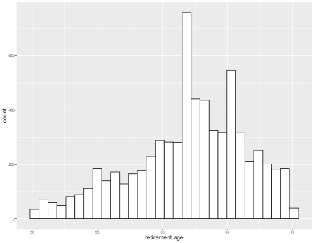
(a) In all samples

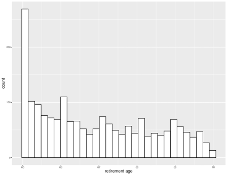
(b) In the treated group

Figure 3: Distribution of retirement age

Using optimal matching as implemented in the optmatch R package (Hansen and Klopfer, 2006), we form $1858$ matched pairs, matching exactly on the year of birth, gender, occupation, and partnered or not, and balance the race, years of education, and smoking status. Table 7 summarizes the covariate balance after matching. After matching, the treated and control groups are well-balanced (Table 7): the standardized differences of all covariates are less than 0.1. Additionally, the propensity score in the treated and control group have good overlap before and after matching (see the Supplementary Materials).

Table 7: Covariate balance after matching.

	Control	Treated	std.diff
Year of birth	1936.27	1936.27	0.00
Female	0.53	0.53	0.00
Non-hispanic white	0.77	0.75	-0.04
Education (yrs)	12.52	12.53	0.00
Occupation: cleaning, building, food prep, and personal services	0.10	0.10	0.00
Occupation: executives and managers	0.16	0.16	0.00
Occupation: production construction and operation occupations	0.28	0.28	0.00
Occupation: professional specialty	0.19	0.19	0.00
Occupation: protection services and armed forces	0.02	0.02	0.00
Occupation: sales and admin	0.25	0.25	0.00
Partnered	0.74	0.74	0.00
Smoke ever	0.63	0.59	-0.08

We considered two potential effect modifiers, namely gender and occupation. More complicated treatment rules can in principle be considered within our framework, though having more treatment rules generally reduces the power of multiple testing. We grouped the $6$ occupations into $2$ broad categories: white collar jobs (executives and managers and professional specialties) and blue collar jobs (sales, administration, protection services, personal services, production, construction, and operation). There were $4$ subgroups defined by these two potential effect modifiers: male, white-collar workers ($G_{1}$), female, white-collar workers ($G_{2}$), male, blue-collar workers ($G_{3}$), and female, blue-collar workers ($G_{4}$). Thus, there were a total of $2^{4}=16$ different regimes formed out of these two effect modifiers. We gave decimal as well as binary codings to the $16$ groups: $r_{0}$ ($r_{0000}$) assigns control to everyone, $r_{8}\,(r_{1000}),r_{4}\,(r_{0100}),r_{2}\,(r_{0010}),r_{1}\,(r_{0001})$ assign treatment to one of the $4$ subgroups, and so forth. We split the matched samples and used $1/4$ of them to plan the test in the other $3/4$. Then we followed the procedures proposed in Section 3 to rank and select the treatment rules.

Figure 4 reports the estimated Hasse diagram at $\Gamma=1.2$; additional results can be found in the Supplementary Materials. The estimated maximal rules for various choices of $\Gamma$ and $\delta$ are reported in Table 8 and the estimated positive rules are reported in the Supplementary Materials. According to Table 8, the maximal rules under the no unmeasured confounding assumption are $r_{11}\,(r_{1011})$ which assigns late retirement to all but female, white-collar workers, $r_{13}\,(r_{1101})$ which assigns late retirement to all but male, blue-collar workers, and $r_{15}\,(r_{1111})$ which assigns treatment to everyone. When $\Gamma$ increases to $1.2$, $r_{9}\,(r_{1001})$ which assigns treatment to male, white-collar workers and female, blue-collar workers, further enters the set of maximal rules. The estimated positive rules suggest that $r_{9}\,(r_{1001})$ and $r_{1}\,(r_{0001})$ which only assigns late retirement to female blue collar workers, though not among the maximal rules at $\Gamma=1$ in Table 8, are the most robust to unmeasured confounding. This suggests that later retirement perhaps benefit female blue-collar workers more than others.

Figure 4: The effect of late retirement on health: Hasse diagram at $\Gamma=1.2$

Table 8: The effect of late retirement on health: $\hat{\mathcal{R}}_{\text{max},\Gamma}$ for different choices of $\Gamma$.

$\Gamma$	$\hat{\mathcal{R}}_{\text{max},\Gamma}$
1.0	$\{r_{11},r_{13},r_{15}\}$
1.2	$\{r_{9},r_{11},r_{13},r_{15}\}$
1.35	$\{r_{1},r_{3},r_{5},r_{7},r_{9},r_{11},r_{13},r_{15}\}$

Does $\Gamma=1.2$ represent a weak or strong unmeasured confounder? Rosenbaum and Silber (2009) proposed to amplify $\Gamma$ to a two-dimensional curve indexed by $(\Lambda,\Delta)$, where $\Lambda$ describes the relationship between the unmeasured confounder and the treatment assignment, and $\Delta$ describes the relationship between the unmeasured confounder and the outcome. For instance, $\Gamma=1.2$ corresponds to an unmeasured confounder associated with a doubling of the odds of late retirement and a $75\%$ increase in the odds of better health status at the age of $70$ in each matched pair, i.e., $(\Delta,\Lambda)=(2.0,1.75)$. Hsu and Small (2013) further proposed to calibrate $(\Lambda,\Delta)$ values to coefficients of observed covariates, however, their method only works for binary outcome and binary treatment. In the Supplementary Materials, we describe a calibration analysis that handle the ordinal self-reported health status level in our application that has $5$ levels.

We follow Hsu and Small (2013) and use a plot to summarize the calibration analysis. In Figure 5, the blue curve represents Rosenbaum and Silber (2009)’s two-dimensional amplification of $\Gamma=1.2$ indexed by $(\Lambda,\Delta)$. The estimated coefficients of observed covariates are represented by black dots (after taking an exponential so they are comparable to $(\Lambda,\Delta)$). We followed the suggestion in Gelman (2008) and standardized all the non-binary covariates to have mean $0$ and standard deviation $0.5$, so the coefficient of each binary variable can be interpreted directly and the coefficients of each continuous/ordinal variable can be interpreted as the effect of a 2-SD increase in the covariate value, which roughly corresponds to flipping a binary variable from $0$ to $1$. Note that all coefficients are under the $\Gamma=1.2$ curve. In fact, $\Gamma=1.2$ roughly corresponds to a moderately strong binary unobserved covariate whose effects on late retirement and health status are comparable to a binary covariate $U$ constructed from smoking and education (red star in Figure 5).

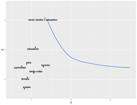
Figure 5: The effect of latent retirement on health: Calibration of the sensitivity analysis. The blue curve is Rosenbaum and Silber (2009)’s amplification of $\Gamma=1.2$. Black dots represent estimated coefficient of each observed covariate. Red marker represents the aggregate effect of flipping smoking status and increasing education by 2 standard deviations.

6 Discussion

In this paper we proposed a general framework to compare, select, and rank treatment rules when there is a limited degree of unmeasured confounding and illustrated the proposed methods by two real data examples. A central message is that the best treatment rule (with the largest estimated value) assuming no unmeasured confounding is often not the most robust to unmeasured confounding. This may have important policy implications when individualized treatment rules are learned from observational data.

Because the value function only defines a partial order on the treatment rules when there is unmeasured confounding, there is a multitude of statistical questions one can ask about selecting and ranking the treatment rules. We have considered three questions that we believe are most relevant to policy research, but there are many other questions (such as in Gibbons et al. (1999)) one could ask.

In principle, our framework can be used with an arbitrary number of prespecified individualized treatment rules. However, to maintain a good statistical power in the multiple testing, the prespecified treatment rules should not be too many. This limitation makes our method most suitable as a confirmatory analysis to complement machine learning algorithms for individualized treatment rule discovery. Alternatively, if the number of decision variables is relatively low due to economic or practical reasons, our method is also reasonably powered for treatment rule discovery.

Appendix A Appendix: Proof of Equation 3

To simplify the notation, suppose $r_{1}(\bm{X}_{i})<r_{2}(\bm{X}_{i})$ for all $1\leq i\leq I$. Let

$$D_{i,\Gamma}=D_{i}-\left(\frac{\Gamma-1}{\Gamma+1}\right)|D_{i,\Gamma}|,\quad\overline{D}=\frac{1}{I}\sum_{i=1}^{I}D_{i},\quad\overline{|D|}=\frac{1}{I}\sum_{i=1}^{I}|D_{i}|,$$

$$\overline{D}_{\Gamma}=(1/I)\sum_{i=1}^{I}D_{i,\Gamma}=\overline{D}-\left(\frac{\Gamma-1}{\Gamma+1}\right)\overline{|D|},$$

and

$$se(\overline{D}_{\Gamma})^{2}=\frac{1}{I^{2}}\sum_{i=1}^{I}(D_{i,\Gamma}-\overline{D}_{\Gamma})^{2}.$$

When $\mathbb{E}[D_{i}]>0$, $\Gamma^{\ast}(r_{1},r_{2})$ is obtained by solving the equation below in $\Gamma$:

$$\frac{\overline{D}_{\Gamma}}{se(\overline{D}_{\Gamma})}=\Phi^{-1}(1-\alpha).$$ (5)

Square both sides of the equation above and plug in the expressions for $\overline{D}_{\Gamma}$ and $se(\overline{D}_{\Gamma})^{2}$. Let $\kappa=(\Gamma-1)/(\Gamma+1)$ and $z_{\alpha}=\Phi^{-1}(1-\alpha)$. Denote

$$z_{\alpha}=\Phi^{-1}(1-\alpha),\quad\overline{|D|}=\frac{1}{I}\sum_{i=1}^{I}|D_{i}|,\quad,$$

and

$$s^{2}_{D}=\frac{1}{I}\sum_{i=1}^{I}(D_{i}-\overline{D})^{2},\quad s^{2}_{|D|}=\frac{1}{I}\sum_{i=1}^{I}(|D_{i}|-\overline{|D|})^{2},\quad s_{D,|D|}=\frac{1}{I}\sum_{i=1}^{I}(D_{i}-\overline{D})(|D_{i}|-\overline{|D|}).$$

One can show the sensitivity value $\Gamma^{\ast}(r_{1},r_{2})$ corresponds to $\kappa^{\ast}$ that solves the following quadratic equation:

$$\left(\overline{|D|}^{2}-\frac{1}{I}s^{2}_{|D|}z_{\alpha}^{2}\right)\kappa^{2}-2\left(\overline{D}\overline{|D|}-\frac{1}{I}s_{D,|D|}z_{\alpha}^{2}\right)\kappa+\overline{D}^{2}-\frac{1}{I}s^{2}_{D}c^{2}_{\alpha}=0.$$

Specifically, we have

$$\kappa^{\ast}=\frac{{\overline{D}\overline{|D|}-\frac{1}{I}s_{D,|D|}z_{\alpha}^{2}}\pm\sqrt{\Delta}}{\overline{|D|}^{2}-\frac{1}{I}s^{2}_{|D|}z_{\alpha}^{2}},$$ (6)

where $\Delta=(\overline{D}\overline{|D|}-\frac{1}{I}s_{D,|D|}z_{\alpha}^{2})^{2}-(\overline{|D|}^{2}-\frac{1}{I}s^{2}_{|D|}z_{\alpha}^{2})(\overline{D}^{2}-\frac{1}{I}s^{2}_{D}c^{2}_{\alpha})$.

Note

$$\sqrt{\Delta}=z_{\alpha}\sqrt{\frac{1}{I}\left(s^{2}_{|D|}\cdot\overline{D}^{2}+s^{2}_{D}\cdot\overline{|D|}^{2}-2\overline{D}\overline{|D|}s_{D,|D|}\right)+\frac{1}{I^{2}}z_{\alpha}^{2}\left(s_{D,|D|}^{2}-s^{2}_{|D|}\cdot s^{2}_{D}\right)}.$$

Let us denote $A=\mathbb{E}[D]\cdot\mathbb{E}[|D|]$, $B=-z_{\alpha}\sqrt{\sigma^{2}_{|D|}\cdot\mathbb{E}[D]^{2}+\sigma^{2}_{D}\cdot\mathbb{E}[|D|]^{2}-2\mathbb{E}[D]\mathbb{E}[|D|]\sigma_{D,|D|}}$, $C=\mathbb{E}[|D|]^{2}$, $R_{1}=\sqrt{I}(\overline{D}\overline{|D|}-A)$, $R_{2}=\sqrt{I}(\overline{|D|}^{2}-C)$.

We have

$$\kappa^{\ast}=\frac{A+\frac{1}{\sqrt{I}}R_{1}+\frac{1}{\sqrt{I}}B}{C+\frac{1}{\sqrt{I}}R_{2}}+o_{p}\left(\frac{1}{\sqrt{I}}\right)=\frac{(A+\frac{1}{\sqrt{I}}R_{1}+\frac{1}{\sqrt{I}}B)\cdot(1-\frac{1}{\sqrt{I}}\frac{R_{2}}{C})}{C}+o_{p}\left(\frac{1}{\sqrt{I}}\right).$$

Scale both sides by $\sqrt{I}$ and rearrange the terms, we have

$$\sqrt{I}\left(\kappa^{\ast}-\frac{A}{C}\right)=\frac{B}{C}+\frac{1}{C}R_{1}-\frac{A}{C^{2}}R_{2}+o_{p}(1).$$

Moreover, let $\phi\mathrel{\mathop{\mathchar 58\relax}}\mathbb{R}^{2}\mapsto\mathbb{R}^{2}=(xy,y^{2})$:

$$\sqrt{I}\begin{pmatrix}\overline{D}-\mathbb{E}[D]\\ \overline{|D|}-\mathbb{E}[|D|]\end{pmatrix}\sim N(0,\Sigma),\quad\text{implies}\quad\begin{pmatrix}R_{1}\\ R_{2}\end{pmatrix}=\sqrt{I}\begin{pmatrix}\overline{D}\overline{|D|}-\mathbb{E}[D]\cdot\mathbb{E}[|D|]\\ \overline{|D|}^{2}-\mathbb{E}[|D|]^{2}\end{pmatrix}\sim N(0,\phi^{\prime}\Sigma(\phi^{\prime})^{T}),$$

where $\Sigma=\begin{pmatrix}\text{Var}[D],&\text{Cov}(D,|D|)\\ \text{Cov}(D,|D|),&\text{Var}[|D|]\end{pmatrix}$ and $\phi^{\prime}=\begin{pmatrix}\mathbb{E}[|D|],&\mathbb{E}[D]\\ 0,&2\mathbb{E}[|D|]\end{pmatrix}$.

Plug in the expressions for $A$, $B$, and $C$ and compute the variance-covariance matrix of $(1/C,-A/C^{2})(R_{1},R_{2})^{T}$:

$$\sqrt{I}\left(\kappa^{\ast}-\frac{\mathbb{E}[D]}{\mathbb{E}[|D|]}\right)\sim N(z_{\alpha}\mu,\leavevmode\nobreak\ \sigma^{2})$$

where

$$\mu=-\frac{\sqrt{\sigma^{2}_{|D|}\cdot\mathbb{E}[D]^{2}+\sigma^{2}_{D}\cdot\mathbb{E}[|D|]^{2}-2\mathbb{E}[D]\mathbb{E}[|D|]\sigma_{D,|D|}}}{\mathbb{E}[|D|]^{2}},$$

and

$$\sigma^{2}=\frac{\text{Var}[D]\mathbb{E}^{2}[|D|]-\text{Var}[|D|]\mathbb{E}^{2}[D]-2\mathbb{E}[D]\mathbb{E}[|D|]\text{Cov}(D,|D|)+2\mathbb{E}^{2}[D]\text{Var}[|D|]}{\mathbb{E}^{4}[|D|]}.$$

The Supplementary Materials contain additional appendices about matching in observational studies and further simulation and real data results.

References

- Alavinia and Burdorf [2008] Seyed Mohammad Alavinia and Alex Burdorf. Unemployment and retirement and ill-health: a cross-sectional analysis across european countries. International Archives of Occupational and Environmental Health, 82(1):39–45, 2008.
- Athey and Wager [2017] Susan Athey and Stefan Wager. Efficient policy learning. arXiv preprint arXiv:1702.02896, 2017.
- Börsch-Supan and Jürges [2006] Axel Börsch-Supan and Hendrik Jürges. Early retirement, social security and well-being in germany. Technical report, National Bureau of Economic Research, 2006.
- Calvo et al. [2012] Esteban Calvo, Natalia Sarkisian, and Christopher R. Tamborini. Causal Effects of Retirement Timing on Subjective Physical and Emotional Health. The Journals of Gerontology: Series B, 68(1):73–84, 11 2012. ISSN 1079-5014. doi: 10.1093/geronb/gbs097. URL https://doi.org/10.1093/geronb/gbs097.
- Cornfield et al. [1959] J. Cornfield, W. Haenszel, E. Hammond, A. Lilienfeld, M. Shimkin, and E. Wynder. Smoking and lung cancer. Journal of the National Cancer Institute, 22:173–203, 1959.
- Dave et al. [2008] Dhaval Dave, Inas Rashad, and Jasmina Spasojevic. The effects of retirement on physical and mental health outcomes. Southern Economic Journal, 75(2):497–523, 2008. ISSN 00384038. URL http://www.jstor.org/stable/27751397.
- Dudík et al. [2014] Miroslav Dudík, Dumitru Erhan, John Langford, Lihong Li, et al. Doubly robust policy evaluation and optimization. Statistical Science, 29(4):485–511, 2014.
- Fogarty [2016] Colin B Fogarty. Studentized sensitivity analysis for the sample average treatment effect in paired observational studies. arXiv preprint arXiv:1609.02112, 2016.
- Gelman [2008] A. Gelman. Scaling regression inputs by dividing by two standard deviations. Statistics in Medicine, 27:2865–2873, 2008.
- Gibbons et al. [1999] Jean Dickinson Gibbons, Ingram Olkin, and Milton Sobel. Selecting and ordering populations: A new statistical methodology. SIAM, 2nd edition, 1999.
- Gupta and Panchapakesan [1979] Shanti S Gupta and Subramanian Panchapakesan. Multiple decision procedures: Theory and methodology of selecting and ranking populations. SIAM, 1979.
- Hansen and Klopfer [2006] Ben B. Hansen and Stephanie Olsen Klopfer. Optimal full matching and related designs via network flows. Journal of Computational and Graphical Statistics, 15(3):609–627, 2006.
- Heller et al. [2009] Ruth Heller, Paul R Rosenbaum, and Dylan S Small. Split samples and design sensitivity in observational studies. Journal of the American Statistical Association, 104(487):1090–1101, 2009.
- Hsu and Small [2013] J. Y. Hsu and D. S. Small. Calibrating sensitivity analyses to observed covariates in observational studies. Biometrics, 69:803–811, 2013.
- Hsu et al. [2013] Jesse Y. Hsu, Dylan S. Small, and Paul R. Rosenbaum. Effect modification and design sensitivity in observational studies. Journal of the American Statistical Association, 108(501):135–148, 2013. doi: 10.1080/01621459.2012.742018. URL https://doi.org/10.1080/01621459.2012.742018.
- Kallus [2017] Nathan Kallus. Recursive partitioning for personalization using observational data. In Proceedings of the 34th International Conference on Machine Learning-Volume 70, pages 1789–1798. JMLR. org, 2017.
- Kallus and Zhou [2018] Nathan Kallus and Angela Zhou. Confounding-robust policy improvement. In Advances in Neural Information Processing Systems, pages 9269–9279, 2018.
- Kallus et al. [2018] Nathan Kallus, Xiaojie Mao, and Angela Zhou. Interval estimation of individual-level causal effects under unobserved confounding. arXiv preprint arXiv:1810.02894, 2018.
- Koch and Gansky [1996] Gary G Koch and Stuart A Gansky. Statistical considerations for multiplicity in confirmatory protocols. Drug Information Journal, 30(2):523–534, 1996.
- Kosorok and Laber [2019] Michael R. Kosorok and Eric B. Laber. Precision medicine. Annual Review of Statistics and Its Application, 6(1):263–286, 2019. doi: 10.1146/annurev-statistics-030718-105251. URL https://doi.org/10.1146/annurev-statistics-030718-105251.
- Moodie et al. [2012] Erica EM Moodie, Bibhas Chakraborty, and Michael S Kramer. Q-learning for estimating optimal dynamic treatment rules from observational data. Canadian Journal of Statistics, 40(4):629–645, 2012.
- Morrow-Howell et al. [2001] Nancy Morrow-Howell, James Hinterlong, Michael Sherraden, et al. Productive aging: Concepts and challenges. JHU Press, 2001.
- Murphy [2003] Susan A Murphy. Optimal dynamic treatment regimes. Journal of the Royal Statistical Society: Series B (Statistical Methodology), 65(2):331–355, 2003.
- Qian and Murphy [2011] Min Qian and Susan A. Murphy. Performance guarantees for individualized treatment rules. The Annals of Statistics, 39(2):1180–1210, 2011. ISSN 00905364. URL http://www.jstor.org/stable/29783670.
- RAND [2018] RAND. RAND HRS Longitudinal File 2014 (V2) public use dataset. Produced by the RAND Center for the Study of Aging, with funding from the National Institute on Aging and the Social Security Administration. 2018.
- Robins [2004] James M Robins. Optimal structural nested models for optimal sequential decisions. In Proceedings of the second seattle Symposium in Biostatistics, pages 189–326. Springer, 2004.
- Rosenbaum [1987] P. R. Rosenbaum. Sensitivity analysis for certain permutation inferences in matched observational studies. Biometrika, 74:13–26, 1987.
- Rosenbaum [2002] P. R. Rosenbaum. Observational Studies. Springer., 2002.
- Rosenbaum [2015] P. R. Rosenbaum. Bahadur Efficiency of Sensitivity Analyses in Observational Studies. Journal of the American Statistical Association, 110:205–217, 2015.
- Rosenbaum and Silber [2009] P. R. Rosenbaum and J. H. Silber. Amplification of sensitivity analysis in matched observational studies. Journal of the American Statistical Association, 104:1398–1405, 2009.
- Rosenbaum [2004] Paul R Rosenbaum. Design sensitivity in observational studies. Biometrika, 91(1):153–164, 2004.
- Rosenbaum [2011] Paul R Rosenbaum. A new U-statistic with superior design sensitivity in matched observational studies. Biometrics, 67(3):1017–1027, 2011.
- Sonnega et al. [2014] Amanda Sonnega, Jessica D Faul, Mary Beth Ofstedal, Kenneth M Langa, John WR Phillips, and David R Weir. Cohort Profile: the Health and Retirement Study (HRS). International Journal of Epidemiology, 43(2):576–585, 03 2014. ISSN 0300-5771. doi: 10.1093/ije/dyu067. URL https://doi.org/10.1093/ije/dyu067.
- Tan [2006] Zhiqiang Tan. A distributional approach for causal inference using propensity scores. Journal of the American Statistical Association, 101(476):1619–1637, 2006.
- Westerlund et al. [2009] Hugo Westerlund, Mika Kivimäki, Archana Singh-Manoux, Maria Melchior, Jane E Ferrie, Jaana Pentti, Markus Jokela, Constanze Leineweber, Marcel Goldberg, Marie Zins, and Jussi Vahtera. Self-rated health before and after retirement in france (gazel): a cohort study. The Lancet, 374(9705):1889 – 1896, 2009. ISSN 0140-6736. doi: https://doi.org/10.1016/S0140-6736(09)61570-1. URL http://www.sciencedirect.com/science/article/pii/S0140673609615701.
- Westfall and Krishen [2001] Peter H Westfall and Alok Krishen. Optimally weighted, fixed sequence and gatekeeper multiple testing procedures. Journal of Statistical Planning and Inference, 99(1):25–40, 2001.
- Wu et al. [2019] Peng Wu, Donglin Zeng, and Yuanjia Wang. Matched learning for optimizing individualized treatment strategies using electronic health records. Journal of the American Statistical Association, 0(0):1–23, 2019. doi: 10.1080/01621459.2018.1549050. URL https://doi.org/10.1080/01621459.2018.1549050.
- Yadlowsky et al. [2018] Steve Yadlowsky, Hongseok Namkoong, Sanjay Basu, John Duchi, and Lu Tian. Bounds on the conditional and average treatment effect in the presence of unobserved confounders. arXiv preprint arXiv:1808.09521, 2018.
- Zhang et al. [2018] Yichi Zhang, Eric B Laber, Marie Davidian, and Anastasios A Tsiatis. Interpretable dynamic treatment regimes. Journal of the American Statistical Association, 113(524):1541–1549, 2018.
- Zhao [2018] Qingyuan Zhao. On sensitivity value of pair-matched observational studies. Journal of the American Statistical Association, 0(0):1–10, 2018. doi: 10.1080/01621459.2018.1429277. URL https://doi.org/10.1080/01621459.2018.1429277.
- Zhao et al. [2018] Qingyuan Zhao, Dylan S Small, and Paul R Rosenbaum. Cross-screening in observational studies that test many hypotheses. Journal of the American Statistical Association, 113(523):1070–1084, 2018.
- Zhao et al. [2019a] Qingyuan Zhao, Dylan S. Small, and Bhaswar B. Bhattacharya. Sensitivity analysis for inverse probability weighting estimators via the percentile bootstrap, 2019a.
- Zhao et al. [2019b] Ying-Qi Zhao, Eric B Laber, Yang Ning, Sumona Saha, and Bruce Sands. Efficient augmentation and relaxation learning for individualized treatment rules using observational data. Journal of Machine Learning Research, 20:1–23, 2019b.
- Zhao et al. [2012] Yingqi Zhao, Donglin Zeng, A. John Rush, and Michael R. Kosorok. Estimating individualized treatment rules using outcome weighted learning. Journal of the American Statistical Association, 107(499):1106–1118, 2012. doi: 10.1080/01621459.2012.695674. URL https://doi.org/10.1080/01621459.2012.695674. PMID: 23630406.