Lagrangian Decomposition for Neural Network Verification

Abstract

A fundamental component of neural network verification is the computation of bounds on the values their outputs can take. Previous methods have either used off-the-shelf solvers, discarding the problem structure, or relaxed the problem even further, making the bounds unnecessarily loose. We propose a novel approach based on Lagrangian Decomposition. Our formulation admits an efficient supergradient ascent algorithm, as well as an improved proximal algorithm. Both the algorithms offer three advantages: (i) they yield bounds that are provably at least as tight as previous dual algorithms relying on Lagrangian relaxations; (ii) they are based on operations analogous to forward/backward pass of neural networks layers and are therefore easily parallelizable, amenable to GPU implementation and able to take advantage of the convolutional structure of problems; and (iii) they allow for anytime stopping while still providing valid bounds. Empirically, we show that we obtain bounds comparable with off-the-shelf solvers in a fraction of their running time, and obtain tighter bounds in the same time as previous dual algorithms. This results in an overall speed-up when employing the bounds for formal verification. Code for our algorithms is available at https://github.com/oval-group/decomposition-plnn-bounds.

1 INTRODUCTION

As deep learning powered systems become more and more common, the lack of robustness of neural networks and their reputation for being “Black Boxes” is increasingly worrisome. In order to deploy them in critical scenarios where safety and robustness would be a prerequisite, we need to invent techniques that can prove formal guarantees for neural network behaviour. A particularly desirable property is resistance to adversarial examples (Goodfellow et al.,, 2015, Szegedy et al.,, 2014): perturbations maliciously crafted with the intent of fooling even extremely well performing models. After several defenses were proposed and subsequently broken (Athalye et al.,, 2018, Uesato et al.,, 2018), some progress has been made in being able to formally verify whether there exist any adversarial examples in the neighbourhood of a data point (Tjeng et al.,, 2019, Wong and Kolter,, 2018).

Verification algorithms fall into three categories: unsound (some false properties are proven false), incomplete (some true properties are proven true), and complete (all properties are correctly verified as either true or false). A critical component of the verification systems developed so far is the computation of lower and upper bounds on the output of neural networks when their inputs are constrained to lie in a bounded set. In incomplete verification, by deriving bounds on the changes of the prediction vector under restricted perturbations, it is possible to identify safe regions of the input space. These results allow the rigorous comparison of adversarial defenses and prevent making overconfident statements about their efficacy (Wong and Kolter,, 2018). In complete verification, bounds can also be used as essential subroutines of Branch and Bound complete verifiers (Bunel et al.,, 2018). Finally, bounds might also be used as a training signal to guide the network towards greater robustness and more verifiability (Gowal et al.,, 2018, Mirman et al.,, 2018, Wong and Kolter,, 2018).

Most previous algorithms for computing bounds are either computationally expensive (Ehlers,, 2017) or sacrifice a lot of tightness in order to scale (Gowal et al.,, 2018, Mirman et al.,, 2018, Wong and Kolter,, 2018). In this work, we design novel customised relaxations and their corresponding solvers for obtaining bounds on neural networks. Our approach offers the following advantages:

• While previous approaches to neural network bounds (Dvijotham et al.,, 2018) are based on Lagrangian relaxations, we derive a new family of optimization problems for neural network bounds through Lagrangian Decomposition, which in general yields duals at least as strong as those obtained through Lagrangian relaxation (Guignard and Kim,, 1987). We in fact prove that, in the context of ReLU networks, for any dual solution from the approach by Dvijotham et al., (2018), the bounds output by our dual are as least as tight. We demonstrate empirically that this derivation computes tighter bounds in the same time when using supergradient methods. We further improve on the performance by devising a proximal solver for the problem, which decomposes the task into a series of strongly convex subproblems. For each, we use an iterative method for which we derive optimal step sizes.

• Both the supergradient and the proximal method operate through linear operations similar to those used during network forward/backward passes. As a consequence, we can leverage the convolutional structure when necessary, while standard solvers are often restricted to treating it as a general linear operation. Moreover, both methods are easily parallelizable: when computing bounds on the activations at layer $k$, we need two solve two problems for each hidden unit of the network (for the upper and lower bounds). These can all be solved in parallel. In complete verification, we need to compute bounds for several different problem domains at once: we solve these problems in parallel as well. Our GPU implementation thus allows us to solve several hundreds of linear programs at once on a single GPU, a level of parallelism that would be hard to match on CPU-based systems.

• Most standard linear programming based relaxations (Ehlers,, 2017) will only return a valid bound if the problem is solved to optimality. Others, like the dual simplex method employed by off-the-shelf solvers (Gurobi Optimization,, 2020) have a very high cost per iteration and will not yield tight bounds without incurring significant computational costs. Both methods described in this paper are anytime (terminating it before convergence still provides a valid bound), and can be interrupted at very small granularity. This is useful in the context of a subroutine for complete verifiers, as this enables the user to choose an appropriate speed versus accuracy trade-off. It also offers great versatility as an incomplete verification method.

2 RELATED WORKS

Bound computations are mainly used for formal verification methods. Some methods are complete (Cheng et al.,, 2017, Ehlers,, 2017, Katz et al.,, 2017, Tjeng et al.,, 2019, Xiang et al.,, 2017), always returning a verdict for each problem instances. Others are incomplete, based on relaxations of the verification problem. They trade speed for completeness: while they cannot verify properties for all problem instances, they scale significantly better. Two main types of bounds have been proposed: on the one hand, some approaches (Ehlers,, 2017, Salman et al.,, 2019) rely on off-the-shelf solvers to solve accurate relaxations such as PLANET (Ehlers,, 2017), which is the best known linear-sized approximation of the problem. On the other hand, as PLANET and other more complex relaxations do not have closed form solutions, some researchers have also proposed easier to solve, looser formulations (Gowal et al.,, 2018, Mirman et al.,, 2018, Weng et al.,, 2018, Wong and Kolter,, 2018). Explicitly or implicitly, these are all equivalent to propagating a convex domain through the network to overapproximate the set of reachable values. Our approach consists in tackling a relaxation equivalent to the PLANET one (although generalised beyond ReLU), by designing a custom solver that achieves faster performance without sacrificing tightness. Some potentially tighter convex relaxations exist but involve a quadratic number of variables, such as the semi-definite programming method of Raghunathan et al., (2018) . Better relaxations obtained from relaxing strong Mixed Integer Programming formulations (Anderson et al.,, 2019) have a quadratic number of variables or a potentially exponential number of constraints. We do not address them here.

A closely related approach to ours is the work of Dvijotham et al., (2018). Both their method and ours are anytime and operate on similar duals. While their dual is based on the Lagrangian relaxation of the non-convex problem, ours is based on the Lagrangian Decomposition of the nonlinear activation’s convex relaxation. Thanks to the properties of Lagrangian Decomposition (Guignard and Kim,, 1987), we can show that our dual problem provides better bounds when evaluated on the same dual variables. The relationship between the two duals is studied in detail in section 4.2. Moreover, in terms of the followed optimization strategy, in addition to using a supergradient method like Dvijotham et al., (2018), we present a proximal method, for which we can derive optimal step sizes. We show that these modifications enable us to compute tighter bounds using the same amount of compute time.

3 PRELIMINARIES

Throughout this paper, we will use bold lower case letters (like $\mathbf{z}$) to represent vectors and upper case letters (like $W$) to represent matrices. Brackets are used to indicate the $i$-th coordinate of a vector ($\mathbf{z}[i]$), and integer ranges (e.g., $[1,n-1]$). We will study the computation of the lower bound problem based on a feedforward neural network, with element-wise activation function $\sigma\left(\cdot\right)$. The network inputs are restricted to a convex domain $\mathcal{C}$, over which we assume that we can easily optimise linear functions. This is the same assumption that was made by Dvijotham et al., (2018). The computation for an upper bound is analogous. Formally, we wish to solve the following problem:

$$\smash{\min_{\mathbf{z},\mathbf{\hat{z}}}}\quad \mathbf{\hat{z}}_{n}$$ (1a)

s.t. $$\mathbf{z}_{0}\in\mathcal{C},$$ (1b)

$$\mathbf{\hat{z}}_{k+1}=W_{k+1}\mathbf{z}_{k}+\mathbf{b}_{k+1}\quad k\in\left[1,n-1\right],$$ (1c)

$$\mathbf{z}_{k}=\sigma\left(\mathbf{\hat{z}}_{k}\right)\quad k\in\left[1,n-1\right].$$ (1d)

The output of the $k$-th layer of the network before and after the application of the activation function are denoted by $\mathbf{\hat{z}}_{k}$ and $\mathbf{z}_{k}$ respectively. Constraints (1c) implements the linear layers (fully connected or convolutional) while constraints (1d) implement the non-linear activation function. Constraints (1b) define the region over which the bounds are being computed. While our method can be extended to more complex networks (such as ResNets), we focus on problem (1) for the sake of clarity.

The difficulty of problem (1) comes from the non-linearity (1d). Dvijotham et al., (2018) tackle it by relaxing (1c) and (1b) via Lagrangian multipliers, yielding the following dual:

$$\begin{split}\max_{\bm{\mu},\bm{\lambda}}\enskip&d(\bm{\mu},\bm{\lambda}),\quad\text{where: }\\ d(\bm{\mu},\bm{\lambda})=&\min_{\mathbf{z},\mathbf{\hat{z}}}\quad W_{n}\mathbf{z}_{n-1}+\mathbf{b}_{n}\\ \qquad+&\sum_{k=1}^{n-1}\bm{\mu}_{k}^{T}\left(\mathbf{\hat{z}}_{k}-W_{k}\mathbf{z}_{k-1}-\mathbf{b}_{k}\right)\\ \qquad+&\sum_{k=1}^{n-1}\bm{\lambda}_{k}^{T}\left(\mathbf{z}_{k}-\sigma(\mathbf{\hat{z}}_{k})\right)\\ \text{s.t. }\quad&\mathbf{l}_{k}\leq\mathbf{\hat{z}}_{k}\leq\mathbf{u}_{k}\qquad\qquad k\in\left[1,n-1\right],\\ &\sigma(\mathbf{l}_{k})\leq\mathbf{z}_{k}\leq\sigma(\mathbf{u}_{k})\qquad k\in\left[1,n-1\right],\\ &\mathbf{z}_{0}\in\mathcal{C}.\end{split}$$ (2)

If $\sigma$ is a ReLU, this relaxation is equivalent (Dvijotham et al.,, 2018) to the PLANET relaxation (Ehlers,, 2017). The dual requires upper ($\mathbf{u}_{k}$) and lower bounds ($\mathbf{l}_{k}$) on the value that $\mathbf{\hat{z}}_{k}$ can take, for $k\in\left[0..n-1\right]$. We call these intermediate bounds: we detail how to compute them in appendix B. The dual algorithm by Dvijotham et al., (2018) solves (2) via supergradient ascent.

4 LAGRANGIAN DECOMPOSITION

We will now describe a novel approach to solve problem  (1), and relate it to the dual algorithm by  Dvijotham et al., (2018). We will focus on computing bounds for an output of the last layer of the neural network.

4.1 PROBLEM DERIVATION

Our approach is based on Lagrangian decomposition, also known as variable splitting (Guignard and Kim,, 1987). Due to the compositional structure of neural networks, most constraints involve only a limited number of variables. As a result, we can split the problem into meaningful, easy to solve subproblems. We then impose constraints that the solutions of the subproblems should agree.

We start from the original non-convex primal problem (1), and substitute the nonlinear activation equality (1d) with a constraint corresponding to its convex hull. This leads to the following convex program:

$$\smash{\min_{\mathbf{z},\mathbf{\hat{z}}}}\enskip \mathbf{\hat{z}}_{n}$$ (3a)

s.t. $$\mathbf{z}_{0}\in\mathcal{C},$$ (3b)

$$\mathbf{\hat{z}}_{k+1}=W_{k+1}\mathbf{z}_{k}+\mathbf{b}_{k+1}\enskip k\in\left[1,n-1\right],$$ (3c)

$$\texttt{cvx\_hull}_{\sigma}\left(\mathbf{\hat{z}}_{k},\mathbf{z}_{k},\mathbf{l}_{k},\mathbf{u}_{k}\right)\enskip k\in\left[1,n-1\right].$$ (3d)

In the following, we will use ReLU activation functions as an example, and employ the PLANET relaxation as its convex hull, which is the tightest linearly sized relaxation published thus far. By linearly sized, we mean that the numbers of variables and constraints to describe the relaxation only grow linearly with the number of units in the network. We stress that the derivation can be extended to other non-linearities. For example, appendix A describes the case of sigmoid activation function. For ReLUs, this convex hull takes the following form (Ehlers,, 2017):

$$\texttt{cvx\_hull}_{\sigma}\equiv \text{if }\mathbf{l}_{k}[i]\leq 0;\mathbf{u}_{k}[i]\geq 0:$$

$$\texttt{cvx\_hull}_{\sigma}\equiv \quad\mathbf{z}_{k}[i]\geq 0,\quad\mathbf{z}_{k}[i]\geq\mathbf{\hat{z}}_{k}[i],$$ (4a)

$$\texttt{cvx\_hull}_{\sigma}\equiv \quad\mathbf{z}_{k}[i]\leq\frac{\mathbf{u_{k}}[i](\mathbf{\hat{z}}_{k}[i]-\mathbf{l}_{k}[i])}{\mathbf{u_{k}}[i]-\mathbf{l_{k}}[i]}.$$

$$\texttt{cvx\_hull}_{\sigma}\equiv \text{if }\mathbf{u}_{k}[i]\leq 0:$$

$$\texttt{cvx\_hull}_{\sigma}\equiv \quad\mathbf{z}_{k}[i]=0.$$ (4b)

$$\texttt{cvx\_hull}_{\sigma}\equiv \text{if }\mathbf{l}_{k}[i]\geq 0:$$

$$\texttt{cvx\_hull}_{\sigma}\equiv \quad\mathbf{z}_{k}[i]=\mathbf{\hat{z}}_{k}[i].$$ (4c)

Constraints (4a), (4b), and (4c) corresponds to the relaxation of the ReLU (1d) in different cases (respectively: ambiguous state, always blocking or always passing).

To obtain a decomposition, we divide the constraints into subsets. Each subset will correspond to a pair of an activation layer, and the linear layer coming after it. The only exception is the first linear layer which is combined with the restriction of the input domain to $\mathcal{C}$. This choice is motivated by the fact that for piecewise-linear activation functions, we will be able to easily perform linear optimisation over the resulting subdomains. For a different activation function, it might be required to have a different decomposition. Formally, we introduce the following notation for subsets of constraints:

$$\mathcal{P}_{0}(\mathbf{z}_{0},\mathbf{\hat{z}}_{1})\equiv\begin{cases}\mathbf{z}_{0}\in\mathcal{C}\\ \mathbf{\hat{z}}_{1}=W_{1}\mathbf{z}_{0}+\mathbf{b}_{1},\end{cases}$$ (5)

$$\mathcal{P}_{k}(\mathbf{\hat{z}}_{k},\mathbf{\hat{z}}_{k+1})\equiv\begin{cases}\mathbf{l}_{k}\leq\mathbf{\hat{z}}_{k}\leq\mathbf{u}_{k},\textstyle\hfil\\ \texttt{cvx\_hull}_{\sigma}\left(\mathbf{\hat{z}}_{k},\mathbf{z}_{k},\mathbf{l}_{k},\mathbf{u}_{k}\right),\\ \mathbf{\hat{z}}_{k+1}=W_{k+1}\mathbf{z}_{k}+\mathbf{b}_{k}.\end{cases}$$ (6)

The set $\mathcal{P}_{k}$ is defined without an explicit dependency on $\mathbf{z}_{k}$ because $\mathbf{z}_{k}$ only appears internally to the subset of constraints and is not involved in the objective function. Using this grouping of the constraints, we can concisely write problem (3) as:

$$\begin{split}\smash{\min_{\mathbf{z},\mathbf{\hat{z}}}}&\quad\mathbf{\hat{z}}_{n}\qquad\text{s.t. }\quad\mathcal{P}_{0}(\mathbf{z}_{0},\mathbf{\hat{z}}_{1}),\\ &\mathcal{P}_{k}(\mathbf{\hat{z}}_{k},\mathbf{\hat{z}}_{k+1})\qquad k\in\left[1,n-1\right].\end{split}$$ (7)

To obtain a Lagrangian decomposition, we duplicate the variables so that each subset of constraints has its own copy of the variables it is involved in. Formally, we rewrite problem (7) as follows:

$$\smash{\min_{\mathbf{z},\mathbf{\hat{z}}}} \quad\mathbf{\hat{z}}_{A,n}$$ (8a)

s.t. $$\quad\mathcal{P}_{0}(\mathbf{z}_{0},\mathbf{\hat{z}}_{A,1}),$$ (8b)

$$\quad\mathcal{P}_{k}(\mathbf{\hat{z}}_{B,k},\mathbf{\hat{z}}_{A,k+1}) \qquad k\in\left[1,n-1\right],$$ (8c)

$$\quad\mathbf{\hat{z}}_{A,k}=\mathbf{\hat{z}}_{B,k} \qquad k\in\left[1,n-1\right].$$ (8d)

The additional equality constraints (8d) impose agreements between the various copies of variables. We introduce the dual variables $\bm{\rho}$ and derive the Lagrangian dual:

$$\begin{split}\max_{\bm{\rho}}\enskip&q(\bm{\rho}),\quad\text{where: }\\[-4.0pt] q\left(\bm{\rho}\right)&=\min_{\mathbf{z},\mathbf{\hat{z}}}\ \mathbf{\hat{z}}_{A,n}+\sum_{k=1}^{n-1}\bm{\rho}_{k}^{T}\left(\mathbf{\hat{z}}_{B,k}-\mathbf{\hat{z}}_{A,k}\right)\\[5.0pt] \text{s.t. }\quad&\mathcal{P}_{0}(\mathbf{z}_{0},\mathbf{\hat{z}}_{A,1}),\\ &\mathcal{P}_{k}(\mathbf{\hat{z}}_{B,k},\mathbf{\hat{z}}_{A,k+1})\qquad k\in\left[1,n-1\right].\end{split}$$ (9)

Any value of $\bm{\rho}$ provides a valid lower bound by virtue of weak duality. While we will maximise over the choice of dual variables in order to obtain as tight a bound as possible, we will be able to interrupt the optimisation process at any point and obtain a valid bound by evaluating $q$.

We stress that, at convergence, problems (9) and (2) will yield the same bounds, as they are both reformulations of the same convex problem. This does not imply that the two derivations yield solvers with the same efficiency. In fact, we will next prove that, for ReLU-based networks, problem (9) yields bounds at least as tight as a corresponding dual solution from problem (2).

4.2 DUALS COMPARISON

We now compare our dual problem (9) with problem (2) by Dvijotham et al., (2018). From the high level perspective, our decomposition considers larger subsets of constraints and hence results in a smaller number of variables to optimize. We formally prove that, for ReLU-based neural networks, our formulation dominates theirs, producing tighter bounds based on the same dual variables.

Theorem 1.

Let us assume $\sigma(\mathbf{\hat{z}}_{k})=\max(\mathbf{0},\mathbf{\hat{z}}_{k})$. For any solution $\bm{\mu},\bm{\lambda}$ of dual (2) by Dvijotham et al., (2018) yielding bound $d(\bm{\mu},\bm{\lambda})$, it holds that $q(\bm{\mu})\geq d(\bm{\mu},\bm{\lambda})$.

Proof.

See appendix E. ∎

Our dual is also related to the one that Wong and Kolter, (2018) operates in. We show in appendix F how our problem can be initialised to a set of dual variables so as to generate a bound matching the one provided by their algorithm. We use this approach as our initialisation for incomplete verification ($\S$ 6.3).

5 SOLVERS FOR LAGRANGIAN DECOMPOSITION

Now that we motivated the use of dual (9) over problem (2), it remains to show how to solve it efficiently in practice. We present two methods: one based on supergradient ascent, the other on proximal maximisation. A summary, including pseudo-code, can be found in appendix D.

5.1 SUPERGRADIENT METHOD

As Dvijotham et al., (2018) use supergradient methods on their dual, we start by applying it on problem (9) as well.

At a given point $\bm{\rho}$, obtaining the supergradient requires us to know the values of $\mathbf{\hat{z}}_{A}$ and $\mathbf{\hat{z}}_{B}$ for which the inner minimisation is achieved. Based on the identified values of $\mathbf{\hat{z}}_{A}^{*}$ and $\mathbf{\hat{z}}_{B}^{*}$, we can then compute the supergradient $\nabla_{\bm{\rho}}q=\mathbf{\hat{z}}_{B}^{*}-\mathbf{\hat{z}}_{A}^{*}$. The updates to $\bm{\rho}$ are then the usual supergradient ascent updates:

$$\bm{\rho}^{t+1}=\bm{\rho}^{t}+\alpha^{t}\nabla_{\bm{\rho}}q(\bm{\rho}^{t}),$$ (10)

where $\alpha^{t}$ corresponds to a step size schedule that needs to be provided. It is also possible to use any variants of gradient descent, such as Adam (Kingma and Ba,, 2015).

It remains to show how to perform the inner minimization over the primal variables. By design, each of the variables is only involved in one subset of constraints. As a result, the computation completely decomposes over the subproblems, each corresponding to one of the subset of constraints. We therefore simply need to optimise linear functions over one subset of constraints at a time.

5.1.1 Inner minimization: $\mathcal{P}_{0}$ subproblems

To minimize over $\mathbf{z}_{0},\mathbf{\hat{z}}_{A,1}$, the variables constrained by $\mathcal{P}_{0}$, we need to solve:

$$\begin{split}[\mathbf{z}_{0}^{*},\mathbf{\hat{z}}_{A,1}^{*}]&=\operatorname*{\arg\!\min}_{\mathbf{z}_{0},\mathbf{\hat{z}}_{A,1}}\ -\bm{\rho}_{1}^{T}\mathbf{\hat{z}}_{A,1}\\ \text{s.t }\quad&\mathbf{z}_{0}\in\mathcal{C},\qquad\mathbf{\hat{z}}_{A,1}=W_{1}\mathbf{z}_{0}+\mathbf{b}_{0}.\end{split}$$ (11)

Rewriting the problem as a linear function of $\mathbf{z}_{0}$ only, problem (11) is simply equivalent to minimising $-\bm{\rho}_{1}^{T}W_{1}\mathbf{z}_{0}$ over $\mathcal{C}$. We assumed that the optimisation of a linear function over $\mathcal{C}$ was efficient. We now give examples of $\mathcal{C}$ where problem (11) can be solved efficiently.

Bounded Input Domain

If $\mathcal{C}$ is defined by a set of lower bounds $\mathbf{l}_{0}$ and upper bounds $\mathbf{u}_{0}$ (as in the case of $\ell_{\infty}$ adversarial examples), optimisation will simply amount to choosing either the lower or upper bound depending on the sign of the linear function. Let us denote the indicator function for condition $c$ by $\mathbb{1}_{c}$. The optimal solution is:

$$\begin{split}\mathbf{x}_{0}&=\ \mathbb{1}_{\bm{\rho}_{1}^{T}W_{1}<0}\cdot\mathbf{l}_{0}+\mathbb{1}_{\bm{\rho}_{1}^{T}W_{1}\geq 0}\cdot\mathbf{u}_{0},\\ \mathbf{\hat{x}}_{A,1}&=\ W_{1}\mathbf{x}_{0}+\mathbf{b}_{1}.\end{split}$$ (12)

$\ell_{2}$ Balls

If $\mathcal{C}$ is defined by an $\ell_{2}$ ball of radius $\epsilon$ around a point $\mathbf{\bar{x}}$ ($\|\mathbf{x}_{0}-\mathbf{\bar{x}}\|_{2}\leq\epsilon$), optimisation amounts to choosing the point on the boundary of the ball such that the vector from the center to it is opposed to the cost function. Formally, the optimal solution is given by:

$$\begin{split}\mathbf{\hat{x}}_{A,1}&=\ W_{1}\mathbf{x}_{0}+\mathbf{b}_{1},\\ \mathbf{x}_{0}&=\ \mathbf{\bar{x}}+(\nicefrac{{\sqrt{\epsilon}}}{{\|\bm{\rho}_{1}\|_{2}}})\bm{\rho}_{1}.\end{split}$$ (13)

5.1.2 Inner minimization: $\mathcal{P}_{k}$ subproblems

For the variables constrained by subproblem $\mathcal{P}_{k}$ ($\mathbf{\hat{z}}_{B,k},\mathbf{\hat{z}}_{A,k+1}$), we need to solve:

$$\begin{split}[\mathbf{\hat{z}}_{B,k}^{*}&,\mathbf{\hat{z}}_{A,k+1}^{*}]=\smash{\operatorname*{\arg\!\min}_{\mathchoice{\hbox to0.0pt{\hss$\displaystyle{\mathbf{\hat{z}}_{B,k},\mathbf{\hat{z}}_{A,k+1}}$\hss}}{\hbox to0.0pt{\hss$\textstyle{\mathbf{\hat{z}}_{B,k},\mathbf{\hat{z}}_{A,k+1}}$\hss}}{\hbox to0.0pt{\hss$\scriptstyle{\mathbf{\hat{z}}_{B,k},\mathbf{\hat{z}}_{A,k+1}}$\hss}}{\hbox to0.0pt{\hss$\scriptscriptstyle{\mathbf{\hat{z}}_{B,k},\mathbf{\hat{z}}_{A,k+1}}$\hss}}}}\quad\bm{\rho}_{k}^{T}\mathbf{\hat{z}}_{B,k}-\bm{\rho}_{k+1}^{T}\mathbf{\hat{z}}_{A,k+1}\\[8.0pt] \text{s.t }&\quad\mathbf{l}_{k}\leq\mathbf{\hat{z}}_{B,k}\leq\mathbf{u}_{k},\\ &\quad\texttt{cvx\_hull}_{\sigma}\left(\mathbf{\hat{z}}_{B,k},\mathbf{z}_{k},\mathbf{l}_{k},\mathbf{u}_{k}\right),\\ &\quad\mathbf{\hat{z}}_{A,k+1}=W_{k+1}\mathbf{z}_{k}+\mathbf{b}_{k+1}.\end{split}$$ (14)

Figure 1: Feasible domain of the convex hull for an ambiguous ReLU. Red circles indicate the vertices of the feasible region.

In the case where the activation function $\sigma$ is the ReLU and cvx_hull is given by equation (4c), we can find a closed form solution. Using the last equality of the problem, we can rewrite the objective function as $\bm{\rho}_{k}^{T}\mathbf{\hat{z}}_{B,k}-\bm{\rho}_{k+1}^{T}W_{k+1}\mathbf{z}_{k}$. If the ReLU is ambiguous, the shape of the convex hull is represented in Figure 1. If the sign of $\bm{\rho}_{k+1}^{T}W_{k+1}$ is negative, optimizing subproblem (14) corresponds to having $\mathbf{z}_{k}$ at its lower bound $\max\left(\mathbf{\hat{z}}_{B,k},0\right)$. If on the contrary the sign is positive, $\mathbf{z}_{k}$ must be equal to its upper bound $\frac{\mathbf{u}_{k}}{\mathbf{u}_{k}-\mathbf{l}_{k}}\left(\mathbf{\hat{z}}_{B,k}-\mathbf{l}_{k}\right)$. We can therefore rewrite the subproblem (14) in the case of ambiguous ReLUs as:

$$\begin{split}\operatorname*{\arg\!\min}_{\mathbf{\hat{z}}_{B,k}\in\left[\mathbf{l}_{k},\mathbf{u}_{k}\right]}\enskip&\left(\bm{\rho}_{k}^{T}-\left[\bm{\rho}_{k+1}^{T}W_{k+1}\right]_{+}\frac{\mathbf{u}_{k}}{\mathbf{u}_{k}-\mathbf{l}_{k}}\right)\mathbf{\hat{z}}_{B,k}\\ &-\left[\bm{\rho}_{k+1}^{T}W_{k+1}\right]_{-}\max\left(\mathbf{\hat{z}}_{B,k},0\right),\end{split}$$ (15)

where $[A]_{-}$ corresponds to the negative values of $A$ ($[A]_{-}=\min\left(A,0\right)$) and $[A]_{+}$ corresponds to the positive value of A ($[A]_{+}=\max\left(A,0\right)$). The objective function and the constraints all decompose completely over the coordinates, so all problems can be solved independently. For each dimension, the problem is a convex, piecewise linear function, which means that the optimal point will be a vertex. The possible vertices are $\left(\mathbf{l}_{k}[i],0\right)$, $\left(0,0\right)$, and $\left(\mathbf{u}_{k}[i],\mathbf{u}_{k}[i]\right)$. In order to find the minimum, we can therefore evaluate the objective function at these three points and keep the one with the smallest value.

If for a ReLU we either have $\mathbf{l}_{k}[i]\geq 0$ or $\mathbf{u}_{k}[i]\leq 0$, the cvx_hull constraint is a simple linear equality constraint. For those coordinates, the problem is analogous to the one solved by equation (12), with the linear function being minimised over the $\mathbf{\hat{z}}_{B,k}$ box bounds being $\bm{\rho}_{k}^{T}\mathbf{\hat{z}}_{B,k}$ in the case of blocking ReLUs or $\left(\bm{\rho}_{k}^{T}-\bm{\rho}_{k+1}^{T}W_{k+1}\right)\mathbf{\hat{z}}_{B,k}$ in the case of passing ReLUs.

We have described how to solve problem (14) by simply evaluating linear functions at given points. The matrix operations involved correspond to standard operations of the neural network’s layers. Computing $\smash{\mathbf{\hat{z}}_{A,k+1}=W_{k+1}\mathbf{z}_{k}+\mathbf{b}_{k+1}}$ is exactly the forward pass of the network and computing $\smash{\bm{\rho}_{k+1}^{T}W_{k+1}}$ is analogous to the backpropagation of gradients. We can therefore take advantage of existing deep learning frameworks to gain access to efficient implementations. When dealing with convolutional layers, we can employ specialised implementations rather than building the equivalent $W_{k}$ matrix, which would contain a lot of redundancy.

We described here the solving process in the context of ReLU activation functions, but this can be generalised to non piecewise linear activation function. For example, appendix A describes the solution for sigmoid activations.

5.2 PROXIMAL METHOD

We now detail the use of proximal methods on problem (9) as an alternative to supergradient ascent.

5.2.1 Augmented Lagrangian

Applying proximal maximization to the dual function $q$ results in the Augmented Lagrangian Method, also known as the method of multipliers. The derivation of the update steps detailed by Bertsekas and Tsitsiklis, (1989). For our problem, this will correspond to alternating between updates to the dual variables $\bm{\rho}$ and updates to the primal variables $\mathbf{\hat{z}}$, which are given by the following equations (superscript $t$ indicates the value at the $t$-th iteration):

$$\bm{\rho}_{k}^{t+1}=\bm{\rho}_{k}^{t}+\frac{\mathbf{\hat{z}}^{t}_{B,k}-\mathbf{\hat{z}}^{t}_{A,k}}{\eta_{k}},$$ (16)

$$\begin{split}\left[\mathbf{z}^{t},\mathbf{\hat{z}}^{t}\right]\ &=\smash{\operatorname*{\arg\!\min}_{\mathbf{z},\mathbf{\hat{z}}}}\,\mathcal{L}\left(\mathbf{\hat{z}},\bm{\rho}^{t}\right)\\ &:=\smash{\operatorname*{\arg\!\min}_{\mathbf{z},\mathbf{\hat{z}}}}\Bigg{[}\enskip\mathbf{\hat{z}}_{A,n}+\sum_{k=1..n-1}\bm{\rho}_{k}^{T}\left(\mathbf{\hat{z}}_{B,k}-\mathbf{\hat{z}}_{A,k}\right)\\ &\quad+\sum_{k=1..n-1}\frac{1}{2\eta_{k}}\|\mathbf{\hat{z}}_{B,k}-\mathbf{\hat{z}}_{A,k}\|^{2}\Bigg{]}\\ \text{s.t. }\quad&\mathcal{P}_{0}(\mathbf{z}_{0},\mathbf{\hat{z}}_{A,1}),\\ &\mathcal{P}_{k}(\mathbf{\hat{z}}_{B,k},\mathbf{\hat{z}}_{A,k+1})\ \quad k\in\left[1,n-1\right].\end{split}$$ (17)

The term $\mathcal{L}\left(\mathbf{\hat{z}},\bm{\rho}\right)$ is the Augmented Lagrangian of problem (8). The additional quadratic term in (17), compared to the objective of $q(\bm{\rho})$, arises from the proximal terms on $\bm{\rho}$. It has the advantage of making the problem strongly convex, and hence easier to optimize. Later on, will show that this allows us to derive optimal step-sizes in closed form. The weight $\eta_{k}$ is a hyperparameter of the algorithm. A high value will make the problem more strongly convex and therefore quicker to solve, but it will also limit the ability of the algorithm to perform large updates.

While obtaining the new values of $\bm{\rho}$ is trivial using equation (16), problem (17) does not have a closed-form solution. We show how to solve it efficiently nonetheless.

5.2.2 Frank-Wolfe Algorithm

Problem (17) can be optimised using the conditional gradient method, also known as the Frank-Wolfe algorithm (Frank and Wolfe,, 1956). The advantage it provides is that there is no need to perform a projection step to remain in the feasible domain. Indeed, the different iterates remain in the feasible domain by construction as convex combination of points in the feasible domain. At each time step, we replace the objective by its linear approximation and optimize this linear function over the feasible domain to get an update direction, named conditional gradient. We then take a step in this direction. As the Augmented Lagrangian is smooth over the primal variables, there is no need to take the Frank-Wolfe step for all the network layers at once. We can in fact do it in a block-coordinate fashion, where a block is a network layer, with the goal of speeding up convergence; we refer the reader to appendix C for further details.

Obtaining the conditional gradient requires minimising a linearization of $\mathcal{L}\left(\mathbf{\hat{z}},\bm{\rho}\right)$ on the primal variables, restricted to the feasible domain. This computation corresponds exactly to the one we do to perform the inner minimisation of problem (9) over $\mathbf{z}$ and $\mathbf{\hat{z}}$ in order to compute the supergradient (cf. $\S$5.1.1, $\S$5.1.2). To make this equivalence clearer, we point out that the linear coefficients of the primal variables will maintain the same form (with the difference that the dual variables are represented as their closed-form update for the following iteration), as $\nabla_{\mathbf{\hat{z}}_{B,k}}\mathcal{L}\left(\mathbf{\hat{z}},\bm{\rho}^{t}\right)=\bm{\rho}_{k}^{t+1}$ and $\nabla_{\mathbf{\hat{z}}_{A,k+1}}\mathcal{L}\left(\mathbf{\hat{z}},\bm{\rho}^{t}\right)=-\bm{\rho}_{k}^{t+1}$. The equivalence of conditional gradient and supergradient is not particular to our problem. A more general description can be found in the work of Bach, (2015).

The use of a proximal method allows us to employ an optimal step size, whose calculation is detailed in appendix C. This would not be possible with supergradient methods, as we would have no guarantee of improvements. We therefore have no need to choose the step-size. In practice, we still have to choose the strength of the proximal term $\eta_{k}$. Finally, inspired by previous work on accelerating proximal methods (Lin et al.,, 2017, Salzo and Villa,, 2012), we also apply momentum on the dual updates to accelerate convergence; for details see appendix C.

6 EXPERIMENTS

6.1 IMPLEMENTATION DETAILS

One of the benefits of our algorithms (and of the supergradient baseline by Dvijotham et al., (2018)) is that they are easily parallelizable. As explained in $\S$ 5.1.1 and $\S$ 5.1.2, the crucial part of both our solvers works by applying linear algebra operations that are equivalent to the ones employed during the forward and backward passes of neural networks. To compute the upper and lower bounds for all the neurons of a layer, there is no dependency between the different problems, so we are free to solve them all simultaneously in a batched mode. In complete verification ($\S$6.4), where bounds relative to multiple domains (defined by the set of input and intermediate bounds for the given network activations) we can further batch over the domains, providing a further stream of parallelism. In practice, we take the building blocks provided by deep learning frameworks, and apply them to batches of solutions (one per problem), in the same way that normal training applies them to a batch of samples. This makes it possible for us to leverage the engineering efforts made to enable fast training and evaluation of neural networks, and easily take advantage of GPU accelerations. The implementation used in our experiments is based on Pytorch (Paszke et al.,, 2017).

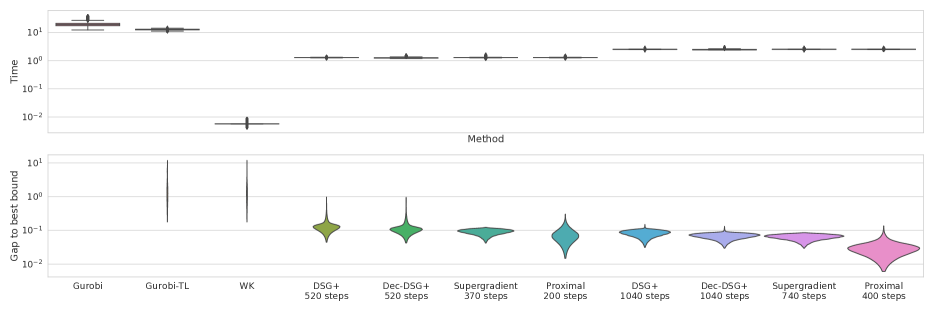
Figure 2: Distribution of runtime and gap to optimality on a network adversarially trained with the method by  Madry et al., (2018), on CIFAR-10 images. In both cases, lower is better. The width at a given value represents the proportion of problems for which this is the result. Gurobi always return the optimal solution so doesn’t appear on the optimality gap, but is always the highest runtime.

6.2 EXPERIMENTAL SETTING

In order to evaluate the performance of the proposed methods, we first perform a comparison in the quality and speed of bounds obtained by different methods in the context of incomplete verification ($\S$6.3). We then assess the effect of the various method-specific speed/accuracy trade-offs within a complete verification procedure ($\S$6.4).

For both sets of experiments, we report results using networks trained with different methodologies on the CIFAR-10 dataset. We compare the following algorithms:

• WK uses the method of Wong and Kolter, (2018). This is equivalent to a specific choice of $\bm{\rho}$.

• DSG+ corresponds to supergradient ascent on dual (2), the method by Dvijotham et al., (2018). We use the Adam (Kingma and Ba,, 2015) updates rules and decrease the step size linearly, similarly to the experiments of Dvijotham et al., (2018). We experimented with other step size schedules, like constant step size or $\frac{1}{t}$ schedules, which all performed worse.

• Dec-DSG+ is a direct application of Theorem 1: it obtains a dual solution for problem (2) via DSG+ and sets $\bm{\rho}=\bm{\mu}$ in problem (9) to obtain the final bounds.

• Supergradient is the first of the two solvers presented ($\S$5.1). It corresponds to supergradient ascent over problem (9). We use Adam updates as in DSG+.

• Proximal is the solver presented in $\S$5.2, performing proximal maximisation on problem (9). We limit the total number of inner iterations for each problem to $2$ (a single iteration is a full pass over the network layers).

• Gurobi is our gold standard method, employing the commercial black box solver Gurobi. All the problems are solved to optimality, providing us with the best result that our solver could achieve in terms of accuracy.

• Gurobi-TL is the time-limited version of the above, which stops at the first dual simplex iteration for which the total elapsed time exceeded that required by $400$ iterations of the proximal method.

We omit Interval Bound Propagation (Gowal et al.,, 2018, Mirman et al.,, 2018) from the comparisons as on average it performed significantly worse than WK on the networks we used: experimental results are provided in appendix G.1. For all of the methods above, as done in previous work for neural network verification (Lu and Kumar,, 2020, Bunel et al.,, 2020), we compute intermediate bounds (see appendix B) by taking the layer-wise best bounds output by Interval Propagation and WK. This holds true for both the incomplete and the complete verification experiments. Gurobi was run on $4$ CPUs for $\S$ 6.3 and on $1$ for $\S$ 6.4 in order to match the setting by Bunel et al., (2020), whereas all the other methods were run on a single GPU. While it may seem to lead to an unfair comparison, the flexibility and parallelism of the methods are a big part of their advantages over off-the-shelf solvers.

6.3 INCOMPLETE VERIFICATION

We investigate the effectiveness of the various methods for incomplete verification on images of the CIFAR-10 test set. For each image, we compute an upper bound on the robustness margin: the difference between the ground truth logit and all the other logits, under an allowed perturbation $\epsilon_{\text{verif}}$ in infinity norm of the inputs. If for any class the upper bound on the robustness margin is negative, then we are certain that the network is vulnerable against that adversarial perturbation. We measure the time to compute last layer bounds, and report the optimality gap compared to the best achieved solution.

As network architecture, we employ the small model used by Wong and Kolter, (2018) and whose structure is given in appendix G.1.1. We train the network against perturbations of a size up to $\epsilon_{\text{train}}=8/255$, and test for adversarial vulnerability on $\epsilon_{\text{verif}}=12/255$. This is done using adversarial training (Madry et al.,, 2018), based on an attacker using 50 steps of projected gradient descent to obtain the samples. Additional experiments for a network trained using standard stochastic gradient descent and cross entropy, with no robustness objective can be found in appendix G.1. For both supergradient methods (our Supergradient, and DSG+), we decrease the step size linearly from $\alpha=10^{-2}$ to $\alpha=10^{-4}$, while for Proximal, we employ momentum coefficient $\mu=0.3$ and, for all layers, linearly increase the weight of the proximal terms from $\eta=10^{1}$ to $\eta=5\times 10^{2}$ (see appendix C).

Figure 3: Pointwise comparison for a subset of the methods on the data presented in Figure 2. Each datapoint corresponds to a CIFAR image, darker colour shades mean higher point density. The dotted line corresponds to the equality and in both graphs, lower is better along both axes.

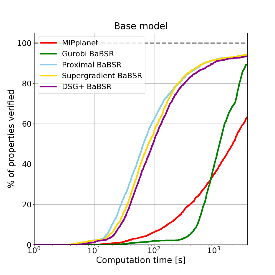
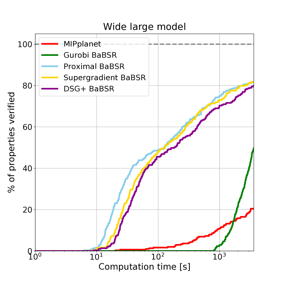
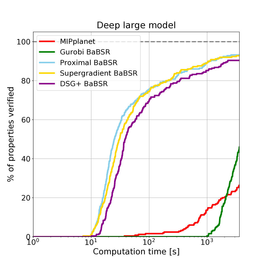
Figure 4: Cactus plots for the base, wide and deep models. For each, we compare the bounding methods and complete verification algorithms by plotting the percentage of solved properties as a function of runtime.

Figure 2 presents results as a distribution of runtime and optimality gap. WK by Wong and Kolter, (2018) performs a single pass over the network per optimization problem, which allows it to be extremely fast, but this comes at the cost of generating looser bounds. At the complete opposite end of the spectrum, Gurobi is extremely slow but provides the best achievable bounds. Dual iterative methods (DSG+, Supergradient, Proximal) allow the user to choose the trade-off between tightness and speed. In order to perform a fair comparison, we fixed the number of iterations for the various methods so that each of them would take the same average time (see Figure 3). This was done by tuning the iteration ratios on a subset of the images for the results in Figures 2, 3. Note that the Lagrangian Decomposition has a higher cost per iteration due to the more expensive computations related to the more complex primal feasible set. The cost of the proximal method is even larger due to the primal-dual updates and the optimal step size computation. For DSG+, Supergradient and Proximal, the improved quality of the bounds as compared to the non-iterative method WK shows that there are benefits in actually solving the best relaxation rather than simply evaluating looser bounds. Time-limiting Gurobi at the first iteration which exceeded the cost of $400$ Proximal iterations significantly worsens the produced bounds without a comparable cut in runtimes. This is due to the high cost per iteration of the dual simplex algorithm.

By looking at the distributions and at the point-wise comparisons in Figure 3, we can see that Supergradient yields consistently better bounds than DSG+. As both methods employ the Adam update rule (and the same hyper-parameters, which are optimal for both), we can conclude that operating on the Lagrangian Decomposition dual (1) produces better speed-accuracy trade-offs compared to the dual (2) by Dvijotham et al., (2018). This is in line with the expectations from Theorem 1. Furthermore, while a direct application of the Theorem (Dec-DSG+) does improve on the DSG+ bounds, operating on the Decomposition dual (1) is empirically more effective (see pointwise comparisons in appendix G.1). Finally, on average, the proximal algorithm yields better bounds than those returned by Supergradient, further improving on the DSG+ baseline. In particular, we stress that the support of optimality gap distribution is larger for Proximal, with a heavier tail towards better bounds.

6.4 COMPLETE VERIFICATION

Table 1: For base, wide and deep models, we compare average solving time, average number of solved sub-problems and the percentage of timed out properties. The best performing iterative method is highlighted in bold.

Base Wide Deep Method time(s) sub-problems $\%$Timeout time(s) sub-problems $\%$Timeout time(s) sub-problems $\%$Timeout Gurobi BaBSR $1588.651$ $1342.777$ $10.56$ $2912.246$ $630.864$ $50.66$ $3007.237$ $299.913$ $54.00$ MIPplanet $2035.565$ $36.37$ $3118.593$ $80.00$ $2997.115$ $73.60$ DSG+ BaBSR $426.554$ $5312.674$ $6.54$ $1048.594$ $4518.116$ $20.00$ $509.484$ $1992.345$ $9.60$ Supergradient BaBSR $377.104$ $5079.682$ $5.76$ $920.351$ $4069.894$ $18.00$ $390.367$ $1783.577$ $7.2$ Proximal BaBSR $368.876$ $4569.414$ $5.82$ $891.163$ $3343.601$ $18.00$ $384.984$ $1655.519$ $6.8$

We present results for complete verification. In this setting, our goal is to verify whether a network is robust to $\ell_{\infty}$ norm perturbations of radius $\epsilon_{\text{verif}}$. In order to do so, we search for a counter-example (an input point for which the output of the network is not the correct class) by minimizing the difference between the ground truth logit and a randomly chosen logit of images of the CIFAR-10 test set. If the minimum is positive, we have not succeeded in finding a counter-example, and the network is robust. In contrast to the previous section, we now seek to solve a nonconvex problem like (1) (where another layer representing the aforementioned difference has been added at the end) directly, rather than an approximation.

In order to perform the minimization exactly, we employ BaSBR, a Branch and Bound algorithm by Bunel et al., (2020). In short, Branch and Bound divides the verification domain into a number of smaller problems, for which it repeatedly computes upper and lower bounds. At every iteration, BaSBR picks the sub-problem with the lowest lower bound and creates two new sub-problems by fixing the most “impactful” ReLU to be passing or blocking. The impact of a ReLU is determined by estimating the change in the sub-problem’s output lower bound caused by making the ReLU non-ambiguous. Sub-problems which cannot contain the global lower bound are progressively discarded.

The computational bottleneck of Branch and Bound is the lower bounds computation, for which we will employ a subset of the methods in section 6.2. Specifically, we want to compare the performance of DSG+, Supergradient and Proximal with Gurobi (as employed in Bunel et al., (2020)). For this purpose, we run the various Branch and Bound implementations on the dataset employed by Lu and Kumar, (2020) to test their novel Branch and Bound splitting strategy. The dataset picks a non-correct class and a perturbation radius $\epsilon_{\text{verif}}$ for a subset of the CIFAR-10 test images, and runs Branch and Bound on three different convolutional network architectures of varying size: a “base” network, a “wide” network, and a “deep” network. Further details on the dataset and architectures are provided in appendix G.2.

We compare the Branch and Bound implementations with MIPplanet to provide an additional verification baseline. MIPplanet computes the global lower bound by using Gurobi to solve the Mixed-Integer Linear problem arising from the Planet relaxation (Bunel et al.,, 2020, Ehlers,, 2017). As explained in section 6.1, due to the highly parallelizable nature of the dual iterative algorithms, we are able to compute lower bounds for multiple sub-problems at once for DSG+, Supergradient and Proximal, whereas the domains are solved sequentially for Gurobi. The number of simultaneously solved sub-problems is $300$ for the base network, and $200$ for the wide and deep networks. Intermediate bound computations (see $\S$6.2) are performed in parallel as well, with smaller batch sizes to account for the larger width of intermediate layers (over which we batch as well). For both supergradient methods (our Supergradient, and DSG+), we decrease the step size linearly from $\alpha=10^{-3}$ to $\alpha=10^{-4}$, while for Proximal, we do not employ momentum and keep the weight of the proximal terms fixed to $\eta=10^{2}$ for all layers throughout the iterations. As in the previous section, the number of iterations for the bounding algorithms are tuned to employ roughly the same time: we use $100$ iterations for Proximal, $160$ for Supergradient, and $260$ for DSG+. For all three, the dual variables are initialized from the dual solution of the lower bound computation of the parent node in the Branch and Bound tree. We time-limit the experiments at one hour.

Consistently with the incomplete verification results in the last section, Figure 4 and Table 1 show that the Supergradient overperforms DSG+, confirming the benefits of our Lagrangian Decomposition approach. Better bounds decrease the number of sub-problems that Branch and Bound needs to solve, reducing the overall verification time. Furthermore, Proximal provides an additional increase in performance over DSG+, which is visible especially over the properties that are easier to verify. The gap between competing bounding methods increases with the size of the employed network, both in terms of layer width and network depth: at least an additional $2\%$ of the properties times out when using DSG+ on the larger networks. A more detailed experimental analysis of the base model data is presented in appendix G.2.

7 DISCUSSION

We have presented a novel dual approach to compute bounds over the activation of neural networks based on Lagrangian Decomposition. It provides significant benefits compared to off-the-shelf solvers and improves on both looser relaxations and on a previous method based on Lagrangian relaxation. As future work, it remains to investigate whether better complete verification results can be obtained by combining our supergradient and proximal methods. Furthermore, it would be interesting to see if similar derivations could be used to make tighter but more expensive relaxations computationally feasible. Improving the quality of bounds may allow the training of robust networks to avoid over-regularisation.

Acknowledgments

ADP was supported by the EPSRC Centre for Doctoral Training in Autonomous Intelligent Machines and Systems, grant EP/L015987/1. RB wishes to thank Leonard Berrada for helpful discussions on the convex hull of sigmoid activation functions.

Appendix A Sigmoid Activation function

This section describes the computation highlighted in the paper in the context where the activation function $\sigma\left(x\right)$ is the sigmoid function:

$$\sigma\left(x\right)=\frac{1}{1+e^{-x}}$$ (18)

A similar methodology to the ones described in this section could be used to adapt the method to work with other activation function such as hyperbolic tangent, but we won’t discuss it.

We will start with a reminders about some properties of the sigmoid activation function. It takes values between 0 and 1, with $\sigma\left(0\right)=0.5$. We can easily compute its derivatives:

$$\begin{split}\sigma^{\prime}\left(x\right)&=\sigma\left(x\right)\times(1-\sigma\left(x\right))\\ \sigma^{\prime\prime}\left(x\right)&=\sigma\left(x\right)\times(1-\sigma\left(x\right))\times\left(1-2\sigma\left(x\right)\right)\\ \end{split}$$ (19)

If we limit the domain of study to the negative inputs ($\left[-\infty,0\right]$), then the function $x\mapsto\sigma\left(x\right)$ is a convex function, as can be seen by looking at the sign of the second derivative over that domain. Similarly, if we limit the domain of study to the positive inputs ($\left[0,\infty\right]$), the function is concave.

(a) The upper bound is in Case 1, while the lower bound is in the special case of Case 2 with only one piece.

(b) The upper bound is in the special case of Case 2 with only one piece, while the lower bound is in Case 1.

(c) Both upper and lower bounds are in Case 2 with the two pieces visible.

Figure 5: Convex hull of the Sigmoid activation function for different input bound configurations.

A.1 Convex hull computation

In the context of ReLU, the convex hull of the activation function is given by equation(4c), as introduced by Ehlers, (2017). We will now derive it for sigmoid functions. Upper and lower bounds will be dealt in the same way, so our description will only focus on how to obtain the concave upper bound, limiting the activation function convex hull by above. The computation to derive the convex lower bound is equivalent.

Depending on the range of inputs over which the convex hull is taken, the form of the concave upper bound will change. We distinguish two cases.

Case 1: $\sigma^{\prime}\left(\mathbf{u}_{k}\right)\geq\frac{\sigma\left(\mathbf{u}_{k}\right)-\sigma\left(\mathbf{l}_{k}\right)}{\mathbf{u}_{k}-\mathbf{l}_{k}}$.

We will prove that in this case, the upper bound will be the line passing through the points $(\mathbf{l}_{k},\sigma\left(\mathbf{l}_{k}\right))$ and $(\mathbf{u}_{k},\sigma\left(\mathbf{l}_{k}\right))$. The equation of it is given by:

$$\phi_{\mathbf{u}_{k},\mathbf{l}_{k}}(\mathbf{x})=\frac{\sigma\left(\mathbf{u}_{k}\right)-\sigma\left(\mathbf{l}_{k}\right)}{\mathbf{u}_{k}-\mathbf{l}_{k}}\left(\mathbf{x}-\mathbf{l}_{k}\right)+\sigma\left(\mathbf{l}_{k}\right)$$ (20)

Consider the function $d(\mathbf{x})=\phi_{\mathbf{u}_{k},\mathbf{l}_{k}}(\mathbf{x})-\sigma\left(\mathbf{x}\right)$. To show that $\phi_{\mathbf{u}_{k},\mathbf{l}_{k}}$ is a valid upper bound, we need to prove that $\forall\mathbf{x}\in\left[\mathbf{l}_{k},\mathbf{u}_{k}\right],\ d(\mathbf{x})\geq 0$. We know that $d(\mathbf{l}_{k})=0$ and $d(\mathbf{u}_{k})=0$, and that $d$ is a continuous function. Its derivative is given by:

$$d^{\prime}(\mathbf{x})=\frac{\sigma\left(\mathbf{u}_{k}\right)-\sigma\left(\mathbf{l}_{k}\right)}{\mathbf{u}_{k}-\mathbf{l}_{k}}-\sigma\left(\mathbf{x}\right)(1-\sigma\left(\mathbf{x}\right)).$$ (21)

To find the roots of $d^{\prime}$, we can solve $d^{\prime}(\mathbf{x})=0$ for the value of $\sigma\left(\mathbf{x}\right)$ and then use the logit function to recover the value of $\mathbf{x}$. In that case, this is only a second order polynomial, so it can admit at most two roots.

We know that $\lim_{\mathbf{x}\to\infty}d^{\prime}(\mathbf{x})\geq 0$, and our hypothesis tells us that $d^{\prime}(\mathbf{u}_{k})\leq 0$. This means that at least one of the root lies necessarily beyond $\mathbf{u}_{k}$ and therefore, the derivative of $d$ change signs at most once on the $\left[\mathbf{l}_{k},\mathbf{u}_{k}\right]$ interval. If it never changes sign, it is monotonous. Given that the values taken at both extreme points are the same, $d$ being monotonous would imply that $d$ is constant, which is impossible. We therefore conclude that this means that the derivative change its sign exactly once on the interval, and is therefore unimodal. As we know that $d^{\prime}(\mathbf{u}_{k})\leq 0$, this indicates that $d$ is first increasing and then decreasing. As both extreme points have a value of zero, this means that $\forall\mathbf{x}\in\left[\mathbf{l}_{k},\mathbf{u}_{k}\right],\ d(x)\geq 0$.

From this result, we deduce that $\phi_{\mathbf{u}_{k},\mathbf{l}_{k}}$ is a valid upper bound of $\sigma$. As a linear function, it is concave by definition. Given that it constitutes the line between two points on the curve, all of its points necessarily belong to the convex hull. Therefore, it is not possible for a concave upper bound of the activation function to have lower values. This means that $\phi_{\mathbf{u}_{k},\mathbf{l}_{k}}$ defines the upper bounding part of the convex hull of the activation function.

Case 2: $\sigma^{\prime}\left(\mathbf{u}_{k}\right)\leq\frac{\sigma\left(\mathbf{u}_{k}\right)-\sigma\left(\mathbf{l}_{k}\right)}{\mathbf{u}_{k}-\mathbf{l}_{k}}$.

In this case, we will have to decompose the upper bound into two parts, defined as follows:

$$\phi_{\mathbf{u}_{k},\mathbf{l}_{k}}(\mathbf{x}) \frac{\sigma\left(\mathbf{t}_{k}\right)-\sigma\left(\mathbf{l}_{k}\right)}{\mathbf{t}_{k}-\mathbf{l}_{k}}\left(\mathbf{x}-\mathbf{l}_{k}\right)+\sigma\left(\mathbf{l}_{k}\right) \mathbf{x}\in\left[\mathbf{l}_{k},\mathbf{t}_{k}\right]$$ if (22a)

$$\phi_{\mathbf{u}_{k},\mathbf{l}_{k}}(\mathbf{x}) \sigma\left(\mathbf{x}\right) \mathbf{x}\in\left[\mathbf{t}_{k},\mathbf{u}_{k}\right]$$ if , (22b)

where $\mathbf{t}_{k}$ is defined as the point such that $\sigma^{\prime}\left(\mathbf{t}_{k}\right)=\frac{\sigma\left(\mathbf{t}_{k}\right)-\sigma\left(\mathbf{l}_{k}\right)}{\mathbf{t}_{k}-\mathbf{l}_{k}}$ and $\mathbf{t}_{k}>0$. The value of $\mathbf{t}_{k}$ can be computed by solving the equation $\sigma\left(\mathbf{t}_{k}\right)(1-\sigma\left(\mathbf{t}_{k}\right))=\frac{\sigma\left(\mathbf{t}_{k}\right)-\sigma\left(\mathbf{l}_{k}\right)}{\mathbf{t}_{k}-\mathbf{l}_{k}}$, which can be done using the Newton-Raphson method or a binary search. Note that this needs to be done only when defining the problem, and not at every iteration of the solver. In addition, the value of $\mathbf{t}_{k}$ is dependant only on $\mathbf{l}_{k}$ so it’s possible to start by building a table of the results at the desired accuracy and cache them.

Evaluating both pieces of the function of equation(22b) at $\mathbf{t}_{k}$ show that $\phi_{\mathbf{u}_{k},\mathbf{l}_{k}}$ is continuous. Both pieces are concave (for $\mathbf{x}\geq\mathbf{t}_{k}\geq 0$, $\sigma$ is concave) and they share a supergradient (the linear function of slope $\frac{\sigma\left(\mathbf{t}_{k}\right)-\sigma\left(\mathbf{l}_{k}\right)}{\mathbf{t}_{k}-\mathbf{l}_{k}}$) in $\mathbf{t}_{k}$, so $\phi_{\mathbf{u}_{k},\mathbf{l}_{k}}$ is a concave function. The proof we did for Case 1 can be duplicated to show that the linear component is the best concave upper bound that can be achieved over the interval $\left[\mathbf{l}_{k},\mathbf{t}_{k}\right]$. On the interval $\left[\mathbf{t}_{k},\mathbf{u}_{k}\right]$, $\phi_{\mathbf{u}_{k},\mathbf{l}_{k}}$ is equal to the activation function, so it is also an upper bound which can’t be improved upon. Therefore, $\phi_{\mathbf{u}_{k},\mathbf{l}_{k}}$ is the upper bounding part of the convex hull of the activation function.

Note that a special case of this happens when $\mathbf{l}_{k}\geq\mathbf{t}_{k}$. In which case, $\phi_{\mathbf{u}_{k},\mathbf{l}_{k}}$ consists of only equation (22b).

All cases are illustrated in Figure 5. Case 1 is shown in 5(a), where the upper bound contains only the linear upper bound. Case 2 with both segments is visible in Figure5(c), with the cutoff points $tb_{k}$ highlighted by a green dot, and the special case with $\mathbf{l}_{k}\geq\mathbf{t}_{k}$ is demonstrated in Figure 5(b).

A.2 Solving the $\mathcal{P}_{k}$ subproblems over sigmoid activation

As a reminder, the problem that needs to be solved is the following (where $\mathbf{c}_{k+1}=-\bm{\rho}_{k+1}$, $\mathbf{c}_{k}=\bm{\rho}_{k}$):

$$\begin{split}[\mathbf{\hat{x}}_{B,k},\mathbf{\hat{x}}_{A,k+1}]=\operatorname*{\arg\!\min}_{\mathbf{\hat{z}}_{B,k},\mathbf{\hat{z}}_{A,k+1}}&\quad\mathbf{c}_{k}^{T}\mathbf{\hat{z}}_{B,k}+\mathbf{c}_{k+1}^{T}\mathbf{\hat{z}}_{A,k+1}\\ \text{s.t }&\quad\mathbf{l}_{k}\leq\mathbf{\hat{z}}_{B,k}\leq\mathbf{u}_{k}\\ &\quad\texttt{cvx\_hull}_{\sigma}\left(\mathbf{\hat{z}}_{B,k},\mathbf{z}_{k},\mathbf{l}_{k},\mathbf{u}_{k}\right)\\ &\quad\mathbf{\hat{z}}_{A,k+1}=W_{k+1}\mathbf{z}_{k}+\mathbf{b}_{k+1},\end{split}$$ (23)

where cvx_hull is defined either by equations (20) or (22b). In this case, we will still be able to compute a closed form solution.

We will denote $\phi_{\mathbf{u}_{k},\mathbf{l}_{k}}$ and $\psi_{\mathbf{u}_{k},\mathbf{l}_{k}}$ the upper and lower bound functions defining the convex hull of the sigmoid function, which can be obtained as described in the previous subsection. If we use the last equality constraint of Problem (23) to replace the $\mathbf{\hat{z}}_{A,k+1}$ term in the objective function, we obtain $\mathbf{c}_{k}^{T}\mathbf{\hat{z}}_{B,k}+\mathbf{c}_{k+1}^{T}W_{k+1}\mathbf{z}_{k}$. Depending on the sign of $\mathbf{c}_{k+1}^{T}W_{k+1}$, $\mathbf{z}_{k}$ will either take the value $\phi_{\mathbf{u}_{k},\mathbf{l}_{k}}$ or $\psi_{\mathbf{u}_{k},\mathbf{l}_{k}}$, resulting in the following problem:

$$\begin{split}\min_{\mathbf{\hat{z}}_{B,k}}\quad&\mathbf{c}^{T}_{k}\mathbf{\hat{z}}_{B,k}+\left[\mathbf{c}^{T}_{k+1}W_{k+1}\right]_{-}\phi_{\mathbf{u}_{k},\mathbf{l}_{k}}\left(\mathbf{\hat{z}}_{B,k}\right)+\left[\mathbf{c}^{T}_{k+1}W_{k+1}\right]_{+}\psi_{\mathbf{u}_{k},\mathbf{l}_{k}}\left(\mathbf{\hat{z}}_{B,k}\right)\\ \text{s.t }&\quad\mathbf{l}_{k}\leq\mathbf{\hat{z}}_{B,k}\leq\mathbf{u}_{k}.\end{split}$$ (24)

To solve this problem, several observations can be made: First of all, at that point, the optimisation decomposes completely over the components of $\mathbf{\hat{z}}_{B,k}$ so all problems can be solved independently from each other. The second observation is that to solve this problem, we can decompose the minimisation over the whole range $\left[\mathbf{l}_{k},\mathbf{u}_{k}\right]$ into a set of minimisation over the separate pieces, and then returning the minimum corresponding to the piece producing the lowest value.

The minimisation over the pieces can be of two forms. Both bounds can be linear (such as between the green dotted lines in Figure 5(c)), in which case the problem is easy to solve by looking at the signs of the coefficient of the objective function. The other option is that one of the bound will be equal to the activation function (such as in Figures 5(a) or 5(b), or in the outer sections of Figure 5(c)), leaving us with a problem of the form:

$$\begin{split}\min_{\mathbf{\hat{z}}_{B,k}}\quad&\mathbf{c}_{\text{lin}}^{T}\mathbf{\hat{z}}_{B,k}+\mathbf{c}_{\sigma}^{T}\sigma\left(\mathbf{\hat{z}}_{B,k}\right)\\ &\mathbf{l}\leq\mathbf{\hat{z}}_{B,k}\leq\mathbf{u},\end{split}$$ (25)

where $\mathbf{l}$, $\mathbf{u}$, $\mathbf{c}_{\text{lin}}$ and $\mathbf{c}_{\sigma}$ will depend on what part of the problem we are trying to solve.

This is a convex problem so the value will be reached either at the extremum of the considered domain ($\mathbf{l}$ or $\mathbf{u}$), or it will be reached at the points where the derivative of the objective functions cancels. This corresponds to the roots of $\mathbf{c}_{\text{lin}}+\mathbf{c}_{\sigma}^{T}\sigma\left(\mathbf{\hat{z}}_{B,k}\right)(1-\sigma\left(\mathbf{\hat{z}}_{B,k}\right))$. Provided that $1+\frac{4\mathbf{c}_{\text{lin}}}{\mathbf{c}_{\sigma}}\geq 0$, the possible roots will be given by $\sigma^{-1}\left(\frac{1\pm\sqrt{1+\frac{4\mathbf{c}_{\text{lin}}}{\mathbf{c}_{\sigma}}}}{2}\right)$, with $\sigma^{-1}$ being the logit function, the inverse of the sigmoid function $\left(\sigma^{-1}(\mathbf{x})=\log\left(\frac{\mathbf{x}}{1-\mathbf{x}}\right)\right)$. To solve problem (25), we evaluate its objective function at the extreme points ($\mathbf{l}$ and $\mathbf{u}$) and at those roots if they are in the feasible domain, and return the point corresponding to the minimum score achieved. With this method, we can solve the $\mathcal{P}_{k}$ subproblems even when the activation function is a sigmoid.

Appendix B Intermediate bounds

Intermediate bounds are obtained by solving a relaxation of (1) over subsets of the network. Instead of defining the objective function on the activation of layer $n$, we define it over $\mathbf{\hat{z}}_{k}$, iteratively for $k\in[1..n-1]$. Computing intermediate bounds with the same relaxation would be the computational cost of this approach: we need to solve two LPs for each of the neurons in the network, and even if (differently from off-the-shelf LP solvers) our method allows for easy parallelization within each layer, the layers need to be tackled sequentially. Therefore, depending on the computational budget, the employed relaxation for intermediate bounds might be looser than (3) or (2): for instance, the one by Wong and Kolter, (2018).

Appendix C Implementation details for Proximal method

We provide additional details for the implementation of the proximal method. We start with the optimal step size computation, define our block-coordinate updates for the primal variables, and finally provide some insight on acceleration.

C.1 Optimal Step Size Computation

Having obtained the conditional gradients $\mathbf{\hat{x}}_{k}\ \forall k\in[0..n-1]$ for our problem, we need to decide a step size. Computing the optimal step size amounts to solving a one dimensional quadratic problem:

$$\gamma^{*}=\operatorname*{\arg\!\min}_{\gamma\in\left[0,1\right]}\mathcal{L}(\gamma\mathbf{\hat{x}}+(1-\gamma)\mathbf{\hat{z}},\bm{\rho}).$$ (26)

Computing the gradient with regards to $\gamma$ and setting it to 0 will return the optimal step size. Denoting the gradient of the Augmented Lagrangian (17) with respect to $(\mathbf{\hat{z}}_{B,k}-\mathbf{\hat{z}}_{A,k})$ as $\nabla_{(\mathbf{\hat{z}}_{B,k}-\mathbf{\hat{z}}_{A,k})}\mathcal{L}\left(\mathbf{\hat{z}},\bm{\rho}\right)=\bm{\rho}_{k}+\frac{\mathbf{\hat{z}}_{B,k}-\mathbf{\hat{z}}_{A,k}}{\eta_{k}}=\mathbf{g}_{k}$, this gives us the following formula:

$$\gamma^{*}=\texttt{clamp}_{[0,1]}\left(-\frac{\left(\mathbf{\hat{x}}_{A,n}-\mathbf{\hat{z}}_{A,n}\right)+\sum_{k}\mathbf{g}_{k}^{T}\left(\mathbf{\hat{x}}_{B,k}-\mathbf{\hat{z}}_{B,k}-\mathbf{\hat{x}}_{A,k}+\mathbf{\hat{z}}_{A,k}\right)}{\sum_{k}\frac{1}{\eta_{k}}\|\mathbf{\hat{x}}_{B,k}-\mathbf{\hat{z}}_{B,k}-\mathbf{\hat{x}}_{A,k}+\mathbf{\hat{z}}_{A,k}\|^{2}}\right)$$ (27)

C.2 Gauss-Seidel style updates

At iteration $t$, the Frank-Wolfe step takes the following form:

$$\mathbf{\hat{z}}^{t+1}=\gamma^{*}\mathbf{x}+(1-\gamma^{*})\mathbf{\hat{z}}^{t}$$ (28)

where the update is performed on the variables associated to all the network neurons at once.

As the Augmented Lagrangian (17) is smooth in the primal variables, we can take a conditional gradient step after each $\mathbf{\hat{x}}_{k}$ computation, resulting in Gauss-Seidel style updates (as opposed to Jacobi style updates 28) (Bertsekas and Tsitsiklis,, 1989). As the values of the primals at following layers are inter-dependent through the gradient of the Augmented Lagrangian, these block-coordinate updates will result in faster convergence. The updates become:

$$\mathbf{\hat{z}}_{k}^{t+1}=\gamma_{k}^{*}\mathbf{\hat{x}}_{k}+(1-\gamma_{k}^{*})\mathbf{\hat{z}}_{k}^{t}$$ (29)

where the optimal step size is given by:

$$\gamma_{k}^{*}=\texttt{clamp}_{[0,1]}\left(-\frac{\mathbf{g}_{k}^{T}\left(\mathbf{\hat{x}}_{B,k}-\mathbf{\hat{z}}_{B,k})+\mathbf{g}_{k+1}^{T}(\mathbf{\hat{z}}_{A,k+1}-\mathbf{\hat{x}}_{A,k+1})\right)}{\frac{1}{\eta_{k}}\|\mathbf{\hat{x}}_{B,k}-\mathbf{\hat{z}}_{B,k}\|^{2}+\frac{1}{\eta_{k+1}}\|\mathbf{\hat{z}}_{A,k+1}-\mathbf{\hat{x}}_{A,k+1}\|^{2}}\right)$$ (30)

with the special cases $\mathbf{\hat{x}}_{B,0}=\mathbf{\hat{z}}_{B,0}=0$ and:

$$\gamma_{n-1}^{*}=\texttt{clamp}_{[0,1]}\left(-\frac{\mathbf{g}_{n-1}^{T}\left(\mathbf{\hat{x}}_{B,n-1}-\mathbf{\hat{z}}_{B,n-1})+(\mathbf{\hat{x}}_{A,n}-\mathbf{\hat{z}}_{A,n})\right)}{\frac{1}{\eta_{n-1}}\|\mathbf{\hat{x}}_{B,n-1}-\mathbf{\hat{z}}_{B,n-1}\|^{2}}\right)$$ (31)

C.3 Momentum

The supergradient methods that we implemented both for our dual (9) and for (2) by Dvijotham et al., (2018) rely on Adam (Kingma and Ba,, 2015) to speed-up convergence. Inspired by its presence in Adam, and by the work on accelerating proximal methods Lin et al., (2017), Salzo and Villa, (2012), we apply momentum on the proximal updates.

By closely looking at equation (16), we can draw a similarity between the dual update in the proximal algorithm and supergradient descent. The difference is that the former operation takes place after a closed-form minimization of the linear inner problem in $\mathbf{\hat{z}}_{A},\mathbf{\hat{z}}_{B}$, whereas the latter after some steps of an optimization algorithm that solves the quadratic form of the Augmented Lagrangian (17). We denote the (approximate) argmin of the Lagrangian at the $t$-th iteration of the proximal method (method of multipliers) by $\mathbf{\hat{z}}^{t,\dagger}$.

Thanks to the aforementioned similarity, we can keep an exponential average of the gradient-like terms with parameter $\mu\in[0,1]$ and adopt momentum for the dual update, yielding:

$$\begin{split}\bm{\pi}_{k}^{t+1}&=\mu\bm{\pi}_{k}^{t}+\frac{\mathbf{\hat{z}}^{t,\dagger}_{B,k}-\mathbf{\hat{z}}^{t,\dagger}_{A,k}}{\eta_{k}}\\ \bm{\rho}_{k}^{t+1}&=\bm{\rho}_{k}^{t}+\bm{\pi}_{k}^{t+1}\end{split}$$ (32)

As, empirically, a decaying step size has a positive effect on Adam, we adopt the same strategy for the proximal algorithm as well, resulting in an increasing $\eta_{k}$. The augmented Lagrangian then becomes:

$$\begin{split}\left[\mathbf{z}^{t},\mathbf{\hat{z}}^{t}\right]\ =\smash{\operatorname*{\arg\!\min}_{\mathbf{z},\mathbf{\hat{z}}}}\,\mathcal{L}\left(\mathbf{\hat{z}},\bm{\rho}^{t}\right)&\quad\text{s.t. }\mathcal{P}_{0}(\mathbf{z}_{0},\mathbf{\hat{z}}_{A,1});\quad\mathcal{P}_{k}(\mathbf{\hat{z}}_{B,k},\mathbf{\hat{z}}_{A,k+1})\ \quad k\in\left[1..n-1\right]\\ \text{where }\mathcal{L}\left(\mathbf{\hat{z}},\bm{\rho}\right)=\ &\Bigg{[}\mathbf{\hat{z}}_{A,n}+\sum_{k=1..n-1}\bm{\rho}_{k}^{T}\left(\mathbf{\hat{z}}_{B,k}-\mathbf{\hat{z}}_{A,k}\right)+\sum_{k=1..n-1}\frac{1}{2\eta_{k}}\|\mathbf{\hat{z}}_{B,k}-\mathbf{\hat{z}}_{A,k}\|^{2}\\ &\ \ -\sum_{k=1..n-1}\quad\frac{\eta_{k}}{2}\|\mu\bm{\pi}_{k}\|^{2}\Bigg{]}.\end{split}$$ (33)

We point out that the Augmented Lagrangian’s gradient $\nabla_{(\mathbf{\hat{z}}_{B,k}-\mathbf{\hat{z}}_{A,k})}\mathcal{L}\left(\mathbf{\hat{z}},\bm{\rho}\right)$ remains unvaried with respect to the momentum-less solver hence, in practice, the main change is the dual update formula (32).

Appendix D Algorithm summary

We provide high level summaries of our solvers: supergradient (Algorithm 1) and proximal (Algorithm 2).

For both methods, we decompose problem (3) into several subset of constraints, duplicate the variables to make the subproblems independent, and enforce their consistency by introducing dual variables $\bm{\rho}$, which we are going to optimize. This results in problem (9), which we solve using one of the two algorithms. Our initial dual solution is given by the algorithm of Wong and Kolter, (2018). The details can be found in Appendix F.

Algorithm 1 Supergradient method

1:function subg_compute_bounds($\{W_{k},\mathbf{b}_{k},\mathbf{l}_{k},\mathbf{u}_{k}\}_{k=1..n}$)

2:   Initialise dual variables $\bm{\rho}$ using the algo of Wong and Kolter, (2018)

3:   for $\mathtt{nb\_iterations}$ do

4:      $\mathbf{\hat{z}}^{*}\leftarrow$ inner minimization using $\S$5.1.1 and $\S$5.1.2

5:      Compute supergradient using $\nabla_{\bm{\rho}}q(\bm{\rho}^{t})=\mathbf{\hat{z}}_{B}^{*}-\mathbf{\hat{z}}_{A}^{*}$

6:      $\bm{\rho}^{t+1}\leftarrow$ Adam’s update rule Kingma and Ba, (2015)

7:   end for

8:   return $q(\bm{\rho})$

9:end function

The structure of our employed supergradient method is relatively simple. We iteratively minimize over the primal variables (line 4) in order to compute the supergradient, which is then used to update the dual variables through the Adam update (line 6).

Algorithm 2 Proximal method

1:function prox_compute_bounds($\{W_{k},b_{k},l_{k},u_{k}\}_{k=1..n}$)

2:   Initialise dual variables $\bm{\rho}$ using the algo of Wong and Kolter, (2018)

3:   Initialise primal variables $\mathbf{\hat{z}}$ at the conditional gradient of $\bm{\rho}$

4:   for $\mathtt{nb\_outer\_iterations}$ do

5:      Update dual variables using equation (16) or (32)

6:      for $\mathtt{nb\_inner\_iterations}$ do

7:         for $k\in[0..n-1]$ do

8:            Compute layer conditional gradient $[\mathbf{\hat{x}}_{k}]$ using using $\S$5.1.1 and $\S$5.1.2

9:            Compute layer optimal step size $\gamma_{k}^{*}$ using (27)

10:            $\begin{array}[]{l}\text{Update layer primal variables:}\\ \qquad\mathbf{\hat{z}}_{k}=\gamma_{k}^{*}\mathbf{\hat{x}}_{k}+(1-\gamma_{k}^{*})\mathbf{\hat{z}}_{k}\\ \end{array}$

11:         end for

12:      end for

13:   end for

14:   return $q(\bm{\rho})$

15:end function

The proximal method, instead alternates updates to the dual variables (applying the updates from (16); line 5) and to the primal variables (update of (17); lines 6 to 12). The inner minimization problem is solved only approximately, using the Frank-Wolfe algorithm (line 10), applied in a block-coordinate fashion over the network layers (line 7). We have closed form solution for both the conditional gradient (line 8) and the optimal step-size (line 9).

Appendix E Comparison between the duals

We will show the relation between the decomposition done by Dvijotham et al., (2018) and the one proposed in this paper. We will show that, in the context of ReLU activation functions, from any dual solution of their dual providing a bound, our dual provides a better bound.

Theorem.

Let us assume $\sigma(\mathbf{\hat{z}}_{k})=\max(\mathbf{0},\mathbf{\hat{z}}_{k})$. For any solution $\bm{\mu},\bm{\lambda}$ of dual (2) by Dvijotham et al., (2018) yielding bound $d(\bm{\mu},\bm{\lambda})$, it holds that $q(\bm{\mu})\geq d(\bm{\mu},\bm{\lambda})$.

Proof.

We start by reproducing the formulation that Dvijotham et al., (2018) uses, which we slightly modify in order to have a notation more comparable to ours. With our convention, doing the decomposition to obtain Problem (6) in (Dvijotham et al.,, 2018) would give:

$$\begin{split}\min_{\mathbf{z},\mathbf{\hat{z}}}&\quad W_{n}\mathbf{z}_{n-1}+\mathbf{b}_{n}+\sum_{k=1}^{n-1}\bm{\mu}_{k}^{T}\left(\mathbf{\hat{z}}_{k}-W_{k}\mathbf{z}_{k-1}-\mathbf{b}_{k}\right)+\sum_{k=1}^{n-1}\bm{\lambda}_{k}^{T}\left(\mathbf{z}_{k}-\sigma(\mathbf{\hat{z}}_{k})\right)\\ \text{such that }\quad&\mathbf{l}_{k}\leq\mathbf{\hat{z}}_{k}\leq\mathbf{u}_{k}\qquad\qquad\text{for }k\in\left[1,n-1\right]\\ &\sigma(\mathbf{l}_{k})\leq\mathbf{z}_{k}\leq\sigma(\mathbf{u}_{k})\qquad\text{for }k\in\left[1,n-1\right]\\ &\mathbf{z}_{0}\in\mathcal{C}\end{split}$$ (34)

Decomposing it, in the same way that Dvijotham et al., (2018) do it in order to obtain their equation (7), we obtain

$$\begin{split}&\mathbf{b}_{n}-\sum_{k=1}^{n-1}\bm{\mu}_{k}^{T}\mathbf{b}_{k}+\sum_{k=1}^{n-1}\min_{\mathbf{\hat{z}}_{k}\in[\mathbf{l}_{k},\mathbf{u}_{k}]}\left(\bm{\mu}_{k}^{T}\mathbf{\hat{z}}_{k}-\bm{\lambda}_{k}^{T}\sigma(\mathbf{\hat{z}}_{k})\right)\\ &\qquad+\sum_{k=1}^{n-1}\min_{\mathbf{z}_{k}\in[\sigma\left(\mathbf{l}_{k}\right),\sigma\left(\mathbf{u}_{k}\right)]}\left(-\bm{\mu}_{k+1}^{T}W_{k+1}\mathbf{z}_{k}+\bm{\lambda}_{k}^{T}\mathbf{z}_{k}\right)+\min_{\mathbf{z}_{0}\in\mathcal{C}}-\bm{\mu}_{1}^{T}W_{1}\mathbf{z}_{0}.\end{split}$$ (35)

(with the convention that $\bm{\mu}_{n}=-I$)

As a reminder, the formulation of our dual (9) is:

$$\begin{split}q\left(\bm{\rho}\right)=\text{min }_{\mathbf{z},\mathbf{\hat{z}}}\ &\mathbf{\hat{z}}_{A,n}+\Sigma_{k=1..n-1}\bm{\rho}_{k}^{T}\left(\mathbf{\hat{z}}_{B,k}-\mathbf{\hat{z}}_{A,k}\right)\\ \text{s.t. }\quad&\mathcal{P}_{0}(\mathbf{z}_{0},\mathbf{\hat{z}}_{A,1});\quad\mathcal{P}_{k}(\mathbf{\hat{z}}_{B,k},\mathbf{\hat{z}}_{A,k+1})\qquad\text{for }k\in\left[1..n-1\right]\\ \end{split}$$ (36)

which can be decomposed as:

$$\begin{split}q\left(\bm{\rho}\right)=\sum_{k=1}^{n-1}&\left(\min_{\begin{array}[]{c}\mathbf{\hat{z}}_{B,k},\mathbf{\hat{z}}_{A,k+1}\\ \in\mathcal{P}_{k}\left(\cdot,\cdot\right)\end{array}}\bm{\rho}_{k}^{T}\mathbf{\hat{z}}_{B,k}\ -\ \bm{\rho}_{k+1}^{T}\mathbf{\hat{z}}_{A,k+1}\right)+\min_{\begin{array}[]{c}\mathbf{z}_{0},\mathbf{\hat{z}}_{A,1}\\ \in\mathcal{P}_{0}\left(\cdot,\cdot\right)\end{array}}-\bm{\rho}_{1}^{T}\mathbf{\hat{z}}_{A,1},\end{split}$$ (37)

with the convention that $\bm{\rho}_{n}=-I$. We will show that when we chose the dual variables such that

$$\bm{\rho}_{k}=\bm{\mu}_{k},$$ (38)

we obtain a tighter bound than the ones given by (35).

We will start by showing that the term being optimised over $\mathcal{P_{0}}$ is equivalent to some of the terms in (35):

$$\min_{\mathchoice{\hbox to0.0pt{\hss$\displaystyle{\begin{array}[]{c}\mathbf{z}_{0},\mathbf{\hat{z}}_{A,1}\\ \in\mathcal{P}_{0}\left(\cdot,\cdot\right)\end{array}}$\hss}}{\hbox to0.0pt{\hss$\textstyle{\begin{array}[]{c}\mathbf{z}_{0},\mathbf{\hat{z}}_{A,1}\\ \in\mathcal{P}_{0}\left(\cdot,\cdot\right)\end{array}}$\hss}}{\hbox to0.0pt{\hss$\scriptstyle{\begin{array}[]{c}\mathbf{z}_{0},\mathbf{\hat{z}}_{A,1}\\ \in\mathcal{P}_{0}\left(\cdot,\cdot\right)\end{array}}$\hss}}{\hbox to0.0pt{\hss$\scriptscriptstyle{\begin{array}[]{c}\mathbf{z}_{0},\mathbf{\hat{z}}_{A,1}\\ \in\mathcal{P}_{0}\left(\cdot,\cdot\right)\end{array}}$\hss}}}-\bm{\rho}_{1}^{T}\mathbf{\hat{z}}_{A,1}=\min_{\mathchoice{\hbox to0.0pt{\hss$\displaystyle{\begin{array}[]{c}\mathbf{z}_{0},\mathbf{\hat{z}}_{A,1}\\ \in\mathcal{P}_{0}\left(\cdot,\cdot\right)\end{array}}$\hss}}{\hbox to0.0pt{\hss$\textstyle{\begin{array}[]{c}\mathbf{z}_{0},\mathbf{\hat{z}}_{A,1}\\ \in\mathcal{P}_{0}\left(\cdot,\cdot\right)\end{array}}$\hss}}{\hbox to0.0pt{\hss$\scriptstyle{\begin{array}[]{c}\mathbf{z}_{0},\mathbf{\hat{z}}_{A,1}\\ \in\mathcal{P}_{0}\left(\cdot,\cdot\right)\end{array}}$\hss}}{\hbox to0.0pt{\hss$\scriptscriptstyle{\begin{array}[]{c}\mathbf{z}_{0},\mathbf{\hat{z}}_{A,1}\\ \in\mathcal{P}_{0}\left(\cdot,\cdot\right)\end{array}}$\hss}}}-\bm{\mu}_{1}^{T}\mathbf{\hat{z}}_{A,1}=-\bm{\mu}_{1}^{T}\mathbf{b}_{1}+\min_{\mathbf{z}_{0}\in\mathcal{C}}-\bm{\mu}_{1}^{T}W_{1}\mathbf{z}_{0}$$ (39)

The first equality is given by the replacement formula (38), while the second one is given by performing the replacement of $\mathbf{\hat{z}}_{A,1}$ with his expression in $\mathcal{P}_{0}$

We will now obtain a lower bound of the term being optimised over $\mathcal{P}_{k}$. Let’s start by plugging in the values using the formula (38) and replace the value of $\mathbf{\hat{z}}_{A,k+1}$ using the constraint.

$$\min_{\mathchoice{\hbox to0.0pt{\hss$\displaystyle{\begin{array}[]{c}\mathbf{\hat{z}}_{B,k},\mathbf{\hat{z}}_{A,k+1}\\ \in\mathcal{P}_{k}\left(\cdot,\cdot\right)\end{array}}$\hss}}{\hbox to0.0pt{\hss$\textstyle{\begin{array}[]{c}\mathbf{\hat{z}}_{B,k},\mathbf{\hat{z}}_{A,k+1}\\ \in\mathcal{P}_{k}\left(\cdot,\cdot\right)\end{array}}$\hss}}{\hbox to0.0pt{\hss$\scriptstyle{\begin{array}[]{c}\mathbf{\hat{z}}_{B,k},\mathbf{\hat{z}}_{A,k+1}\\ \in\mathcal{P}_{k}\left(\cdot,\cdot\right)\end{array}}$\hss}}{\hbox to0.0pt{\hss$\scriptscriptstyle{\begin{array}[]{c}\mathbf{\hat{z}}_{B,k},\mathbf{\hat{z}}_{A,k+1}\\ \in\mathcal{P}_{k}\left(\cdot,\cdot\right)\end{array}}$\hss}}}\left(\bm{\rho}_{k}^{T}\mathbf{\hat{z}}_{B,k}\ -\ \bm{\rho}_{k+1}^{T}\mathbf{\hat{z}}_{A,k+1}\right)=-\bm{\mu}_{k+1}^{T}\mathbf{b}_{k+1}+\qquad\min_{\mathchoice{\hbox to0.0pt{\hss$\displaystyle{\begin{array}[]{l}\qquad\mathbf{\hat{z}}_{B,k}\in[\mathbf{l}_{k},\mathbf{u}_{k}]\\ \qquad\texttt{cvx\_hull}(\mathbf{\hat{z}}_{B,k},\mathbf{z}_{k})\end{array}}$\hss}}{\hbox to0.0pt{\hss$\textstyle{\begin{array}[]{l}\qquad\mathbf{\hat{z}}_{B,k}\in[\mathbf{l}_{k},\mathbf{u}_{k}]\\ \qquad\texttt{cvx\_hull}(\mathbf{\hat{z}}_{B,k},\mathbf{z}_{k})\end{array}}$\hss}}{\hbox to0.0pt{\hss$\scriptstyle{\begin{array}[]{l}\qquad\mathbf{\hat{z}}_{B,k}\in[\mathbf{l}_{k},\mathbf{u}_{k}]\\ \qquad\texttt{cvx\_hull}(\mathbf{\hat{z}}_{B,k},\mathbf{z}_{k})\end{array}}$\hss}}{\hbox to0.0pt{\hss$\scriptscriptstyle{\begin{array}[]{l}\qquad\mathbf{\hat{z}}_{B,k}\in[\mathbf{l}_{k},\mathbf{u}_{k}]\\ \qquad\texttt{cvx\_hull}(\mathbf{\hat{z}}_{B,k},\mathbf{z}_{k})\end{array}}$\hss}}}\quad\left(\bm{\mu}_{k}^{T}\mathbf{\hat{z}}_{B,k}\ -\ \bm{\mu}_{k+1}^{T}W_{k+1}\mathbf{z}_{k}\right)\\$$ (40)

Focusing on the second term that contains the minimization over the convex hull, we will obtain a lower bound. It is important, at this stage, to recall that, as seen in section 5.1.2, the minimum of the second term can either be one of the three vertices of the triangle in Figure 1 (ambiguous ReLU), the $\mathbf{\hat{z}}_{B,k}=\mathbf{z}_{k}$ line (passing ReLU), or the $(\mathbf{\hat{z}}_{B,k}=\mathbf{0},\mathbf{z}_{k}=\mathbf{0})$ triangle vertex (blocking ReLU). We will write $(\mathbf{\hat{z}}_{B,k},\mathbf{z}_{k})\in\texttt{ReLU\_sol}(\mathbf{\hat{z}}_{B,k},\mathbf{z}_{k},\mathbf{l}_{k},\mathbf{u}_{k})$.

We can add a term $\bm{\lambda}_{k}^{T}(\sigma\left(\mathbf{\hat{z}}_{k}\right)-\sigma\left(\mathbf{\hat{z}}_{k}\right))=0$ and obtain:

$$\begin{split}&\min_{\begin{array}[]{c}\mathbf{\hat{z}}_{B,k}\in[\mathbf{l}_{k},\mathbf{u}_{k}]\\ \mathchoice{\hbox to0.0pt{\hss$\displaystyle{\texttt{cvx\_hull}(\mathbf{\hat{z}}_{B,k},\mathbf{z}_{k})}$\hss}}{\hbox to0.0pt{\hss$\textstyle{\texttt{cvx\_hull}(\mathbf{\hat{z}}_{B,k},\mathbf{z}_{k})}$\hss}}{\hbox to0.0pt{\hss$\scriptstyle{\texttt{cvx\_hull}(\mathbf{\hat{z}}_{B,k},\mathbf{z}_{k})}$\hss}}{\hbox to0.0pt{\hss$\scriptscriptstyle{\texttt{cvx\_hull}(\mathbf{\hat{z}}_{B,k},\mathbf{z}_{k})}$\hss}}\end{array}}\left(\bm{\mu}_{k}^{T}\mathbf{\hat{z}}_{B,k}\ -\ \bm{\mu}_{k+1}^{T}W_{k+1}\mathbf{z}_{k}\right)\\ =&\min_{\begin{array}[]{c}\mathbf{\hat{z}}_{B,k}\in[\mathbf{l}_{k},\mathbf{u}_{k}]\\ \mathchoice{\hbox to0.0pt{\hss$\displaystyle{\texttt{ReLU\_sol}(\mathbf{\hat{z}}_{B,k},\mathbf{z}_{k},\mathbf{l}_{k},\mathbf{u}_{k})}$\hss}}{\hbox to0.0pt{\hss$\textstyle{\texttt{ReLU\_sol}(\mathbf{\hat{z}}_{B,k},\mathbf{z}_{k},\mathbf{l}_{k},\mathbf{u}_{k})}$\hss}}{\hbox to0.0pt{\hss$\scriptstyle{\texttt{ReLU\_sol}(\mathbf{\hat{z}}_{B,k},\mathbf{z}_{k},\mathbf{l}_{k},\mathbf{u}_{k})}$\hss}}{\hbox to0.0pt{\hss$\scriptscriptstyle{\texttt{ReLU\_sol}(\mathbf{\hat{z}}_{B,k},\mathbf{z}_{k},\mathbf{l}_{k},\mathbf{u}_{k})}$\hss}}\end{array}}\left(\bm{\mu}_{k}^{T}\mathbf{\hat{z}}_{B,k}\ -\ \bm{\mu}_{k+1}^{T}W_{k+1}\mathbf{z}_{k}\right)\\ =&\min_{\begin{array}[]{c}\mathbf{\hat{z}}_{B,k}\in[\mathbf{l}_{k},\mathbf{u}_{k}]\\ \mathchoice{\hbox to0.0pt{\hss$\displaystyle{\texttt{ReLU\_sol}(\mathbf{\hat{z}}_{B,k},\mathbf{z}_{k},\mathbf{l}_{k},\mathbf{u}_{k})}$\hss}}{\hbox to0.0pt{\hss$\textstyle{\texttt{ReLU\_sol}(\mathbf{\hat{z}}_{B,k},\mathbf{z}_{k},\mathbf{l}_{k},\mathbf{u}_{k})}$\hss}}{\hbox to0.0pt{\hss$\scriptstyle{\texttt{ReLU\_sol}(\mathbf{\hat{z}}_{B,k},\mathbf{z}_{k},\mathbf{l}_{k},\mathbf{u}_{k})}$\hss}}{\hbox to0.0pt{\hss$\scriptscriptstyle{\texttt{ReLU\_sol}(\mathbf{\hat{z}}_{B,k},\mathbf{z}_{k},\mathbf{l}_{k},\mathbf{u}_{k})}$\hss}}\end{array}}\left(\bm{\mu}_{k}^{T}\mathbf{\hat{z}}_{B,k}\ -\ \bm{\mu}_{k+1}^{T}W_{k+1}\mathbf{z}_{k}+\bm{\lambda}_{k}^{T}(\sigma\left(\mathbf{\hat{z}}_{B,k}\right)-\sigma\left(\mathbf{\hat{z}}_{B,k}\right))\right)\\ \geq&\min_{\begin{array}[]{c}\mathbf{\hat{z}}_{B,k}\in[\mathbf{l}_{k},\mathbf{u}_{k}]\\ \mathchoice{\hbox to0.0pt{\hss$\displaystyle{\texttt{ReLU\_sol}(\mathbf{\hat{z}}_{B,k},\mathbf{z}_{k},\mathbf{l}_{k},\mathbf{u}_{k})}$\hss}}{\hbox to0.0pt{\hss$\textstyle{\texttt{ReLU\_sol}(\mathbf{\hat{z}}_{B,k},\mathbf{z}_{k},\mathbf{l}_{k},\mathbf{u}_{k})}$\hss}}{\hbox to0.0pt{\hss$\scriptstyle{\texttt{ReLU\_sol}(\mathbf{\hat{z}}_{B,k},\mathbf{z}_{k},\mathbf{l}_{k},\mathbf{u}_{k})}$\hss}}{\hbox to0.0pt{\hss$\scriptscriptstyle{\texttt{ReLU\_sol}(\mathbf{\hat{z}}_{B,k},\mathbf{z}_{k},\mathbf{l}_{k},\mathbf{u}_{k})}$\hss}}\end{array}}\left(\bm{\mu}_{k}^{T}\mathbf{\hat{z}}_{B,k}-\bm{\lambda}_{k}^{T}\sigma\left(\mathbf{\hat{z}}_{B,k}\right)\right)+\min_{\begin{array}[]{c}\mathbf{\hat{z}}_{B,k}\in[\mathbf{l}_{k},\mathbf{u}_{k}]\\ \mathchoice{\hbox to0.0pt{\hss$\displaystyle{\texttt{ReLU\_sol}(\mathbf{\hat{z}}_{B,k},\mathbf{z}_{k},\mathbf{l}_{k},\mathbf{u}_{k})}$\hss}}{\hbox to0.0pt{\hss$\textstyle{\texttt{ReLU\_sol}(\mathbf{\hat{z}}_{B,k},\mathbf{z}_{k},\mathbf{l}_{k},\mathbf{u}_{k})}$\hss}}{\hbox to0.0pt{\hss$\scriptstyle{\texttt{ReLU\_sol}(\mathbf{\hat{z}}_{B,k},\mathbf{z}_{k},\mathbf{l}_{k},\mathbf{u}_{k})}$\hss}}{\hbox to0.0pt{\hss$\scriptscriptstyle{\texttt{ReLU\_sol}(\mathbf{\hat{z}}_{B,k},\mathbf{z}_{k},\mathbf{l}_{k},\mathbf{u}_{k})}$\hss}}\end{array}}\left(-\bm{\mu}_{k+1}^{T}W_{k+1}\mathbf{z}_{k}+\bm{\lambda}_{k}^{T}\sigma\left(\mathbf{\hat{z}}_{B,k}\right)\right)\\ \geq&\min_{\mathbf{\hat{z}}_{B,k}\in[\mathbf{l}_{k},\mathbf{u}_{k}]}\left(\bm{\mu}_{k}^{T}\mathbf{\hat{z}}_{B,k}-\bm{\lambda}_{k}^{T}\sigma\left(\mathbf{\hat{z}}_{B,k}\right)\right)+\min_{\mathbf{z}_{k}\in[\sigma\left(\mathbf{l}_{k}\right),\sigma\left(\mathbf{u}_{k}\right)]}\left(-\bm{\mu}_{k+1}^{T}W_{k+1}\mathbf{z}_{k}+\bm{\lambda}_{k}^{T}\mathbf{z}_{k}\right)\end{split}$$ (41)

Equality between the second line and the third comes from the fact that we are adding a term equal to zero. The inequality between the third line and the fourth is due to the fact that the sum of minimum is going to be lower than the minimum of the sum. For what concerns obtaining the final line, the first term comes from projecting $\mathbf{z}_{k}$ out of the feasible domain and taking the convex hull of the resulting domain. We need to look more carefully at the second term. Plugging in the ReLU formula:

$$\begin{split}&\min_{\begin{array}[]{c}\mathbf{\hat{z}}_{B,k}\in[\mathbf{l}_{k},\mathbf{u}_{k}]\\ \mathchoice{\hbox to0.0pt{\hss$\displaystyle{\texttt{ReLU\_sol}(\mathbf{\hat{z}}_{B,k},\mathbf{z}_{k},\mathbf{l}_{k},\mathbf{u}_{k})}$\hss}}{\hbox to0.0pt{\hss$\textstyle{\texttt{ReLU\_sol}(\mathbf{\hat{z}}_{B,k},\mathbf{z}_{k},\mathbf{l}_{k},\mathbf{u}_{k})}$\hss}}{\hbox to0.0pt{\hss$\scriptstyle{\texttt{ReLU\_sol}(\mathbf{\hat{z}}_{B,k},\mathbf{z}_{k},\mathbf{l}_{k},\mathbf{u}_{k})}$\hss}}{\hbox to0.0pt{\hss$\scriptscriptstyle{\texttt{ReLU\_sol}(\mathbf{\hat{z}}_{B,k},\mathbf{z}_{k},\mathbf{l}_{k},\mathbf{u}_{k})}$\hss}}\end{array}}\left(-\bm{\mu}_{k+1}^{T}W_{k+1}\mathbf{z}_{k}+\bm{\lambda}_{k}^{T}\max\{0,\mathbf{\hat{z}}_{B,k}\}\right)\\ =&\min_{\begin{array}[]{c}\mathbf{\hat{z}}_{B,k}\in[\sigma(\mathbf{l}_{k}),\sigma(\mathbf{u}_{k})]\\ \mathchoice{\hbox to0.0pt{\hss$\displaystyle{\texttt{ReLU\_sol}(\mathbf{\hat{z}}_{B,k},\mathbf{z}_{k},\mathbf{l}_{k},\mathbf{u}_{k})}$\hss}}{\hbox to0.0pt{\hss$\textstyle{\texttt{ReLU\_sol}(\mathbf{\hat{z}}_{B,k},\mathbf{z}_{k},\mathbf{l}_{k},\mathbf{u}_{k})}$\hss}}{\hbox to0.0pt{\hss$\scriptstyle{\texttt{ReLU\_sol}(\mathbf{\hat{z}}_{B,k},\mathbf{z}_{k},\mathbf{l}_{k},\mathbf{u}_{k})}$\hss}}{\hbox to0.0pt{\hss$\scriptscriptstyle{\texttt{ReLU\_sol}(\mathbf{\hat{z}}_{B,k},\mathbf{z}_{k},\mathbf{l}_{k},\mathbf{u}_{k})}$\hss}}\end{array}}\left(-\bm{\mu}_{k+1}^{T}W_{k+1}\mathbf{z}_{k}+\bm{\lambda}_{k}^{T}\mathbf{\hat{z}}_{B,k}\right)\\ \geq&\min_{\mathbf{z}_{k}\in[\sigma(\mathbf{l}_{k}),\sigma(\mathbf{u}_{k})]}\left(-\bm{\mu}_{k+1}^{T}W_{k+1}\mathbf{z}_{k}+\bm{\lambda}_{k}^{T}\mathbf{z}_{k}\right),\end{split}$$

as (keeping in mind the shape of ReLU_sol and for the purposes of this specific problem) excluding the negative part of the $\mathbf{\hat{z}}_{B,k}$ domain does not alter the minimal value. The final line then follows by observing that forcing $\mathbf{\hat{z}}_{B,k}=\mathbf{z}$ is a convex relaxation of the positive part of ReLU_sol.

Summing up the lower bounds for all the terms in (37), as given by equations (39) and (41), we obtain the formulation of Problem (35). We conclude that the bound obtained by Dvijotham et al., (2018) is necessarily no larger than the bound derived using our dual. Given that we are computing lower bounds, this means that their bound is looser.

∎

Appendix F Initialisation of the dual

We will now show that the solution generated by the method of Wong and Kolter, (2018) can be used to provide initialization to our dual (9), even though both duals were derived differently. Theirs is derived from the Lagrangian dual of the Planet Ehlers, (2017) relaxation, while ours come from Lagrangian decomposition. However, we will show that a solution that can be extracted from theirs lead to the exact same bound they generate.

As a reminder, we reproduce results proven in Wong and Kolter, (2018). In order to obtain the bound, the problem they solved is:

$$\begin{split}\min_{\mathbf{\hat{z}}_{n}}\quad&\mathbf{c}^{T}\mathbf{\hat{z}}_{n}\\ \text{such that }\quad&\mathbf{\hat{z}}_{n}\in\tilde{\mathcal{Z}}_{\epsilon}(x),\end{split}$$ (42)

When $\mathbf{c}$ is just an identity matrix (so we optimise the bounds of each neuron), we recover the problem  (3). $\tilde{\mathcal{Z}}_{\epsilon}(x)$ correspond to the contraints (3b) to (3c).

Based on the Theorem 1, and the equations (8) to (10) (Wong and Kolter,, 2018), the dual problem that they derive has an objective function of:

$$-\sum_{i=1}^{n-1}\bm{\nu}_{i}^{T}\mathbf{b}_{i}-\mathbf{x}^{T}\hat{\bm{\nu}}_{0}-\epsilon\|\hat{\bm{\nu}}_{0}\|_{1}+\sum_{i=1}^{n-1}\sum_{j\in\mathcal{I}_{i}}l_{i,j}\left[\nu_{i,j}\right]_{+}$$ (43)

with a solution given by

$$\begin{split}\bm{\nu}_{n}&=-\mathbf{c}\\ \hat{\bm{\nu}}_{i}&=-W_{i+1}^{T}D_{i+2}W_{i+2}^{T}\dots D_{n}W_{n}^{T}\mathbf{c}\\ \bm{\nu}_{i}&=D_{i}\hat{\bm{\nu}}_{i}\end{split}$$ (44)

where $D_{i}$ is a diagonal matrix with entries

$$(D_{i})_{jj}=\begin{cases}0&j\in\mathcal{I}_{i}^{-}\\ 1&j\in\mathcal{I}_{i}^{+}\\ \frac{u_{i,j}}{u_{i,j}-l_{i,j}}&j\in\mathcal{I}_{i}\end{cases},$$ (45)

and $\mathcal{I}_{i}^{-},\mathcal{I}_{i}^{+},\mathcal{I}_{i}$ correspond respectively to blocked ReLUs (with always negative inputs), passing ReLUs (with always positive inputs) and ambiguous ReLUs.

We will now prove that, by taking as our solution of (9)

$$\bm{\rho}_{k}=\bm{\nu}_{k},$$ (46)

we obtain exactly the same bound.

The problem we’re solving is (9), so, given a choice of $\bm{\rho}$, the bound that we generate is:

$$\begin{split}\text{min }_{\mathbf{z},\mathbf{\hat{z}}}\ &\mathbf{\hat{z}}_{A,n}+\sum_{k=1..n-1}\bm{\rho}_{k}^{T}\left(\mathbf{\hat{z}}_{B,k}-\mathbf{\hat{z}}_{A,k}\right)\\ \text{s.t. }\quad&\mathcal{P}_{0}(\mathbf{z}_{0},\mathbf{\hat{z}}_{A,1});\qquad\mathcal{P}_{k}(\mathbf{\hat{z}}_{B,k},\mathbf{\hat{z}}_{A,k+1})\quad\text{for }k\in\left[1..n-1\right].\\ \end{split}$$ (47)

which can be decomposed into several subproblems:

$$\sum_{k=1}^{n-1}\left(\min_{\begin{array}[]{c}\mathbf{\hat{z}}_{B,k},\mathbf{\hat{z}}_{A,k+1}\\ \in\mathcal{P}_{k}\left(\cdot,\cdot\right)\end{array}}\bm{\rho}_{k}^{T}\mathbf{\hat{z}}_{B,k}\ -\ \bm{\rho}_{k+1}^{T}\mathbf{\hat{z}}_{A,k+1}\right)+\min_{\begin{array}[]{c}\mathbf{z}_{0},\mathbf{\hat{z}}_{A,1}\\ \in\mathcal{P}_{0}\left(\cdot,\cdot\right)\end{array}}-\bm{\rho}_{1}^{T}\mathbf{\hat{z}}_{A,1}$$ (48)

where we take the convention consistent with (46) that $\bm{\rho}_{n}=\bm{\nu}_{n}=-\mathbf{c}=-I$.

Let’s start by evaluating the problem over $\mathcal{P}_{0}$, having replaced $\bm{\rho}_{1}$ by $\bm{\nu}_{1}$ in accordance with (46):

$$\begin{split}\min_{\mathbf{z}_{0},\mathbf{\hat{z}}_{A,1}}\quad&-\bm{\nu}_{1}^{T}\mathbf{\hat{z}}_{A,1}\\ \text{such that }\quad&\mathbf{\hat{z}}_{1}=W_{1}\mathbf{z}_{0}+\mathbf{b}_{1}\\ &\mathbf{z}_{0}\in\mathcal{C},\end{split}$$ (49)

where in the context of (Wong and Kolter,, 2018), $\mathcal{C}$ is defined by the bounds $\mathbf{l}_{0}=x-\epsilon$ and $\mathbf{u}_{0}=x+\epsilon$. We already explained how to solve this subproblem in the context of our Frank Wolfe optimisation, see Equation (12)). Plugging in the solution into the objective function gives us:

$$\begin{split}\min_{\begin{array}[]{c}\mathbf{z}_{0},\mathbf{\hat{z}}_{A,1}\\ \in\mathcal{P}_{0}\left(\cdot,\cdot\right)\end{array}}-\bm{\rho}_{1}^{T}\mathbf{\hat{z}}_{A,1}=&-\bm{\nu}_{1}^{T}W_{1}\left(\mathbb{1}_{\bm{\nu}_{1}^{T}W_{1}>0}\cdot\mathbf{l}_{0}+\mathbb{1}_{\bm{\nu}_{1}^{T}W_{1}\leq 0}\cdot\mathbf{u}_{0}\right)-\bm{\nu}_{1}^{T}b_{1}\\ =&-\hat{\bm{\nu}}_{0}^{T}\left(\mathbb{1}_{\hat{\bm{\nu}}_{0}>0}\cdot\mathbf{l}_{0}+\mathbb{1}_{\hat{\bm{\nu}}_{0}\leq 0}\cdot\mathbf{u}_{0}\right)-\bm{\nu}_{1}^{T}b_{1}\\ =&-\hat{\bm{\nu}}_{0}^{T}\mathbf{x}+\epsilon\hat{\bm{\nu}}_{0}^{T}\mathbb{1}_{\hat{\bm{\nu}}_{0}>0}-\epsilon\hat{\bm{\nu}}_{0}^{T}\mathbb{1}_{\hat{\bm{\nu}}_{0}<0}-\bm{\nu}_{1}^{T}b_{1}\\ =&-\hat{\bm{\nu}}_{0}^{T}\mathbf{x}+\epsilon\|\hat{\bm{\nu}}_{0}\|_{1}-\bm{\nu}_{1}^{T}\mathbf{b}_{1}\end{split}$$ (50)

We will now evaluate the values of the problem over $\mathcal{P}_{k}$. Once again, we replace the $\bm{\rho}$ with the appropriate values of $\bm{\nu}$ in accordance to (46):

$$\begin{split}\min_{\mathbf{\hat{z}}_{B,k},\mathbf{\hat{z}}_{A,k+1}}&\quad\bm{\nu}_{k}^{T}\mathbf{\hat{z}}_{B,k}+\bm{\nu}_{k}^{T}\mathbf{\hat{z}}_{A,k+1}\\ \text{s.t }&\quad\mathbf{l}_{k}\leq\mathbf{\hat{z}}_{B,k}\leq\mathbf{u}_{k}\\ &\quad\texttt{cvx\_hull}_{\sigma}\left(\mathbf{\hat{z}}_{B,k},\mathbf{z}_{k},\mathbf{l}_{k},\mathbf{u}_{k}\right)\\ &\quad\mathbf{\hat{z}}_{A,k+1}=W_{k+1}\mathbf{z}_{k}+\mathbf{b}_{k+1},\end{split}$$ (51)

We can rephrase the problem such that it decomposes completely over the ReLUs, by merging the last equality constraint into the objective function:

$$\begin{split}\min_{\mathbf{\hat{z}}_{B,k},\mathbf{z}_{k}}&\quad\bm{\nu}_{k}^{T}\mathbf{\hat{z}}_{B,k}-\bm{\nu}_{k+1}^{T}W_{k+1}\mathbf{z}_{k}-\bm{\nu}_{k+1}^{T}\mathbf{b}_{k+1}\\ \text{s.t }&\quad\mathbf{l}_{k}\leq\mathbf{\hat{z}}_{B,k}\leq\mathbf{u}_{k}\\ &\quad\texttt{cvx\_hull}_{\sigma}\left(\mathbf{\hat{z}}_{B,k},\mathbf{z}_{k},\mathbf{l}_{k},\mathbf{u}_{k}\right)\\ \end{split}$$ (52)

Note that $\bm{\nu}_{k+1}^{T}W_{k+1}=\hat{\bm{\nu}}_{k}^{T}$. We will now omit the term $-\bm{\nu}_{k+1}^{T}\mathbf{b}_{k+1}$ which doesn’t depend on the optimisation variable anymore and will therefore be directly passed down to the value of the bound.

For the rest of the problem, we will distinguish the different cases of ReLU, $\mathcal{I}^{+},\mathcal{I}^{-}$ and $\mathcal{I}$.

In the case of a ReLU $j\in\mathcal{I}^{+}$, we have $\texttt{cvx\_hull}_{\sigma}\left(\dots\right)\quad\equiv\quad\mathbf{\hat{z}}_{B,k}[j]=\mathbf{z}_{k}[j]$, so the replacement of $\mathbf{z}_{k}[j]$ makes the objective function term for $j$ becomes $\left(\bm{\nu}_{k}[j]-\hat{\bm{\nu}}_{k}[j]\right)\mathbf{\hat{z}}_{B,k}[j]$. Given that $j\in\mathcal{I}^{+}$, this means that the corresponding element in $D_{k}$ is 1, so $\bm{\nu}_{k}[j]=\hat{\bm{\nu}}_{k}[j]$, which means that the term in the objective function is zero.

In the case of a ReLU $j\in\mathcal{I}^{-}$, we have $\texttt{cvx\_hull}_{\sigma}\left(\dots\right)\quad\equiv\quad\mathbf{z}_{k}[j]=0$, so the replacement of $\mathbf{z}_{k}[j]$ makes the objective function term for $j$ becomes $\bm{\nu}_{k}[j]\mathbf{\hat{z}}_{B,k}[j]$. Given that $j\in\mathcal{I}^{-}$, this means that the corresponding element in $D_{k}$ is 0, so $\bm{\nu}_{k}[j]=0$. This means that the term in the objective function is zero.

The case for a ReLU $j\in\mathcal{I}$ is more complex. We apply the same strategy of picking the appropriate inequalities in cvx_hull as we did for obtaining Equation (15), which leads us to:

$$\begin{split}\min_{\mathbf{\hat{z}}_{B,k}}\quad&(\bm{\nu}_{k}[j]-[\hat{\bm{\nu}}_{k}[j]]_{+}\frac{u_{k}[j]}{u_{k}[j]-l_{k}[j]})\mathbf{z}_{B,k}[j]\\ &-[\hat{\bm{\nu}}_{k}[j]]_{-}\max(\mathbf{z}_{B,k},0)\\ &+[\hat{\bm{\nu}}_{k}[j]]_{+}\frac{u_{k}[j]}{u_{k}[j]-l_{k}[j]}l_{k}[j]\\ \text{s.t }\quad&\mathbf{l}_{k}\leq\mathbf{\hat{z}}_{B,k}\leq\mathbf{u}_{k}\\ \end{split}$$ (53)

Once again, we can recognize that the coefficient in front of $\mathbf{z}_{B,k}[j]$ (in the first line of the objective function) is equal to 0 by construction of the values of $\bm{\nu}$ and $\hat{\bm{\nu}}$. The coefficient in front of $\max(\mathbf{z}_{B,k},0)$ in the second line is necessarily positive. Therefore, the minimum value for this problem will necessarily be the constant term in the third line (reachable for $\mathbf{z}_{B,k}=0$ which is feasible due to $j$ being in $\mathcal{I}$). The value of this constant term is:

$$\left[\hat{\bm{\nu}}_{k}[j]\right]_{+}\frac{u_{k}[j]}{u_{k}[j]-l_{k}[j]}l_{k}[j]=\left[\bm{\nu}_{k}[j]\right]_{+}l_{k}[j]$$ (54)

Regrouping the different cases and the constant term of problem (52) that we ignored, we find that the value of the term corresponding to the $\mathcal{P}_{k}$ subproblem is:

$$-\bm{\nu}_{k+1}^{T}\mathbf{b}_{k+1}+\sum_{j\in\mathcal{I}}\left[\bm{\nu}_{k}[j]\right]_{+}l_{k}[j]$$ (55)

Plugging all the optimisation result into Equation (48), we obtain:

$$\begin{split}\sum_{k=1}^{n-1}&\left(\min_{\mathcal{P}_{k}}\bm{\rho}_{k}^{T}\mathbf{\hat{z}}_{B,k}-\bm{\rho}_{k+1}^{T}\mathbf{\hat{z}}_{A,k+1}\right)+\min_{\mathcal{P}_{0}}-\bm{\rho}_{1}^{T}\mathbf{\hat{z}}_{A,1}\\ &=\sum_{k=1}^{n-1}\left(-\bm{\nu}_{k+1}^{T}\mathbf{b}_{k+1}+\sum_{j\in\mathcal{I}}\left[\bm{\nu}_{k}[j]\right]_{+}l_{k}[j]\right)-\hat{\bm{\nu}}_{0}^{T}\mathbf{x}+\epsilon\|\hat{\bm{\nu}}_{0}\|_{1}-\bm{\nu}_{1}^{T}\mathbf{b}_{1}\\ &=-\sum_{k=1}^{n-1}\bm{\nu}_{k}^{T}\mathbf{b}_{k}-\hat{\bm{\nu}}_{0}^{T}\mathbf{x}-\epsilon\|\hat{\bm{\nu}}_{0}\|_{1}+\sum_{k=1}^{n-1}\sum_{j\in\mathcal{I}}\left[\bm{\nu}_{k}[j]\right]_{+}l_{k}[j],\end{split}$$ (56)

which is exactly the value given by Wong and Kolter, (2018) in Equation (43).

Appendix G Supplementary experiments

We now complement the results presented in the main paper and provide additional information on the experimental setting. We start from incomplete verification ($\S$ G.1) and then move on to complete verification ($\S$ G.2).

G.1 Incomplete Verification

Figure 6 presents additional pointwise comparisons for the distributional results showed in Figure 2. The comparison between Dec-DSG+ and DSG+ shows that the inequality in Theorem 1 is strict for most of the obtained dual solutions, but operating directly on problem (9) is preferable in the vast majority of the cases. For completeness, we also include a comparison between WK and Interval Propagation (IP), showing that the latter yields significantly worse bounds on most images, reason for which we omitted it in the main body of the paper.

Figure 6: Additional pointwise comparison for a subset of the methods in Figure 2, along with the the omitted Interval Propagation (IP). Each datapoint corresponds to a CIFAR image, darker colour shades mean higher point density. The dotted line corresponds to the equality and in both graphs, lower is better along both axes.

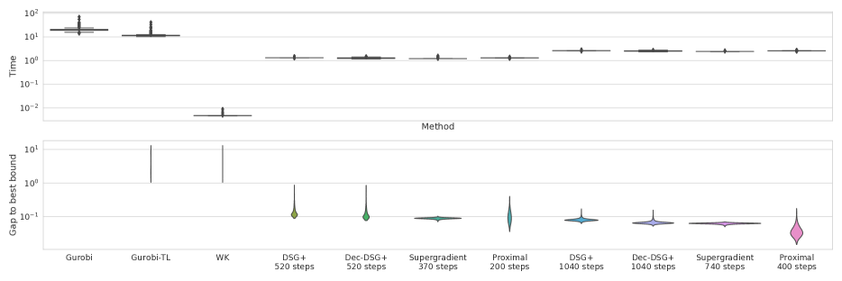
Figure 7: Comparison of the distribution of runtime and gap to optimality on a normally trained network. In both cases, lower is better. The width at a given value represents the proportion of problems for which this is the result. Note that Gurobi always return the optimal solution so doesn’t appear on the optimality gap, but is always the highest runtime.

Figures 7, 8, 9 show experiments (see section 6.3) for a network trained using standard stochastic gradient descent and cross entropy, with no robustness objective. We employ $\epsilon_{\text{verif}}=5/255$. Most observations done in the main paper for the adversarially trained network (Figures 2 and 3) still hold true: in particular, the advantage of the Lagrangian Decomposition based dual compared to the dual by Dvijotham et al., (2018) is even more marked than in Figure 3. In fact, for a subset of the properties, DSG+ has returns rather loose bounds even after $1040$ iterations. The proximal algorithm returns better bounds than the supergradient method in this case as well, even though the larger support of the optimality gap distribution and the larger runtime might reduce the advantages of the proximal algorithm.

Figure 8: Pointwise comparison for a subset of the methods in Figure 7. Each datapoint corresponds to a CIFAR image, darker colour shades mean higher point density. The dotted line corresponds to the equality and in both graphs, lower is better along both axes.

Figure 9: Additional pointwise comparison for a subset of the methods in Figure 7, along with the the omitted Interval Propagation (IP). Each datapoint corresponds to a CIFAR image, darker colour shades mean higher point density. The dotted line corresponds to the equality and in both graphs, lower is better along both axes.

G.1.1 Network Architecture

We now outline the network architecture for both the adversarially trained and the normally trained network experiments.

Conv2D(channels=16, kernel_size=4, stride=2)
Conv2D(channels=32, kernel_size=4, stride=2)
Linear(channels=100)
Linear(channels=10)

Table 2: Network architecture for incomplete verification, from Wong and Kolter, (2018). Each layer but the last is followed by a ReLU activation function.

G.2 Complete Verification

As done by Lu and Kumar, (2020), we provide a more in-depth analysis of the base model results presented in Figure 10. Depending on the time $t_{i}$ that the Gurobi baseline employed to verify them, the properties have been divided into an “easy” ($t_{i}<800$), “medium” and a “hard ” ($t_{i}>2400$) set. The relative performance of the iterative dual methods remains unvaried, with the initial gap between our two methods increasing with the difficulty of the problem.

Table 3: For easy, medium and difficult level verification properties on the base model, we compare average solving time, average number of solved sub-problems (on the properties that did not time out) and the percentage of timed out properties.

Easy Medium Hard Method time(s) sub-problems $\%$Timeout time(s) sub-problems $\%$Timeout time(s) sub-problems $\%$Timeout Gurobi-BaBSR $545.720$ $580.428$ $0.0$ $1370.395$ $1408.745$ $0.0$ $3127.995$ $2562.872$ $41.31$ MIPplanet $1499.375$ $16.48$ $2240.980$ $42.94$ $2250.624$ $46.24$ DSG+ BaBSR $112.100$ $2030.362$ $0.85$ $177.805$ $4274.811$ $0.52$ $1222.632$ $12\,444.449$ $23.71$ Supergradient BaBSR $85.004$ $1662.000$ $0.64$ $136.853$ $3772.679$ $0.26$ $1133.264$ $12\,821.481$ $21.36$ Proximal BaBSR $73.606$ $1377.666$ $0.42$ $129.537$ $3269.535$ $0.26$ $1126.856$ $12\,035.994$ $21.83$

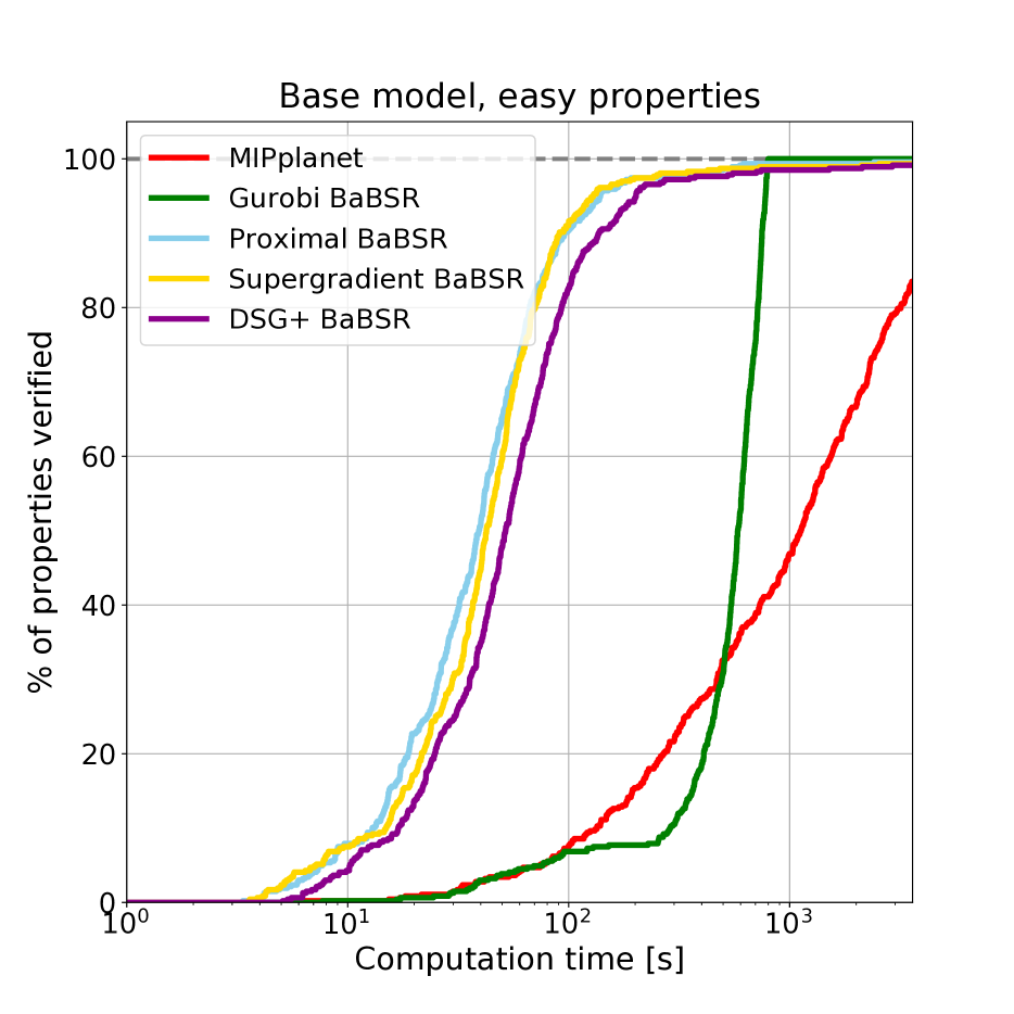
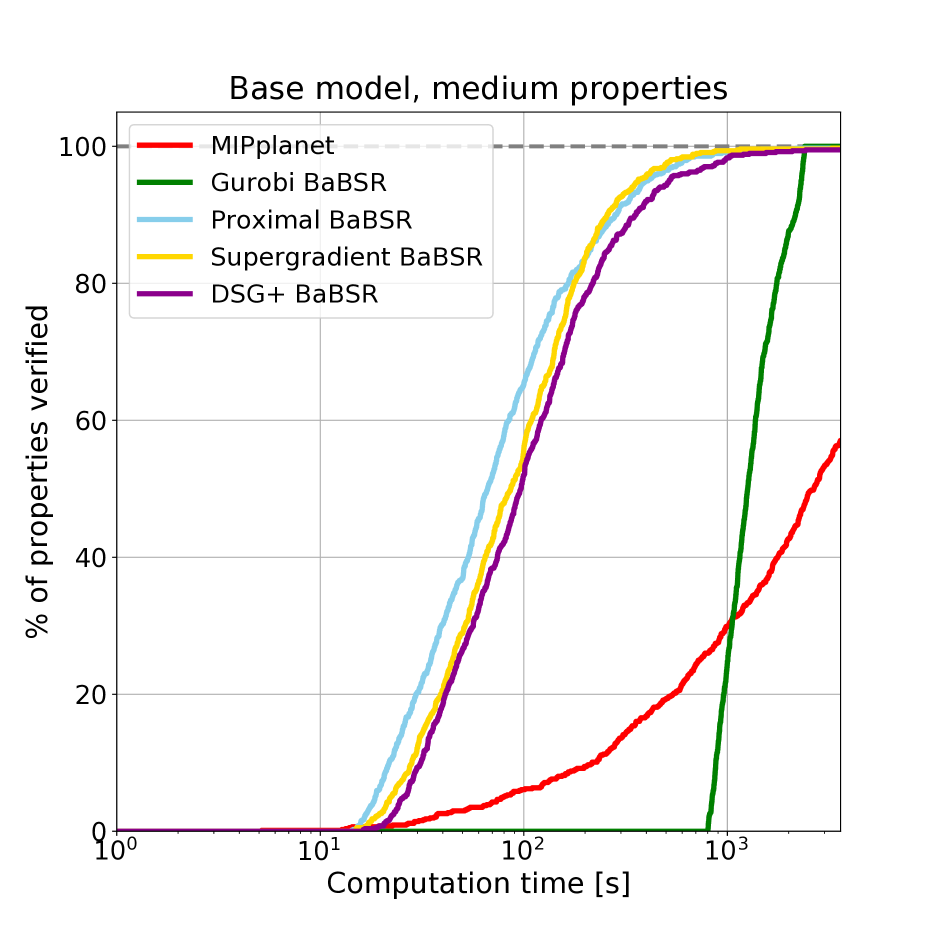
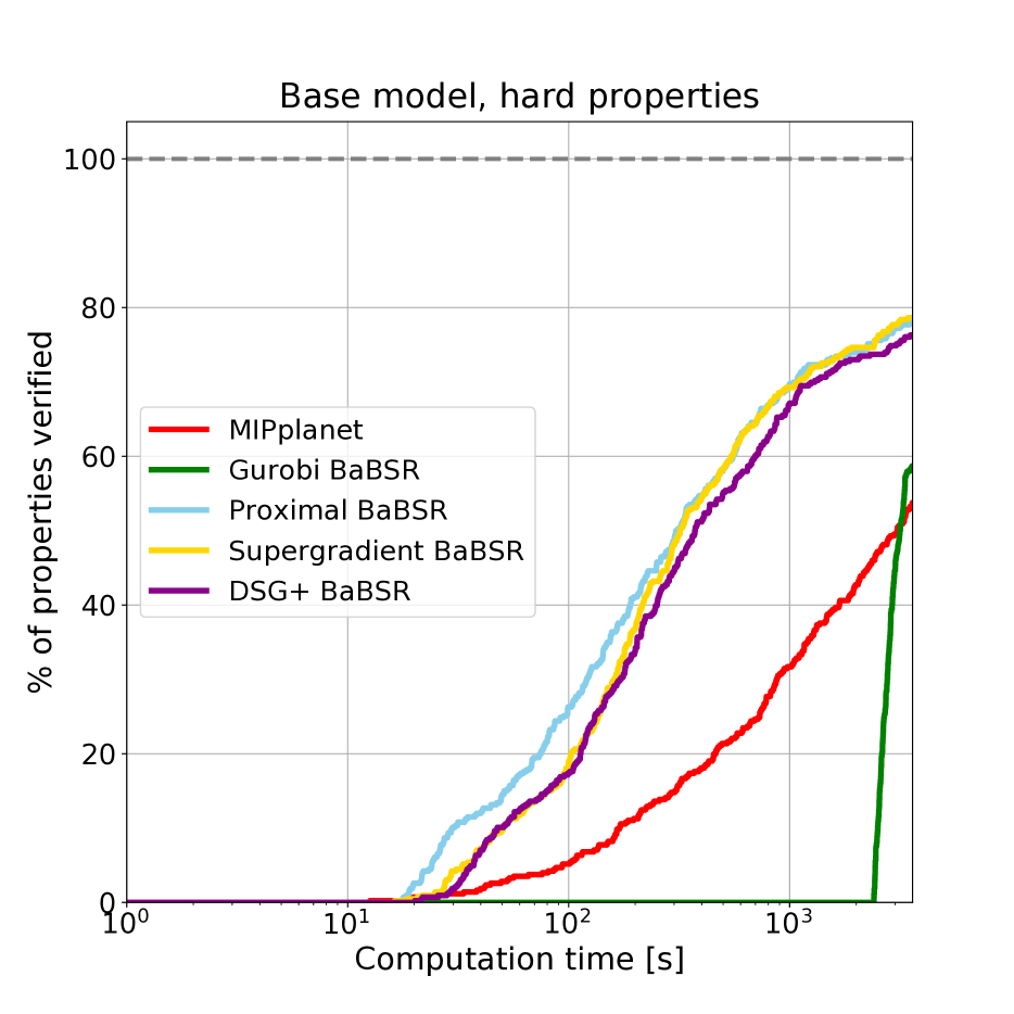
Figure 10: Cactus plots for the base model, with properties of varying difficulty. For each, we compare the bounding methods and complete verification algorithms by plotting the percentage of solved properties as a function of runtime.

G.2.1 Network Architectures

Finally, we describe properties and network architecture for the dataset by Lu and Kumar, (2020).

Network Name	No. of Properties	Network Architecture
BASE Model	Easy: 467 Medium: 773 Hard: 426	Conv2d(3,8,4, stride=2, padding=1) Conv2d(8,16,4, stride=2, padding=1) linear layer of 100 hidden units linear layer of 10 hidden units (Total ReLU activation units: 3172)
WIDE	300	Conv2d(3,16,4, stride=2, padding=1) Conv2d(16,32,4, stride=2, padding=1) linear layer of 100 hidden units linear layer of 10 hidden units (Total ReLU activation units: 6244)
DEEP	250	Conv2d(3,8,4, stride=2, padding=1) Conv2d(8,8,3, stride=1, padding=1) Conv2d(8,8,3, stride=1, padding=1) Conv2d(8,8,4, stride=2, padding=1) linear layer of 100 hidden units linear layer of 10 hidden units (Total ReLU activation units: 6756)

Table 4: For each complete verification experiment, the network architecture used and the number of verification properties tested, from the dataset by Lu and Kumar, (2020). Each layer but the last is followed by a ReLU activation function.

References

- Anderson et al., (2019) Anderson, R., Huchette, J., Tjandraatmadja, C., and Vielma, J. P. (2019). Strong mixed-integer programming formulations for trained neural networks. Conference on Integer Programming and Combinatorial Optimization.
- Athalye et al., (2018) Athalye, A., Carlini, N., and Wagner, D. A. (2018). Obfuscated gradients give a false sense of security: circumventing defenses to adversarial examples. International Conference on Machine Learning.
- Bach, (2015) Bach, F. (2015). Duality between subgradient and conditional gradient methods. SIAM Journal on Optimization.
- Bertsekas and Tsitsiklis, (1989) Bertsekas, D. P. and Tsitsiklis, J. N. (1989). Parallel and distributed computation: numerical methods. Prentice hall Englewood Cliffs, NJ.
- Bunel et al., (2020) Bunel, R., Lu, J., Turkaslan, I., Torr, P. H., Kohli, P., and Kumar, M. P. (2020). Branch and bound for piecewise linear neural network verification. Journal of Machine Learning Research.
- Bunel et al., (2018) Bunel, R., Turkaslan, I., Torr, P. H., Kohli, P., and Kumar, M. P. (2018). A unified view of piecewise linear neural network verification. Neural Information Processing Systems.
- Cheng et al., (2017) Cheng, C.-H., Nührenberg, G., and Ruess, H. (2017). Maximum resilience of artificial neural networks. Automated Technology for Verification and Analysis.
- Dvijotham et al., (2018) Dvijotham, K., Stanforth, R., Gowal, S., Mann, T., and Kohli, P. (2018). A dual approach to scalable verification of deep networks. Uncertainty in Artificial Intelligence.
- Ehlers, (2017) Ehlers, R. (2017). Formal verification of piece-wise linear feed-forward neural networks. Automated Technology for Verification and Analysis.
- Frank and Wolfe, (1956) Frank, M. and Wolfe, P. (1956). An algorithm for quadratic programming. Naval Research Logistics Quarterly.
- Goodfellow et al., (2015) Goodfellow, I. J., Shlens, J., and Szegedy, C. (2015). Explaining and harnessing adversarial examples. International Conference on Learning Representations.
- Gowal et al., (2018) Gowal, S., Dvijotham, K., Stanforth, R., Bunel, R., Qin, C., Uesato, J., Mann, T., and Kohli, P. (2018). On the effectiveness of interval bound propagation for training verifiably robust models. Workshop on Security in Machine Learning, NeurIPS.
- Guignard and Kim, (1987) Guignard, M. and Kim, S. (1987). Lagrangean decomposition: A model yielding stronger lagrangean bounds. Mathematical programming.
- Gurobi Optimization, (2020) Gurobi Optimization, L. (2020). Gurobi optimizer reference manual.
- Katz et al., (2017) Katz, G., Barrett, C., Dill, D., Julian, K., and Kochenderfer, M. (2017). Reluplex: An efficient smt solver for verifying deep neural networks. International Conference on Computer-Aided Verification.
- Kingma and Ba, (2015) Kingma, D. P. and Ba, J. (2015). Adam: A method for stochastic optimization. International Conference on Learning Representations.
- Lin et al., (2017) Lin, H., Mairal, J., and Harchaoui, Z. (2017). Catalyst acceleration for first-order convex optimization: From theory to practice. Journal of Machine Learning Research.
- Lu and Kumar, (2020) Lu, J. and Kumar, M. P. (2020). Neural network branching for neural network verification. In International Conference on Learning Representations.
- Madry et al., (2018) Madry, A., Makelov, A., Schmidt, L., Tsipras, D., and Vladu, A. (2018). Towards deep learning models resistant to adversarial attacks. International Conference on Learning Representations.
- Mirman et al., (2018) Mirman, M., Gehr, T., and Vechev, M. (2018). Differentiable abstract interpretation for provably robust neural networks. International Conference on Machine Learning.
- Paszke et al., (2017) Paszke, A., Gross, S., Chintala, S., Chanan, G., Yang, E., DeVito, Z., Lin, Z., Desmaison, A., Antiga, L., and Lerer, A. (2017). Automatic differentiation in pytorch. NIPS Autodiff Workshop.
- Raghunathan et al., (2018) Raghunathan, A., Steinhardt, J., and Liang, P. S. (2018). Semidefinite relaxations for certifying robustness to adversarial examples. Neural Information Processing Systems.
- Salman et al., (2019) Salman, H., Yang, G., Zhang, H., Hsieh, C.-J., and Zhang, P. (2019). A convex relaxation barrier to tight robustness verification of neural networks. Neural Information Processing Systems.
- Salzo and Villa, (2012) Salzo, S. and Villa, S. (2012). Inexact and accelerated proximal point algorithms. Journal of Convex Analysis, 19:1167–1192.
- Szegedy et al., (2014) Szegedy, C., Zaremba, W., Sutskever, I., Bruna, J., Erhan, D., Goodfellow, I., and Fergus, R. (2014). Intriguing properties of neural networks. International Conference on Learning Representations.
- Tjeng et al., (2019) Tjeng, V., Xiao, K., and Tedrake, R. (2019). Evaluating robustness of neural networks with mixed integer programming. International Conference on Learning Representations.
- Uesato et al., (2018) Uesato, J., O’Donoghue, B., Oord, A. v. d., and Kohli, P. (2018). Adversarial risk and the dangers of evaluating against weak attacks. International Conference on Machine Learning.
- Weng et al., (2018) Weng, T.-W., Zhang, H., Chen, H., Song, Z., Hsieh, C.-J., Boning, D., Dhillon, I. S., and Daniel, L. (2018). Towards fast computation of certified robustness for relu networks. International Conference on Machine Learning.
- Wong and Kolter, (2018) Wong, E. and Kolter, Z. (2018). Provable defenses against adversarial examples via the convex outer adversarial polytope. International Conference on Machine Learning.
- Xiang et al., (2017) Xiang, W., Tran, H.-D., and Johnson, T. T. (2017). Output reachable set estimation and verification for multi-layer neural networks. IEEE Transactions on Neural Networks and Learning Systems.