DeepPlume: Very High Resolution Real-Time Air Quality Mapping
Abstract.
This paper presents an engine able to predict jointly the real-time concentration of the main pollutants harming people’s health: nitrogen dioxyde (NO2), ozone (O3) and particulate matter (PM2.5 and PM10, which are respectively the particles whose size are below and ).
The engine covers a large part of the world and is fed with real-time official stations measures, atmospheric models’ forecasts, land cover data, road networks and traffic estimates to produce predictions with a very high resolution in the range of a few dozens of meters. This resolution makes the engine adapted to very innovative applications like street-level air quality mapping or air quality adjusted routing.
Plume Labs has deployed a similar prediction engine to build several products aiming at providing air quality data to individuals and businesses. For the sake of clarity and reproducibility, the engine presented here has been built specifically for this paper and differs quite significantly from the one used in Plume Labs’ products. A major difference is in the data sources feeding the engine: in particular, this prediction engine does not include mobile sensors measurements.
1. Introduction
Air pollution is one of the major public health concern. World Health Organization (WHO) estimates that more than 80% of citizens living in urban environments where air quality is monitored are exposed to air quality levels that exceed WHO guideline limits. It also estimates that million deaths every year are linked to outdoor air pollution (Organization, 2016).
Despite those alarming figures, very few citizens have access to information about the quality of the air they breathe. More and more public and private initiatives are being developed to close this gap and give to citizens the information they need to protect themselves from air pollution.
This is a particularly challenging topic because air quality varies a lot, both in time and in space. For example, a polluted air can clean itself in a few hours after a heavy rain. Also, a crowded street can be much more polluted than a green park area a few hundreds meters away (Monks et al., 2009).
One of the key difficulties when it comes to air quality modeling is the lack of data: it is believed that there are about thousands air quality monitoring stations worldwide, which is orders of magnitude below the number of stations needed given how much air quality varies in space. Also, there is as far as we know no comprehensive database providing the monitoring stations live and historical measurements, and building this database is a very time-consuming task.
The quantity of air quality data varies a lot depending on the location: urban areas in developed countries are generally well monitored, with dozens of monitoring stations in cities like London or Beijing. However, rural areas and poorer countries may be covered very sparsely given the high cost of building and maintaining an air quality monitoring network (the monitoring stations set up by public authorities cost generally between $10k and $50k per station).
This paper presents an engine able to predict the concentrations of atmospheric pollutants regulated by WHO: nitrogen dioxide (NO2), ozone (O3) and particulate matter (PM2.5 and PM10, which are respectively the particles whose size are below and ). The predictions are performed at a large scale covering whole countries or continents and with a high resolution in the range of a few dozens of meters.
Air quality depends highly on the region considered: for example, coal power plants produce a large part of air pollution in countries like China and India (Singh et al., 2019) while their impact is more limited in Western Europe. For this reason, we choose to estimate prediction models region per region. The geographical cover of the prediction engine is shown on Figure 1.
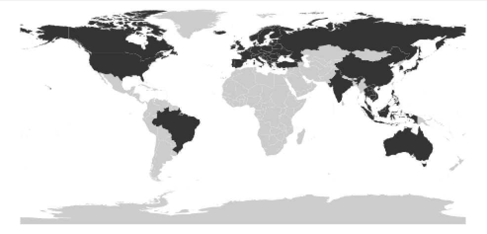
The regions covered by the prediction engine are displayed in black on this map.
The engine uses the air quality measurements provided by thousands of monitoring stations across the world, atmospheric simulations run by atmospheric science labs whose results are made available, and anthropogenic emissions estimates based on diverse datasets.
It is based on a somewhat classical neural network architecture, and tackles the data sparsity issue encountered in some regions with a transfer learning strategy: a global prediction model is learnt on a global dataset, and the final prediction layer is specialized on each regional dataset.
The paper is organized as follows. We discuss earlier works in Section 2. Section 3 gives a detailed overview of the data sources used, and describes how the features feeding the engine are built. Section 4 presents the structure of the prediction engine and details the model estimation process. Section 5 provides an evaluation of the prediction engine. Section 6 lists a few applications built on top of it.
2. Related work
The problem of air quality prediction is much studied in the literature and is tackled through various angles. (Ayturan et al., 2018) and (Kaur et al., 2017) present comprehensive reviews of air quality modeling using machine learning approaches.
Some papers focus on air quality temporal forecasts and aim at predicting pollutants concentration at air quality monitoring stations using the stations historical measurements and meteorological features. Most of them are based on neural networks (generally RNN or LSTM architectures) and the forecast horizon varies from a few hours to hours. (Reddy and Mohanty, 2017), (Fan et al., 2017) and (Huang and Kuo, 2018) build forecast models in China, (V et al., 2018) and (Rao et al., 2019) build models for indian cities.
Other papers propose spatiotemporal modeling frameworks. (Shuo and Gaoxiang, 2018) and (Wen et al., 2018) use Convolutional LSTM networks introduced in (Shi et al., 2015) for precipitation forecasting. The networks are fed with monitoring stations measurements and meteorological features to build 24 hours to 48 hours air quality forecasts. The spatial resolution in (Shuo and Gaoxiang, 2018) is degree. (Zhao et al., 2018), (Qi et al., 2017) and (Du et al., 2018) use similar deep learning architectures to build air quality forecasts in China. (Zhao et al., 2018) covers all China with a degree resolution, (Qi et al., 2017) covers Beijing with a kilometer resolution and (Wang and Song, 2018) focuses also on Beijing. (Yi et al., 2018) provides fine-grained forecasts in Chinese cities using a deep learning spatio-temporal architecture.
(Zheng et al., 2013) and (Zheng et al., 2015) propose different architectures mixing a spatial and a temporal predictor to build air quality forecasts in a few chinese cities with a kilometer resolution. Their approach uses additional features like traffic or land-use features.
Also, some papers introduce equations based on dispersion modeling in the prediction methodology in order to reduce overfitting due to the low number of monitoring stations available. (Ma et al., 2018) uses a hybrid architecture to build air quality maps in Tianjin, China, and (Fei et al., 2019) builds air quality forecasts in Chengdu, China.
(Shaddick et al., 2016) and (Sabath et al., 2018) focus on spatial air quality predictions. (Shaddick et al., 2016) builds global PM2.5 predictions based on monitoring stations and satellite-based measurements with a degree resolution using statistical modeling. (Sabath et al., 2018) models PM2.5 in the US using monitoring stations measurements, atmospheric models outputs and land-use datasets.
Finally, a few papers show how using mobile low-cost sensors networks can improve air quality predictions accuracy. (Apte et al., 2017) shows the results of experiments in Mountain View and San Francisco, (Marjovi et al., 2015) presents modeling approaches on an experimental setup in Lausanne, Switzerland, and (Song and Han, 2019) presents a case-study in Beijing using mobile sensors. These approaches are very promising but need expensive setups (deployment of mobile sensors networks) which can not be performed on a global scale.
3. Data sources and features
This section details the data sources used by the prediction engine and the features computation for each data source. The availability and reliability of those data sources vary from a region to the other and are a key factor of the engine’s overall accuracy.
We introduce the euclidean distance between two locations and . We define also the exponential kernel , where the distance is expressed in kilometers.
3.1. Air quality data
3.1.1. Monitoring stations measurements
We have built a proprietary architecture based on several dozens of crawlers collecting the air quality measurements provided by about monitoring stations across the world. Figure 2 shows a global map of the locations of those monitoring stations.
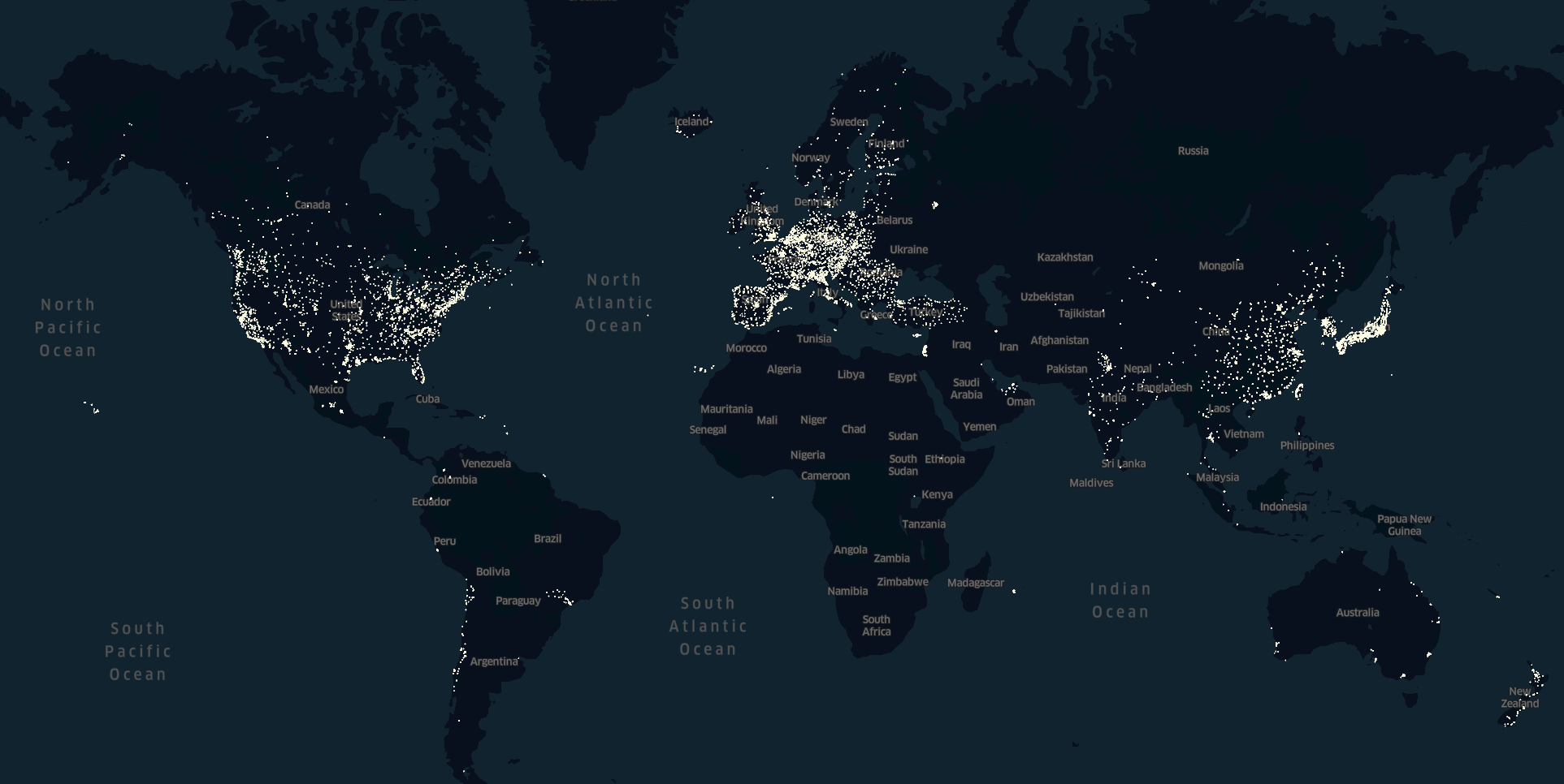
This map shows the locations of the monitoring stations whose air quality measurements feed the prediction engine.
Each monitoring station does not necessarily measure the four pollutants predicted by the engine. The resulting missing measurements have been flagged as in the datasets and are treated specifically. Table 1 gives the number of monitoring stations per region as well as the number of stations measuring each pollutant. As almost all monitoring stations give measurements on a hourly basis, the datasets have been built on a hourly basis.
| Region | Global | NO2 | O3 | PM2.5 | PM10 |
|---|---|---|---|---|---|
| Europe | 2778 | 2252 | 1614 | 790 | 1958 |
| United States | 1924 | 331 | 1300 | 1041 | 347 |
| Japan / S. Korea | 1924 | 1804 | 309 | 1345 | 313 |
| China | 1390 | 1385 | 1387 | 1387 | 1387 |
| Canada | 299 | 103 | 236 | 220 | 17 |
| Southeast Asia | 66 | 55 | 52 | 41 | 44 |
| India | 231 | 223 | 213 | 224 | 201 |
| Brazil | 51 | 39 | 41 | 20 | 46 |
| Australia | 66 | 42 | 34 | 47 | 54 |
| Russia | 29 | 20 | 15 | 15 | 21 |
We include in the datasets the measurements from January 1st, 2018 to December 31st, 2019. We have found that there are missing and erroneous values (generally abnormally high) coming from those monitoring stations. They can be encountered during station maintenance windows, during station failures or if issues arise during the publishing or collection of said data. While we are not able to determine the exact cause of such errors, it is important to detect them and define an appropriate treatment: missing values are discarded from the datasets, and erroneous values are detected using an outlier detection engine and then discarded.
For any distance and for each pollutant , we define the feature at every location as the weighted average of the monitoring stations measurements for pollutant at time . We define also as the sum of the weights. The weights are computed with an exponential kernel .
can be interpreted as a predictor of the concentration of pollutant based on the measurements of the monitoring stations around. measures the density of monitoring stations and can be interpreted as a level of confidence in : the more monitoring stations there are around a point, the more robust the weighted average measure is.
3.1.2. Mobile sensors data
While stations measurements provide useful ground-truth values for air quality modeling, such data sources are constrained by two limits:
-
•
Data sparsity: because monitoring stations are expensive to build and maintain, large areas are not or sparsely covered, including in densely populated areas
-
•
Data delay: there is often a significant delay between the time a measurement is made and the time this measurement is made available. This delay can be as high as a few hours, thus decreasing the relevance of the measurement for live monitoring and forecasts
Mobile low-cost sensors provide an abundant source of data, and unlike fixed stations which monitor a single location, they are able to map a larger area. We therefore believe that those sensors are a valuable and useful complement to standard monitoring stations. To that end, Plume Labs has developed Flow111https://plumelabs.com/en/flow/, a personal wearable air quality sensor that measures NO2, VOCs, PM10, PM2.5 and PM1 on a minute-by-minute basis. This sensor being cheaper and easier to maintain than typical monitoring stations, it can be deployed in ad-hoc sensing networks over selected regions to provide prediction engines with valuable ground-truth data.
The use of both fixed stations and low-cost mobile sensors measurements in the prediction engine is a particularly challenging area of research. Gaussian process regression provides a natual theoretical framework to aggregate both sources of data in a consistent way, taking into account the different accuracy of the measurements coming from fixed stations and low-cost sensors.
3.1.3. Atmospheric models simulations
Atmospheric models rely on physical and chemical modeling of pollutants’ emissions and dispersion, and the simulations are initiated with monitoring stations and satellite-based measurements. Each atmospheric model is characterized by its geographical cover (regional or global) and its spatial granularity (generally a few dozens of kilometers).
We define the feature at every location by doing a bilinear interpolation of the forecasts at time produced on the grid for pollutant by the atmospheric model with the best resolution around .
It is worth noting that those simulations have a poor spatial granularity compared to the resolution reached by our engine. However, they provide a very valuable input in regions which are not or sparsely covered with monitoring stations, typically outside urban areas.
3.2. Anthropogenic emissions datasets
3.2.1. Traffic data
We collect traffic data through a real-time jam factor over each road segment of a given area. The jam factor is a value between and measuring the road congestion: means that the road is not congested while means that it is very congested. Historical and real-time traffic data are collected across Europe and the United States.
For any distance , we define the feature at every location as the weighted sum of the jam factors of the road segments around location , and each road segment is weighted by the product of its length and its functional class222The functional class is a classification of each road segment, from 1 (meaning a small road) to 5 (meaning a large road).. The weights are computed with the exponential kernel .
The product of the jam factor, the length and the functional class on a road segment is supposed to be proportional to the traffic emissions on this road segment. Hence, this feature can be interpreted as a proxy of traffic emissions around.
3.2.2. Road networks
We have road network details and topology in the regions covered by the prediction engine. Road network data is collected as a set of road segments, and any road segment is associated with a set of metadata regrouping a significant number of informations including a classification per usage, e.g., motorway or residential. We have built two aggregate categories named Roads and MajorRoads.
We define the features and for every location as the weighted length of roads and major roads around location , the weights being computed with an exponential kernel . Those features estimate the roads density around a location , and can be interpreted as a rough proxy of the number of vehicles around.
3.2.3. Land-use data
Land-use datasets (also called land cover datasets), classify the land into several categories like residential areas or green areas. Different datasets have been used, each characterized by its geographical cover, its spatial resolution and the granularity of the categories provided. We have built three aggregate categories named Industry, Residential and Green.
For each category, we define the corresponding feature for a distance at every location as the weighted share of land flagged with the category. The weights are computed with the exponential kernel .
3.2.4. Power plants emissions
Electrical power plants, and in particular coal power plants are a major source of air pollution in some regions. A global power plant database giving the location, maximum capacity and type (coal, gas or oil) of all power plants is used to build an estimation of the resulting pollution emissions.
4. Model estimation
The prediction engine maps the features with the 4-dimensional vector giving the pollutants concentrations in using a classical neural network with hidden layers of sizes and . We use rectified linear activation functions in the inner layers of the network, and the identity function in the output layer.
4.1. Datasets’ description
In each region, we have built a dataset containing the monitoring stations measurements as well as the features used by the prediction engine. Each data point corresponds to the measurements returned by an air quality monitoring station at a given time. The time range covers a period from January 1st, 2018 to December 31st, 2019. We have considered for each feature different distances from meters to kilometers. Missing measurements are flagged as : most of the time, it is because the monitoring station does not monitor the pollutant considered. The datasets have been built in Python using various packages including Scikit-Learn and Numpy. Table 2 gives the total number of data points in each region.
It is worth noting that for each data point, the corresponding monitoring station is excluded from the monitoring stations used to build the features and , to make sure that the measurements on which the predictor is trained are not included in the features.
| Region | Number of data points |
|---|---|
| Europe | 36.2 mlns |
| United States | 26.9 mlns |
| Japan / S. Korea | 29.0 mlns |
| China | 18.9 mlns |
| Canada | 4.29 mlns |
| Southeast Asia | 0.88 mlns |
| India | 0.82 mlns |
| Brazil | 0.67 mlns |
| Australia | 0.61 mlns |
| Russia | 0.27 mlns |
4.2. Estimation setup
In each region, the set of monitoring stations is splitted randomly into two parts: of the stations are used to build the training dataset and the remaining are used to build the evaluation dataset. This method ensures that the evaluation is performed at locations which are not included at all during the training.
Then, the training and evaluation datasets are built by sampling the data points the following way:
-
•
Plume Labs internal Air Quality Index333An Air Quality Index (AQIs) is a normalization of a pollutant raw concentration in to a health impact scale, allowing inter-pollutant comparison. AQIs are commonly used worldwide and are usually defined locally at the country or continent scale to comply with local standards. Plume Labs AQI is based on WHO recommendations and is extensively described here: https://plumelabs.zendesk.com/hc/en-us/articles/360008268434-What-is-the-Plume-AQI-. A global AQI value can be calculated as the maximum of single pollutants’ AQIs. (PAQI) (see (Leonardi and Quennehen, 2016)) is computed for each data point (using the pollutants with non-missing measurements only), and is used to split the datasets into parts depending on the corresponding air pollution exposure: Low, Moderate, High and Very High
-
•
For each region, the same number of data points are sampled with replacement in each exposure category. In the experiments detailed in this paper, we have sampled million points in each exposure category to build the training dataset, and thousand points in each exposure category to build the evaluation dataset. Consequently, for each region, the size of the training dataset is million points, and the size of the evaluation dataset is thousand points
This sampling ensures that the prediction engine remains accurate for all air quality levels, while using the raw datasets leads to a better accuracy for good air quality levels at the cost of a worse accuracy when pollution levels are high, because low pollutants concentrations are more frequent in the datasets.
Then, the models are trained on the training datasets using TensorFlow and Keras. The loss used in training is the mean squared logarithmic error (MSLE) loss. values are excluded of the loss computation. We use Adam optimizer with a learning rate equal to . The batch size is . In Europe and in the United States, the prediction models are estimated on the Europe and United States datasets respectively. In the other regions, we use a transfer learning strategy described below.
4.3. Transfer learning strategy in regions with few data
In some regions where there are few monitoring stations, the prediction model trained using the monitoring stations located in the region only was not robust enough. We use the following transfer learning strategy, summarized on Figure 3:
-
•
First, a global model is learnt on a global dataset built by concatenating the datasets of all the regions. This phase corresponds to the left network on Figure 3
-
•
Then, the final prediction layer of the global model is trained on the regional dataset. This phase corresponds to the right network on Figure 3
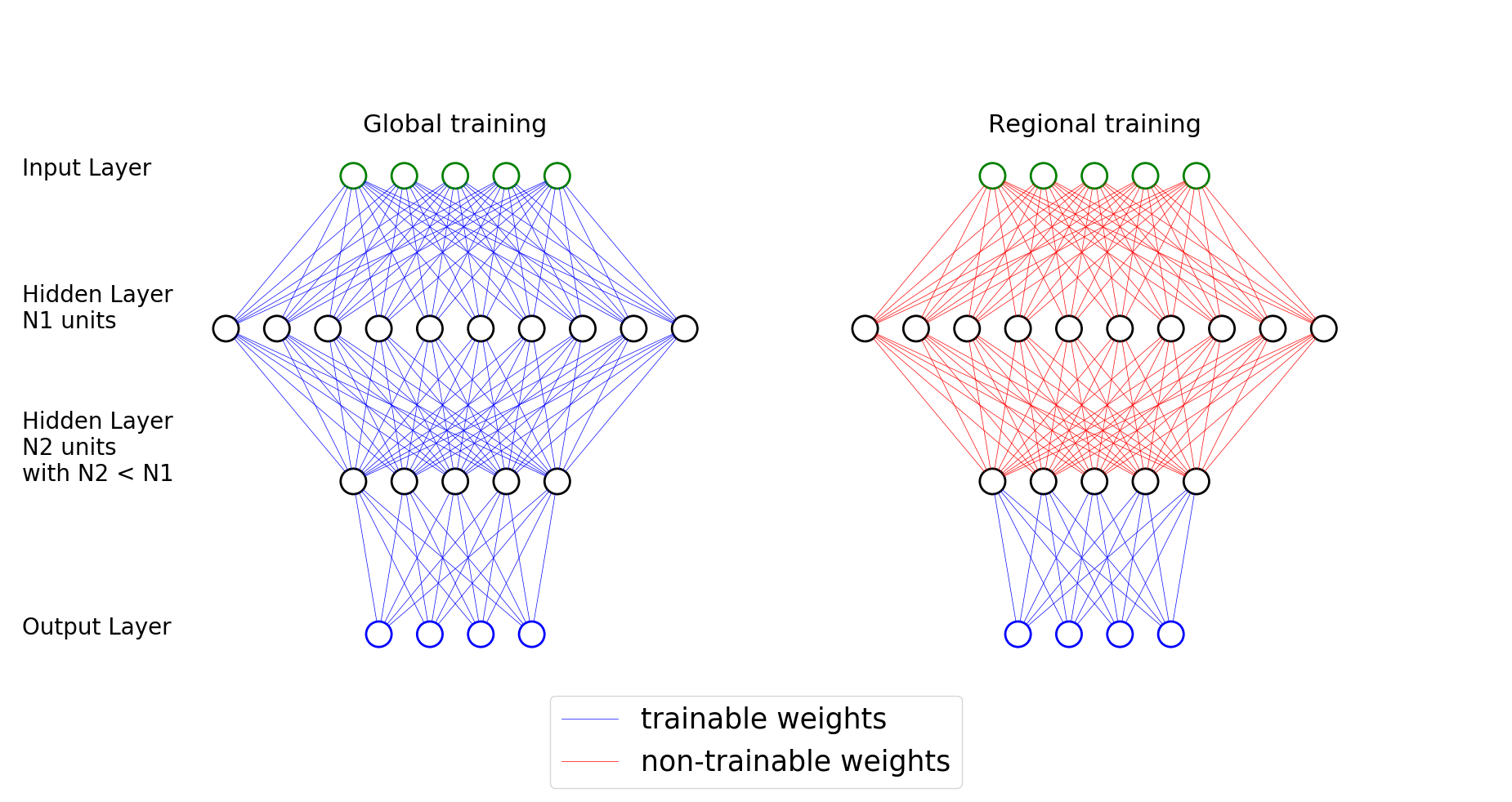
This diagram highlights the transfer learning strategy applied in regions with few data.
This strategy has been applied in the regions where the datasets contain less than million data points: this threshold has been determined empirically. The next section shows how it improves the predictions accuracy in those regions.
4.4. Features selection
The results presented in this paper are based on a prediction model using a subset of the features described in Section 3. In particular, mobile sensors measurements are not integrated. Table 3 summarizes the features used by the prediction engine in each region.
| Region | Features |
|---|---|
| Europe, United States | for all pollutants, |
| for all pollutants, | |
| for all pollutants, | |
| for all pollutants, | |
| for all pollutants, | |
| , , , | |
| , , | |
| Other regions | for all pollutants, |
| for all pollutants, | |
| for all pollutants, | |
| , | |
| for all pollutants | |
| , , | |
| , |
We can give the following interpretations for the features selected:
-
•
The features can be interpreted as an estimate of air quality based on the monitoring stations around. The distances , and kilometers have been selected: is a good predictor in areas with many monitoring stations while higher distances ( and ) are more relevant when the monitoring stations are sparsely located. Using distances higher than kilometers did not improve the accuracy of the predictions
-
•
The counters provide a proxy of the surrounding stations’ density, which can be interpreted as the robustness of the weighted average of the stations measurements. Adding the counters computed with other distances did not bring additional predictive power at the cost of adding several features: that is why one distance only is used
-
•
The feature based on the atmospheric models forecasts can be interpreted as a background air quality level and adds predictive power in regions with few monitoring stations
-
•
The features modeling the impact of human activity (land cover, roads network and traffic) are built with a much smaller distance ( meters) which brings much more predictive power than higher distances
5. Model evaluation
5.1. Prediction model evaluation
The prediction models estimated for each region are compared to a benchmark predictor which consists in predicting for each pollutant the measure provided by the closest monitoring station. The evaluation metric is the MSLE loss function used to train the models. Table 4 compares the metric computed for the prediction model and the benchmark predictor on the evaluation dataset for each region. The model brings a very significant MSLE decrease in all regions compared to the benchmark predictor.
| Region | Benchmark | Prediction model | Improvement (in %) |
|---|---|---|---|
| Europe | 0.355 | 0.184 | -48.2 |
| United States | 0.461 | 0.318 | -31.0 |
| Japan / S. Korea | 0.233 | 0.14 | -39.9 |
| China | 0.317 | 0.214 | -32.5 |
| Canada | 0.441 | 0.392 | -11.1 |
| Southeast Asia | 1.234 | 0.901 | -27.0 |
| India | 0.698 | 0.351 | -49.7 |
| Brazil | 0.442 | 0.318 | -28.1 |
| Australia | 0.355 | 0.305 | -14.1 |
| Russia | 0.541 | 0.387 | -28.5 |
Europe is the region with the most monitoring stations and consequently the biggest dataset. On Europe evaluation dataset we present a more detailed evaluation:
-
•
Table 5 gives the MSLE computed for each pollutant for the prediction model and the benchmark predictor. It shows that the prediction model performs significantly better than the benchmark predictor for every pollutant
-
•
Figure 4 displays for each pollutant the measure and the concentration predicted by the prediction model or the benchmark predictor on the evaluation dataset. The predictions obtained with the prediction model are clearly much closer to the actual measurements than the ones produced by the benchmark predictor
| Pollutant | Benchmark | Prediction model | Improvement (in %) |
|---|---|---|---|
| NO2 | 0.530 | 0.230 | -56.6 |
| O3 | 0.330 | 0.215 | -34.8 |
| PM2.5 | 0.289 | 0.154 | -46.7 |
| PM10 | 0.271 | 0.139 | -48.7 |
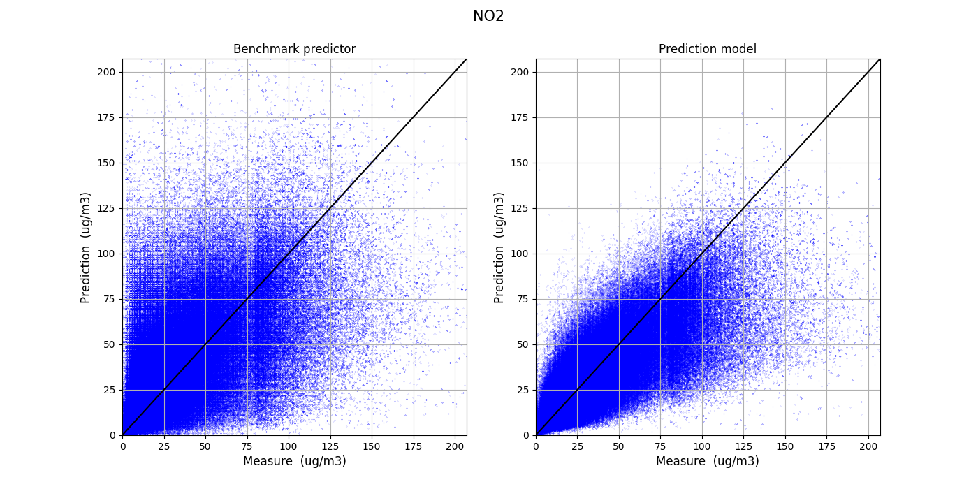
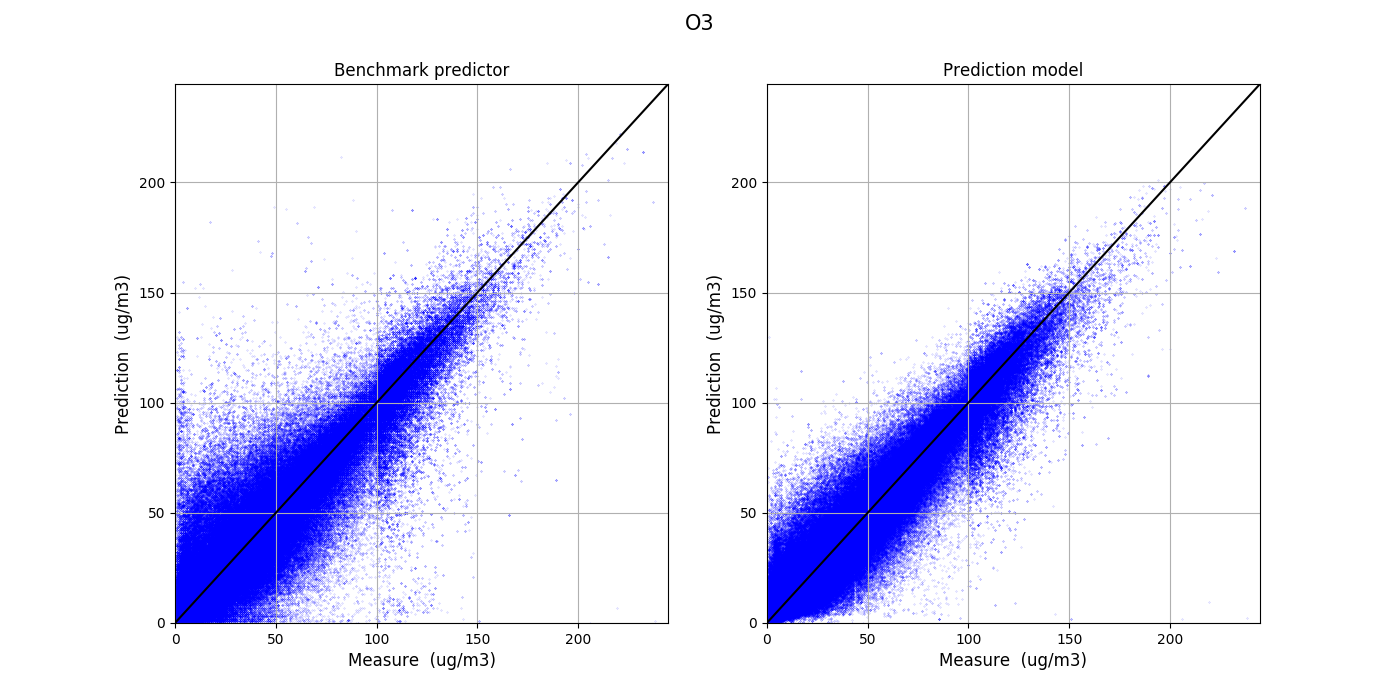
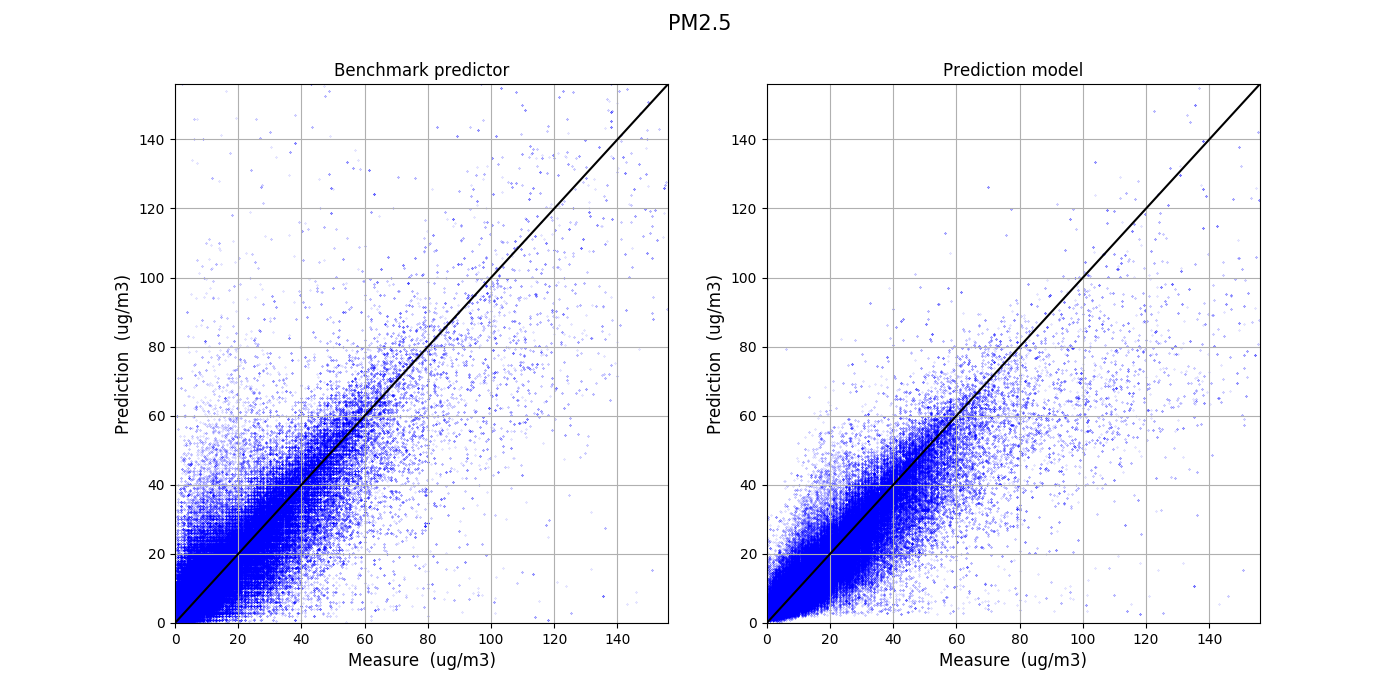
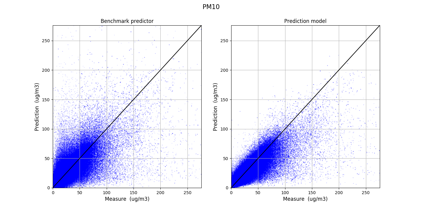
For each pollutant, these plots show the air quality measurements (X axis) and the predictions obtained by the benchmark predictor (Y axis, left plot) or the prediction model (Y axis, right plot)
5.2. Evaluation of the transfer learning strategy
In the regions where transfer learning is used to estimate the prediction models, we compare the accuracy of the three following models: the model trained on the global training dataset (Global), the model trained on the regional training dataset only (Regional), and the model trained using the transfer learning approach (Transfer learning). Table 6 compares the evaluation metric computed on each region’s evaluation dataset with those models. In all regions excluding Brazil, the model estimated using transfer learning performs better than both the model estimated on the global dataset and the model estimated on the regional dataset.
| Region | Global | Regional | Transfer learning |
|---|---|---|---|
| Southeast Asia | 1.000 | 1.070 | 0.901 |
| India | 0.375 | 0.508 | 0.351 |
| Brazil | 0.332 | 0.298 | 0.318 |
| Australia | 0.311 | 0.434 | 0.305 |
| Russia | 0.396 | 0.466 | 0.387 |
5.3. Features analysis
In this section, we analyze how each feature impacts the model prediction by building a partial dependence plot for each feature. The partial dependence plot shows, for each value of a given feature, the average prediction if the feature is set at this value for all the data points. We have used this method because its results are particularly simple to understand. It is worth to keep in mind its limitations, in particular when the features are correlated, which is obviously the case here.
Figure 5 shows the partial dependence plots built for some features using Europe prediction model. Traffic, Roads and MajorRoads features have a high impact on the predictions: higher values are linked to an increase in concentrations for NO2, PM2.5 and PM10 and to a decrease in O3 concentration, which is the expected behaviour as the chemical interaction between NO2 and O3 make them unable to co-exist. The green feature has a more limited impact and a higher value is linked to an increase of O3 and to a decrease in NO2: this is, again, an expected behaviour as NO2 sources are highly related to car exhausts and residential heating.
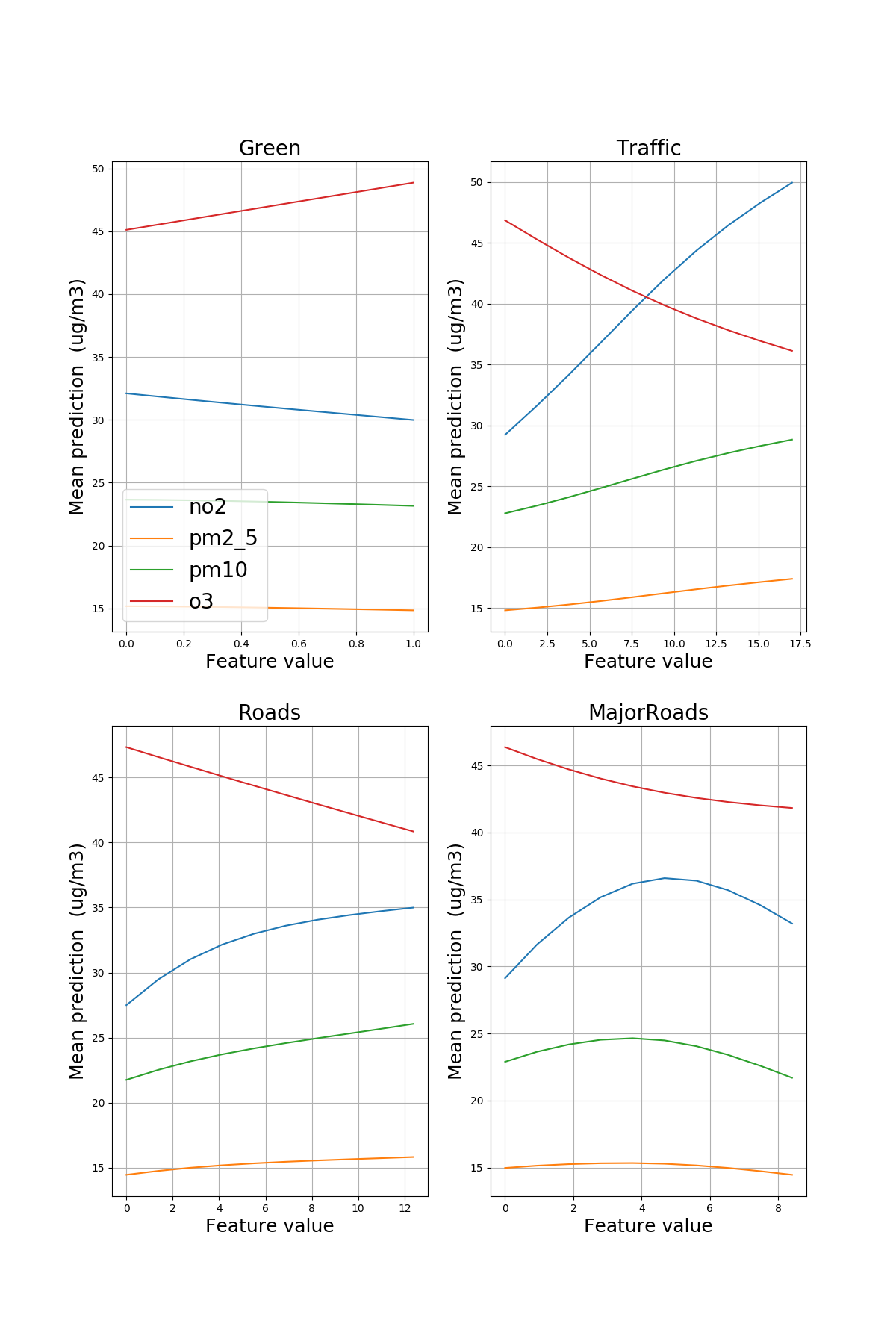
Partial dependence plot for some features in Europe
6. Applications
We describe here three applications made possible by this prediction engine: city-level street-level air quality mapping, air quality adjusted routing and large-scale air quality mapping.
6.1. Street-level air quality mapping
The prediction engine is used to build real-time street-level air quality maps in the world’s largest cities such as the one shown on Figure 6. This map has been built by applying the prediction engine at every road segment in the city.
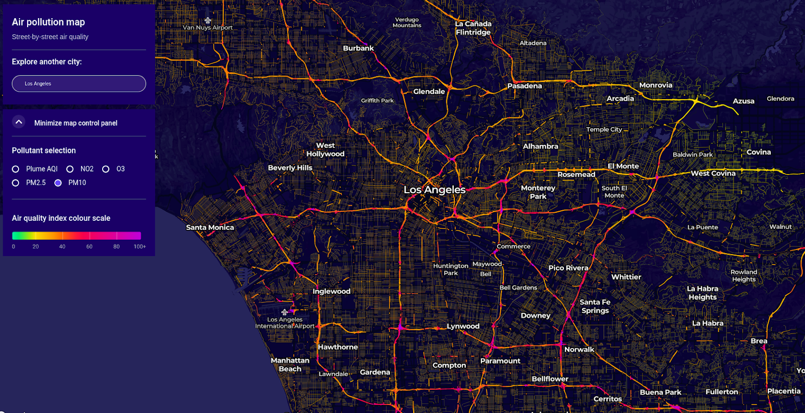
Street-level air quality map in Los Angeles
6.2. Air quality adjusted routing
In a city where street-level air quality mapping has been performed, we can build a routing engine for pedestrians which proposes several paths: the shortest one (what is returned by classical routing engines), but also alternative paths which may be longer but with a lower air pollution exposure.
Figure 7 shows an illustration of this routing engine in Paris. The shortest path is obtained by applying a classical shortest path algorithm on the road network where each road segment is weighted by its length. The alternative path is obtained by weighting each road segment by the product of its length and its predicted Plume AQI. In this example, the alternative path is longer but less polluted.
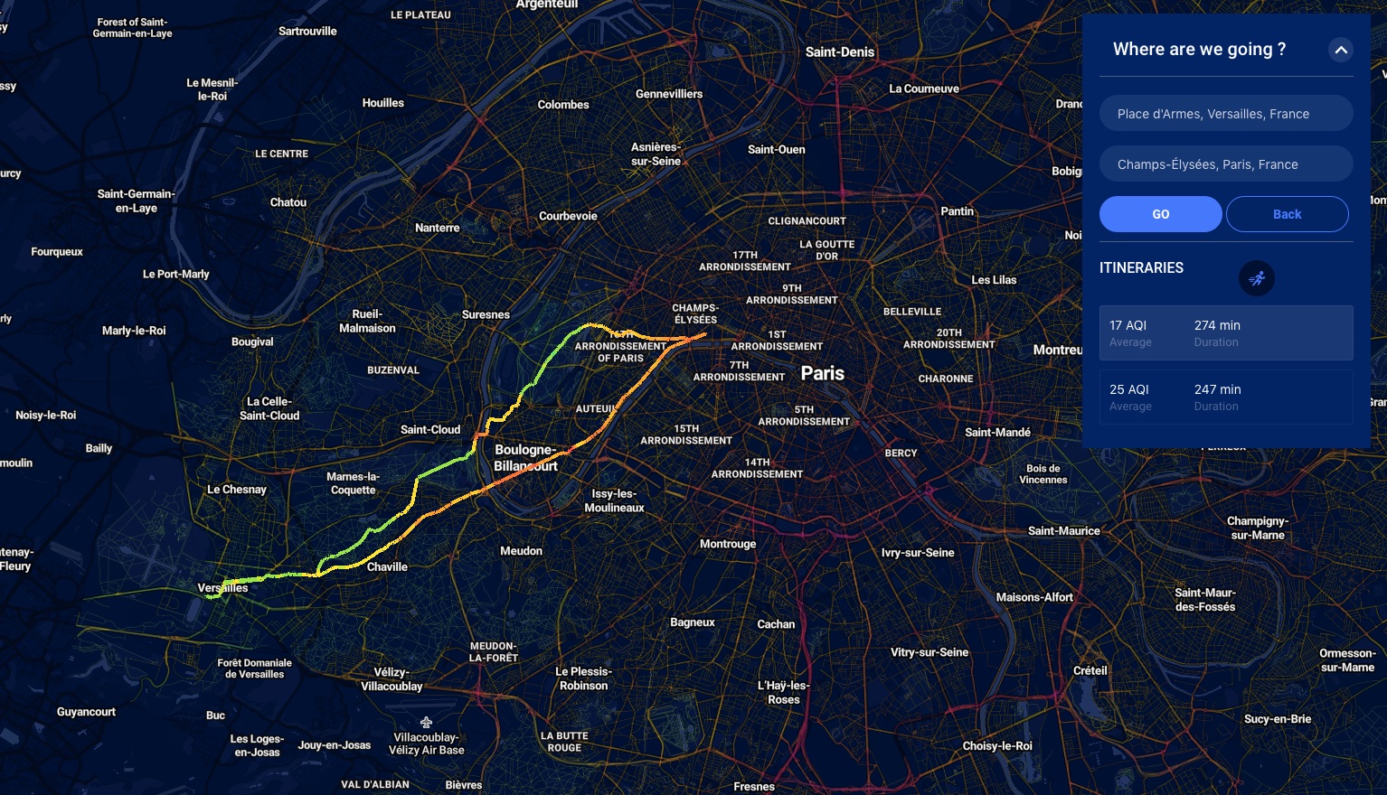
Air quality adjusted routing in Paris
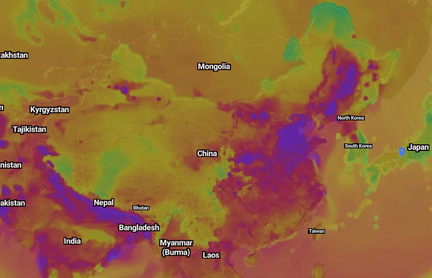
6.3. Large-scale air quality mapping
The prediction engine can also be used to build large-scale air quality heatmaps like the one shown on Figure 8. It is worth noting that global air pollution visualizations must be presented using a global air quality index: we choose Plume AQI (presented in (Leonardi and Quennehen, 2016)) which is as far as we know the only one available.
7. Conclusion and future work
The engine presented in this paper is at our knowledge the first modeling framework covering such a large part of the world with a resolution of a few dozens of meters. Indeed, most of existing works focus on a paticular city or country with a resolution higher than kilometer. Reaching such a fine resolution is needed to produce accurate air quality mappings given the high spatial variability of air quality, and enables to build innovative applications that individuals can use to protect themselves from air pollution, like air quality adjusted routing.
A scope for improvement is on how the features feeding the engine are built. In the work described here, they are computed using an isotropic exponential kernel. Defining other types of kernels, and in particular non-isotropic ones, would lead to a better modeling of spatial correlations. The kernels could also be learnt in the way they are learnt in a convolutional neural network, but this would make more difficult to reach a very fine resolution on large regions. Defining and precomputing fixed kernel functions is what enabled us to reach such a high resolution compared to other state-of-the-art papers using convolutional neural networks.
The integration of mobile sensors measurements in an air quality prediction engine is particularly challenging, and we belive that it brings a very significant improvement in the predictions accuracy. These results will be presented in a future paper focused on this topic.
Finally, this paper studies the air quality spatial variability only and can be used to perform real-time air quality mapping. A logical improvement of the engine would be to integrate temporal variability as well to be able to provide temporal forecasts. This makes the prediction problem much more complex and more hardly compatible with the fine resolution reached here.
References
- (1)
- Apte et al. (2017) Joshua Apte, Kyle Messier, Shahzad Gani, Michael Brauer, Thomas Kirchstetter, Melissa Lunden, Julian Marshall, Christopher Portier, Roel Vermeulen, and Steven Hamburg. 2017. High-Resolution Air Pollution Mapping with Google Street View Cars: Exploiting Big Data. Environmental Science Technology 51 (06 2017). https://doi.org/10.1021/acs.est.7b00891
- Ayturan et al. (2018) Akın Ayturan, Zeynep Ayturan, and Hüseyin Altun. 2018. Air Pollution Modelling with Deep Learning: A Review. 1 (09 2018), 58–62.
- Du et al. (2018) Shengdong Du, Tianrui Li, Yan Yang, and Shi-Jinn Horng. 2018. Deep Air Quality Forecasting Using Hybrid Deep Learning Framework.
- Fan et al. (2017) J. Fan, Q. Li, J. Hou, X. Feng, Hamed Karimian, and S. Lin. 2017. A Spatiotemporal Prediction Framework for Air Pollution Based on Deep RNN. ISPRS Annals of Photogrammetry, Remote Sensing and Spatial Information Sciences IV-4/W2 (10 2017), 15–22. https://doi.org/10.5194/isprs-annals-IV-4-W2-15-2017
- Fei et al. (2019) Haolin Fei, Xiaofeng Wu, and Chunbo Luo. 2019. A Model-driven and Data-driven Fusion Framework for Accurate Air Quality Prediction.
- Huang and Kuo (2018) Chiou-Jye Huang and Ping-Huan Kuo. 2018. A Deep CNN-LSTM Model for Particulate Matter (PM2.5) Forecasting in Smart Cities. Sensors 18 (07 2018), 2220. https://doi.org/10.3390/s18072220
- Kaur et al. (2017) Gaganjot Kaur, Jerry Gao, Sen Chiao, Shengqiang Lu, and Gang Xie. 2017. Air Quality Prediction: Big data and Machine Learning Approaches.
- Leonardi and Quennehen (2016) Alexandre Leonardi and Boris Quennehen. 2016. Plume AQI: An Air Quality Index aligned with health recommendations. (2016).
- Ma et al. (2018) Rui Ma, Xiangxiang Xu, Yue Wang, Hae Noh, Pei Zhang, and Lin Zhang. 2018. Guiding the Data Learning Process with Physical Model in Air Pollution Inference. 4475–4483. https://doi.org/10.1109/BigData.2018.8622381
- Marjovi et al. (2015) Ali Marjovi, Adrian Arfire, and A. Martinoli. 2015. High Resolution Air Pollution Maps in Urban Environments Using Mobile Sensor Networks. 11–20. https://doi.org/10.1109/DCOSS.2015.32
- Monks et al. (2009) P.S. Monks, C. Granier, S. Fuzzi, A. Stohl, M.L. Williams, H. Akimoto, M. Amann, A. Baklanov, U. Baltensperger, I. Bey, N. Blake, R.S. Blake, K. Carslaw, O.R. Cooper, F. Dentener, D. Fowler, E. Fragkou, G.J. Frost, S. Generoso, P. Ginoux, V. Grewe, A. Guenther, H.C. Hansson, S. Henne, J. Hjorth, A. Hofzumahaus, H. Huntrieser, I.S.A. Isaksen, M.E. Jenkin, J. Kaiser, M. Kanakidou, Z. Klimont, M. Kulmala, P. Laj, M.G. Lawrence, J.D. Lee, C. Liousse, M. Maione, G. McFiggans, A. Metzger, A. Mieville, N. Moussiopoulos, J.J. Orlando, C.D. O’Dowd, P.I. Palmer, D.D. Parrish, A. Petzold, U. Platt, U. Pöschl, A.S.H. Prévôt, C.E. Reeves, S. Reimann, Y. Rudich, K. Sellegri, R. Steinbrecher, D. Simpson, H. ten Brink, J. Theloke, G.R. van der Werf, R. Vautard, V. Vestreng, Ch. Vlachokostas, and R. von Glasow. 2009. Atmospheric composition change – global and regional air quality. Atmospheric Environment 43, 33 (2009), 5268 – 5350. https://doi.org/10.1016/j.atmosenv.2009.08.021 ACCENT Synthesis.
- Organization (2016) World Health Organization. 2016. Ambient air pollution: a global assessment of exposure and burden of disease. World Health Organization. 121 p. pages.
- Qi et al. (2017) Zhongang Qi, Tianchun Wang, Guojie Song, Weisong Hu, Xi Li, Zhongfei, and Zhang. 2017. Deep Air Learning: Interpolation, Prediction, and Feature Analysis of Fine-grained Air Quality. IEEE Transactions on Knowledge and Data Engineering PP (11 2017). https://doi.org/10.1109/TKDE.2018.2823740
- Rao et al. (2019) K. Rao, G. Devi, and Narendra Ramesh. 2019. Air Quality Prediction in Visakhapatnam with LSTM based Recurrent Neural Networks. International Journal of Intelligent Systems and Applications 11 (02 2019), 18–24. https://doi.org/10.5815/ijisa.2019.02.03
- Reddy and Mohanty (2017) Vikram Narasimha Reddy and Shrestha Mohanty. 2017. Deep Air : Forecasting Air Pollution in Beijing , China.
- Sabath et al. (2018) M. Sabath, Qian Di, Danielle Braun, Francesca Dominici, and Christine Choirat. 2018. aipred: A Flexible R Package Implementing Methods for Predicting Air Pollution.
- Shaddick et al. (2016) Gavin Shaddick, Matthew Thomas, Amelia Jobling, Michael Brauer, Aaron Donkelaar, Rick Burnett, Howard Chang, Aaron Cohen, Rita Van Dingenen, Carlos Dora, Sophie Gumy, Yang Liu, Randall Martin, Lance Waller, Jason West, James Zidek, and Annette Prüss-Ustün. 2016. Data Integration Model for Air Quality: A Hierarchical Approach to the Global Estimation of Exposures to Ambient Air Pollution. Journal of the Royal Statistical Society. Series C: Applied Statistics (09 2016). https://doi.org/10.1111/rssc.12227
- Shi et al. (2015) Xingjian Shi, Zhourong Chen, Hao Wang, Dit-Yan Yeung, Wai Kin Wong, and Wang-chun WOO. 2015. Convolutional LSTM Network: A Machine Learning Approach for Precipitation Nowcasting. (06 2015).
- Shuo and Gaoxiang (2018) Sun Shuo and Liu Gaoxiang. 2018. Air Quality Forecasting Using Convolutional LSTM. (2018).
- Singh et al. (2019) Gyanesh Kumar Singh, Pradhi Rajeev, Debajyoti Paul, and Tarun Gupta. 2019. Atmospheric Emissions from Thermal (Coal-Fired) Power Plants and Associated Environmental Impacts. Springer Singapore, Singapore, 53–72. https://doi.org/10.1007/978-981-13-3281-4_4
- Song and Han (2019) Jun Song and Ke Han. 2019. Exploring Urban Air Quality with MAPS: Mobile Air Pollution Sensing.
- V et al. (2018) Athira V, Dr.geetha Srikanth, Vinayakumar R, and Soman Kp. 2018. DeepAirNet: Applying Recurrent Networks for Air Quality Prediction. Procedia Computer Science 132 (01 2018), 1394–1403. https://doi.org/10.1016/j.procs.2018.05.068
- Wang and Song (2018) Junshan Wang and Guojie Song. 2018. A Deep Spatial-Temporal Ensemble Model for Air Quality Prediction. Neurocomputing 314 (06 2018). https://doi.org/10.1016/j.neucom.2018.06.049
- Wen et al. (2018) Cc Wen, Liu Shufu, Xiaojing Yao, and Xiang Li. 2018. A novel spatiotemporal convolutional long short-term neural network for air pollution prediction. Science of The Total Environment 654 (11 2018). https://doi.org/10.1016/j.scitotenv.2018.11.086
- Yi et al. (2018) Xiuwen Yi, Junbo Zhang, Zhaoyuan Wang, Tianrui Li, and Yu Zheng. 2018. Deep Distributed Fusion Network for Air Quality Prediction. In Proceedings of the 24th ACM SIGKDD International Conference on Knowledge Discovery & Data Mining, KDD 2018, London, UK, August 19-23, 2018. 965–973. https://doi.org/10.1145/3219819.3219822
- Zhao et al. (2018) Songgang Zhao, Xingyuan Yuan, Da Xiao, Jianyuan Zhang, and Zhouyuan Li. 2018. AirNet: a machine learning dataset for air quality forecasting.
- Zheng et al. (2013) Yu Zheng, Furui Liu, and Hsun-Ping Hsieh. 2013. U-air: When urban air quality inference meets big data. In Proceedings of the 19th ACM SIGKDD international conference on Knowledge discovery and data mining. ACM, 1436–1444.
- Zheng et al. (2015) Yu Zheng, Xiuwen Yi, Ming Li, Ruiyuan Li, Zhangqing Shan, Eric Chang, and Tianrui Li. 2015. Forecasting Fine-Grained Air Quality Based on Big Data. 2267–2276. https://doi.org/10.1145/2783258.2788573