Reanalysis of ¹³N($p,\gamma$)¹⁴O reaction and its role in stellar CNO cycle

Abstract

Within the framework of the modified potential cluster model with forbidden states, the ¹³N($p,\gamma$)¹⁴O reaction rate and the astrophysical $S$-factor are considered. It is shown that the first $p^{13}$N resonance determines the $S$-factor and contributions of the $M1$ and $E2$ transitions are negligible at energies $E<1$ MeV, but are significant at high energies. The $S$-factor strongly depends on the ${}^{3}S_{1}$ resonance parameters. The influence of the width of  the ${}^{3}S_{1}$ resonance on $S$-factor is demonstrated. The reaction rate is calculated and an analytical approximation for the reaction rate is proposed. A comparison of our calculation with existing data is addressed. Results of our calculations for the ¹³N($p,\gamma)^{14}$O reaction rate provide the contribution to the steadily improving reaction rate database libraries. Our calculations of the ¹³N($p,\gamma)^{14}$O reaction rate along with results for the rates of ¹⁴N($p,\gamma)^{15}$O and ¹²C$(p,\gamma)^{13}$N processes provide the temperature range $0.13<T_{9}<0.97$ for the conversion of CNO cycle to the HCNO cycle. Our results demonstrate that at early stages of a nova explosion at temperatures about $0.1$ $T_{9}$ and at late stages of evolution of supermassive stars at temperatures about $1.0$ $T_{9}$ the ignition of the HCNO cycle could occur at much lower densities of a stellar medium.

I Introduction

Radiative capture reactions play an important role in astrophysics. Light elements are either created during the big bang or during fusion reactions in stars. In the latter case, they are the result of hydrogen burning which is characterized by two major reaction sequences: i. the $pp$ chain; ii. the carbon-nitrogen-oxygen (CNO) cycles  1 . The CNO cycle is considered as a catalytic process that requires the presence of some initial carbon, nitrogen, and oxygen abundance in the stellar material. Radiative capture reactions, namely those in which an atomic nucleus fuses with one proton or neutron and produces a nucleus with the emission of electromagnetic radiation, or with $\alpha-$particle emission, have the greatest importance in nuclear astrophysics Wiescher2012 ; Brune2015 . In particular, competing $(p,\gamma)$ and $(p,\alpha)$ reactions are branching points in the CNO cycling process 1 . However, the strong-interaction $(p,\alpha)$ branch is substantially stronger than the electromagnetic $(p,\gamma)$ branch, but, in some cases, the latter one can be comparable with the $(p,\alpha),$ which alters the reaction flow substantially in certain astrophysical temperature regimes Wiescher1980 . The proton induced radiative capture reactions $(p,\gamma)$ occur in many stellar environments, for example, in novae and $X-$ray bursts. Especially in stellar environments due to the high temperatures and short reaction times $(p,\gamma)$ reactions involving short-lived nuclei play an important role for energy generation and nucleosynthesis. It takes the high-density environment of stars to generate nuclei with masses $A\geqslant$12. The reactions of protons’ radiative capture are widely discussed in the literature (see reviews Wiescher2012 ; Brune2015 ; 2 and references herein). It is done primarily due to the fact that the carbon component burns out in a series of processes known as hot CNO cycle (HCNO-I), which occurs at temperatures starting from 0.2 $T_{9}$ 1 . The synthesized isotope ¹⁴O is considered as a waiting point, which is overcome by a chain of reactions, starting with ¹⁴O$\left(\alpha,p\right)^{17}$F when temperature is above 0.4 $T_{9}$. The review 1 presents comprehensive and consistent illustrations of CNO and HCNO-I cycle chains, as well as the evolution of the CNO isotope abundance with time for different density and temperature conditions, the calculations of which are directly based on the reaction rates.

The pioneering measurement with a rare-isotope beam was the first direct determination of the ¹³N($p,\gamma$)¹⁴O reaction cross section using a radioactive ¹³N beam Decrock1991 ; 22 ; Decrock1993 . In the reaction ¹³N($p,\gamma$)¹⁴O the $s-$wave capture on the broad 1^- resonance dominates the reaction rate and over three decades many efforts have been made to determine the parameters for resonance using different experimental approaches: transfer reactions Chunpp1985 ; Fernandez1985 ; Smith ; 22 , Coulomb dissociation of high energy ¹⁴O beam in the field of a heavy nucleus Motobayashi1991 ; Kiener1993 ; Bauer1994 , a rare-isotope beam Decrock1991 ; 22 ; Decrock1993 , using the unstable ion beam by indirect measurements 16 ; 17 , and, most recently, via neutron-knockout reactions with a fast ¹⁵O beam 15 . Ref. 2 provides an overview of current experimental projects specializing in the synthesis of radioactive isotope beams and experiments on astrophysical applications. However, there is no experimental data today suitable for comparison with theoretical calculations of cross sections or astrophysical $S$-factors. In this case, apparently, it is possible to synthesize ¹³N isotope beams, given that its lifetime of 9.965 min is comparable with the neutron lifetime. At the same time, direct measurements of the ¹⁴O($\alpha,p$)¹⁷F reaction are carried out, although the $\beta^{+}$ decay of isotope ¹⁴O is 70.598 s. Nevertheless, in the future we can expect new data for cross sections of the process ¹³N($p,\gamma$)¹⁴O 2 .

The results of the studies 27 ; 26 ; Funck1987 ; Decrock1991 ; Decrock1993 ; 23 ; 16 ; 17 ; 18 ; 25 ; Huang2010 on astrophysical $S$-factor and ¹³N($p,\gamma$)¹⁴O reaction rate are included in the NACRE (Nuclear Astrophysics Compilation of REactions) database 28 and in the new compilation, referred to as NACRE II 24 . These databases form the basis for macroscopic astrophysical calculations. The key generalizing element of all calculations is the first ${}^{3}S_{1}$ resonance in the $p^{13}$N scattering channel and all calculations are based on the energy and the width of this resonance. In the above mentioned works, experimental data on these characteristics are taken from Ajzenberg’s 1991 compilation 12 . At present, new data are available on the spectra of ¹⁴O nucleus 14 . Therefore, it is relevant to consider these data for analysis of the ¹³N($p,\gamma$)¹⁴O reaction. Moreover, another incentive for these calculations are the data from the latest experimental research 15 that will be also brought to our discussion.

Theoretical calculations of a reaction rate rely on the reaction cross section, which is determined by the nuclear structure of the nuclei involved, the reaction mechanism, and the associated interaction forces. The cross section can be calculated in the framework of ab initio models, where it is determined using the wave functions (WFs) of the system, but subject to uncertainties associated with the theoretical model and the quality of the optical potential. Most notable are cluster model approaches, where nucleons are grouped in clusters of particles, which is a configuration that might, in particular, enhance the reaction rates and that also rely on the quality of the optical potential 4 ; Wiescher2017 ; 3 . Calculations of the rate for the ¹³N($p,\gamma$)¹⁴O reaction and the astrophysical $S$-factor were performed within potential models using a shell-model, cluster model and $R$-matrix approaches 27 ; 26 ; Funck1987 ; 18 ; 25 . There are significant differences between the various calculations of the ¹³N($p,\gamma$)¹⁴O reaction as well as in the light of a new experimental study 15 , an independent and well established approach is greatly needed to analyze this process. Continuing our studies of the processes of radiative capture on light atomic nuclei (see Refs. 4 ; 3 ; NucPhys2019 ; Dubovichenko2020 for concise summaries), we consider the reaction of $p+^{13}$N$\rightarrow$ ¹⁴O$+\gamma$ at astrophysical energies. This process is clearly not included in the thermonuclear standard CNO cycle, but it makes a certain contribution to accumulation processes of a stable ¹⁴N nucleus, which is further involved in other reactions of this cycle 5 and belongs to the hot CNO cycle 1 .

The goal of this study is twofold: i. to calculate the cross section of the ¹³N($p,\gamma$)¹⁴O reaction at the energies of astrophysical interest and the reaction rate as a function of temperature for the analyses of the influence of the first $p^{13}$N resonance width on the astrophysical $S$-factor; ii. to analyze and determine a temperature range for the conversion of the CNO cycle to the HCNO cycle.

The article is organized as follows. In Sec. II the potential cluster model with the classification of orbital states and methods of calculations are described. Classification and structure of states are introduced and analyzed in Sec. III, while in Sec. IV the potentials for the $p^{13}$N interaction are presented. Astrophysical $S$-factor of the proton radiative capture on ¹³N and the ¹³N($p,\gamma$)¹⁴O reaction rate are given in Sec. V. The role of the ¹³N($p,\gamma$)¹⁴O reaction in the conversion from the CNO to the hot CNO cycle is discussed in Sec. VI. Conclusions follow in Sec. VII.

II Theoretical model and formalism

To carry out calculations of astrophysical $S$-factors for various reactions, we usually use the modified potential cluster model (MPCM) of light atomic nuclei 4 ; 3 ; NucPhys2015 ; NucPhys2019 ; Dubovichenko2020 with the classification of orbital states according to Young diagrams 6 ; 7 . The model provides relatively many simple possibilities for performing calculations of various astrophysical characteristics. For example, one can calculate the astrophysical $S$-factor of radiative capture for electromagnetic transitions from scattering states of clusters to bound states (BS) of light atomic nuclei in cluster channels 3 ; 4 . The choice of this model is due to the fact that in many atomic nuclei the probability of cluster formation and the degree of their separation are relatively high. This is confirmed by numerous experimental data and various theoretical calculations obtained in various works over the past few decades 7 .

Thermonuclear rates are defined by reaction cross sections which can be obtained using a theoretical model. In the present study of the ¹³N($p,\gamma$)¹⁴O reaction we use the modified potential cluster model, where a proton interacts with a system of nucleons which are grouped into cluster ¹³N. States of the $p-^{13}$N system are defined by the classification according to Young diagrams. Relative motion WFs are determined by solving the Schrödinger equation 4 ; 3 ; NucPhys2015 ; NucPhys2019 . The entry channel presents the proton $p$($\frac{1}{2}^{+}$) ($J^{\pi}$ is the total momentum and parity) and ¹³N($\frac{1}{2}^{-}$) nucleus. For description of the final state we assume that ¹⁴O nucleus consist of the same particles as in the initial channel, but in the bound state.

In the microscopic formalism widely known as the resonating-group method Wildermuth ; RGM , the wave function WFs of the $p^{13}$N system has the form of an antisymmetrized product of internal cluster wave functions and a WF of their relative motion:

$$\Psi=\hat{A}[\psi_{p}(\mathbf{r}_{1})\psi_{{}^{13}\text{N}}(\mathbf{r}_{2})\chi(\mathbf{r}_{1}-\mathbf{r}_{2})].$$ (1)

In Eq. (1) $\hat{A}$ is the antisymmetrization operator, $\psi_{p}(\mathbf{r}_{1})$ and $\psi_{{}^{13}\text{N}}(\mathbf{r}_{2})$ are the wave functions of the proton and ¹³N nucleus, respectively, $\mathbf{r}_{1}$ and $\mathbf{r}_{2}$ are the radius vectors of their center of mass, $\chi(\mathbf{r})$ is the WF of their relative motion, while $\mathbf{r}=\mathbf{r}_{1}-\mathbf{r}_{2}.$

According to 6 ; Wildermuth the WF of ¹³N is antisymmetrized. Thus, only exchange transpositions between nucleons of the ¹³N nucleus and proton must be taken into account, which leads to the modification of the function. By contrast, in our approach this method of antisymmetrization consists in the effective accounting of the Pauli principle by using the deep attractive potentials with the forbidden states (FS). Mathematically this realization is based on the classification of orbital states according to the Young diagrams 6 ; 7 . Exclusion of FSs from spectra leads to the correct node behavior of the function in the internal range, both for a bound state and for a continuous spectrum that, in its turn, reflects on the asymptotics of these functions.

To build interaction potentials between the proton and ¹³N for scattering states in the MPCM, results of phase shift analysis of experimental data of differential cross sections for an elastic scattering of corresponding particles are generally used. The other way to build the potentials is to use spectra of the resulting nucleus ¹⁴O 3 ; 4 . Moreover, the multiparticle nature of the problem is taken into account by dividing single-particle levels of such a potential into allowed and forbidden by Pauli principle 6 ; 7 states. The concept of Pauli-forbidden states allows one to consider the multi-body character of the problem in terms of two-body interaction potential between clusters. Potentials for bound states (BS) of $p$ and ¹³N particles are built primarily based on the requirement to describe the main characteristics of the ¹⁴O nucleus. For example, this is a requirement to reproduce the binding energy of ¹⁴O in a corresponding $p$¹³N cluster channel and a description of the other static nuclear characteristics, such as a charge radius and asymptotic constant (AC), with the same potential NucPhys2015 . The functions of the initial $p$¹³N and final ¹⁴O states are characterized by specific quantum numbers, including the Young diagrams $f$, which determine the permutation symmetry of the orbital part of relative motion WFs of these states. Thus, the problem can be reduced to two parts:

i. a construction of $p$¹³N interaction potentials with the FS for each partial wave, i.e., for the given orbital angular momentum $L$, which also includes a point-like Coulomb term;

ii. the numerical solution of the radial Schrödinger equation for these potentials to find the corresponding WFs of the relative motion.

Further, following Refs. 3 ; 4 ; NucPhys2015 ; NucPhys2019 ; Dubovichenko2020 , we use well-known expressions for total cross sections and matrix elements of multipole transition operators with the initial and final channel spins $S_{i}=S_{f}=S$

$$\sigma_{c}(NJ,J_{f})=\frac{8\pi Ke^{2}}{\hbar^{2}k^{3}}\frac{\mu}{(2S_{1}+1)(2S_{2}+1)}\frac{J+1}{J\left[(2J+1)!!\right]^{2}}A_{J}^{2}(NJ,K)\sum_{L_{i}J_{i}}P_{J}^{2}\left(NJ,J_{f},J_{i}\right)I_{J}^{2}(J_{f},J_{i}),$$ (2)

where the notation $NJ$ corresponds to $EJ$ for the electric and $MJ$ for the magnetic transitions, respectively. The matrix elements of the $EJ$ transitions have a form

$$P_{J}^{2}\left(EJ,J_{f},J_{i}\right)=(2J+1)(2L_{i}+1)(2J_{i}+1)(2J_{f}+1)\left(L_{i}0J0\right|L_{f}0)^{2}\left\{\begin{array}[]{c}L_{i}SJ_{i}\\ J_{f}JL_{f}\end{array}\right\}^{2}$$ (3)

and

$$A_{J}(EJ,K)=K^{J}\mu^{J}\left(\frac{Z_{1}}{m_{1}^{J}}+(-1)^{J}\frac{Z_{2}}{m_{2}^{J}}\right),\text{ \ \ \ }$$ (4)

$$I_{J}(J_{f},J_{i})=\left\langle\chi_{f}\right|r^{J}\left|\chi_{i}\right\rangle.$$ (5)

In Eqs. (2) - (5) $e$ is the elementary charge, $K=\frac{E_{\gamma}}{\hbar c}$ is the wave number of the emitted photon with energy $E_{\gamma}$, $k$ is the wave number of particles in the initial channel, $m_{1},$ $m_{2},$ $Z_{1},$ $Z_{2}$ and $\mu$ are masses, charges of colliding nuclei and their reduced mass, respectively, in the initial channel, $S_{i},$ $S_{f},$ $L_{i},$ $L_{f},$ $J_{i},$ $J_{f}$ are the total spins, orbital momenta, total momenta of particles in the initial ($i$) and final ($f$) channels, respectively, while $\left(L_{i}0J0\right|L_{f}0)$ are the Clebsch – Gordan coefficients and $\left\{\begin{array}[]{c}...\\ ...\end{array}\right\}$ are the $6j-$symbols. The integral $I_{J}(J_{f},J_{i})$ is defined by using WFs of relative motion of particles in the initial $\chi_{i}(r)$ and final $\chi_{f}(r)$ states, which depend on an intercluster distance $r$.

In the general form for $MJ$ transitions for arbitrary rank $J$, the matrix element in Eq. (2) can be written using the $9j-$symbols as

$$P_{J}^{2}\left(MJ,J_{f},J_{i}\right) = S(S+1)(2S+1)(2J_{i}+1)(2L_{i}+1)(2J-1)(2J+1)(2J_{f}+1)$$ (9)

$$\times\left(L_{i}0J-10\right|L_{f}0)^{2}\left\{\begin{array}[]{c}L_{i}J-1L_{f}\\ S\text{ \ \ }1\text{ \ \ }S\\ J_{i}\text{ \ }J\text{ \ }J_{f}\end{array}\right\}^{2},$$

$$A_{J}(MJ,K)=\frac{\hbar K}{m_{0}c}K^{J-1}\sqrt{J(2J+1)}\left[\mu_{1}\left(\frac{m_{2}}{m}\right)^{J}+(-1)^{J}\mu_{2}\left(\frac{m_{1}}{m}\right)^{J}\right],\text{ }$$ (10)

$$I_{J}(J_{f},J_{i})=\left\langle\chi_{f}\right|r^{J-1}\left|\chi_{i}\right\rangle,$$ (11)

where $m$ is a mass of a nucleus in the final channel, $\mu_{1}$ and $\mu_{2}$ are magnetic momenta of the clusters, and the remaining notations are the same as in Eqs. (2) - (4).

Thus, to find the cross section of the ¹³N($p,\gamma$)¹⁴O reaction one should calculate the expressions (5) and (11) for $EJ$ and $MJ$ transitions, respectively. The latter requires finding the radial WFs $\chi_{i}$ and $\chi_{f}$ of relative motion of particles in the initial and final states.

III
Classification and structure of states

Let us now consider a classification of $p^{13}$N system orbital states according to the Young diagram. It was previously shown that the ground bound state (GS) of ¹³N and ¹³C nuclei corresponds to the Young orbital diagram {4441} 6 ; 10 . Recall that possible Young’s orbital diagrams in the system of $N=n_{1}+n_{2}$ particles can be defined as a direct external product of the orbital diagrams of each subsystem 11 ; 111K , which for the $p^{13}$N system within 1$p$ shell gives $\{1\}\times\{4441\}\rightarrow\{5441\}+\{4442\}$. The first of the obtained diagrams is compatible with orbital momentum $L=1,3$ and is forbidden for the $s$-shell, since there cannot be five nucleons in the $s$-shell, while the second diagram is allowed and compatible with the orbital momenta zero and two 11 ; 111K . Thus, the potential of the ${}^{3}S_{1}$ (here and below we use notations ${}^{2S+1}L_{J}$ for resonances) wave has only the allowed state, but the $P$ and $F$ waves have both forbidden and allowed states 12 . However, since we do not have complete tables of the products of Young diagrams for a system with a number of particles greater than eight 13 , which we used earlier for such calculations 3 ; 4 , the result obtained above should be considered only as a qualitative estimate of possible orbital symmetries in the ground state of ¹⁴O nucleus for the $p^{13}$N channel.

We now consider the basic characteristics of ¹⁴O nucleus, which has in the GS $J^{\pi}=0^{+}$ the energy 4.628 MeV 12 . Since for the ¹³N nucleus $J^{\pi}=1/2^{-}$ 12 , the GS of ¹⁴O in the $p^{13}$N channel can be associated with the ${}^{3}P_{0}$ state. Below this threshold, there are no bound excited states (ES) 12 . Above the threshold, there are the following resonance states (RS):

1. For the first resonance, which plays the most important role in determining the magnitude of the astrophysical $S$-factor, new data 15 lead to an excitation energy of 5.164(12) MeV (here and below  numbers in parentheses are uncertainties), which corresponds to the energy $E_{res}=536(12)$ keV relative to the threshold in the center-of-mass (c.m.), the width $\Gamma_{res}=38(2)$ keV, and momentum $J^{\pi}=1^{-}$. Previously in Ref. 14 it was reported for this level the excitation energy of 5.156(2) MeV, i.e. $E_{res}=0.528(2)$ MeV and the width $\Gamma_{res}=37.3(9)$ keV. In an earlier work 12 , for this resonance the excitation energy 5.173(10) MeV, i.e. $E_{res}=545(10)$ keV and the width $\Gamma_{res}=38.1(1.8)$ keV were reported. In fact, these three results lead to the same 38(2) keV widths. However, the resonance energies do not overlap within the experimental errors and can be in the range of $E_{res}=524-555$ keV. This resonance can be matched to the ${}^{3}S_{1}$ state, and $E1$ transition ${}^{3}S_{1}\rightarrow$ ${}^{3}P_{0}$ is possible. It is clear that it cannot be ${}^{3}D_{1}$ because this needs protons in the 1$d_{3/2}$ shell (in the framework of a shell-model scheme), which is much higher in energy and likely irrelevant for this state. In this paper, we consider the $E1$ transition ${}^{3}S_{1}\rightarrow$ ${}^{3}P_{0}$.

All other resonances, as can be seen below, do not make a significant contribution to the $S$-factor at low energies, and their energies, as follows from Refs. 15 and 14 , practically overlap. Therefore we use the data 14 , but for a comparison we also give the energies and widths obtained in Ref. 15 .

2. At an excitation energy of 5.710(20) MeV or 1.082(20) MeV relative to the channel’s threshold in the c.m., there is a state $J^{\pi}=0^{-}$ with a width of 400(45) keV 14 , which can be associated with a ${}^{1}S_{0}$ wave. However, in this case, the transition to the GS is impossible, because it refers to a triplet state. Let us mention that the classification of allowed transitions is defined by the algebra of geometric addition of angular momenta, represented by the Clebsch-Gordan coefficients, 6${j}$ and 9${j-}$ symbols Varshalovich ; Tkach2019 . Besides, $EJ$ and $MJ$ transitions change parity of the initial and final states according to (-1)^j and (-1)^j+1, respectively. So, for example, ${}^{1}S_{0}\rightarrow$ ${}^{2}P_{0}$ transition is not allowed because there is no $E$ or $M$ transition connecting 0^- and 0⁺ states that is seen from Eqs. (3) and (9).

3. At an excitation energy of 5.920(10) MeV, i.e. $E_{res}=1.29(10)$ MeV, there is a state $J^{\pi}=1^{+}$ with a width $\Gamma_{res}<12$ keV 15 , which can be matched to a ${}^{3}P_{0}$ wave. In Ref. 15 the energy 5.931(10) MeV and the width less than 12 keV were reported. From this wave, magnetic transitions to the GS are impossible.

4. At an excitation energy of 6.284(9) MeV [$E_{res}=1.656(9)$ MeV in the c.m.], there is a state $J^{\pi}=3^{-}$ with the width $\Gamma_{res}=$ $25(3)$ keV 14 , while in Ref. 15 the energy 6.285(12) MeV and the width 37.7(17) keV are obtained. This state can be matched to a ${}^{3}D_{3}$ wave. From this wave, only the $E3$ transition is possible, which is omitted in our consideration, because of its smallness.

5. At an excitation energy of 6.609(10) MeV [$E_{res}=1.981(10)$ MeV], there is a state $J^{\pi}=2^{+}$ with a width $\Gamma_{res}<5$ keV 14 , which can only be associated with a ${}^{3}P_{2}$ or ${}^{3}F_{2}$ waves. In Ref. 15 the energy 6.585(11) MeV and the width less than 25 keV is reported. For ${}^{3}F_{2}$ wave the $E2$ transition is possible and we evaluate its effect.

6. At an excitation energy of 6.767(11) MeV [$E_{res}=2.139(11)$ MeV], there is a state $J^{\pi}=2^{-}$ with the width $\Gamma_{res}<90(5)$ keV 14 . Based on the results 15 , the energy is 6.764(10) MeV and the width is 96(5) keV. This state can be associated with a ${}^{3}D_{2}$ wave. From this wave, only $M2$ transition to the GS is possible. This transition is omitted, because we restrict ourselves with the consideration of the $M1$ transition only.

7. At an excitation energy of 7.768(10) MeV [3.140(10) MeV in the c.m.] for the state $J^{\pi}=2^{+}$ the width of 68(6) keV was observed in Ref. 15 , while Ref. 14 reported 7.745(19) MeV [$E_{res}=3.117(19)$] and 62(10) keV for the energy and the width, respectively. This resonance state can be associated with the ${}^{3}P_{2}$ or ${}^{3}F_{2}$ waves. From the ${}^{3}F_{2}$ wave the $E$2 transition to the GS is possible and we evaluate its effect.

8. Recently, in Ref. 15 at the excitation energy of  9.755(10) MeV or 5.123(11) MeV relative to the threshold of the $p^{13}$N channel, a state $J^{\pi}=2^{+}$ with the width $\Gamma_{res}=$229(51) keV was observed. While the excitation energy is in good agreement with the results from Ref. 14 , 9.751(11) MeV, the width of the resonance is almost twice bigger. Moreover, a momentum $J^{\pi}=2^{+}$ of this state was in question in 14 , but in the recent work 15 it was finally determined. This state can also be associated with ${}^{3}P_{2}$ or ${}^{3}F_{2}$ waves. From the ${}^{3}F_{2}$ wave the $E$2 transition to the GS is also possible, and we will consider its effect.

As a result of the analysis of the above mentioned resonances, it turns out that, first of all, it is necessary to consider the $E1$ transition from the first resonance at $E_{res}=$536(12) keV with $J^{\pi}=1^{-}$ and the width $\Gamma_{res}=38(2)$ keV 15 . In addition, we consider two other values for the energy of this resonance $E_{res}=528(2)$ keV with the width $\Gamma_{res}=37.3(9)$ keV 14 and $E_{res}=545(10)$ keV with the width $\Gamma_{res}=38.1(1.8)$ 12 . In addition to the $E1$ transition, there are three $E2$ transitions for $J^{\pi}=2^{+}$, $E_{res}=$1.981(10) MeV, $\Gamma_{res}=5$ keV, $J^{\pi}=2^{+},$ $E_{res}=3.140(10)$ MeV, $\Gamma_{res}=68(6)$ keV, and $J^{\pi}=2^{+},$ $E_{res}=5.123(11)$ MeV, $\Gamma_{res}=229(51)$ keV resonance states, which are admissible and can be associated with ${}^{3}F_{2}$ wave. We also consider the $M1$ transition for the $J^{\pi}=1^{+}$, $E_{res}=1.29(10)$ MeV of a non-resonance ${}^{3}P_{1}$ scattering wave to the GS of ¹⁴O. Resonances with higher energies either have a large momentum, or their momentum is not determined at all 14 and are not considered here.

IV Interaction potentials

To find the radial wave functions $\chi_{i}$ and $\chi_{f}$ of the relative motion of particles in the initial and final states, respectively, one should solve the Schrödinger equation with potentials that describe the $p^{13}$N scattering process and the states of the residual ¹⁴O nucleus. The $p^{13}$N potentials for each partial wave, i.e., for the given orbital angular momentum $L$ have a point-like Coulomb term, and a nuclear part of the $p^{13}$N interaction. The nuclear part of potential can be written in the one-range Gaussian form as 3 ; NucPhys2015

$$V(r,SLJ)=-V_{0}(SLJ)\exp(-\alpha_{SLJ}r^{2}),\text{ }$$ (12)

where $r$ is the distance between the proton and ¹³N, $V_{0}(SLJ)$ is the depth of the potential and $\alpha_{SLJ}$ is the range parameter for given $S,$ $L,$ and $J,$ respectively. Resonance potentials were constructed in such a way as to correctly describe the energy and width of such resonances.

The interaction (12) is given as a two-parameter Gaussian potential, i.e., with just an $LSJ$-dependent central term, and the consideration of Pauli-forbidden states is based on Young diagrams. Each state is described independently, so the potential for each partial wave effectively includes all features such as spin-orbit and spin-spin terms, but without separation in operator terms. There are different approaches and prescriptions related to the choice of the potential parametrization. In this study we are using the one-range Gaussian potential (12), which has only two fitting parameters, due to its simpler form than the Woods-Saxon and also because at studies of the radiative capture processes at low energies this potential allows complete description of all basic characteristics of the process. Over 30 radiative capture reactions have been successfully described (see 3 ; NucPhys2015 and citations herein) using the one-range Gaussian potential. One can also mention that a comparison of studies of a radiative capture process using the Woods-Saxon potential Alik47 and a simple one-range Gaussian potential Alik46 shows that the latter potential provided good description of the process. Besides, the using of the Gaussian potential is easy due to the fact that the expansion of WF in terms of the Gaussian basis within the variation method 3 the majority of matrix elements are obtained in the close analytical form.

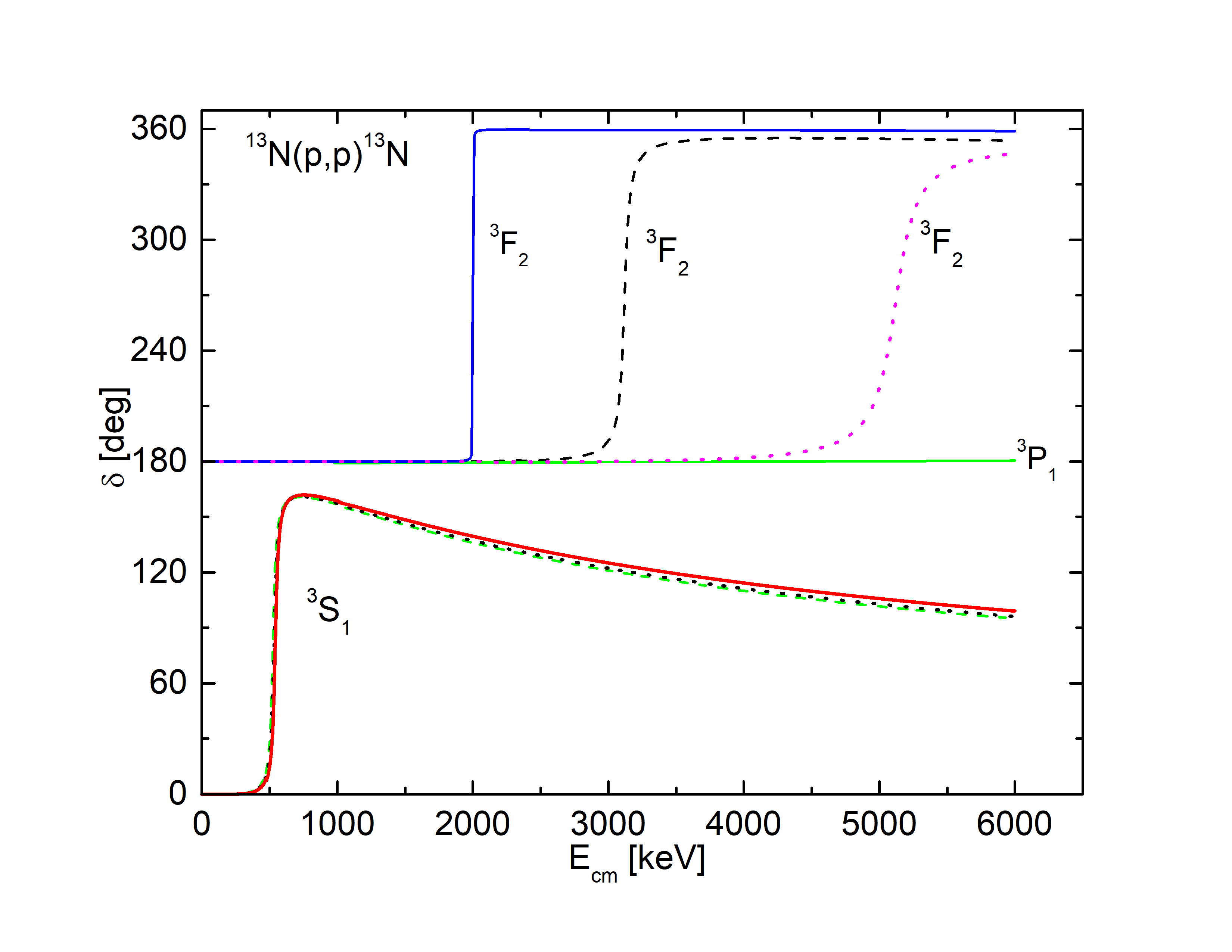
Figure 1: The dependence of the elastic $p^{13}N$ scattering phases on the energy. Calculations are performed using the potentials with parameters from Table 1. The ${}^{3}S_{1}$ phase shift is calculated using the set 1$a$ (green dashed curve), 1$b$ (black dotted curve) and 1$c$ (red solid curve) from Table 1, respectively. The three sets of parameters for the potential give almost the coincide results for the ${}^{3}S_{1}$ phase shift. In the given energy region the ${}^{3}P_{1}$ phase shift has very weak energy dependence.

In calculations we use for the proton mass $m_{p}=1.007276469$ amu 8 and ¹³N mass 13.0057367 amu 9 , where 1 amu $=$ 931.4941024 MeV 8 and the constant $\hbar^{2}/m_{0}=41.4686$ MeV$\cdot$fm². The Coulomb potential at $R_{C}=0$ is written in MeV as $V_{C}(r)=1.439975Z_{1}Z_{2}/r$, where $r$ is the interparticle distance in fm, $Z_{1}$ and $Z_{2}$ are charges of the particles in units of the elementary charge. The Sommerfeld parameter $\eta=\mu Z_{1}Z_{2}e^{2}/(k\hbar^{2})=3.44476\text{\textperiodcentered}10^{-2}\mu Z_{1}Z_{2}/k$, where $k=\left(2\mu E/\hbar^{2}\right)^{1/2}$ is the wave number specified in fm^-1 and defined by the energy $E$ of interacting particles, and the reduced mass $\mu$ of these particles in amu.

Following Ref. Nichitiu1980 for calculations of the width employing the resonance scattering phase we use the expression $\Gamma_{res}=2(d\delta/dE)^{-1},$ where $\delta$ is the phase shift. For description of ${}^{3}S_{1}$, ${}^{3}P_{1}$, and ${}^{3}F_{2}$ scattering states we use the corresponding experimental energies and widths. For the ${}^{3}S_{1}$ resonance there are reported three different experimental measurements for the resonance energy and width. Therefore, we constructed the potential for the ${}^{3}S_{1}$ resonance scattering phase with three sets of parameters. In Table 1 are given the results of calculations of parameters for the corresponding potential. The potential with sets of parameters 1$a,$ 1$b,$ and 1$c$ reproduce the resonance energies 528, 536 and 545 keV, respectively. The latter allows to find the optimal astrophysical $S$-factor. In Fig. 1 the dependence of the elastic $p^{13}N$ scattering phase shifts on the energy $E_{cm}$. The result of calculation of the ${}^{3}S_{1}$ phase shift with the set 1$c$ parameters for the $S$ scattering potential without FS leads to 90${}^{0}\pm$1⁰ at the energy $E_{res}=0.545$ MeV 12 are presented by the red solid curve. The calculations of the ${}^{3}S_{1}$ phase using the sets of parameters 1$a$ and 1$b$, which correspond to the resonances at $E_{res}=0.528$ MeV 14 and $E_{res}=0.536$ MeV 15 give the coincide results in Fig. 1. Thus, the scattering potentials with the set of parameters 1$a$, 1$b$ and 1$c$ are phase shift equivalent potentials.

The potential of the nonresonance scattering is also constructed quite unambiguously based on the scattering phase shifts for a given number of bound states allowed and forbidden in the partial wave. The accuracy of determining the parameters of such a potential is primarily associated with the accuracy of extracting the scattering phase shifts from the experimental data. Since the classification of states according to Young diagrams makes it possible to unambiguously fix the bound states number, which completely determines its depth, the potential width at a given depth is determined by the shape of the scattering phase shift. When constructing a nonresonance scattering potential from the data on the spectra of the nucleus, it is difficult to evaluate the accuracy of finding its parameters even for a given number of bound states. Such a potential, as is usually assumed for the energy range up to $1-3$ MeV, should lead to the scattering phase shift close to zero or gives a smoothly decreasing phase shift shape, since there are no resonance levels in the spectra of the nucleus.

For the ${}^{3}P_{1}$ scattering potential, one can use the parameter set 2 from Table 1. Such a potential has the FS and leads to scattering phase shift of 180${}^{0}\pm$1⁰, which has a very weak dependence of energy and is presented by the green solid curve in the energy range from zero to 7 MeV. Since it has the FS, according to the generalized Levinson theorem, its phase shift begins at 180⁰ 7 .

Table 1: List of transitions from the initial $\left\{{}^{\left(2S+1\right)}L_{J}\right\}_{i}$ state to ${}^{3}P_{0}$ GS of ¹⁴O nucleus. The value of $P^{2}$ determines the coefficient in expressions (3) and (9). The width $\Gamma_{res}$ and $S(0)$-factor are obtained using the potential parameters $V_{0}$ and $\alpha.$ The value $\widetilde{S}(0)$ of the $S$-factor and the set of parameters $1d$, $1e$, and $1f$ for the potential are used for calculations of the resonance width $\widetilde{\Gamma}_{res}.$

Set	{${}^{(2S+1)}L_{f}$}i	Transition	$P^{2}$	$V_{0},$ MeV		$\alpha,$ fm-2	$E_{res},$ MeV	$\Gamma_{res},$ keV	$S(0)$, keV$\cdot$b	$\widetilde{\Gamma}_{res}$, keV	$\widetilde{S}(0)$, keV$\cdot$b
				a	14.955	0.085	0.528(1)	37(1)	8.4(2)
				b	15.882	0.092	0.536(1)	38(1)	7.9(2)
1	${}^{3}S_{1}$ resonance at	$E1$	1	c	18.244	0.11	0.545(1)	37(1)	7.0(2)
	$0.528,0.536,0.545$ MeV			d	35.053	0.25	0.528(1)			22(1)	4.8(1)
				e	29.316	0.02	0.536(1)			25(1)	5.1(1)
				f	31.582	0.22	0.545(1)			26(1)	4.9(1)
2	${}^{3}P_{1}$ no resonance	$M1$	2	555.0		1.0			0.014(1)
3	${}^{3}F_{2}$ resonance at 1.981(10)	$E2$	3	698.134		0.36	2.000	13	$<$ 0.01
4	${}^{3}F_{2}$ resonance at 3.117(19)	$E2$	3	343.613		0.18	3.120	58	$<$ 0.01
5	${}^{3}F_{2}$ resonance at 5.123(11)	$E2$	3	430.2		0.23	5.127	232	$<$ 0.01

We also considered the $J^{\pi}=2^{+}$, $E_{res}=1.981(10)$ MeV, $\Gamma_{res}=5$ keV, $J^{\pi}=2^{+},$ $E_{res}=3.140(10)$ MeV, $\Gamma_{res}=68(6)$ keV, and $J^{\pi}=2^{+},$ $E_{res}=5.123(11)$ MeV, $\Gamma_{res}=229(51)$ keV resonances, which lead to a noticeable change in the $S$-factor in resonance regions, using the potentials with the parameters set 3, 4 and 5, respectively, from Table 1. However, it was not possible to construct such potentials in $P-$waves, therefore, $F$ scattering waves were used here. The first of them leads to a resonance at 2.00 MeV with a width $\Gamma_{res}=13$ keV shown by the blue solid curve in Fig. 1, the second gives the resonance at $E_{res}=3.12$ MeV and a width $\Gamma_{res}=58$ keV and is presented by the black dashed curve, while the phase shift of the third resonance at $E_{res}=5.127$ MeV is shown by the dotted curve. We were not able to obtain the resonance at $E_{res}=1.981$ MeV with the width $\Gamma_{res}<5$ keV, as given in 14 , but the obtained value is completely consistent with the recent data 15 .

To build the potential for description of the GS of ¹⁴O,  we use the experimental binding energy and the asymptotic normalization coefficient ($ANC$) of this state. The corresponding potentials are tested based on the calculation of the root mean square charge radius of ¹⁴O.

In Ref. 16 the value of $ANC=5.42(48)$ fm^-1/2 and the proton spectroscopic factor $S_{p}=1.88(34)$ are given. A similar value of $ANC=5.42(74)$ fm^-1/2 is also reported in Ref. 17 , while Ref. 18 reports $ANC=5.39(38)$ fm^-1/2. Using the results of 16 for the $ANC$ and the expression for the asymptotic normalization constant

$$ANC=\sqrt{S_{p}}C$$ (13)

one gets $C=$4.04(72) fm^-1/2. For determination of $C$, the following definition is also used (see, for example, 19 )

$$\chi_{L}(r)=CW_{-\eta,L+1/2}(2k_{0}r),$$ (14)

where $W_{-\eta,L+1/2}(2k_{0}r)$ is a Whittaker function. We use a different definition of $ANC$ 20

$$\chi_{L}(r)=\sqrt{2k_{0}}C_{w}W_{-\eta,L+1/2}(2k_{0}r)$$ (15)

which differs from the previous definition by the factor $\sqrt{2k_{0}}$ which in this case is 0.956. Then for the dimensionless $C_{w}$ we get $C_{w}=4.23(75)$. At the same time in Ref. 18 $S_{p}=0.90(23)$ was given for the spectroscopic factor, which yields $ANC=5.39(38)$ fm^-1/2 and allows to obtain $C_{w}=6.15(1.22)$. $ANC=30.4(7.1)$ fm^-1 and $S_{p}=1.94(45),$ were obtained in Ref. 25 , which lead to the dimensionless asymptotic normalization constant within the range 3.26 – 5.30 with an average of 4.28(1.02).

The potential of a bound ground ${}^{3}P_{0}$ state with the FS should correctly reproduce the GS energy –4.628 MeV of ¹⁴O nucleus with $J^{\pi}=0^{+}$ in the $p^{13}$N channel 12 and it is reasonable to describe the mean square radius of ¹⁴O as well. Since data on the radius of ¹⁴O are not available, we consider it to coincide with the radius of ¹⁴N, the experimental value of which is 2.5582(70) fm 9 . As a result, we obtained the following parameters for the GS potential, which lead to $C_{w}=4.1(1)$:

$$V_{0}(1,1,0^{+})=226.230\text{ MeV, }\alpha(1,1,0^{+})=0.23\text{ fm}^{-2}.$$ (16)

The potential (12) with the parameters (16) gives for the ¹⁴O nucleus the binding energy of 4.628 MeV and the root mean square charge radius $R_{ch}=$ 2.55 fm. We used 0.8768(69) fm for the proton radius 8 and 2.4614(34) fm for the ¹³N radius. The latter radius was taken to be the radius of ¹³C 9 , because the ¹³N radius is not available.

The GS potential which leads to $C_{w}=6.1(1)$ has parameters

$$V_{0}(1,1,0^{+})=156.728\text{ MeV, }\alpha(1,1,0^{+})=0.15\text{ fm}^{-2}.$$ (17)

The GS potential with parameters (17) gives a binding energy of 4.628 MeV and the root mean square charge radius $R_{ch}=$ 2.63 fm. One can see that the potential (14) gives a larger radius than the potential (13), so by simple estimates it is clear the GS with (14) should have larger cross sections.

We calculated the radial WFs of GSs and shape of the integrand in matrix element ME (5) of the $E1$ transition using the scattering potential with the set of parameters 1$a$ and 1$c$ from Table I. The results of calculations are presented in Fig. 2. The radial WFs for the GS of ¹⁴O in the $p$¹³N channel obtained with potentials (17) and (17) are shown in Fig. 2$a$. The GS WFs have the same behavior, different magnitudes and the shifted nodes. The different magnitudes lead to the different shape of the integrand in the ME (5) of the $E1$ transition, which also depends on the choice of the parameters for the potential for the description of the scattering state. The node in the nuclear interior leading to the node in the integrand shown in Fig. 2$b$ and 2$c$, respectively. We should be noted that integrands in the ME (5) of the $E1$ transition almost coincide with the integrand shown in Fig. 8 in Ref. 18 .

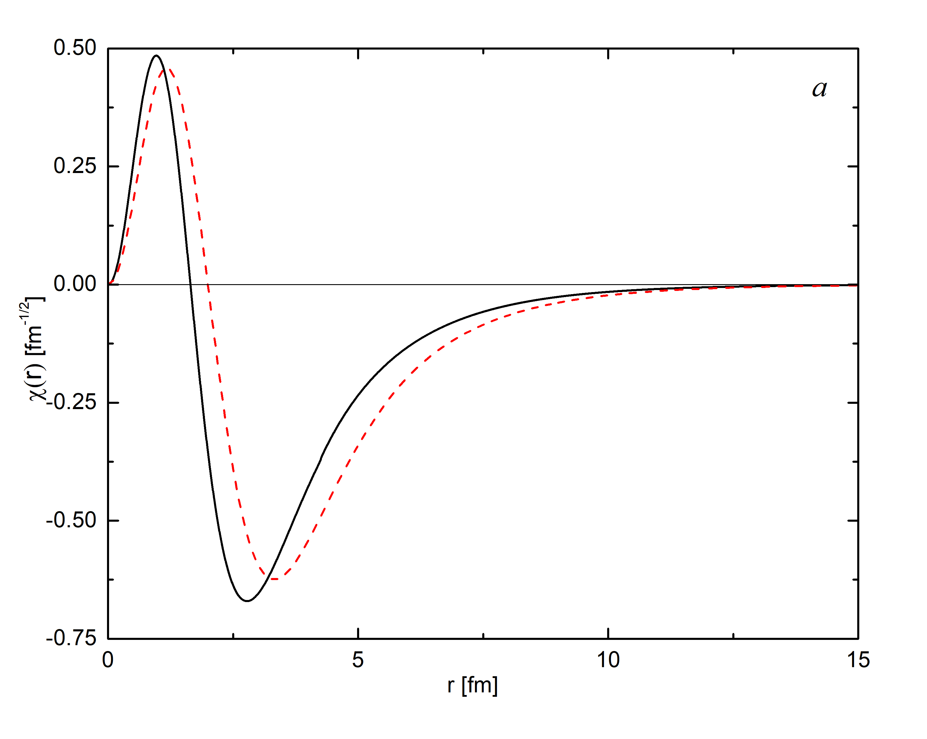
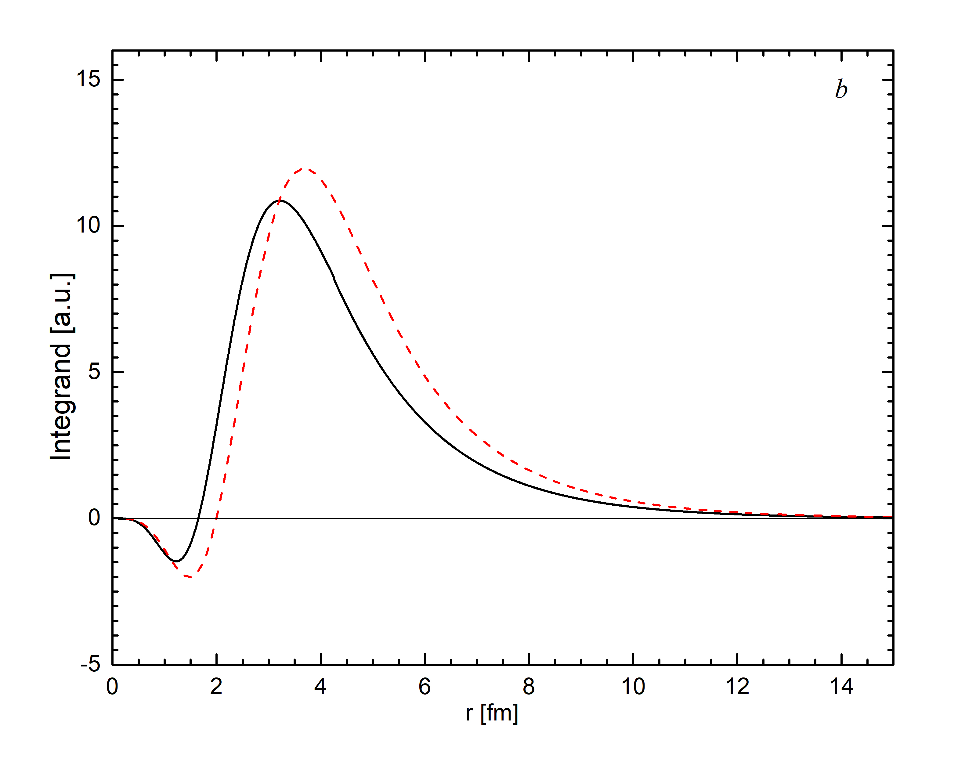
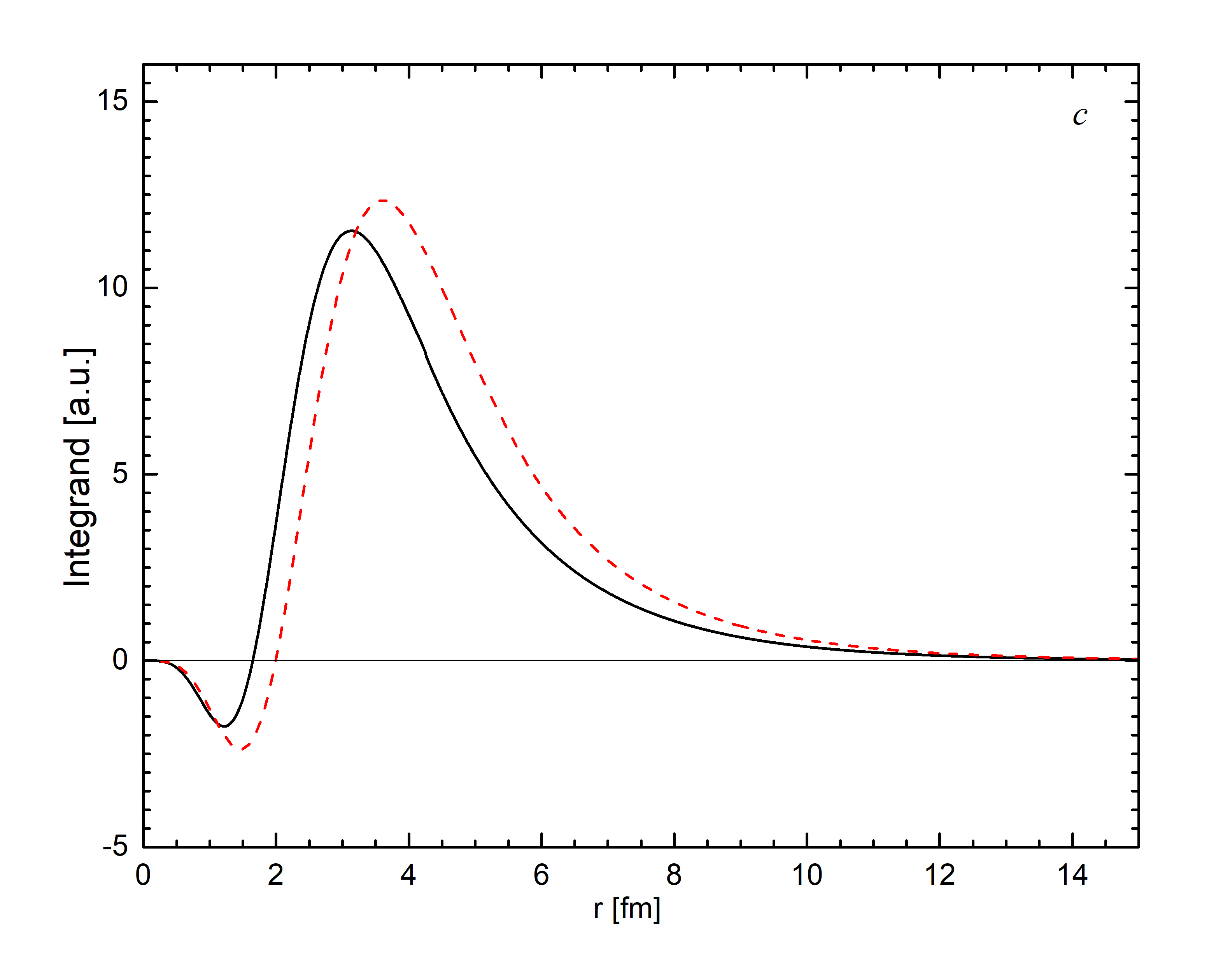
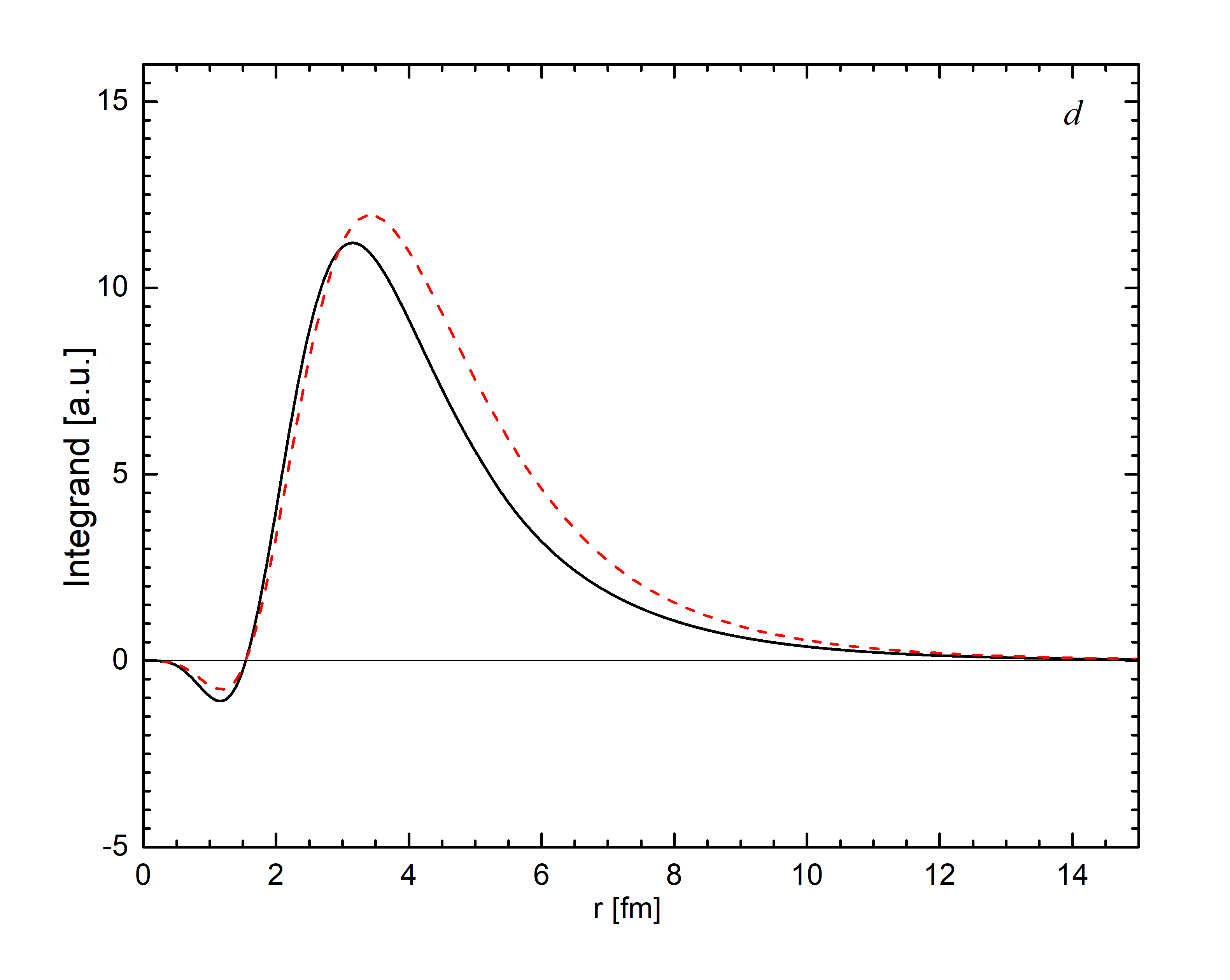
Figure 2: (Color online) The radial part of the GS wave functions ¹⁴O in the $p^{13}$N channel and integrands in the matrix element (5) for the $E1$ transition in arbitrary units (a.u.). (a) The GS wave function obtained with potential (16) (solid curve) and potential (17) (dashed curve). (b) The integrand of the $E1$ transition ME (5) for the scattering potential with the set of parameters 1$a$ from Table I and for the GS potential (16) (solid curve) and (17) (dashed curve), respectively. (c) The integrand of the $E1$ transition ME (5) for the scattering potential with the set of parameters 1$c$ from Table I and for the GS potential (16) (solid curve) and (17) (dashed curve), respectively. (c) The integrand of the $E1$ transition ME (5) for the scattering potential with the set of parameters 1$c$ from Table I and for the GS potential (16) (solid curve) and (17) (dashed curve), respectively. (d) The integrand of the $E1$ transition ME (5) for the GS potential without FS (18) at $C_{W}=4.1$ (solid curve) and the GS potential without FS (19) at $C_{W}=6.0$ (dashed curve) and for the scattering potential (20), respectively.

One should be noted that the shell model is undoubtedly the most perfectly formulated from both a physical and mathematical point of view. In fact, on the one hand, in the framework of shell model, the Pauli principle is precisely taken into account. On the other hand, this model allows, based on algebraic methods, to take into account the effects of clustering in atomic nuclei. Thus, the shell model could be recognized as a criterion for testing the “quality’ of other models using phenomenological nucleon-cluster potentials. Let us for comparison consider the GS potentials without FS and scattering potentials with the FS in the ${{}^{3}}S{{}_{1}}$ wave based on a single-particle model. The GS potential without the FS has parameters:

$$V_{0}(1,1,0^{+})=61.23803\text{ MeV, }\alpha(1,1,0^{+})=0.13\text{ fm}^{-2}.$$ (18)

This potential leads to the binding energy of 4.62800 MeV, root-mean-square charge radius $R_{ch}=2.54$ fm and $C_{w}=4.1(1)$. This completely coincides with the option for potential (16). One can also obtain another option for the GS potential, which agrees with the shell model of the system, which has parameters:

$$V_{0}(1,1,0^{+})=45.46913\text{ MeV, }\alpha(1,1,0^{+})=0.085\text{ fm}^{-2}.$$ (19)

This potential leads to the binding energy of 4.62800 MeV, root-mean-square charge radius $R_{ch}=2.61$ fm and $C_{w}=6.0(1)$. This coincides with the option for potential (17). The scattering potential for the resonance ${{}^{3}}S{{}_{1}}$ wave now has the FS and parameters:

$$V_{0}(1,1,0^{+})=125.529\text{ MeV, }\alpha(1,1,0^{+})=0.24\text{ fm}^{-2}.$$ (20)

This potential leads to the resonance energy of 545 keV and its width of 37(1) keV, this is completely coinciding with results for the set 1$c$ from Table 1. The shape of the integrands in the ME (5) of the $E1$ transition for the GS potentials (18) and (19), and scattering potential (20) is shown in Fig. 2$d$.

We use the potentials with parameters from sets $1a$, $1b$ and $1c$ in Table 1 for the description of the resonance states and parameters (16) and (17) for the description of the residual ¹⁴O nucleus for calculations of the ¹³N($p,\gamma)^{14}$O reaction rate and the astrophysical $S$-factor.

The astrophysical $S$-factor was calculated previously using the ${}^{3}S_{1}$ resonance scattering. Using the values of $\widetilde{S}(0)$ from Table 1, we consider the inverse problem to construct potentials for description the ${}^{3}S_{1}$ resonance based on the resonance energies and the corresponding astrophysical $S$-factor. The parameters of these potentials are given in Table 1 as sets $1d$, $1e$ and $1f$.

V Reaction rate and astrophysical $S$-factor of the proton radiative capture on ¹³N

Let us calculate the reaction rate for the ¹³N($p,\gamma$)¹⁴O radiative capture and the astrophysical $S$-factor using the total cross section (2) and corresponding matrix elements of multipole transition operators. The astrophysical factor $S(E)$ is defined as

$$S(E)=E\sigma_{c}(NJ,J_{f})e^{-2\pi\eta},$$ (21)

where the factor $\exp(-2\pi\eta)$ approximates the Coulomb barrier between two point-like particles with charges $Z_{1}$ and $Z_{2}$ and orbital momentum $L=0$, while for the reaction rate is commonly expressed in cm³mol^-1s^-1 and is determined according to Ref. 28 ; Fowler as

$$N_{A}\left\langle\sigma_{c}v\right\rangle = N_{A}\frac{2(2/\pi)^{1/2}}{\mu^{1/2}(k_{B}T)^{3/2}}\int_{0}^{\infty}\sigma_{c}(E)E\exp\left(-E/k_{b}T\right)dE$$ (22)

$$= 3.7313\times 10^{4}\mu^{-1/2}T_{9}^{-3/2}\int_{0}^{\infty}\sigma_{c}(E)E\exp\left(-11.605E/T_{9}\right)dE,$$

where $N_{A}$ is Avogadro’s number, $k_{B}$ is the Boltzmann’s constant, $E$ is the energy in the center-of-mass frame given in MeV, the cross section $\sigma_{c}(E)$ is measured in $\mu$b, $\mu$ is the reduced mass in a.m.u, and $T_{9}$ is the temperature in units of $10^{9}$ K. The behavior of $S$-factor, when resonances are present, in general, is expected to be rather smooth at low energies and can be expanded in Taylor series around $E=0$ Baye2000 ; Ryan as

$$S(E)=S_{0}+ES_{1}+E^{2}S_{2}.$$ (23)

Essentially, the experimental data on the astrophysical $S$-factor of the proton radiative capture on ¹³N are absent, but in the database 21 there are rates of this reaction from Refs. 16 ; 22 . However, it is clear that the shape of $S$-factor should mainly be determined by resonance in the ${}^{3}S_{1}$ scattering wave at 0.528 MeV with a width $\Gamma_{res}=37.3(9)$ keV and $J^{\pi}=1^{-}$ 14 . The contributions of cross sections of ${}^{3}F_{2}$ resonances from Table 1, which are determined by $E2$ transitions, are possible as well.

For calculations of the astrophysical $S$-factor we use the potentials with parameters from sets $1a$, $1b$ and $1c$ in Table 1 for the description of the resonance state and parameters (16) and (17) for the description of the residual ¹⁴O nucleus. We also calculate the width of ${}^{3}S_{1}$ resonance using the sets of the parameters $1d$, $1e$ and $1f$ for the potentials from Table 1, which were obtained based on the values of the astrophysical $S$-factor.

The results of calculation of the $S$-factor of the radiative proton capture on ¹³N to the GS of ¹⁴O nucleus include the sum of $E1$, $E2$ and $M1$ transitions are shown in Fig. 3. For the contribution of the ${}^{3}S_{1}$ scattering wave the set of parameters from Table 1 for the potential and potential (16) for the GS are considered. We calculated the contributions of the $M1$ transition ${}^{3}P_{1}\rightarrow$ ${}^{3}P_{0},$ as well as the resonance $E2$ transitions into the $S$-factor using the set of the potentials 2, 3, 4, and 5 from Table 1, respectively, and for the description of the GS the potential (16) was used. The results of these calculations are shown in Fig. 3$a$. Analysis of results presented in Fig. 3$a$ shows that contributions of the $M1$ and $E2$ transitions in the $S$-factor are negligible at energies $E<1$ Mev, but are significant at high energies. At the resonance energy, the $S$-factor reaches 2.4 MeV$\cdot$b, which is in good agreement with the results of other works (see, for example, Refs. 16 ; 18 ; 22 ; 23 ), where the values for the $S$-factor from about 2.0 to 2.5 keV·b were reported. The $S$-factor shown in Fig. 3$b$ is given for three sets of parameters $1a$, $1b$ and $1c,$ highlighting the differences. Results of our calculations for the $S$-factor for the potentials $1a$ from Tables 1 and (16) in the energy range of $30-50$ keV lie in the range of $8.2-8.3$ keV$\cdot$b, while in the energy range of 30–70 keV, the average value is 8.4(2) keV$\cdot$b. The error given here is determined by averaging $S$-factor over the above energy range. Known results for the $S-$factor at zero energy lead to a value in the range from 2.0 keV$\cdot$b to 6.0 keV$\cdot$b 16 ; 18 ; 22 ; 23 . We use the GS potential (17) and calculate the $S$-factor in the energy range $30-70$ keV using the set of parameters $1a$ from Table 1 for the potential and obtain almost constant value $S=11.9(2)$ keV·b. At the resonance energy the $S$-factor reaches 2.9 MeV$\cdot$b, which is noticeably more than the results of 16 ; 18 ; 22 ; 23 . Therefore, we should mention that the GS potential with the parameters (16) for description of the GS of ¹⁴O nucleus in the $p^{13}$N channel at low energy region leads to more preferable results for the astrophysical $S$-factor, which are quite consistent with results from previous calculations. Our calculations for the $S$-factor with the parameters (17) for the potential of the GS gives a too high value for the $S$-factor at low energies. However, since there are no experimental measurements of the $S$-factor for this reaction, no final conclusions can be drawn.

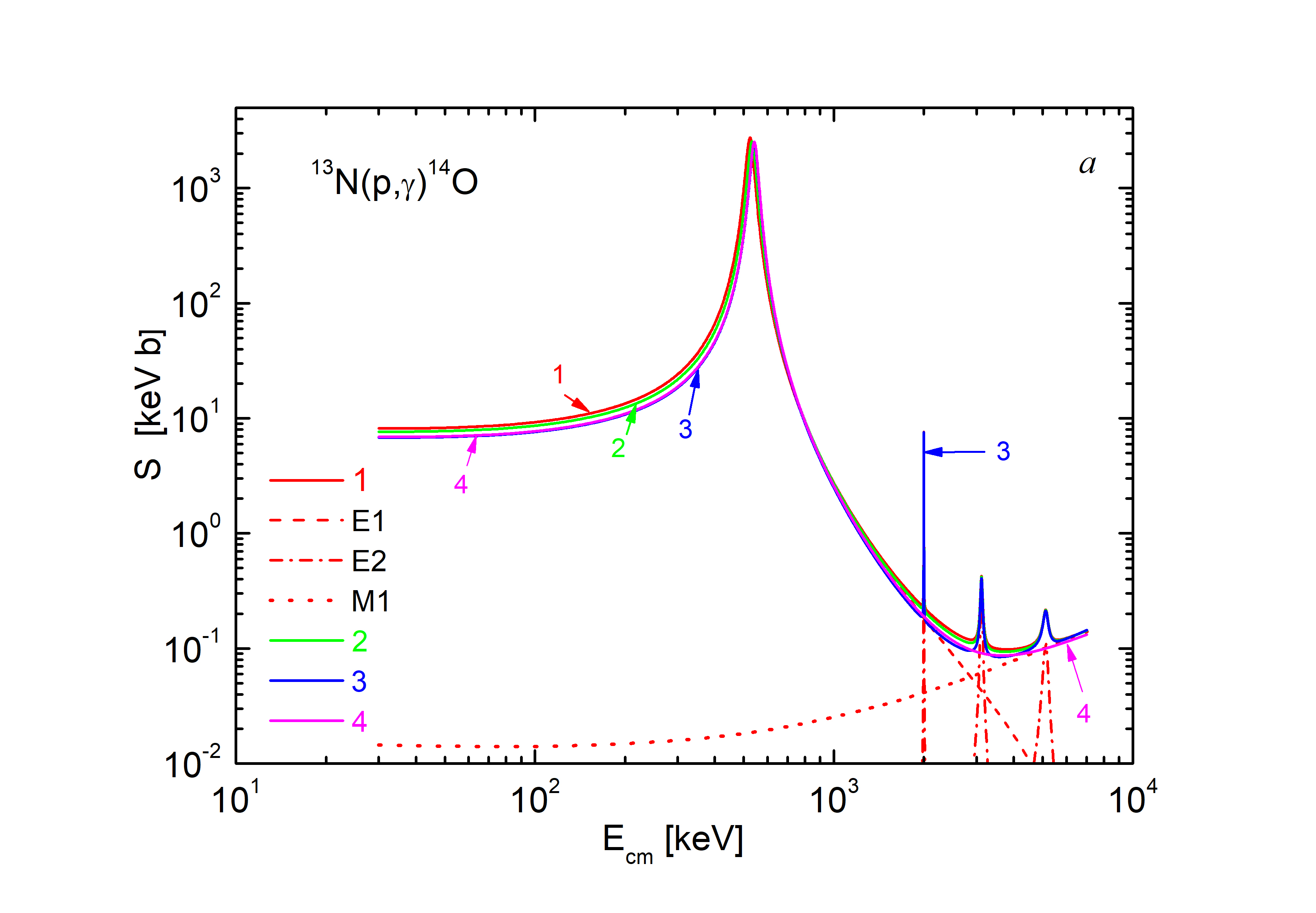
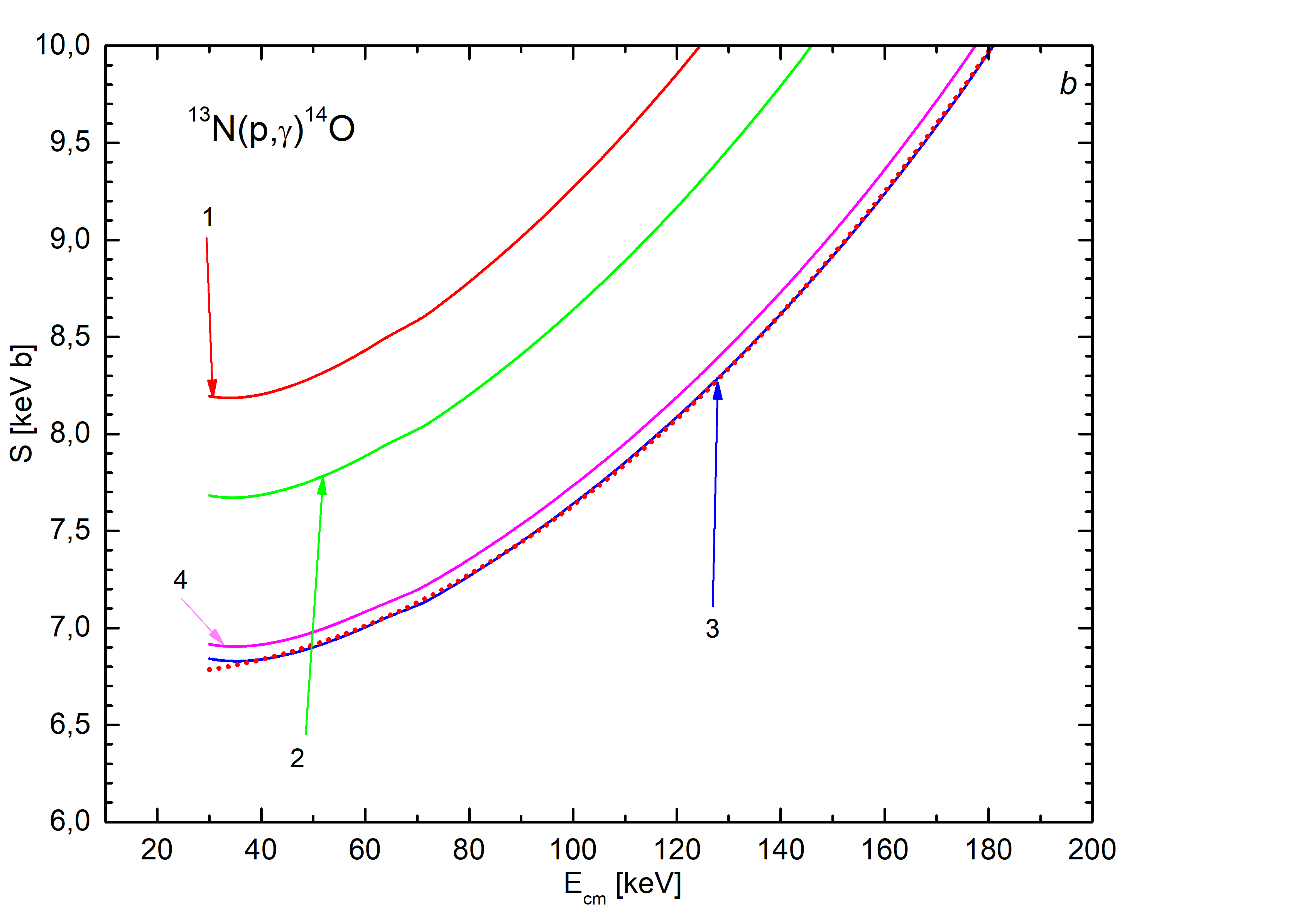
Figure 3: (Color online) Astrophysical $S-$factor of the radiative proton capture on ¹³N. ($a$) The energy range 30 keV – 7 MeV. The solid curves 1–4 present results of calculations which include the sum of $E1$, $E2$ and $M1$ transitions. Results presented by curves 1–3 are obtained using potential with the set of parameters 1$a$, 1$b$ and 1$c$ from Table 1, respectively, and the GS potential (16). The curve 4 corresponds the ”node inversion” in $E1$ transition simulated by the GS potential without FS (18) and scattering potential (20) The dashed, dash-dotted and dotted curves illustrate the contributions of the $E1$, $E2$ and $M1$ transitions, respectively, into $S-$factor obtained for the potentials with the set of parameters 1$a$ from Table 1 and GS (16). ($b$) The energy range 30 – 200 keV. The solid curves 1, 2, 3 and 4 present the same results as in Fig. 3$a$. The red dotted curve, which coincides with the curve 3, presents the quadratic approximation (23) of the $S$-factor at low energies.

Table 2: Astrophysical $S$-factors at zero energy.

Refs.		24	16 ; 17 ; 18 ; 23 ; 25 a	26 b	[27]a
$S$, keV$\cdot b$		$3.8_{-08}^{+1}$	$5-6$	$2.6$	$2-2.3$
aValues are taken from Figures in Refs: [16] – Fig. 7; [17] – Fig. 8;
[18] – Fig. 9; [23] – Fig. 5; [25] – Fig. 3; [27] – Fig. 2b.
bValue is taken from the approximation at low energies.

Table 2 displays the compilation of the results for the astrophysical $S$-factors at zero energy obtained in different works. As can be seen from Table 2, the deviation of data for the $S$-factor is in the range from 2 to 6 keV·b, although the most recent value is apparently given in Ref. 24 . We use the sets of parameters $1a$, $1b$, and $1c$ for the potential of ${}^{3}S_{1}$ scattering from Table 1 and potential (16) for the GS, which reproduce accurately the position and width of resonances and calculated corresponding $S$-factors. The results are presented in Table 1. Depending on the resonance energy $S$-factors are: 8.4(2) keV$\cdot$b ($E_{res}=528(1)$ keV), 7.9(2) keV$\cdot$b ($E_{res}=536(1)$ keV), and 7.0 keV$\cdot$b ($E_{res}=545(1)$ keV). The potential with the set $1a$ from Table 1 accurately reproduces the width average value of 37 keV 14 and leads to $S(0)=8.4(2)$ keV$\cdot$b. The potential with the set $1b$ reproduces the resonance energy of 536(12) keV and the width $\Gamma_{res}=38(2)$ keV from Ref. 15 . The corresponding average value for the $S$-factor at 30–70 keV is $S(0)=7.9(2)$ keV$\cdot$b, which is slightly less than for the $S$ scattering potential $1a.$ We consider a potential with parameters $1c$, which leads to the resonance at 545 keV and a width $\Gamma_{res}=37(1)$ keV 12 . This potential gives $S(0)=7.0(2)$ keV$\cdot$b.

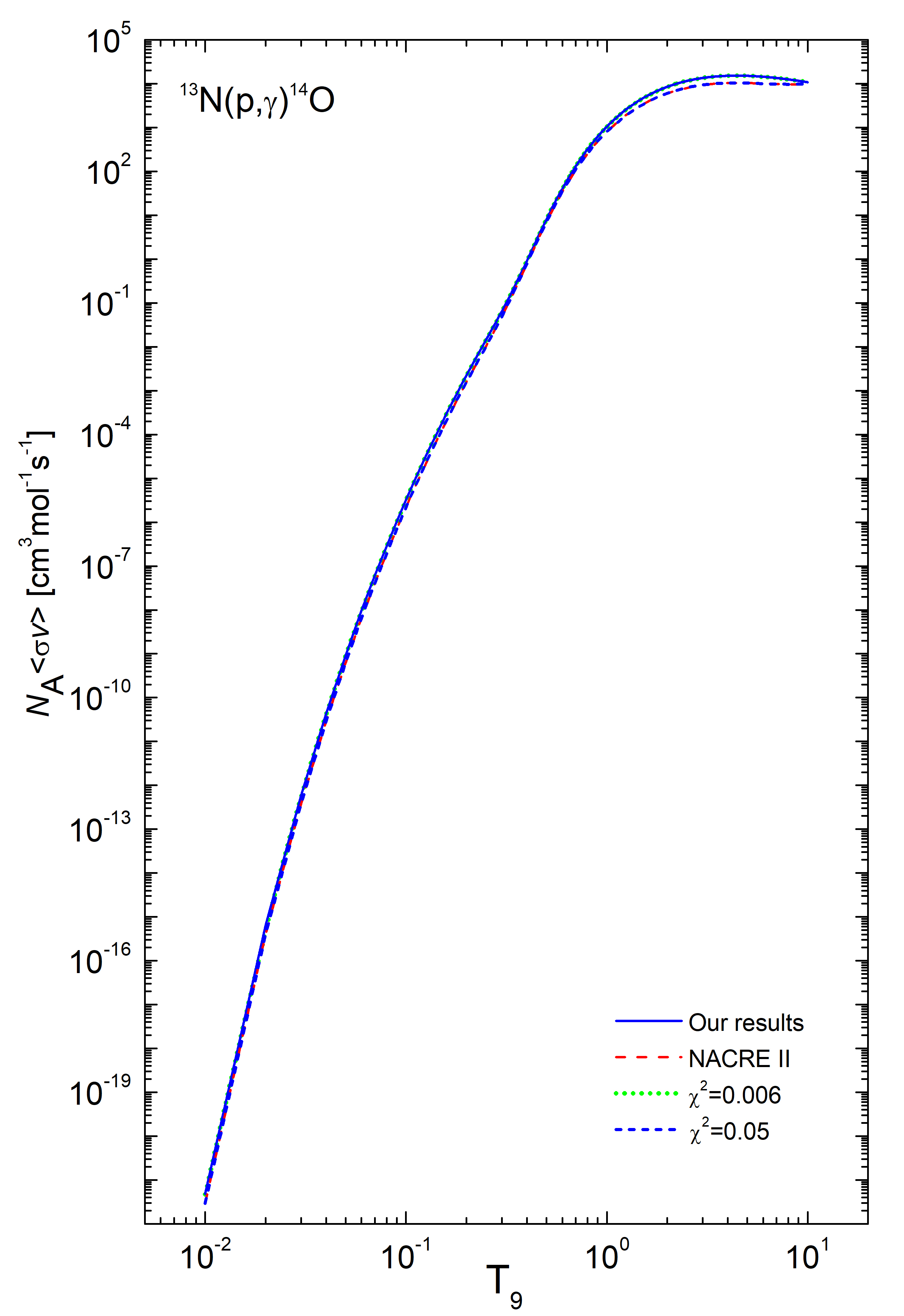
Figure 4: (Color online) The dependence of the reaction rate of $p^{13}N$ radiative capture on astrophysical temperature. The solid curve presents our calculations for the sum of $E$1, $M1$ and $E2$ transitions performed for the potentials with the set of parameters 1$c$ from Table (1) and GS (16). Results of parametrization by Eq. (21)(24) with parameters from Table 4 for the present calculations and the NACRE II data 24 are shown by the dotted and dashed curves, respectively. The short dashed curve shows the calculations using approximation (23).

Table 3: The results of the dependence of the $p^{13}N$ reaction rate on temperature.

Temperature, $T_{9}$	Reaction rate, cm3mol-1s-1	Temperature, $T_{9}$	Reaction rate, cm3mol-1s-1
0.01	4.81E-22	0.35	2.53E-01
0.02	6.46E-16	0.4	9.10E-01
0.03	5.94E-13	0.45	2.91E+00
0.04	4.37E-11	0.5	8.04E+00
0.05	9.28E-10	0.6	4.02E+01
0.06	9.54E-09	0.7	1.30E+02
0.07	6.14E-08	0.8	3.13E+02
0.08	2.86E-07	0.9	6.13E+02
0.09	1.05E-06	1	1.04E+03
0.1	3.22E-06	1.5	4.53E+02
0.11	8.61E-06	2	8.46E+03
0.12	2.06E-05	2.5	1.15E+04
0.13	4.49E-5	3	1.35E+04
0.14	9.09E-05	3.5	1.46E+04
0.15	1.73E-04	4	1.51E+04
0.16	3.12E-04	4.5	1.52E+04
0.17	5.37E-04	5	1.51E+04
0.18	8.90E-04	6	1.44E+04
0.19	1.42E-03	7	1.35E+04
0.2	2.21E-03	8	1.25E+04
0.25	1.40E-02	9	1.16E+04
0.3	6.46E-02	10	1.08E+04

Table 4: Parameters of the analytical parametrization of the ¹³N($p,\gamma$)¹⁴O reaction rate for the present calculations based on Eq. (24) and NACRE II data 24 based on Eq. (24) as well.

Parameters	$a_{1}$	$a_{2}$	$a_{3}$	$a_{4}$	$a_{5}$	$a_{6}$	$a_{7}$
Present work, Eq. (24)	$4.68425$	$5.5271$	$72207.8$	$-2.86832$	$-17716.6$	$-1304.726$	$-1155.274$
NACRE II	$77.14845$	$4.87776$	$-2791.957$	$7554.465$	$-4686.978$	$3691.79$	$-4033.686$
Parameters	$a_{8}$	$a_{9}$	$a_{10}$	$a_{11}$	$a_{12}$	$a_{13}$	$a_{14}$
Present work, Eq. (24)	$-1020.536$	$215.4007$	$4.66187\times 10^{6}$	$10.92388$	$8.5529\times 10^{7}$	$15.50687$	$16674.76$
NACRE II	$1901.048$	$-309.4704$	$-3320.309$	$7.12181$	$3.13709\times 10^{8}$	$15.87507$	$-13.31191$
Parameters			$a_{15}$	$a_{16}$	$a_{17}$
Present work, Eq. (24)			$7.86955$	$-77.74082$	$1.38331$
NACRE II			$5.65906$	$-48.07274$	$1.23332$

Nevertheless, let us try to find out whether it is possible within our approach to obtain the $S$-factor at zero energy that is close to the results of 24 , namely, $3.8_{-08}^{+1}$ keV·b. We constructed $S-$wave scattering potentials, which with the potential (16) for the GS, allow us to obtain maximum value of the $S-$factor about $4.8-5.0$ keV$\cdot$b given in Ref. 24 . Such potentials have the set of parameters $1d,$ $1e,$ and $1f$ listed in Table 1. These potentials lead to the resonance energies $528(1)$ keV, $536(1)$ keV, and 545(1) keV, respectively, but the corresponding widths are significantly smaller than reported in Refs. 14 ; 15 ; 12 . In particular, the set $1d$ leads to $E_{res}=528(1)$ keV, but the width is $\widetilde{\Gamma}_{res}=22(1)$ keV. At 30 keV $\widetilde{S}(0)=$4.8 keV$\cdot$b and its average value in the range of $30-70$ keV is $\widetilde{S}(0)=4.8(1)$ keV$\cdot$b. If for the potential with a resonance energy of 536 keV, we use the parameters $1e$ from Table 1, which lead to $\widetilde{\Gamma}_{res}=25(1)$ keV, then the $S$-factor decreases to $\widetilde{S}(0)=5.1(1)$ keV$\cdot$b. The $S$-factor decreases to $\widetilde{S}(0)=4.9(1)$ keV$\cdot$b, when we use the set $1f$ for the potential and the width becomes $\widetilde{\Gamma}_{res}=26(1)$ keV. Thus, in principle, all previously obtained results for the $S$-factor at zero energy can be reproduced, but the width of the resonances does not correspond to the data 14 ; 15 ; 12 . Therefore, for the considered resonance energies, if we correctly describe their widths, it is impossible to obtain the $S$-factor below 7.0 (2) keV$\cdot$b. Only a decrease in the resonance width to 25–26 keV with its energy of 536–545 keV leads to the $S$-factor of the order of 4.9–5.1 keV$\cdot$b.

We also calculated the $S$-factor using the GS potential (18) without FS and the scattering potential (20). The result for the average value of the $S$-factor in the range of 30-70 keV is 7.0(1) keV$\cdot$b that completely coincides with the $S$-factor, calculated with the parameters set 1$c$ from Table 1 and GS potential (16). We use Eq. (23) for the approximation of the $S-$factor at low energies. The corresponding parameters are: $S_{0}=6.7645$, $S_{1}=-2.7612\times 10^{-3}$, $S_{2}=1.1428\times 10^{-4}$ at $\chi^{2}=1.0\times 10^{-3}$. The results are shown in Fig. 3$b$ by the dotted curve that coincides with the curve 3, which presents the results of calculations for the potentials with the set of parameters 1$c$ from Table 1 and GS (16).

Using Eq. (22), we calculated the rate of the ¹³N($p,\gamma$)¹⁴O radiative capture by considering the sum of $E$1, $M1$ and $E2$ transitions. The dependence of the ¹³N($p,\gamma$)¹⁴O reaction rate on astrophysical temperature is shown in Fig. 4. The corresponding rates are tabulated in Table 3 for $0.01<T_{9}<10$. The calculations are performed using the set of parameters $1c$ and (16) for the potentials. Let us mention that the earlier calculations 16 ; 18 ; 23 practically coincide with our results with small deviations, while results from Ref. 22 at temperatures $T_{9}>1$ are up to 2 times lower than present results. The results of calculations with the set of parameters $1c$ and (17) for the potentials give a noticeable excess of the reaction rate over the rates obtained with the GS potential (16) at temperatures above 1 $T_{9}.$

Following Ref. 29 the reaction rate obtained in our calculations is parameterized as

$$N_{A}\left\langle\sigma v\right\rangle = \frac{a_{1}}{T}\exp\left(-\frac{a_{2}}{T}\right)\left(1+a_{3}T^{1/3}+a_{4}T^{2/3}+a_{5}T^{4/3}+a_{7}T^{5/3}+a_{8}T^{6/3}+a_{9}T^{7/3}\right)+$$ (24)

$$\frac{a_{10}}{T^{1/2}}\exp\left(-\frac{a_{11}}{T^{1/2}}\right)+\frac{a_{12}}{T}\exp\left(-\frac{a_{13}}{T^{1/3}}\right)+\frac{a_{14}}{T^{1/3}}\exp\left(-\frac{a_{15}}{T^{1/2}}\right)+\frac{a_{16}}{T^{2}}\exp\left(-\frac{a_{17}}{T^{2}}\right).$$

The parameters for the reaction rate (24) from Table 4 lead to $\chi^{2}=0.006$, and allow to merge with the calculated reaction rate using Eq. (24). Results of calculations using Eq. (24) are presented in Fig. 4. It almost merges with a blue solid curve that shows the calculated reaction rate using Eq. (22) that is given in Table 3. We parameterized the NACRE II data 24 using the same Eq. (24) with $\chi^{2}=0.05$ and 5% errors, which leads to the parameters listed in Table 4. The corresponding results of calculations are shown in Fig. 4 by the dashed curve.

For the detailed comparison of the dependence of the reaction rate on astrophysical temperature, we calculated the ratio of our reaction rate to the rates from Refs. 24 ; 16 ; 25 ; 18 ; 23 . The results of this comparison are shown in Fig. 5$a.$ It can be seen from Fig. 5$a$ that the results of present calculations exceed NACRE II up to 1.7 times at the lowest temperatures and are almost equal to them at a temperature of $10$ $T_{9}$. The results of other studies lead to values that go below present calculations up to 1.2 times at a temperature of 0.01 $T_{9}$, and in the range of $0.4-0.5$ $T_{9}$ practically coincide with our data. But as the temperature tends to 1 $T_{9}$, the values again become less than ours by 1.2 times. In Fig. 5$b$ are presented the ratios of the reaction rates obtained in the present work and in Refs. 16 ; 25 ; 18 ; 23 to the NACRE II 24 which is parameterized with the parameters from Table 4.

Let us make a comparative analysis for the $S$-factor obtained within our approach and calculated in the $R$-matrix approach 18 ; 181 . Ref. 18 presents the most detailed and accurate uncertainties analysis for the astrophysical $S$-factor, where the uncertainties were investigated by varying 5 parameters: the $ANC$ for ¹⁴O, $\Gamma_{\gamma}$, $\Gamma_{tot}$, and $E_{c.m}$ of the first resonance. The authors concluded that with increasing energy, the fractional uncertainty in the $S$-factor drops from 0.31 to 0.21 and the uncertainty of the $\Gamma_{\gamma}$ and the total width of the first resonance $\Gamma_{tot}$ as well as the $ANC$ make significant contributions to the uncertainty for $E_{cm}<0.6$ MeV 18 .

In our model we operate with 3 experimental input parameters, i.e. $ANC$, $\Gamma_{tot}$, and $E_{cm}$. So, the initial score is $5:3$. The uncertainty of $E_{cm}$ only produces less than a 2% 18 . Therefore, it is reasonable to exclude the $E_{cm}$ among both parameter sets as the consensus holds. Thus, the score drops to $4:2$. The $\Gamma_{\gamma}$ rises the highest uncertainty – 20$-$30% 18 .

In our model there is no such uncertainty because we do not subdivide the capture cross section into a direct and resonant parts and we operate with $ANC$ and $\Gamma_{tot}$ only. The signature of the resonances is seen in phase shifts energy dependence shown in Fig. 1. In our calculations the resonances are incorporated in natural continuous form without any subdivisions. So that, there is no need for the $\Gamma_{\gamma}$ parameter. Also, it is important to mention that we are implementing the calculations of the overlap integrals starting from $r=0$, contrary to 16 ; 17 ; 18 ; 25 , where the channel radius cut-off parameter is exploited. Concerning to the $ANC$: we examined the cases with $ANC_{min}$ and $ANC_{max}$ and found $ANC_{opt}$, within the correlation of $\Gamma_{tot}$. Results in 16 ; 17 ; 18 ; 25 are obtained based on the averaged $ANC$, and did not examine or show the band variety on the cross sections or $S$-factors within this very context.

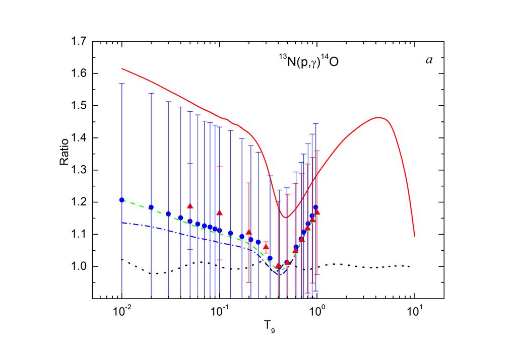
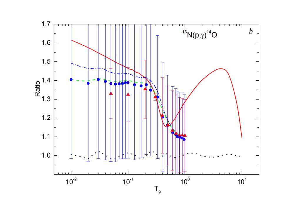
Figure 5: (Color online) The dependence of the ratio of the reaction rates on temperature. $a$) The ratio of the reaction rate obtained in the present calculations and given in Refs. 16 ; 18 ; 23 ; 24 ; 25 , correspondingly : NACRE II 24 - solid curve, Li, et al. 16 - dash-dotted curve, Guo, et al. 27 - dashed curve, Tang, et al. 18 - circles with error bars, Magnus, et al. 23 - triangles with error bars, the dotted curve is the ratio of the estimated speed to its approximation (24); $b$) The ratio of the reaction rates obtained in the present calculations, Refs. 16 ; 18 ; 23 ; 25 to the NACRE II 24 approximated with parameters from Table 4: present calculations - solid curve, Li, et al. 16 - dashed curve, Guo, et al. 27 - dash-dotted curve, Tang, et al. 18 - circles with error bars, Magnus, et al. 23 - triangles with error bars, correspondingly. The dotted curve corresponds to the ratio of NACRE II data and its approximation using the parameters from Table 4.

VI CNO AND HOT CNO CYCLES

Since the late 1930s, when von Weizsäcker Weizsacker and Bethe Bethe independently proposed sets of fusion reactions by which stars convert hydrogen to helium, it is well established that the carbon-nitrogen-oxygen cycles is a mechanism for hydrogen burning in stars. The dominant sequence of reactions for this cycle is the following

$${}^{12}\text{C}(p,\gamma)^{13}\text{N(}e^{+}\nu_{e})^{13}\text{C}(p,\gamma)^{14}\text{N(}p,\gamma)^{15}\text{O(}e^{+}\nu_{e})^{15}\text{N(}p,\alpha)^{12}\text{C.}$$ (25)

The character of the nuclear burning is extremely temperature sensitive and, when temperature is low enough, the hot carbon-nitrogen-oxygen cycle 

$${}^{12}\text{C}(p,\gamma)^{13}\text{N(}p,\gamma)^{14}\text{O}(e^{+}\nu_{e})^{14}\text{N(}p,\gamma)^{15}\text{O(}e^{+}\nu_{e})^{15}\text{N(}p,\alpha)^{12}\text{C}$$ (26)

starts. Since, at low $T_{9}$ temperatures the ¹³N($p,\gamma)^{14}$O reaction in the sequence (26) is competitive with the ¹³N($e^{+}\nu_{e})^{13}$C decay in the sequence (25), the formation and decay of ¹⁴O becomes a major distinguishing feature of this higher temperature cycle. Therefore, the stellar ¹³N($p,\gamma)^{14}$O reaction rate determines the order and the precise temperature of the conversion of the cold CNO cycle to the HCNO cycle and the waiting point in the cycle changes from ¹⁴N to the ¹⁴O and ¹⁵O and the ¹³N($p,\gamma)^{14}$O reaction is a key process which determines this conversion.

One can say that the topic is hardly new, which is illustrated by the number of references on the $S$-factor of the ¹³N($p,\gamma$)¹⁴O reaction and the different reactions rates 16 ; 17 ; 23 ; 26 ; 18 ; 25 . In Ref. Smith it was suggested the most consistent and accurate methodology for analyses of the temperature and density conditions for the HCNO cycle. Below we use this methodology along with our results for the ¹³N($p,\gamma$)¹⁴O reaction rate and reanalyze the dependence of the lifetime against hydrogen burning via ¹³N($p,\gamma$)¹⁴O reaction as a function of temperature and find the temperature window and densities of a stellar medium at which the CNO cycle is converted to the hot CNO cycle. The reanalysis is extended for the stellar density dependence on temperature. Therefore, we use our results for the ¹³N($p,\gamma)^{14}$O reaction rate, follow Ref. Smith and find the temperature window and densities of a stellar medium at which the CNO cycle is converted to the hot CNO cycle. We can achieve the latter by comparing the ¹³N($p,\gamma)^{14}$O, ¹⁴N($p,\gamma)^{15}$O and ¹²C$(p,\gamma)^{13}$N reaction rates and the lifetime of nuclei against destruction by hydrogen burning.

The lifetime of isotopes in the stellar CNO cycle relative to the combustion of hydrogen one can determine as follows Rolfs1988 ; Ryan

$$\tau=\frac{A_{H}}{\rho X_{H}}\frac{1}{N_{A}\left\langle\sigma_{c}v\right\rangle},$$ (27)

where $A_{H}$ is the atomic mass of hydrogen, $X_{H}$ is the relative abundance of hydrogen by mass, $\rho$ is the density of the stellar medium, and $N_{A}\left\langle\sigma_{c}v\right\rangle$ is the appropriate proton-capture reaction rate. Thus, as it is follows from Eq. (27), lifetime is determined precisely by the rate of the corresponding reaction. In our calculations we use the ¹²C$(p,\gamma)^{13}$N, ¹³N($p,\gamma)^{14}$O, and ¹⁴N($p,\gamma)^{15}$O reactions rates. In Fig. 6 the reaction rates of the ¹³ N($p,\gamma)^{14}$O, ¹⁴N($p,\gamma)^{15}$O and ¹²C$(p,\gamma)^{13}$N processes are shown, which are further used in the calculations of $\tau$. For the ¹³N($p,\gamma)^{14}$O reaction we use results of the present calculations and data from Ref. Smith , for the reaction ¹⁴N($p,\gamma)^{15}$O data 29 and Dubovichenko2020 are used, while for the ¹²C$(p,\gamma)^{13}$N we employed data 29 , which are very close to data given in the NACRE II database 24 . Let us comment on the difference in the data for the ¹⁴N($p,\gamma)^{15}$O reaction (curves 3 and 5 in Fig. 6). In contrast to Ref. 29 , in Ref. Dubovichenko2020 the ¹⁴N($p,\gamma)^{15}$O reaction rate was calculated by taking into account radiative capture of protons both in the GS of ¹⁴N nucleus and in all four excited bound levels. Such consideration allows one to describe experimental data for the astrophysical $S$-factors of the radiative proton capture on ¹⁴N to five excited states of the ¹⁵O nucleus at the excitation energies from 5.18 MeV to 6.86 MeV under the assumption, that all five resonances are $D$ scattering waves. The latter approach leads to a significant increase of the ¹⁴N($p,\gamma)^{15}$O reaction rate at temperatures $T_{9}>0.3$, which is indicated in Fig. 6.

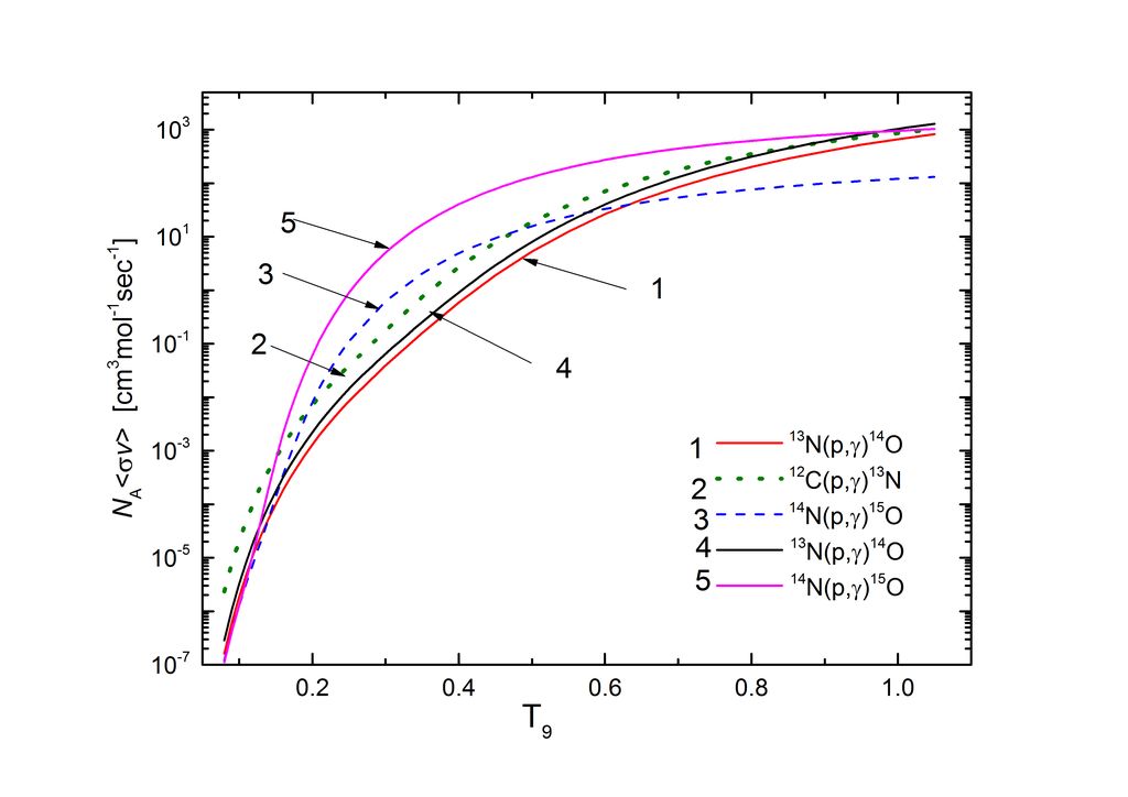
Figure 6: (Color online) The dependence of the reaction rates $N_{A}\left\langle\sigma_{c}v\right\rangle$ on temperature for the ¹²C$(p,\gamma)^{13}$N, ¹³N($p,\gamma)^{14}$O, and ¹⁴N($p,\gamma)^{15}$O reactions. Curves: 1, 2 and 3 - the data are taken from Ref. Smith , 4 - present calculation, 5 - results from Ref. Dubovichenko2020 .

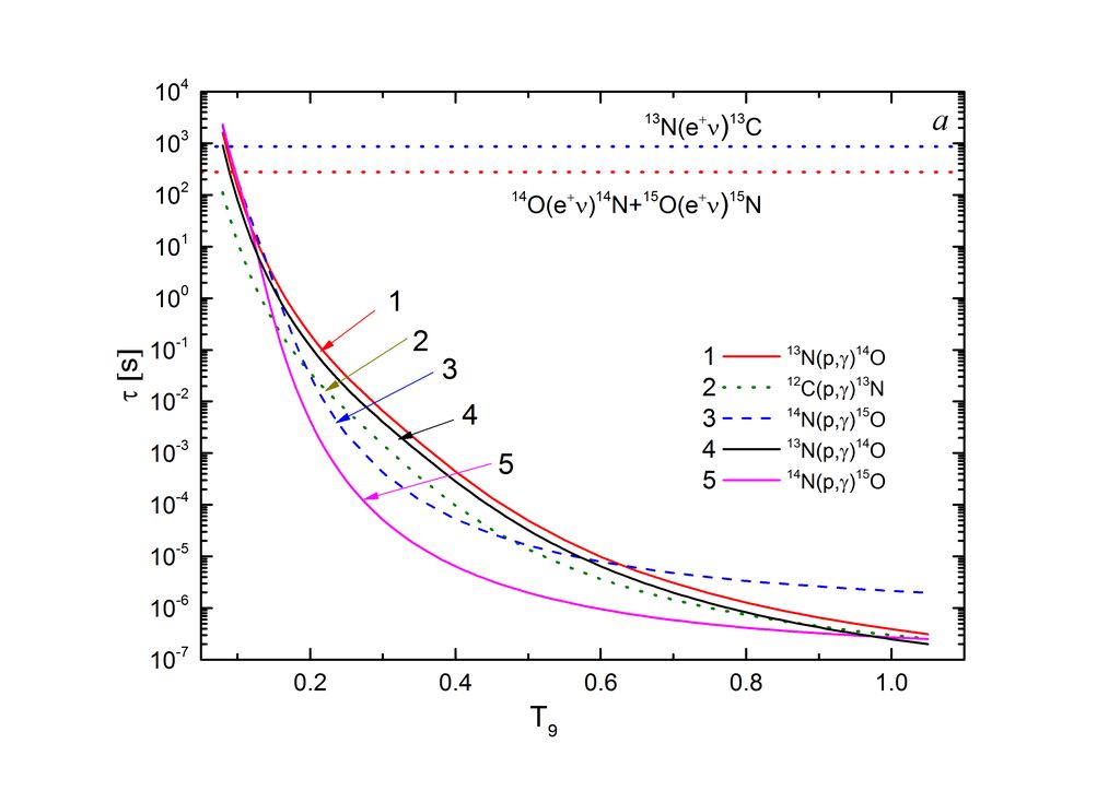
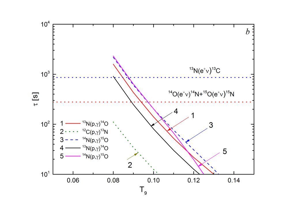
Figure 7: (Color online) Comparison of lifetime against hydrogen burning via the ¹²C$(p,\gamma)^{13}$N, ¹³N($p,\gamma)^{14}$O, and ¹⁴N($p,\gamma)^{15}$O reactions as a function of temperature, and the ¹³N, ¹⁴O, and ¹⁵O $\beta$- decay lifetimes for the temperature intervals ($a$) $0.08<T_{9}<1.0$ and ($b$) $0.08<T_{9}<0.14$.

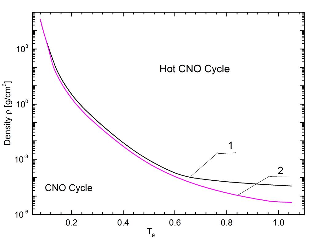
Figure 8: (Color online) Density and temperature range for the operation of the hot CNO cycle. Curves: 1 - result from Ref. Smith ; 2 - present result.

In order to determine the astrophysical temperatures at which the CNO cycle is converted to the HCNO cycle, it is necessary to determine the ¹³N($p,\gamma)^{14}$O reaction rate as a function of temperature and compare it with one for the other processes. Using the reaction rates presented in Fig. 6, we calculate the dependence of the lifetime of isotopes produced in the processes ¹²C$(p,\gamma)^{13}$N, ¹³N($p,\gamma)^{14}$O, and ¹⁴N($p,\gamma)^{15}$O on temperature. Following Ref. Smith , in calculations we used for the hydrogen mass fraction $X_{H}=0.77$ and the stellar density $\rho=5\times 10^{3}$ g/cm³ Wiescher1986 .

The dependencies of the lifetime of isotopes produced in the processes on the temperature are presented in Fig. 7. The data for the lifetime of radioactive isotopes are also presented in Fig. 7: $\tau_{{}^{13}\text{N}}$ $=863$ s for the ¹³N($e^{+}\nu_{e})^{13}$C, $\tau_{{}^{14}\text{O}}$ $=$ 102 s for the ¹⁴O$(e^{+}\nu_{e})^{14}$N and $\tau_{{}^{15}\text{O}}$ $=$176 s for the ¹⁵O($e^{+}\nu_{e})^{15}$N. The analysis of the results presented in Fig. 7 shows that at $T_{9}=$0.08 the ¹³N($p,\gamma)^{14}$O and ¹³N($e^{+}\nu_{e})^{13}$C reactions have equal lifetime. When the lifetime of ¹⁴O isotope produced via ¹³N($p,\gamma)^{14}$O reaction will be less than the ¹³N($e^{+}\nu_{e})^{13}$C decay lifetime, the reaction sequence changes to the hot CNO cycle. For these conditions in CNO cycle the lifetimes of the $\beta^{+}$-unstable systems such as ¹³N and ¹⁵O are long enough that proton capture can occur on these unstable nuclei before they undergo the $\beta^{+}$-decay.

The onset of the HCNO cycle occurs at $T_{9}=$0.08 when the rate of the slowest ¹³N($p,\gamma)^{14}$O reaction exceeds the ¹⁴O$(e^{+}\nu_{e})^{14}$N and ¹⁵O($e^{+}\nu_{e})^{15}$N decay rates. Moreover, at $T_{9}=0.1$ the ratio of the ¹³N($p,\gamma)^{14}$O and ¹³N($e^{+}\nu_{e})^{13}$C rates is 10.8, in the contract to Ref. Smith , where this ratio is about 6. Therefore, at $T_{9}=0.1$ the reaction ¹³N($p,\gamma)^{14}$O is already ten times faster than the ¹³N($e^{+}\nu_{e})^{13}$C decay, resulting in the mass flow going via ¹⁴O at the very onset of the HCNO cycle. The present result indicates that the HCNO cycle is turned on at the early stage of a nova explosion when the temperature is lower than reported in the earlier calculations 27 and Smith .

Our calculations lead to the temperature range $0.13<T_{9}<0.97$, where the reaction rate of ¹⁴N($p,\gamma)^{15}$O is greater than the reaction rate of ¹³N($p,\gamma)^{14}$O. The ¹³N($p,\gamma)^{14}$O reaction rate obtained in the present calculations leads to the temperature window which is much wider than reported in Ref. Smith : $0.14<T_{9}<0.64.$ One should mention that the reaction rates for ¹³N($p,\gamma)^{14}$O in the present work and ¹⁴N($p,\gamma)^{15}$O Dubovichenko2020 are obtained in the framework of the same theoretical approach.

Following Ref. Smith , let’s determine the dependence of the stellar medium density corresponding to the onset of the HCNO cycle on temperature as

$$\rho=\frac{A_{H}}{X_{H}(\tau_{{}^{14}\text{N}}+\tau_{{}^{15}\text{N}})}\frac{1}{N_{A}\left\langle\sigma_{c}v\right\rangle_{\min}},$$ (28)

where the smallest reaction rate $N_{A}\left\langle\sigma_{c}v\right\rangle_{\min}$ includes the temperature dependence. An analysis of the density-temperature relationship allows to determine the temperatures and densities at which the stellar CNO cycle is converted to the HCNO cycle. If the density and temperature of the stellar medium fall above the curve $\rho(T)$ on the density-temperature diagram, then HCNO cycle occurs, otherwise the CNO cycle operates.

The results of present calculations for the density-temperature dependence $\rho(T)$ along with results from Ref. Smith are shown in Fig. 8. The comparison of our calculations and results Smith indicates that at the same temperature range HCNO cycle operates at the lower densities of a stellar medium than in the case reported in Smith . Analysis of the results given at the density-temperature diagram in Fig. 8 demonstrate that at an early stage of a nova explosion at the temperature range $0.2$ $T_{9}-0.4$ $T_{9}$ the hot CNO cycle could be turned on at a twice less density of the stellar matter. The difference becomes more significant at $T_{9}>0.6$ and the HCNO cycle could be operated when at $1$ $T_{9}$ a stellar medium density becomes about 10 times less compared to Smith , as can be seen from Fig. 8.

Reanalysis of the astrophysical S-factor and reaction rate of the proton capture on ¹³N nucleus leads us to the numerical differences with previous studies. These numerical differences bring us to a new temperature corridor for the conversion of stellar CNO cycle to the HCNO cycle. The small variation for the range of the HCNO window may lead to the huge macroscopic consequences on the scale of astrophysical events. Thus, in supermassive stars at high temperature the ignition of the hot CNO cycle can occur at much lower densities, generating sufficient energy which can affect very massive stars collapse at the end of their life cycle.

VII Conclusion

We briefly summarize our results. We have employed the modified potential cluster model to describe the ¹³N($p,\gamma$)¹⁴O reaction at astrophysical energies and influence of the first $p^{13}$N resonance width on the astrophysical $S$-factor. At energies of 30–70 keV, the $S$-factor remains almost constant with the average value 8.4(2) keV$\cdot$b, thereby determining its value at zero energy, which is determined by the potential of the $S$-wave scattering. The values of $S(0)$-factor of 7.0(2) to 8.4(2) keV$\cdot$b are listed in Table 1 for three options of potentials, which correspond to three different values of energies for resonance in the $S$ scattering wave. The potentials of the $S$-wave, leading to the correct resonance width for different resonance energies, do not allow us to obtain the value of the $S$-factor, which would be consistent with previous results. Only a decrease in the resonance width to 22–26 keV leads to the $S$-factor of the order of 5 keV$\cdot$b, which is consistent with the upper limit of the results from 24 and the results of other works, for example, 17 ; 18 ; 25 . Thus, an accurate determination of the width is crucial. Our results demonstrate that contributions of the $M1$ and $E2$ transitions in the $S$-factor are negligible at energies $E<1$ MeV, but are significant at high energies. At the resonance energy, the $S$-factor reaches 2.4 MeV$\cdot$b, which is in a good agreement with the results of previous studies. Using the MPCM capabilities, it was shown that the values of the astrophysical $S$-factor of the ¹³N($p,\gamma)^{14}$O reaction at ultralow energies strongly depends on the ${}^{3}S_{1}$ resonance parameters.

Based on the potentials for the $S$ scattering wave, consistent with the energy and widths of the first resonance, the ¹³N($p,\gamma$)¹⁴O reaction rate was calculated and a simple analytical approximation for the reaction rate was proposed. The inclusion of resonances at 1.981, 3.117, and 5.123 MeV practically does not affect the reaction rate, although, the contributions of resonances are clearly visible when calculating the $S$-factor. The reason for such a weak influence is their small widths and relatively large resonance energies. Results of our calculations for the ¹³N($p,\gamma)^{14}$O reaction rate provide the contribution to the steadily improving reaction rate libraries.

A precise knowledge of a cross section of the radiative proton capture on ¹³N isotope at the low energy is important as it plays a key role in the HCNO cycle, due to the proton capture rate on ¹³N at temperature range of 0.05 $T_{9}-1.0$ $T_{9}$ can become of the same order or larger than the ¹³N($e^{+}\nu_{e})^{13}$C decay rate. Our calculations show that at $T_{9}=0.1$ the ratio of the ¹³N($p,\gamma)^{14}$O and ¹³N($e^{+}\nu_{e})^{13}$C rates is 10.8.

In the context of the CNO cycle scenario, our calculations of the ¹³N($p,\gamma)^{14}$O and results for the other bottleneck ¹⁴N($p,\gamma)^{15}$O reaction Dubovichenko2020 together with the NACRE II data 24 for the ¹²C$(p,\gamma)^{13}$N process show that in the temperature window $0.13<T_{9}<0.97$, where the reaction rate of ¹⁴N($p,\gamma)^{15}$O is greater than the reaction rate of ¹³N($p,\gamma)^{14}$O, occurs the conversion of the CNO cycle to the HCNO cycle. The present result indicates that the HCNO cycle is turned on at the early stage of a nova explosion at temperature $T_{9}=$0.08. Therefore, the significant mass flow through ¹⁴O nucleus begins to occur at temperature $T_{9}=0.08$. Our calculations show that at this temperature the ¹³N($p,\gamma)^{14}$O reaction rate and the decay rate of the ¹³N($e^{+}\nu_{e})^{13}$C process are equal.

Our results demonstrate that at early stages of a nova explosion at temperatures about $0.1$ $T_{9}$ and at late stages of evolution of supermassive stars at temperatures about $1$ $T_{9}$ the ignition of the hot CNO cycle could occur at much lower densities of a stellar medium.

Therefore, at temperature and density of a stellar medium such as the conditions in a nova explosion and very massive stars hydrogen burning occurs at temperatures $0.01$ $T_{9}-1.0$ $T_{9}.$ For these conditions in CNO cycle the lifetimes of the $\beta^{+}$-unstable systems such as ¹³N and ¹⁵O are long enough that proton capture can occur on these unstable nuclei before they undergo the $\beta^{+}$-decay.

Acknowledgement

This work was supported by a grant from the Ministry of Education and Science of the Republic of Kazakhstan under the program # BR05236322 “Investigations of physical processes in extragalactic and galactic objects and their subsystems” under the theme “Study of thermonuclear processes in stars and primary nucleosynthesis of the Universe” through the name of Fesenkov Astrophysical Institute of the National Center for Space Research and Technology of the Ministry of Digital Development, Innovation and Aerospace Industry of the Republic of Kazakhstan

References

- (1) E. Wiescher, J. Görres, E. Uberseder, G. Imbriani, and M. Pignatari, Ann. Rev. Nucl. Part. Sci. 60, 381 (2010).
- (2) M. Wiescher, F. Käppeler, and K. Langanke, Ann. Rev. Astron. Astrophys. 50, 165 (2012).
- (3) C. R. Brune and B. Davids, Ann. Rev. Nucl. Part. Sci. 65, 87 (2015).
- (4) M. Wiescher, et al., Nucl. Phys. A 349, 165 (1980).
- (5) C. A. Bertulani, A. Gade, Phys. Rep. 485, 195 (2010).
- (6) P. Decrock, Th. Delbar, P. Duhamel, W. Galster, M. Huyse, P. Leleux, I. Licot, et al., Phys. Rev. Lett. 67, 808 (1991).
- (7) P. Decrock, M. Gaelens, M. Huyse, G. Reusen, G. Vancraeynest, P. Van Duppen, et al., Phys. Rev. C 48, 2057 (1993).
- (8) Th. Delbar, W. Galster, P. Leleux, I. Licot, E. Lienard, P. Lipnik, et al., Phys. Rev. C 48, 3088 (1993).
- (9) T.E. Chupp, R.T. Kouzes, A.B. McDonald, P.D. Parker, T.F. Wang, A. Howard, Phys Rev. C 31, 1023 (1985).
- (10) P. B. Fernandez, E. G. Adelberger, A. Garcia, Phys. Rev. C 40, 1887 (1989).
- (11) M. S. Smith, P. V. Magnus, K. I. Hahn, R. M. Curley, P. D. Parker, T. F. Wang, et al., Phys. Rev. C 47, 2740 (1993).
- (12) T. Motobayashi et al., Phys. Lett. B 624, 259 (1991).
- (13) J. Kiener et al., Nucl. Phys. A 552, 66 (1993).
- (14) G. Baur and H. Rebel, J. Phys. G. 20, 1 (1994).
- (15) Z. H. Li et al., Phys. Rev. C 74, 035801 (2006).
- (16) W. Liu et al., Int. J. Mod. Phys. E 15, 1899 (2006).
- (17) R. J. Charity, K. W. Brown, J. Okolowicz, M. Ploszajczak, J. M. Elson, W. Reviol et al., Phys. Rev. C 100, 064305 (2019).
- (18) P. V. Magnus, E.G. Adelberger, A. Garcia, Phys. Rev. C 49, R1755 (1994).
- (19) G. J. Mathews and F. S. Dietrich, Astrophys. J. 287, 969 (1984).
- (20) K. Langanke, O. S. Van Rogsmalen and W. A. Fowler, Nucl. Phys. A 435, 657 (1985).
- (21) C. Funck and K. Langanke, Nucl. Phys. A 464, 90 (1987).
- (22) X. Tang, A. Azhari, C. Fu, C. A. Gagliardi, A. M. Mukhamedzhanov, F. Pirlepesov, L. Trache, et al., Phys. Rev. C 69, 055807 (2004).
- (23) X. Tang et al., Phys. Rev. C 67, 015804 (2003).
- (24) B. Guo and Z. H. Li, Chin. Phys. Lett. 24, 65 (2007).
- (25) J. T. Huang, C. A. Bertulani, V. Guimarães, Atomic Data and Nuclear Data Tables 96, 824 (2010).
- (26) C. Angulo et al., Nucl. Phys. A 656, 3 (1999).
- (27) Y. Xu, K. Takahashi, S. Goriely et al., Nucl. Phys. A 918, 169 (2013).
- (28) F. Ajzenberg-Selove, Nucl. Phys. A 523, 1 (1991).
- (29) S. I. Sukhoruchkin and Z. N. Soroko, Excited nuclear states, Sub. G. Suppl. I/25 A-F. Springer, (2016).
- (30) S. B. Dubovichenko, Thermonuclear processes in Stars and Universe. Second English ed., expanded and corrected. Germany, Saarbrucken: Scholar’s Press. 2015.
- (31) M. Wiescher and T. Ahn, Clusters in Astrophysics, in “Nuclear Particle Correlations and Cluster Physics”, Chap. 8, Ed. Wolf-Udo Schröder, World Scientific, pp. 203-255, 2017.
- (32) S. B. Dubovichenko, Radiative Neutron Capture, Walter de Gruyter GmbH, Berlin/Boston, 296 p. (2019).
- (33) S. B. Dubovichenko, A. V. Dzhazairov-Kakhramanov, Nucl. Phys. A 941, 335–363 (2015).
- (34) S. B. Dubovichenko, N. A. Burkova, A. V. Dzhazairov-Kakhramanov, R. Ya. Kezerashvili, Ch. T. Omarov, A. S. Tkachenko, and D. M. Zazulin, Nucl. Phys. A 987, 46 (2019).
- (35) S. B. Dubovichenko, N. A. Burkova, and A. V. Dzhazairov-Kakhramanov, Int. J. Mod. Phys. 29, 1930007 (2020).
- (36) C. A. Barnes, D. D. Clayton, D. N. Schramm, Essays in Nuclear Astrophysics. Presented to William A. Fowler. UK, Cambridge: Cambridge University Press. 562p. 1982.
- (37) V. G. Neudatchin, V. I. Kukulin, V. N. Pomerantsev, and A. A. Sakharuk, Phys. Rev. C 45, 1512 (1992).
- (38) O. F. Nemets, V. G. Neudatchin, A. T. Rudchik, Yu. F. Smirnov, Yu. M. Tchuvil’sky, Nucleon association in atomic nuclei and the nuclear reactions of the many nucleons transfers. Kiev: Naukova Dumka. 488p. 1988. (in Russian).
- (39) K. Wildermuth and Y. C. Tang, A unified theory of the nucleus. Braunschweig: Vieweg. 498p., 1977.
- (40) Y. C. Tang, M. LeMere, and D. R. Thompsom, Phys. Rep. 47, 167 (1978).
- (41) https://physics.nist.gov/cgi-bin/cuu/Value?mudjsearch2520for=atomnuc!
- (42) http://cdfe.sinp.msu.ru/services/ground/NuclChart_release.html
- (43) F. Nichitiu, Phase shifts analysis in physics. Romania: Acad. Publ. 416 p. (1980).
- (44) S. B. Dubovichenko, A. V. Dzhazairov-Kakhramanov, Rus. Phys. J. 52, 833 (2009).
- (45) V. G. Neudatchin and Yu.F. Smirnov, Nucleon associations in light nuclei. Moscow: Nauka. 414p. 1969. (in Russian).
- (46) V. I. Kukulin, V. G. Neudatchin, Yu. F. Smirnov, Nucl. Phys. A. 245, 429 (1975).
- (47) C. Itzykson, M. Nauenberg, Rev. Mod. Phys. 38, 95 (1966).
- (48) D. A. Varshalovich, A. N. Moskalev, V. K. Khersonski, Quantum theory of angular momemtum, World Scientific. 514p., 1988.
- (49) A. S. Tkachenko, R. Ya. Kezerashvilic, N. A. Burkova, S. B. Dubovichenko, Nucl. Phys. A 991, 121609 (2019).
- (50) E. M. Tursunov, S. A. Turakulov, P. Descouvemont, Phys. Atom. Nucl. 78, 193 (2015).
- (51) F. Hammache et al., Phys. Rev. C 82, 065803 (2010).
- (52) W. A. Fowler, G. R. Caughlan, and B. A. Zimmerman, Ann. Rev. Astron. Astrophys. 5, 525 (1967).
- (53) A. M. Mukhamedzhanov et al., Nucl. Phys. A 725, 279 (2003).
- (54) G. R. Plattner, R. D. Viollier, Coupling constants of commonly used nuclear probes, Nucl. Phys. A 365, 8 (1981).
- (55) D. Baye and E. Brainis, Phys. Rev. C 61, 025801 (2000).
- (56) S. G. Ryan and A. J. Norton, Stellar evolution and nucleosynthesis, Campridge University Press, New York, 240 p. 2010.
- (57) http://cdfe.sinp.msu.ru/exfor/index.php.
- (58) G. R. Caughlan and W. A. Fowler, Atom. Data Nucl. Data Tab. 40, 283 (1988).
- (59) C. F. von Weizsäcker, Physikalische Zeitschrift. 38, 176 (1937).
- (60) H. A. Bethe, Phys. Rev. 55, 103 (1939).
- (61) C. Rolfs and W. S. Rodney, Cauldrons in the Cosmos, University of Chicago Press, Chicago, 1988.
- (62) M. Wiescher, J. Gorres, F. -K. Thielemann, and H. Ritter, Astron. Astrophys. 160, 56 (1986).