Using Machine Learning to predict extreme events in the Hénon map

Abstract

Machine Learning (ML) inspired algorithms provide a flexible set of tools for analyzing and forecasting chaotic dynamical systems. We here analyze the performance of one algorithm for the prediction of extreme events in the two-dimensional Hénon map at the classical parameters. The task is to determine whether a trajectory will exceed a threshold after a set number of time steps into the future. This task has a geometric interpretation within the dynamics of the Hénon map, which we use to gauge the performance of the neural networks that are used in this work. We analyze the dependence of the success rate of the ML models on the prediction time $T$, the number of training samples $N_{T}$ and the size of the network $N_{p}$. We observe that in order to maintain a certain accuracy, $N_{T}\propto\exp(2hT)$ and $N_{p}\propto\exp(hT)$, where $h$ is the topological entropy. Similar relations between the intrinsic chaotic properties of the dynamics and ML parameters might be observable in other systems as well.

The power of ML algorithms in the handling of complex tasks is impressively demonstrated by their successes in the game of Go Silver et al. (2017) and real world applications from pattern recognition to autonomous driving. Within physics, they are used to select suitable bases for many body quantum systems Schuld et al. (2019), to classify patterns and phases in many body systems Jeckel et al. (2019) or phase transitions in material science Carrasquilla and Melko (2017); Butler et al. (2018), and to derive low-dimensional models for turbulent flows Brunton et al. (2019) and other systems Champion et al. (2019), to mention just a few. In chaotic systems, time series prediction is challenging because of the sensitive dependence on initial conditions and the ensuing increase in uncertainty Ott (2002). We here analyze the performance of a particular class of ML algorithms for predicting extreme events in the Hénon map, as a model for similar tasks in other systems.

I Introduction

Machine Learning (ML) algorithms emerge as a flexible and versatile tool for the analysis and the characterization of complex systems. Following the initial applications of neural networks for the prediction of a wide range of physical and non-physical time series Weigend et al. (1990); Mukherjee et al. (1997); Bontempi et al. (2013), interest in ML has been revived by the impressive demonstration of the representation and prediction of a spatially-extended Kuramoto-Shivashinsky system by Ott and collaborators Pathak et al. (2018). They have also shown, how the dynamics of a trained network can be used to extract the Lyapunov exponents for the original system from the Lyapunov exponent of the network Pathak et al. (2017). As prediction is a common task in many situations, including targeting satellites, forecasting weather Lorenz (1963) or stock markets, ML learning tools hold great potential because of their apparently high adaptability despite rather simple design principles. However, there are numerous parameters that influence the power of the networks, including the number of training samples, the time interval over which a prediction is requested, or the topology of the network. Our aim here is to analyze the effect of some of these parameters.

The task we use to gauge the power of ML algorithms is guided by considerations in transitional shear flows: experimental, numerical and theoretical results show that in parameter ranges intermediate between laminar and fully developed turbulent, the turbulent states are not persistent but transient Hof et al. (2006). The decay is memoryless, and happens without any noticeable precursor. Nevertheless, decaying trajectories have to depart from the turbulent saddle at some point, and the identification of when and where this happens can be useful for manipulations of the turbulent dynamics and the understanding of the turbulent saddle itself (see, e.g. Eckhardt et al. (2007); Eckhardt (2018)). Here we rephrase the decay prediction problem as a task in the Hénon map, and leave the application to the relaminarization problem (see Schlatter et al Srinivasan et al. (2019) for an example) for a future publication.

We use the two-dimensional (2d) Hénon map as dynamical system and pose a task that has a geometric interpretation in the state space of the system: the task is to predict whether a trajectory that starts at a certain point in state space will pass a prescribed threshold $\theta$ after $T$ iterations. In relation to the relaminarization problem in transient turbulent flows, the threshold corresponds to a barrier beyond which the flow becomes laminar. When reduced to two dimensions and a map, the task becomes much easier to analyze, while at the same time keeping the essential dynamical features of the flow: the Lyapunov exponent is positive, the task becomes more challenging with increasing time, and it depends on ever finer details of the initial conditions.

The outline of the paper is as follows. In section 2 we describe the Hénon map and the geometrical interpretation of the task. In section 3, we discuss the training of the network and its dependence on three critical parameters: the number of training samples $N_{T}$, the forecasting time $T$, and the number of parameters $N_{p}$ in the neural network used for the task. We conclude with a few observations and general remarks in section 5 after presenting the results in section 4.

II Thresholds in the Hénon map

The Hénon map Hénon (1976) is a two dimensional discrete non-linear map,

$$\begin{split}x_{n+1}&=1-ax_{n}^{2}+y_{n}\\ y_{n+1}&=bx_{n}.\end{split}$$ (1)

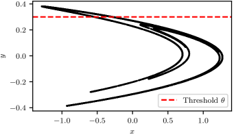
with two parameters $a$ and $b$. For the common choice of $a=1.4$ and $b=0.3$, the dynamics is chaotic with a positive Lyapunov exponent, and a positive topological entropy $h=0.465$ Artuso et al. (1990). Equation (1) can be written as a one dimensional discrete non-linear map that depends on the two preceding iterates, $z_{n+1}=1-az_{n}^{2}+bz_{n-1}$. However, the two dimensional Hénon map formulation is used here. The familiar shape of the attractor with the threshold is shown in Fig. 1. The threshold for the $y$ coordinate is set at $\theta=0.3$ and is kept fixed for all studies presented here: while other values will give changes in detail, we do not expect any substantial changes in the general conclusions we draw here.

Figure 1: The Hénon attractor in state space. Points on the Hénon attractor are shown as black dots and the dashed red line denotes the threshold $\theta$ that is used for the prediction task in Eq. (3).

The prediction task on the chaotic attractor is defined as follows: Given as input a set of phase space points $(x_{i},y_{i})$ where $i=n$, $n-1$, $n-2$, …, $n-(N-1)$, i.e. the phase space point at time $n$ and its predecessors down to $n-(N-1)$ for a total of $N$ points,

$$\{(x_{i},y_{i})\}_{i=n-(N-1),\dots,n},$$ (2)

predict whether the macroscopic criterion

$$y_{n+T}\geq\theta=0.3$$ (3)

is fulfilled at a point in time that is $T$ steps in the future. Note that we do not ask whether the threshold is passed at intermediate times: while this may be relevant for the decay problem of turbulence, numerical results show that the main effect of this change is to fragment the state space even more. The particular choice of $\theta$ is arbitrary, and a range of values will give similar results. For finite $T$, the points that pass the threshold vary continuously with $\theta$ so that the results will be robust under variations with $\theta$. For increasing times the range in $\theta$ for which this remains true decreases, and eventually discontinuous changes in the regions in which the criterion is satisfied will appear.

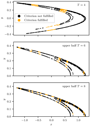
Equation (3) resembles a macroscopic criterion in a chaotic trajectory and is motivated by the criterion we usually use in the determination of turbulent lifetimes: trajectories decay when the energy content in transverse modes falls below a critical value Schneider and Eckhardt (2009), here replaced by a trajectory reaching $y\geq\theta$. The regions that satisfy the criterion are shown in Fig. 2: The initial conditions that will pass the threshold after $T$ time steps come from compact regions in the phase space that increase in number and become smaller in diameter as $T$ increases.

Figure 2: Points on the attractor that pass the threshold after $T$ steps for $T=4$ (top), $T=6$ (middle) and $T=8$ (bottom). Points on the attractor that are above the threshold are shown in orange, those below in black. To better demonstrate the small regions for larger $T$, the middle and bottom frame only show the upper half $y\geq 0$ of the state space.

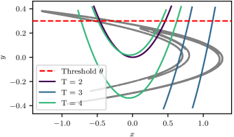
The regions that satisfy the criterion (3) after $T$ iterations have a geometrical interpretation, obtained by considering the preimages of the threshold, i.e. by asking which points end up on the threshold after $n$ steps. To start, the preimages of a point $(x_{n+1},y_{n+1})$ are determined by the inverse of the map,

$$\begin{split}x_{n}&=\frac{y_{n+1}}{b}\\ y_{n}&=x_{n+1}-1+a\frac{y_{n+1}^{2}}{b^{2}}.\end{split}$$ (4)

Specifically, the line $y_{n+1}=\theta$ has as a preimage the line

$$\begin{split}x_{n}&=\frac{\theta}{b}\\ y_{n}&=x_{n+1}-1+a\frac{\theta^{2}}{b^{2}}.\end{split}$$ (5)

Everything to the right of $x_{n}=\theta/b$ will be mapped above $y_{n+1}=\theta$. Going one more step into the past, the line $(x_{n}=\theta/b,y_{n})$ will be mapped to the parabola

$$\begin{split}x_{n-1}&=\frac{y_{n}}{b}\\ y_{n-1}&=\frac{\theta}{b}-1+a\frac{y_{n}^{2}}{b^{2}}.\end{split}$$ (6)

All points inside the parabola will be mapped above $y_{n+1}=\theta$ in two steps. Iterating further into the past, the pre-images become more convoluted, as indicated in Fig. 3. As the number of time steps into the past increases, the preimages of the threshold develop more and more lines that cross the attractor, each one of them dividing the attractor into ever smaller segments that will be mapped above $y_{n}$ for some time steps into the future.

Figure 3: Inverse iterates of the threshold. The gray points show the Hénon attractor and the red line marks the threshold of the criterion (3). Preimages of the threshold become more complex as the number of time steps $T$ into the past increases, as initially connected phase space regions are split up into subsets. The preimages of the threshold develop ever more folds that cut the Hénon attractor.

III Machine learning for predictions

We now turn to the application of ML tools for the prediction task. The prediction task formulated in the last preceeding section is considered a classification task in the ML literature Goodfellow et al. (2016). The neural network that is used as ML model in this work is trained to classify a given sample to belong to one of the two classes separated by the criterion Eq. (3). Consequently, the regions which make up the geometrical task interpretation in Fig. 2 are considered classes in the ML parlance. One class are the phase space points colored in orange in Fig. 2 that fulfill Eq. (3) and the other class are the phase space points colored in black, which do not fulfill (3).

Among the many possible network topologies and neural dynamics, we use a fully connected feed forward neural network.

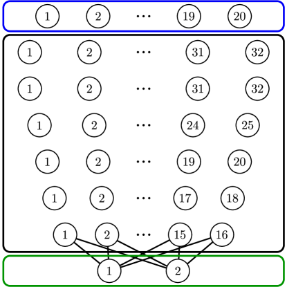
The latter is a directed acyclic graph that is made up of layers, as shown schematically in Fig. 5. The interactions between the layers $i-1$ and $i$ are computed by applying an activation function $g$ to the latent variable $\bm{z}^{(i)}$, which itself is a linear function of the previous layer $\bm{y}^{(i-1)}$,

$$\begin{split}\bm{z}^{(i)}&=\bm{W}^{(i,i-1)}\cdot\bm{y}^{(i-1)}\\ \bm{y}^{(i)}&=g(\bm{z}^{(i)}).\end{split}$$ (7)

The weight matrix $\bm{W}^{(i,i-1)}$ connects the neurons of layer $i-1$ stored in $\bm{y}^{(i-1)}$ to the latent variables of layer $i$ stored in $\bm{z}^{(i)}$. An evaluation of a fully connected feed forward neural network then applies Eq. (7) for each layer in the network, starting from the input layer $i=0$ and ending with the output layer. Feed forward neural networks are trained by adapting all weight matrices summarized into a high dimensional parameter vector $\mathbf{\Gamma}=[\bm{W}^{(i,i-1)}]_{i=1,\dots,n_{l}}$, where $n_{l}$ is the number of layers, in order to minimize a pre-defined loss functional $\mathcal{L}(\mathbf{\Gamma})$.

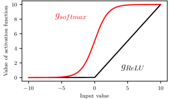
The neural network we use here has $n_{l}=8$ layers, the first layer being the input layer, followed by six hidden layers and a final output layer. ReLU activation functions Goodfellow et al. (2016) are used for the hidden layers and the output layer uses a softmax activation function Goodfellow et al. (2016). These two types of activation functions are shown in Fig. 4. While the details of the results we present will depend on this specific choice, we anticipate that other network topologies or activation functions will show similar behaviour.

Figure 4: Activation functions for hidden and output layers. The ReLU function $ReLU(x)=\max(0,x)$ (black) is used for the hidden layers, and the softmax function (red) for the output layer. Since there are two output classes, the softmax function is equivalent to the sigmoid function, $\sigma(x)=1/(1-e^{-x})$. The softmax function is scaled to the maximal value of $10$ for visual purposes.

With an input based on the current position and $N-1$ further steps into the past, it has dimensions $2N$. Therefore, the number of neurons in the first layer is $2N$, where we work with $N=10$. The numbers of neurons per layer are then taken to be $(2N,32,32,25,20,18,16,2)$, with the number of hidden nodes and the final output node fixed. The output as softmax layer returns two numbers that are often interpreted as probabilities of the input being in the respective classes. The input is then classified according to which of the two numbers is larger. The neural network is shown schematically in Fig. 5. Choosing the specific neural network topology being a heuristic, the first hidden layer is enlarged and subsequent layers follow roughly a linear interpolation down to the output layer, as suggested in Heaton (2008). The topology presented above starts to learn the task by decreasing the loss function value upon training and, hence, has been chosen as baseline topology.

Figure 5: Topology of the neural network. There are $2N$ input nodes (blue box), with $N$ the number of time steps in the past, $(32,32,25,20,18,16)$ hidden layers (black box), with a ReLU activation function, and 2 output neurons (green box) with a softmax activation function. The network is fully connected between layers. Each neuron of the input and hidden layers is connected to every neuron in its subsequent layer. Only the weights of the last hidden layer to the output layer are visualized in order to avoid excess visual load by the large number of weights. The numbers enumerate the neurons in each layer.

Concerning the loss functional, the binary classification problem motivates the usage of the binary categorial cross-entropy Goodfellow et al. (2016) as it is commonly defined in Machine Learning Goodfellow et al. (2016) by

$$\mathcal{L}(\mathbf{\Gamma})=\frac{1}{N_{T}}\sum_{i=1}^{N_{T}}y_{i}\log(p(x_{i},\mathbf{\Gamma}))+(1-y_{i})\log(1-p(x_{i},\mathbf{\Gamma}))$$ (8)

with $N_{T}$ as the number of training samples, $y_{i}$ the true label of training sample $i$, $x_{i}$ the trajectory data of sample $i$ and $p(x_{i},\mathbf{\Gamma})$ the probability of sample $i$ to fulfill criterion (3) as predicted by the neural network with parameters $\mathbf{\Gamma}$. The Adam optimizer Kingma and Ba (2014) is used to minimize $\mathcal{L}$. This optimizer extends the regular stochastic gradient descent optimizer by step size adaptivity per weight and uses past gradient magnitudes of $\mathcal{L}$ to estimate appropriate step sizes. Calculating the gradients of all $N_{T}$ summands is computationally unfeasible. The underlying stochastic gradient descent therefore approximates $\nabla_{\Gamma}\mathcal{L}(\bm{\Gamma})$ by taking $m\ll N_{T}$ random samples from the $N_{T}$ training samples. The quantity $m$ is called batchsize and is here set to $m=128$. The training is performed for $5000$ epochs, where one epoch consists of showing all $N_{T}$ training samples once to the optimizer during the stochastic gradient step.

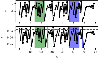
The number of samples $N_{T}$ in the training set is varied from $10^{3}$ to $3\cdot 10^{5}$, as detailed below. The training data is sampled from the natural Hénon dynamics by first iterating Eq. (1) and second including each point’s history according to Eq. (2), see Fig. (6). Finally, the training data are scaled to zero-mean and unit variance. The training labels are determined according to Eq. (3) and $N_{T}/2$ training samples per each of the two classes are used in order to train the network on an equal number of samples per class. This avoids biases in the predictions of the neural network that occur for imbalanced data He and Garcia (2009).

The performance of the network is evaluated by the predictions for a fixed large data set of $10^{6}$ samples that have not been used for training purposes. Also for this test data, we ensure that the number of samples per class is equal for both classes. The percentage of correctly classified samples of this verification corpus is called accuracy and is used as the measure for the performance of the network. An accuracy of $50\%$ is equivalent to random guessing and represents the lower point of reference. An accuracy of $100\%$ corresponds to perfect classification and gives the upper point of reference.

Figure 6: Example trajectory of the Hénon map with explanation of training data construction. The two subplots correspond to the components $x$ and $y$. The black lines with dots are the iterates starting from some initial conditions. The dashed red line marks the threshold of $\theta=0.3$ for the $y$ component that is used for the task definition. Furthermore, two sets of points are colored in green and blue to exemplify how training data is constructed for samples that do not fulfill and fulfill the task criterion, respectively. The large sets of colored points correspond to the extracted training samples which are used during the training of the neural network. The small stripes only present in the $y$ subplot emphasize that the training samples are constructed based on the $y$ coordinate at future time points. The time horizon for this visualization is set to $T=3$, so that the small stripes are located $3$ iterations after the actual samples.

IV Results

The performance of the network described in the previous section is evaluated as a function of the prediction time $T$, the number of training samples $N_{T}$ and the network size.

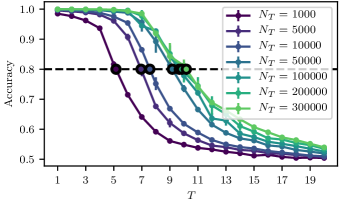
For the results shown in Fig. 7, we keep the network topology fixed and study the performance as a function of prediction time $T$ and the number of training samples. For short times, the accuracy of the network is close to $100\%$, but then it quickly deteriorates as $T$ increases and approaches the random performance of $50\%$. The figure also shows that the performance can be improved with the number of training samples. Increasing their number from $10^{3}$ to $3\cdot 10^{5}$ shows that the time interval over which almost perfect prediction is possible increases, and the point in prediction time where the accuracy decays (defined, e.g., as the point in time where the accuracy falls below $80\%$), increases.

Figure 7: Mean prediction performance. The prediction accuracy is plotted against the prediction horizon $T$ for multiple training datasets. To account for the coverage of the whole chaotic attractor and the stochasticity in the training process, the network is trained three times with different arbitrarily chosen initial seeds and different training sets of size $N_{T}$ based on the same initial seeds. The resulting variance in the performances is shown as error bars. The dashed black line marks $80\%$ accuracy and the circles with black border are drawn at the horizons for which the model performs with $80\%$ accuracy.

Figure 8: Prediction errors. The leading points $(x_{n},y_{n})$ that have been misclassified by the neural network for two prediction horizons, $T=4$ and $T=7$. Blue denotes false positives and red denotes false negatives. The orange and black background is the attractor classified into state space points fulfilling and not fulfilling Eq. (3), respectively, similar to the color coding in Fig. 2.

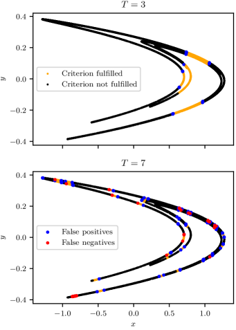
Most of the prediction errors occur at the boundaries of the classes, where two classes meet, see Fig. 8. Hence, the expectation is that increasing $T$ leads to less accurate predictions by increasing the number of intervals and therefore the room for errors by insufficient sampling of the regions and their neighborhood. Consequently, there is a connection between the prediction horizon and the prediction performance through the number of intervals.

To analyze the dependence on the number of samples, we take the fixed performance level of $80\%$, as shown in Fig. 7, and extract the number of time steps for which accuracy is above this value. For instance, for $N_{T}=10^{3}$, this number is $5$, increasing to $7$ with $N_{T}=5\cdot 10^{3}$ and $9$ with $N_{T}=5\cdot 10^{4}$. As Fig. 9 shows, the increase in the number of training samples needed to achieve a certain prediction time increases exponentially, approximately like $40\cdot\exp(1.01T)$.

Figure 9: Relation between the number of training samples $N_{T}$ and the time horizon $T$ up to which the performance is $80\%$ or better. The dashed line shows a fit $N_{T}\propto\exp(sT)$ with $s\approx 1.01$. For larger times the number of training samples increases more steeply as the capacity of the network has been exceeded. Later in the text, performances of networks with higher capacities are demonstrated.

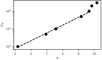
Since the Hénon attractor is chaotic, this increase is expected on account of the positive topological entropy $h$. However, the increase in the number of training samples $s$ is faster than suggested by the topological entropy: with $h=0.465$ and $s=1.01$, it is around twice as large.

For very large numbers of training samples the exponential relation breaks down, see Fig. 9. For example, using $3\cdot 10^{5}$ training samples does not lead to a six-fold prediction performance improvement over $5\cdot 10^{4}$ training samples. The deviation from the exponential relation in Fig. 9 indicates that the performance saturates so that more training samples do not lead to higher accuracy. The origin of this saturation lies in the structure and number of parameters in the network.

To explore the effect of the network, we changed the number of layers and also the number of neurons per layer (compared to the previous baseline topology). As there is no ordering on network topologies, we introduce a class of networks where the number of input layers is fixed (20, for trajectories with 10 steps into the past), the width of the first hidden layer is 32, and this is repeated for a certain number of hidden layers, and then there is an output region of 3 layers, where the number of neurons is (16, 7, 2), with the last one the softmax output used before. This decrease from the full width of 32 to the 2 output neurons is faster than in the case of the network used before, so as to be able to study smaller networks as well. The different networks can then be labeled by $L$, the number of layers with the full width of $32$ neurons, as shown in Fig. 10.

Figure 10: The topologies that are used to check if larger topologies are capable of outperforming smaller ones for larger prediction horizons $T$.

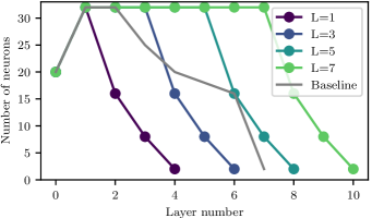
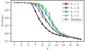
These different network topologies are trained with a fixed number of $10^{5}$ samples. The results are summarized in Fig. 11. Larger topologies shift the plateau to increased prediction horizons $T$. This can be interpreted as larger networks being able to distinguish finer intervals.

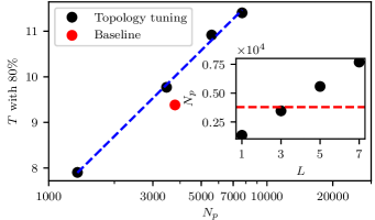
Finally, Fig. 12 shows the relation between the number of parameters $N_{p}$ in the network and the prediction times $T$ at which the different network topologies achieve $80\%$ accuracy. The inset shows the linear increase in the number of parameters $N_{p}$ with the number $L$ of wide hidden layers. As the network has to resolve ever finer regions with increasing time, one anticipates that the number of parameters has to increase, and that the increase should be related to the exponentially increasing number of regions. The data are consistent with a fit $N_{p}\approx 26\exp(0.47T)$, and the exponent $0.47$ is very close to the topological entropy $h=0.465$. Once the parameters of the network are exhausted, it cannot learn new features, and no matter how large the training set, the performance will not improve, which is the origin of the deviation from the exponential behaviour in Fig. 9 for large times.

Having evaluated the requirements for training data size and neural network size to achieve an accuracy of $80\%$ for $N=10$ state space points as input to the neural network, it is studied in preliminary calculations how the variation of $N$ affects these requirements. Due to the high computational costs, the baseline neural network is selected as network topology and trained a single time with $N\in[1,15]$ for different prediction times $T$ and training data sizes $N_{T}$, similar to Fig. 7. For every value of $T$ and $N_{T}$, the performance increases while tuning $N$ from $15$ down to $1$. Hence, all curves in Fig. 7 shift towards the right for smaller values of $N$. The performance increase, however, appears to depend on $N_{T}$: the performance differences between the trainings with different values of $N$ become smaller for more training data $N_{T}$. Consequently, the exponential scaling factor $s$ as computed in Fig. 7 depends on $N$. Nevertheless, they remain positive for all $N$ so that ever more training data is needed to achieve an accuracy of $80\%$.

Figure 11: Accuracy of neural networks of different topologies, trained on $10^{5}$ data samples. The color coding of the topologies corresponds to the one shown in Fig. 8.

Figure 12: Relation between the time horizon $T$ at which the performance is $80\%$ and the number of parameters in the neural network $N_{p}$. The relation follows an exponential behavior in $T$. The inset shows the relation between $N_{p}$ and $L$, the latter as parameter that is used to adjust the number of hidden layers with size $32$. The corresponding properties of the baseline topology are shown in red.

V Conclusions

In the present work, we have analyzed the performance of neural networks for predictions in a chaotic 2d model. The benefit of the 2d map is the ability to visualize the state space of the system and to given a geometric interpretation to the prediction task: the points on the attractor that fall above the prediction threshold are part of geometrically well defined rectangular regions in the state space. As the prediction time increases, so does their number, while their diameter decreases. The network therefore has to classify initial conditions according to whether they fall into these regions or not.

As was to be expected, the performance of sufficiently complex network topologies was very good for a few steps into the future and then deteriorated quickly as the prediction time increased. The prediction errors are localized near the boundaries of the regions, and reflect the fact that a finite number of training samples can only approximate the regions and their boundaries within a certain accuracy. Accordingly, the performance could be improved with an increase in the number of training samples. The number of training samples needed to maintain a certain performance increased more quickly than the number of regions that have to be distinguished.

Increasing the number of training samples increases the performance only up to a point. Eventually, another limitation of the prediction task becomes noticeable, the fact that a finite number of parameters in the network cannot characterize a much larger number of regions, unless they are in some form correlated. Then an improvement in performance can only be achieved by an increase in the number of nodes in the network.

While accuracy and number of training samples are parameters that can easily be ordered as to good and bad or large and small, the network topology remains a variable without natural ordering, and with an irregular influence on the performance. The family of networks with an increasing number of hidden layers of fixed size did show an improved performance with an increase in the number of hidden layers. But it remains to be studied how variations in the width or the shape of the tapering region towards the output region influence the performance. The results in Fig. 11 show that dependence is non-monotonic: the baseline model has a tapering region with five layers, and performance similar to the $L=3$ model with a steep decent towards the output layer. Nevertheless, within a fixed topology, one can find a direct relation between the number of parameters in the network and the number of regions that have to be identified, and both increase exponentially with a rate given by the topological entropy.

In addition to the network topology and the training protocol, also the time history of the trajectory is an important parameter. The results shown here are for a history of $N=10$ steps into the past. First tests for values of $N$ between $1$ and $15$ show that smaller values improve the prediction performances but leaving the main result of exponentially larger training data corpus sizes for longer prediction time horizons in the Hénon map unchanged. The improvement for smaller $N$ are reasonable when taking into account that the Henon map is fully observed and a deterministic chaotic map. However, it should be kept in mind that when $N$ is changed, also the input layer of the network topology changes while the rest of the network remains unchanged in our setup. This results in more network parameters $N_{p}$ per input feature and, hence, an increased network capacity per input feature for smaller numbers of $N$.

The present study is performed for a particular system and for a well-defined numerical task. Nevertheless, the results should also carry over to more general, non-numerical ML tasks, where the number of regions correspond to certain regions in the state space of the system: decisions that depend on regions that are under-resolved or not identified at all by the training sets will naturally be error prone.

The results presented here in conjunction with observations in Pathak et al. (2018) show that Machine Learning ideas provide a set of flexible and easily adapted tools for predicting chaotic dynamical systems, if basic elements of the underlying chaotic dynamics are taken into account, such as the increase in complexity of the task with the prediction time, and the fragmentation of state space by the stretch and fold mechanism. When these conditions are taken into account, ML tools hold great promise for many applications.

One such application in the context of chaotic dynamics is the predicition of relaminarization events in wall-bounded parallel shear flows such as pipe, Couette or channel flow. The transition to turbulence in such flows is subcritical, resulting in the coexistence of an attracting fixed point corresponding to laminar flow and a chaotic saddle representing transient turbulent dynamics. A relaminarization event then corresponds to an escape from the chaotic saddle. A trajectory will therefore never return to the chaotic saddle once it has reached the laminar fixed point, unless it is forced to do so by a finite amplitude perturbation. In the present context this implies that once a relaminarization event has been recorded, a new flow simulation will need to be initialised within the chaotic saddle in order to record the next event. That is, the training process requires a large number of simulations.

The present study confirms the general feasibility of data-driven predictions of extreme events despite chaotic dynamics. However, the input spaces in the fluid dynamics context are of much higher dimension and as such require higher capacities of the neural networks to achieve good prediction results. Additionally, the prediction horizon will have to be chosen with care to ensure sufficiently high performances at non-trivial task difficulty. After all, high neural network performances are required to, eventually, learn previously unknown facts from the neural network.

VI Acknowledgements

We gratefully thank Bruno Eckhardt for his supervision for this project and all the personal and professional advice along our ways, from studies and far beyond. All this will be remembered.

References

- Silver et al. (2017) D. Silver, J. Schrittwieser, K. Simonyan, I. Antonoglou, A. Huang, A. Guez, T. Hubert, L. Baker, M. Lai, A. Bolton, Y. Chen, T. Lillicrap, F. Hui, L. Sifre, G. van den Driessche, T. Graepel, and D. Hassabis, Nature 550, 354 (2017).
- Schuld et al. (2019) M. Schuld, I. Sinayskiy, and F. Petruccione, Physics 12, 74 (2019).
- Jeckel et al. (2019) H. Jeckel, E. Jelli, R. Hartmann, P. K. Singh, R. Mok, J. F. Totz, L. Vidakovic, B. Eckhardt, J. Dunkel, and K. Drescher, Proceedings of the National Academy of Sciences 116, 1489 (2019).
- Carrasquilla and Melko (2017) J. Carrasquilla and R. G. Melko, Nature Physics 13, 431 (2017).
- Butler et al. (2018) K. T. Butler, D. W. Davies, H. Cartwright, O. Isayev, and A. Walsh, Nature 559, 547 (2018).
- Brunton et al. (2019) S. Brunton, B. Noack, and P. Koumoutsakos, arXiv preprint arXiv:1905.11075 (2019).
- Champion et al. (2019) K. Champion, P. Zheng, A. Y. Aravkin, S. L. Brunton, and J. N. Kutz, arXiv (2019), 1906.10612v1 .
- Ott (2002) E. Ott, Chaos in Dynamical Systems, 2nd ed. (Cambridge University Press, 2002).
- Weigend et al. (1990) A. S. Weigend, B. A. Huberman, and D. E. Rumelhart, International Journal of Neural Systems 01, 193 (1990), https://doi.org/10.1142/S0129065790000102 .
- Mukherjee et al. (1997) S. Mukherjee, E. Osuna, and F. Girosi, in Neural Networks for Signal Processing VII. Proceedings of the 1997 IEEE Signal Processing Society Workshop (1997) pp. 511–520.
- Bontempi et al. (2013) G. Bontempi, S. Ben Taieb, and Y.-A. Le Borgne, “Machine learning strategies for time series forecasting,” in Business Intelligence: Second European Summer School, eBISS 2012, Brussels, Belgium, July 15-21, 2012, Tutorial Lectures, edited by M.-A. Aufaure and E. Zimányi (Springer Berlin Heidelberg, Berlin, Heidelberg, 2013) pp. 62–77.
- Pathak et al. (2018) J. Pathak, B. Hunt, M. Girvan, Z. Lu, and E. Ott, Physical review letters 120, 024102 (2018).
- Pathak et al. (2017) J. Pathak, Z. Lu, B. R. Hunt, M. Girvan, and E. Ott, Chaos 27, 121102 (2017).
- Lorenz (1963) E. N. Lorenz, Journal of the atmospheric sciences 20, 130 (1963).
- Hof et al. (2006) B. Hof, J. Westerweel, T. M. Schneider, and B. Eckhardt, Nature 443, 59 (2006).
- Eckhardt et al. (2007) B. Eckhardt, T. M. Schneider, B. Hof, and J. Westerweel, Annu Rev Fluid Mech 39, 447 (2007).
- Eckhardt (2018) B. Eckhardt, Physica A 504, 121 (2018).
- Srinivasan et al. (2019) P. A. Srinivasan, L. Guastoni, H. Azizpour, P. Schlatter, and R. Vinuesa, Phys. Rev. Fluids 4, 054603 (2019).
- Hénon (1976) M. Hénon, Comm. Math. Phys. 50, 69 (1976).
- Artuso et al. (1990) R. Artuso, E. Aurell, and P. Cvitanovic, Nonlinearity 3, 361 (1990).
- Schneider and Eckhardt (2009) T. M. Schneider and B. Eckhardt, Phil Trans R Soc A 367, 577 (2009).
- Goodfellow et al. (2016) I. Goodfellow, Y. Bengio, and A. Courville, Deep learning (MIT press, 2016).
- Heaton (2008) J. Heaton, Introduction to neural networks with Java (Heaton Research, Inc., 2008).
- Kingma and Ba (2014) D. P. Kingma and J. Ba, arXiv preprint arXiv:1412.6980 (2014).
- He and Garcia (2009) H. He and E. A. Garcia, IEEE Transactions on knowledge and data engineering 21, 1263 (2009).