Using Wavelets to Analyze Similarities in Image-Classification Datasets

Abstract.

Deep learning image classifiers usually rely on huge training sets and their training process can be described as learning the similarities and differences among training images. But, images in large training sets are not usually studied from this perspective and fine-level similarities and differences among images is usually overlooked. This is due to lack of fast and efficient computational methods to analyze the contents of these datasets. Some studies aim to identify the influential and redundant training images, but such methods require a model that is already trained on the entire training set. Here, using image processing and numerical analysis tools we develop a practical and fast method to analyze the similarities in image classification datasets. We show that such analysis can provide valuable insights about the datasets and the classification task at hand, prior to training a model. Our method uses wavelet decomposition of images and other numerical analysis tools, with no need for a pre-trained model. Interestingly, the results we obtain corroborate the previous results in the literature that analyzed the similarities using pre-trained CNNs. We show that similar images in standard datasets (such as CIFAR) can be identified in a few seconds, a significant speed-up compared to alternative methods in the literature. By removing the computational speed obstacle, it becomes practical to gain new insights about the contents of datasets and the models trained on them. We show that similarities between training and testing images may provide insights about the generalization of models. Finally, we investigate the similarities between images in relation to decision boundaries of a trained model.

1. Introduction

Studying the similarities and differences among images in training sets may provide valuable insights about the data and the models trained on them. For example, we may identify redundancies and/or anomalies in the training sets, or we may gain insights about the generalization of models on testing sets and understand their misclassifications in relation to training sets. Some studies in the literature aim to identify redundant and influential images in datasets. However, such analysis is performed in a post-hoc way and require a model that is trained on all the data. Here, we leverage image processing and numerical analysis methods for analyzing image classification datasets prior to training. Our computational approach is very fast compared to the methods in the literature. Interestingly, the redundant images that we identify are the same as the results of previous methods that require pre-trained models, confirming the validity of our approach to use wavelets to analyze contents of image classification datasets.

The fast computation makes it practical to provide many useful insights about the contents of image classification datasets. We show that a similarity matrix and analysis of eigen-gaps of a graph Laplacian can provide an estimate about portion of redundancies in the datasets, prior to training a model, which is useful for many applications that rely on automated gathering of vast amount of images with lots of redundancies. Our method can also be used to identify influential images and to create a graphical model representing the contents of image classification datasets.

Moreover, analyzing the similarities across training and testing sets may provide insights about the generalization in deep learning.

Figure 1. Example of nearly identical images in CIFAR-10 training set.

Figure 2. Example of similar images with different labels in CIFAR-100 training set: oak and maple tree (left), whale and seal (right).

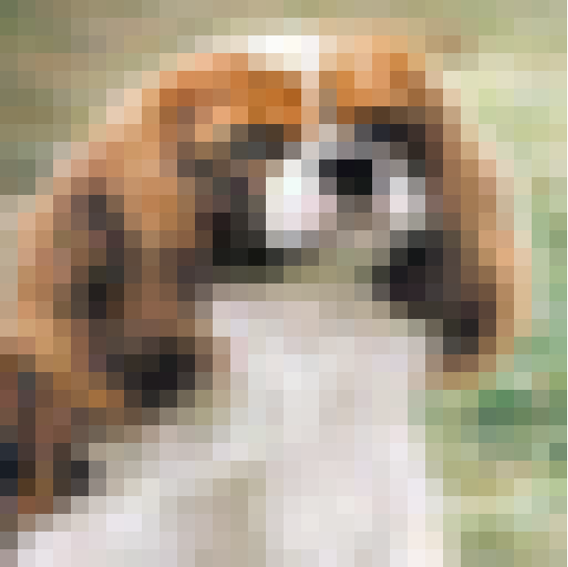
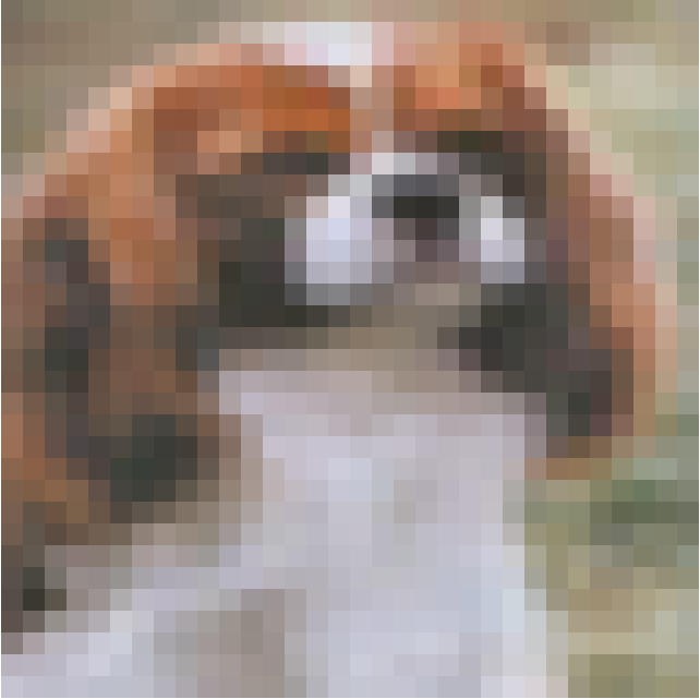
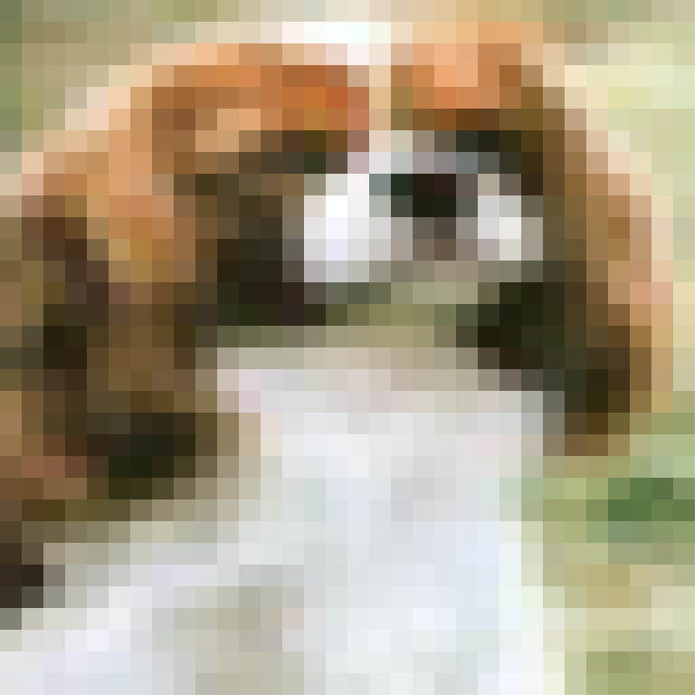
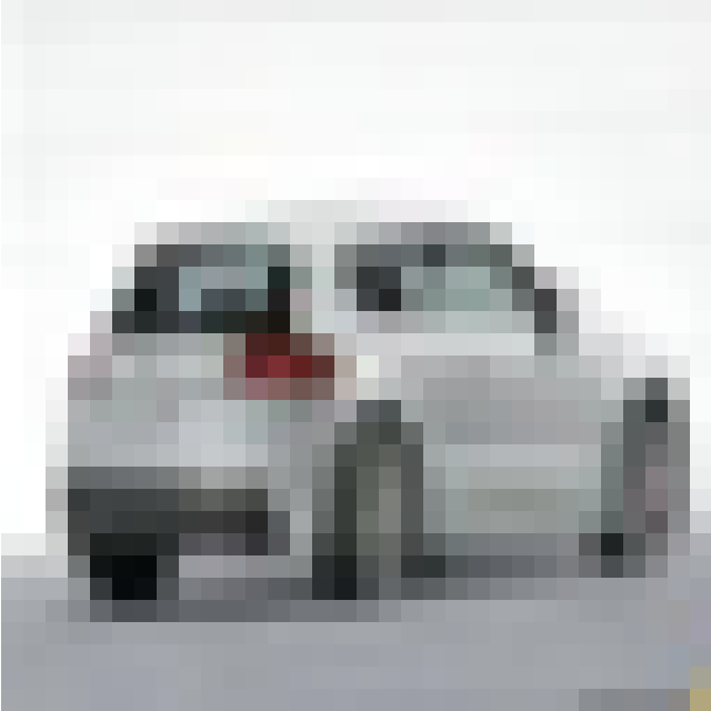
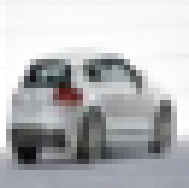
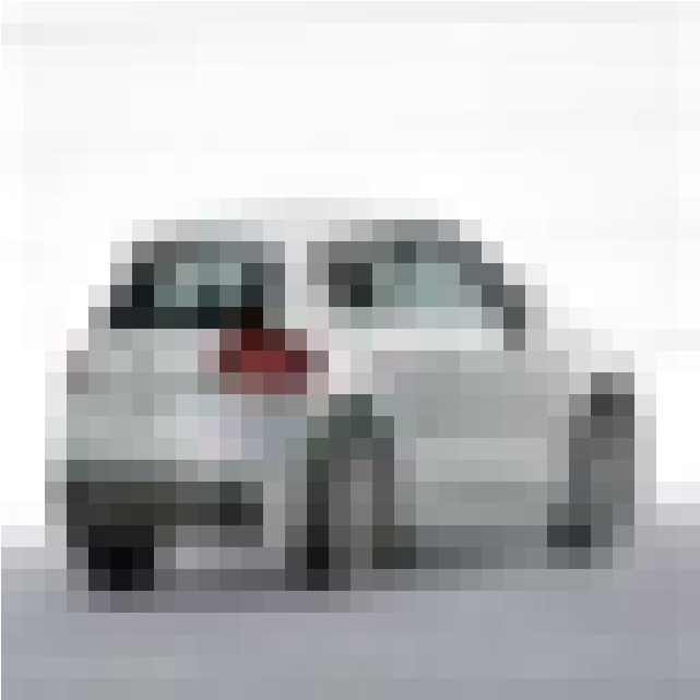
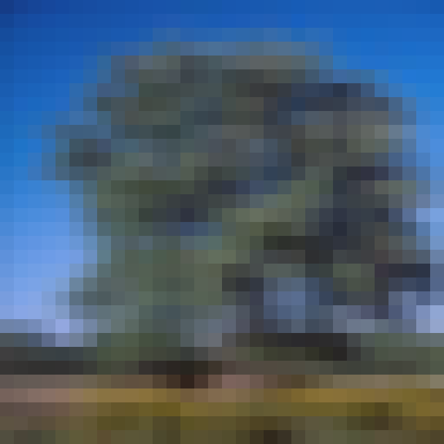
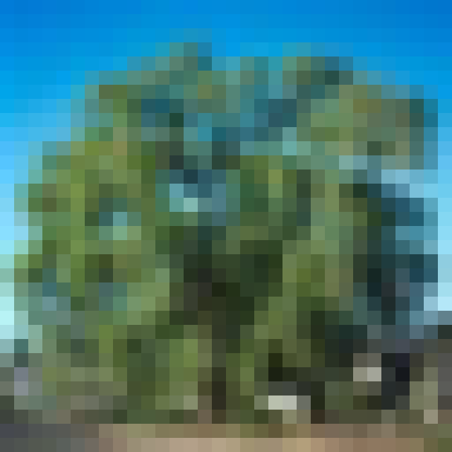
Figure 1 shows examples of redundancies present in the CIFAR-10 dataset and Figure 2 shows examples of similar images with different labels in the CIFAR-100 dataset. Our method identifes all of such similarities in a few seconds, with no need for a trained model.

1.1. Image classifiers and their decision boundaries

Any classification model is defined by its decision boundaries, and hence, training process of a model can be viewed as defining those decision boundaries for the model. Consider for example, the case of training a linear regression model. What happens during the training is basically defining the location of the regression line (i.e., decision boundary) to partition the input space. Training of an image classification model is also partitioning its input space, although such partitions can be geometrically complex in the high dimensional space.

From this perspective, any training image that does not affect the decision boundaries of a model can be considered redundant, and any training image that affects the partitioning of the input space can be considered influential. Therefore, when a group of images from the same class are similar, it is likely that only one of them would suffice to define the necessary decision boundary in that neighborhood in the domain.

On the other hand, when images of different class are similar (e.g., see Figure 2), they would be influential, because they are similar, and learning them would cause the model to define the necessary decision boundaries between them. We study these conjectures in our numerical experiments.

1.2. Our plan

We propose one general approach and two specific implementations to analyze the similarities in image-classification datasets. The general approach is to use wavelets to measure the similarities among images and to analyze those similarities to provide insights about the contents of datasets.

Our first implementation (Algorithm 1) is fast and effective as it decomposes images and clusters them based on their similarities. Any clustering method can be used. Our second implementation (Algorithm 2) performs a more thorough analysis of datasets by forming a similarity matrix and investigating the eigen-gaps of a graph Laplacian. We later show that this can provide a graphical model and reveal possible anomalies in the dataset.

We show the effectiveness of our methods on standard object recognition datasets such as CIFAR-10 and CIFAR-100 (Krizhevsky et al., 2009), and also one class of Google Landmarks dataset (Noh et al., 2017).

In Section 2, we review the related work. In Sections 3 and 4, we describe each of our methods, respectively. Section 6 includes our numerical results, and finally, in Section 7, we discuss our conclusions and directions for future research.

2. Related work

One of the early studies in the literature is by Ohno-Machado et al. (1998) which reports existence of redundancies in medical training sets, but their computational method is not practical for modern applications of deep learning.

There are studies that measure the influence of training points based on the derivatives of the loss function of a trained model. Guo and Schuurmans (2008) studied the derivatives of mini-batches to select subsets of unlabeled data but their method is specific to active learning, where there is a stream of new training data. Vodrahalli et al. (2018) showed that choosing training images with most diversity of derivatives can speed up the training, but their analysis is based on models trained on all the data. Recently, (Sankararaman et al., 2019) explained the speed of training in terms of correlation between gradients.

There are also methods that consider the value of loss function or norm of gradients (Loshchilov and Hutter, 2015; Alain et al., 2015; Katharopoulos and Fleuret, 2018). Such measures are useful to speed up the training, but not necessarily meaningful proxies to compare similarity of images. Additionally, since they require computation of loss and gradient of a model, they are more expensive than direct comparison of images using image processing tools.

Lapedriza et al. (2013) proposed a greedy method to sort the data points in training sets based on their importance for training. For the sorting, they define a “training value” which requires the model to be separately trained from scratch for each training image.

Influence functions have been used to quantify the effect of individual training data on a trained model (Koh and Liang, 2017; Koh et al., 2019), but the assessment of influence requires a model trained on all the data.

Carlini et al. (2018) developed a method that first projects the images from the pixel space into a two dimensional space, and then performs clustering in the low dimensional space, but the projection requires a model trained on all the training set.

There are other studies focused on interpretability of image classification models that make use of prototypes, for example, (Kim et al., 2014; Li et al., 2018; Chen et al., 2019). Such methods aim to train a model such that its output is explainable in terms of similarity to prototypes. To compare an image with a prototype, Chen et al. (2019) inverts the $\ell_{2}$ norm distance between the output of a trained convolutional layer and the prototype.

Meletis et al. (2019) used a Gaussian Mixture Model (GMM) to identify visually similar images using a pre-trained model.

Birodkar et al. (2019) used clustering of images in a semantic space to identify redundant images. The semantic space in their study is the intermediate output of a trained model. Barz and Denzler (2019) also showed that redundant images in CIFAR datasets can be identified using the output of an average pooling layer.

Chitta et al. (2019) showed that a portion of some training sets can be removed leading to no loss of accuracy. Their method trains an ensemble of deep neural networks on all the training set in order to identify such redundancies. Yousefzadeh and O’Leary (2020) showed that the distance of training images to the decision boundaries of a trained model can identify the most influential training data.

All the approaches above identify the influence of training images through the lens of a model that is trained on all the data. Here, we show that using wavelets, one can analyze the images and obtain valuable information about them, before engaging in the training process.

Achille et al. (2019) studied the similarities between different image classification tasks, e.g., classifying different kinds of birds vs different kinds of mammals, which can provide valuable information about the nature of those classification tasks, however, their approach requires model training.

Finally, we note that there are unsupervised methods that aim to create an embedding for groups of images. For example, (Vo et al., 2019) solves an optimization problem for each image pair to measure their similarity and then creates an embedding based on that information. However, such methods are not scalable to analyze an entire training set.

3. Finding similar (redundant and influential) images in the data

Here, we develop a simple and fast algorithm to identify similar images in training sets. Our algorithm first decompose the images using wavelets, then chooses a subset of wavelet coefficients that have the most variation among images. Finally, it clusters the images based on their wavelet coefficients. Images that are similar will appear in same clusters and that lead to identifying influential and redundant images. Repeating the same analysis on testing sets can also provide insights about testing sets.

3.1. Wavelet decomposition of images

We use the wavelet transformation of images as a mean to identify similar training data. Wavelets are a class of functions that have shown to be very effective in analyzing different kinds of data, especially images and signals. Wavelets can also be used to analyze functions and operators (Daubechies, 1992). In both image processing and signal processing, wavelets have been effective in compressing the data and also in identifying actual data from the noise (Chui, 2016).

The main idea here is to decompose each image into different frequency components and then analyze the components among the images to identify their similarities and differences. Wavelets allow us to analyze images at different resolutions and therefore enable us to compare them effectively.

Decomposing an image using a wavelet basis is basically convolving the wavelet basis over the image. This is similar to the operation performed by convolutional neural networks, as CNNs also convolve a stencil with the input image. Therefore, our method of analyzing and comparing images is similar to the computational method that will be used by the classification models. In our results, we see that wavelets identify the similarity of images, in the same way that a pre-trained ResNet-50 does.

In this paper we use wavelets, but we note that shearlets (Kutyniok and Labate, 2012) are also a class of functions with great success in analyzing images, and therefore they can be considered instead of wavelets.

3.2. Extracting a subset of influential wavelet coefficients

We are interested in the similarities and differences among subgroups of images. But, as we will show in our numerical experiments, many of the wavelet coefficients can be similar among all images in a training set and therefore, not helpful for our analysis.

When computing wavelet decomposition, one can use different resolutions to convolve the wavelet basis with images. Since we are concerned with the overall similarity of images, there will be no need to extract the wavelet coefficients on a very fine level. Therefore, even for relatively large images in Imagenet and Google Landmarks datasets, one can extract a relatively small number of wavelet coefficients by convolving the images with high pass filters.

Once we have computed the wavelet coefficients for images, we use rank-revealing QR factorization (Chan, 1987) to choose a subset of coefficients that are most linearly independent among the images. Rank-revealing QR algorithm and also its variation, pivoted QR algorithm (Golub and Van Loan, 2012) decompose a matrix by computing a column permutation and a QR factorization of a given matrix. The permutation matrix orders the columns of the matrix such that the most linearly independent (non-redundant) columns are moved to the left. The rows of our matrix represent the images and its columns represent wavelet coefficients.

The obtained permutation matrix allows us to choose a subset of most independent columns. This dimensionality reduction in the wavelet space, previously used by Yousefzadeh and O’Leary (2019a, b), can make our next computational step (i.e., clustering) faster.

As an example, consider the 60,000 images in the training set of MNIST dataset. Each image has 784 pixels, leading to 784 wavelet coefficients using the Haar wavelet basis. 32 of those wavelet coefficients are 0 for all images. After discarding those coefficients, the condition number of the training set is greater than $10^{22}$, implying linear dependency of columns. After performing rank-revealing QR factorization, we observe that dropping the last 200 columns in the permutation matrix will decrease the condition number to about $10^{6}$. All the discarded features will be completely unhelpful in identifying influential and redundant data, because they are either uniform or (almost) linearly dependent among all images.

The cost of computing the rank-revealing QR factorization is $\mathcal{O}(nd^{2})$ given $n$ images with $d$ wavelet coefficients (Golub and Van Loan, 2012). We would not need to compute the entire decomposition as the computation can be stopped as soon as a diagonal element of $R$ becomes small enough compared to its first diagonal element.

We note that the possible computational advantage of using rank-revealing QR depends on the relative values of $n$, $d$, and also the computational cost of clustering method which will be discussed in the following.

3.3. Clustering images based on their wavelet coefficients

Any clustering method can be utilized to cluster the images based on their wavelet coefficients. The computational effort for clustering depends on the number of observations (size of training set) and also the number of features considered for each image. We suggest performing the clustering on the entire dataset (when possible), noting that it will be a more expensive computation compared to clustering images of each class, separately. Clustering per class would cost less, but would not provide the additional insight about influential images.

The usual trade-offs among the clustering methods apply here as well. Some clustering methods identify the appropriate number of clusters in the data during the clustering, for example Newman’s community structure algorithms (Newman, 2004), which would be useful when we are not aware of the percentage of similarities in the dataset. But, when the number of clusters is known beforehand, a less costly clustering method could suffice, for example k-means (Lloyd, 1982; Arthur and Vassilvitskii, 2007).

3.4. Our algorithm based on wavelet coefficients and clustering

Algorithm 1 Algorithm for finding similar training images using wavelet coefficients and clustering

Inputs: Training set $\mathcal{D}^{tr}$, $\tau$, clustering method $\mathcal{M}$, $n_{c}$
Outputs: Reduced training set $\mathcal{\hat{D}}^{tr}$ and the list of most influential images $\mathcal{I}$

1:  Count number of images in $\mathcal{D}^{tr}$ as $n$

2:  for $i=1$ to $n$ do

3:     Compute wavelet coefficients of image $i$, vectorize them and save them in row $i$ of matrix $W$

4:  end for

5:  if $n>$ number of wavelet coefficients per image then

6:     $[Q,R,P]=\text{RR-QR}(W)$, i.e. perform rank-revealing QR on $W$

7:     Choose $m$ as large as possible such that the first $m$ columns of the matrix $WP$ has condition number less than $\tau$

8:     Extract the first $m$ columns of $WP$ and save it as $\hat{W}$

9:  end if

10:  Perform clustering on $\hat{W}$ using method $\mathcal{M}$ (with $n_{c}$ clusters)

11:  for $i=1$ to $n_{c}$ do

12:     if there are more than one image in cluster $i$ then

13:        if all images in the cluster are from the same class then

14:           Keep the image closest to the center of that cluster and discard other images

15:        else

16:           Add the images in the cluster to the list $\mathcal{I}$

17:        end if

18:     end if

19:  end for

20:  Put together remaining images in clusters as $\mathcal{\hat{D}}^{tr}$

21:  return $\mathcal{\hat{D}}^{tr}$ and $\mathcal{I}$

Algorithm 1 formalizes the above process in detail. The algorithm first computes wavelet decomposition of all images in the training set and forms them in a matrix $W$, where rows are samples and columns are wavelet coefficients (lines 1 through 4). The next step in the algorithm is to compute the rank-revealing QR factorization of $W$ (line 5). This factorization computes an orthogonal matrix $Q$, an upper-triangular matrix $R$, and a permutation matrix $P$, such that

$${W}{P}={Q}{R}.$$

Algorithm 1 then chooses a subset of $m$ most independent wavelet coefficients according to the permutation matrix (lines 6 and 7). The condition for choosing $m$ is to maximize its value such that the condition number of the first $m$ columns of $WP$ is less than $\tau$. For a given dataset, this condition will yield a unique value for $m$. The best value for $\tau$ could vary based on the properties of the dataset. The trade-off here is that choosing a small $\tau$ will yield a small $m$, making the clustering computation less expensive, while using a very small $m$ may not be able to adequately capture the variations among images and lead to poor results. In our numerical experiments, we found $\tau=10^{5}$ to be a good choice. The final stage of the algorithm is to perform clustering, discard the redundant images, and return the list of influential images (lines 9 through 13).

About the number of clusters, $n_{c}$, its best value would depend on the portion of similar images in a training set which is likely to be unknown. In typical image classification datasets, the portion of similar images (including both same and differing classes) make up less than half of datasets. So, the clustering step can be considered coarse-graining. There are many methods available to choose an appropriate value for $n_{c}$. Later, we describe and use a method that chooses the $n_{c}$ based on the eigen-gaps of graph Laplacian derived from a similarity matrix.

4. Comparing images using specialized image processing tools and analyzing a similarity matrix

Algorithm 1 computes the wavelet decomposition of images and compares the images based on the similarity of their wavelet coefficients in the Euclidean space. We show in our results that this is adequate for analyzing the similarity of images in standard datasets for object recognition. However, we note that there are more sophisticated methods to compare images which we consider in this section.

4.1. Specialized wavelet-based similarity measures between images

There are many methods in the image processing literature for measuring the similarities between images, for example, (Reisenhofer et al., 2018; Wang and Simoncelli, 2005; Sampat et al., 2009). Albanesi et al. (2018) recently proposed a class of metrics to measure the similarity between pairs of images. Here, we use a relatively recent and widely used method known as the Structural Similarity Index (SSIM), developed by Wang et al. (2004), which compares images based on local patterns of pixel intensities that have been normalized for luminance and contrast.

Some of these measures are designed to measure specific kinds of similarity, for example, structural similarity, perceptual similarity, textural similarity, etc. Considering the structure of images and patterns of pixel intensities make the SSIM particularly useful for image classification of objects such as the ones in CIFAR and Imagenet datasets.

We note that the similarity measure should be chosen based on the classification task at hand. For example, in classifying images of skin cancer (Tschandl et al., 2018), the textures present in images may be more influential in classifications, instead of the structure of images. In such case, a texture-based similarity measure such as (Zujovic et al., 2013) may be more effective than the SSIM.

Additionally, many of these measures are tunable. For example, SSIM measures the similarity of images based on three components: luminance, contrast, and structure, and returns an overall similarity score based on them. The weight of components and other tunable parameters of SSIM can be adjusted to measure the specific similarities of interest.

We note that in the image processing literature, image retrieval techniques aim to find images in a dataset that are similar to a base image, some of which use wavelets, for example (Loupias et al., 2000). Our use of wavelet decomposition of images (instead of their pixels) is similar in nature to some of those image retrieval techniques. However, those techniques are not directly applicable for our purpose of analyzing image-classification datasets from the perspective of deep learning. One contribution of our work is to bridge one of the gaps between image processing and deep learning literatures.

4.2. Our algorithm for similarity matrix analysis

Here, we develop Algorithm 2 to perform the analysis via a similarity matrix.

For each image pair in a training set, we compute their similarity using a function of choice $\mathcal{F}$, and form a similarity matrix, $\mathcal{S}$ (lines 3 through 7 in Algorithm 2).

As mentioned in previous section, $\mathcal{F}$ should be chosen based on the patterns present in images and the type of similarities and differences among them. In some datasets, we observed that even the cosine similarity between vectors of wavelet coefficients can be insightful.

After computing the $\mathcal{S}$, our algorithm computes the eigenvalues of its graph Laplacian (line 8). Laplacian is the matrix representation of a graph corresponding to the similarity matrix. Instead of computing the precise eigenvalues, one can compute an estimate to the distribution of eigenvalues, using a Lanczos-based method, e.g., the method developed by Dong et al. (2019). The next step is to choose the number of clusters, $n_{c}$, based on the number of eigen-gaps of the graph Laplacian, as suggested by von Luxburg (2007) (line 9). These two lines of the algorithm can be skipped, if the user wants to use a specific $n_{c}$, for example based on prior knowledge about the dataset.

The algorithm then completes the spectral clustering. The process of discarding redundant training data is similar to Algorithm 1. Overall, this approach has $\mathcal{O}(n^{3})$ because of the spectral clustering.

Algorithm 2 Algorithm for analyzing training images using a similarity matrix

Inputs: Training set $\mathcal{D}^{tr}$, threshold on eigen-gaps $\gamma$, similarity function $\mathcal{F}$
Outputs: Reduced training set $\mathcal{\hat{D}}^{tr}$ and the list of most influential images $\mathcal{I}$

1:  Count number of images in $\mathcal{D}^{tr}$ as $n$

2:  Initialize similarity matrix $S_{n\times n}$ as matrix of zeros

3:  for $i=1$ to $n-1$ do

4:     for $j=i+1$ to $n$ do

5:        $S_{i,j}=S_{j,i}=\mathcal{F}(\text{image }$i$,\text{image }$j$)$

6:     end for

7:  end for

8:  Compute the eigenvalues of the graph Laplacian of $\mathcal{S}$, or an estimate to the distribution of eigenvalues.

9:  Count the eigen-gaps larger than $\gamma$ and use it as $n_{c}$

10:  Complete the spectral clustering on $\mathcal{S}$ with $n_{c}$

11:  for $i=1$ to $n_{c}$ do

12:     if there are more than one image in cluster $i$ then

13:        if all images in the cluster are from the same class then

14:           Keep the image closest to the center of that cluster and discard other images

15:        else

16:           Add the images in the cluster to the list $\mathcal{I}$

17:        end if

18:     end if

19:  end for

20:  Put together remaining images in clusters as $\mathcal{\hat{D}}^{tr}$

21:  return $\mathcal{\hat{D}}^{tr}$ and $\mathcal{I}$

A low-cost alternative to spectral clustering is to check for each image, whether there are any other images similar to it and keep only one image from each group of images that have SSIM larger than a threshold. This basically requires investigating individual rows in the upper triangular section of $\mathcal{S}$. The complexity of such algorithm is $\mathcal{O}(n^{2})$ which might be appealing for large training sets.

We note that SSIM can be used in conjunction with other clustering methods, for example, k-means, leading to $\mathcal{O}(n)$ cost. In such approach, larger similarity between an image pair will be interpreted as closer distance between them and vice versa.

For datasets with large images, it is possible to compress the images first and then perform the analysis. The effectiveness of such approach would depend on the contents of images in the dataset.

5. Insights about generalization of image classifiers

Generalization of image classification models is an open research problem. Deep learning has been impressively successful in image classification, but the reason behind the accuracy of models and also their mistakes is not well understood. Zhang et al. (2016) famously showed that many traditional approaches (model properties or regularization techniques) fail to explain the generalization in deep learning and hence initiated a series of fundamental studies about generalization. Some recent studies relate the generalization to decision boundaries of models, for example (Jiang et al., 2019; Elsayed et al., 2018). Huang et al. (2019) used a visualization method to provide insights about generalization. Kernel methods (Belkin et al., 2018) and compression methods (Arora et al., 2018; Li et al., 2020) are used to study generalization, too. From the optimization perspective, Arora et al. (2019) studied the generalization of models by studying the details of training process. All of these approaches study the trained models and/or training process, and usually overlook the fine-level similarities in the training and testing sets.

Here, we show that analyzing the similarities between training and testing sets may provide additional insights. We observe that for standard datasets like CIFAR-10 and CIFAR-100, a portion of testing sets have nearly identical samples in the training sets. We also observe that mistakes of some classification models are testing images that are either not similar to any image in the training set, or they are similar to training images with different label.

On the other hand, for the state of the art models that achieve nearly perfect accuracies (e.g., 99.4% on CIFAR-10), we observe that their few testing mistakes does not seem to be explainable by similarity of images. In fact we see that some of those testing mistakes have nearly identical training samples. We know that image classifiers are highly over-parameterized and there are infinite minimizers for training loss. The art of achieving high accuracy is in fact finding the minimizer of training loss that achieves good accuracy on the testing set. But, can we choose the best minimizer of training loss without looking at the testing set? If one did not have access to testing set of CIFAR-10 dataset, could they pick the model that achieves nearly perfect accuracy on testing set by just learning the training set?

This type of analysis makes it possible to gain insights about the generalization of models for individual images in terms of their similarities with training sets. It also makes it possible to have some measure of confidence about the accuracy of classifications for unlabeled images. For example, if a testing image is nearly identical to some training images of one class, and not similar to training images of any other class, we can be more confident in the accuracy of model’s classification. But, if a testing image is dissimilar to all the training set, or it is similar to several images from different classes, we can be less confident in the accuracy of classification for that image.

Moreover, in active learning, an analysis of training set may guide us to acquire images that are less abundant in training set.

6. Numerical experiments

Here, we investigate the similarities in three datasets: CIFAR-10, CIFAR-100, and one class of Google Landmarks dataset. The code implementing our methods will be available online.

6.1. CIFAR-10 dataset

We use the 2D Daubechies wavelets to decompose all images in this dataset. The matrix of wavelet coefficients has 50,000 rows and 3,072 columns and its condition number is 21,618. We use all the wavelet coefficients, because the condition number of matrix is not very large.

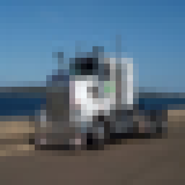
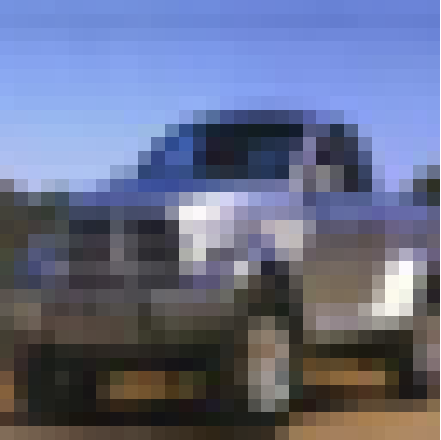
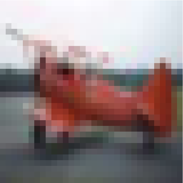
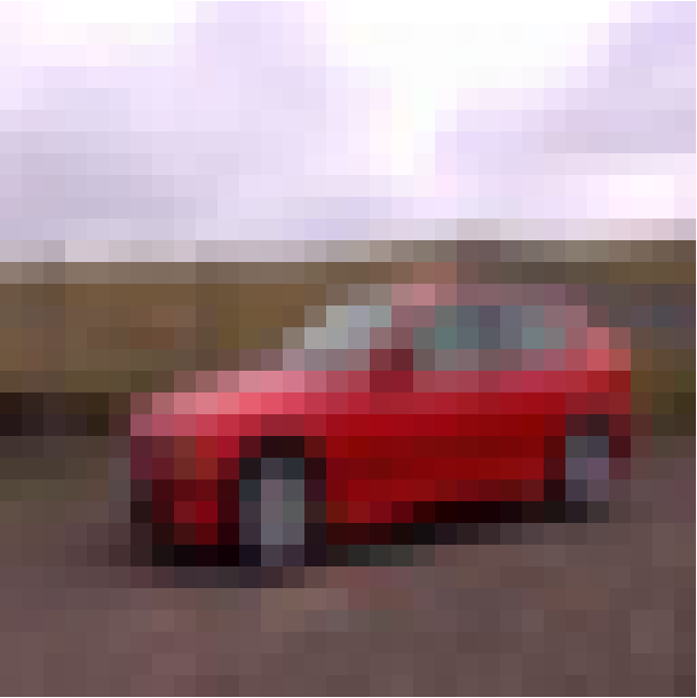
Using Algorithm 1, we cluster the images. We later explain a method for choosing $n_{c}$ based on an eigen value analysis. But, here we choose $n_{c}=47,000$ based on the percentage of redundancies reported by (Birodkar et al., 2019). Figure 3 shows images in some of the clusters with uniform label. Interestingly, the similar images we obtain are the same as the similar images reported by (Birodkar et al., 2019, Appendix). They showed that training a model without the redundant images does not adversely affect the accuracy of models on the testing set. Since our results corroborate their results, there is no need to repeat their experiments on the testing accuracy. One training image per each of these clusters can suffice for training.

The method used by (Birodkar et al., 2019), however, requires training a ResNet model on the entire dataset, a process which can take a few GPU hours for the CIFAR-10 dataset. Our contribution here is our fast computational method that identifies similar images very fast. Our other contribution is to report that wavelets identify the similarity of images, in the same way that a pre-trained ResNet-50 does.

Figure 3. Example of similar images of same class in CIFAR-10 training set. Images in each box have formed one of the clusters. We see that a standard ResNet model does not have any decision boundaries between images of each group, while it has decision boundaries between dissimilar images of same class.

Our fast algorithm makes the analysis of contents of image classification models practical, and therefore opens the door to provide additional insights about large datasets, beyond identifying redundancies.

Figure 4 shows some of the same cluster images that have different labels. Clearly, it is desirable for a model to learn these images and be able to distinguish them from each other.

Figure 4. Some of the similar images with different labels in CIFAR-10 training set. Each box shows one cluster. We consider these images influential in learning.

6.2. CIFAR-100 dataset

We identify redundancies in the CIFAR-100 training set, too, as briefly shown in Figure 5.

Figure 5. Example of redundant images in CIFAR-100 training set.

Similar images with different labels are abundant in this dataset and might be even hard to distinguish for a human. For example, the image pair in the left box in Figure 2 represent a maple tree and an oak tree, and the image pair in the right box represent a whale and a seal.

6.2.1. Class of aquarium fish (training set)

To gain more insight and to compare our algorithms, here, we consider only the second class of this dataset with 5,000 images.

Starting by Algorithm 1, the matrix of wavelet coefficients for this class is $5,000\times 3,072$, with condition number $4\times 10^{18}$. Numerical rank of this matrix is 495, using rank tolerance of $\tau=10^{-5}$. We identify the 495 wavelet coefficients using rank-revealing QR factorization and use them for clustering with $n_{c}=470$. The entire computation takes about 5 seconds on a machine with a 2.30GHz CPU and 115GB of RAM. We obtain redundant images as shown in Figure 6.

Figure 6. Example of redundant images in the aquarium fish class of CIFAR-100.

Let’s see how Algorithm 2 performs and what additional information it can provide. According to the SSIM measure, there are 5 pairs of identical images, all of which are also picked by Algorithm 1 (shown in Figure 6). In contrast, Figure 7 shows two of the most dissimilar image pairs based on the SSIM measure.

Figure 7. Two most dissimilar image pairs in the aquarium fish class of CIFAR-100, based on the SSIM measure. SSIM is -0.5420 for images in the left box and -0.5025 for the right box.

The mean value of the similarity matrix, $\mathcal{S}$, is 0.088 and its standard deviation is 0.131. Figure 8 shows the distribution of eigenvalues of its graph Laplacian, implying that there are not any large clusters in the data. We choose the number of clusters based on the eigen-gaps of the graph Laplacian. Using the eigen-gap threshhold as 0.4 leads to $n_{c}=454$.

Figure 8. Distribution of eigenvalues of the graph Laplacian for all images in the “aquarium fish” class of CIFAR-100.

Spectral clustering then yields clusters with all the identical pairs mentioned above, with some additional images that are fairly similar, as two pairs are shown in Figure 9 because we chose a smaller $n_{c}$.

Figure 9. Examples of similar training images in CIFAR-100.

In summary, the results of our two algorithms corroborate each other. Algorithm 2 is more expensive for this example as expected, however, it provides more detailed insights about the images and guides us to choose a wise value for the number of clusters.

6.3. Generalization of models

6.3.1. Class of aquarium fish of CIFAR-100 (training and testing sets)

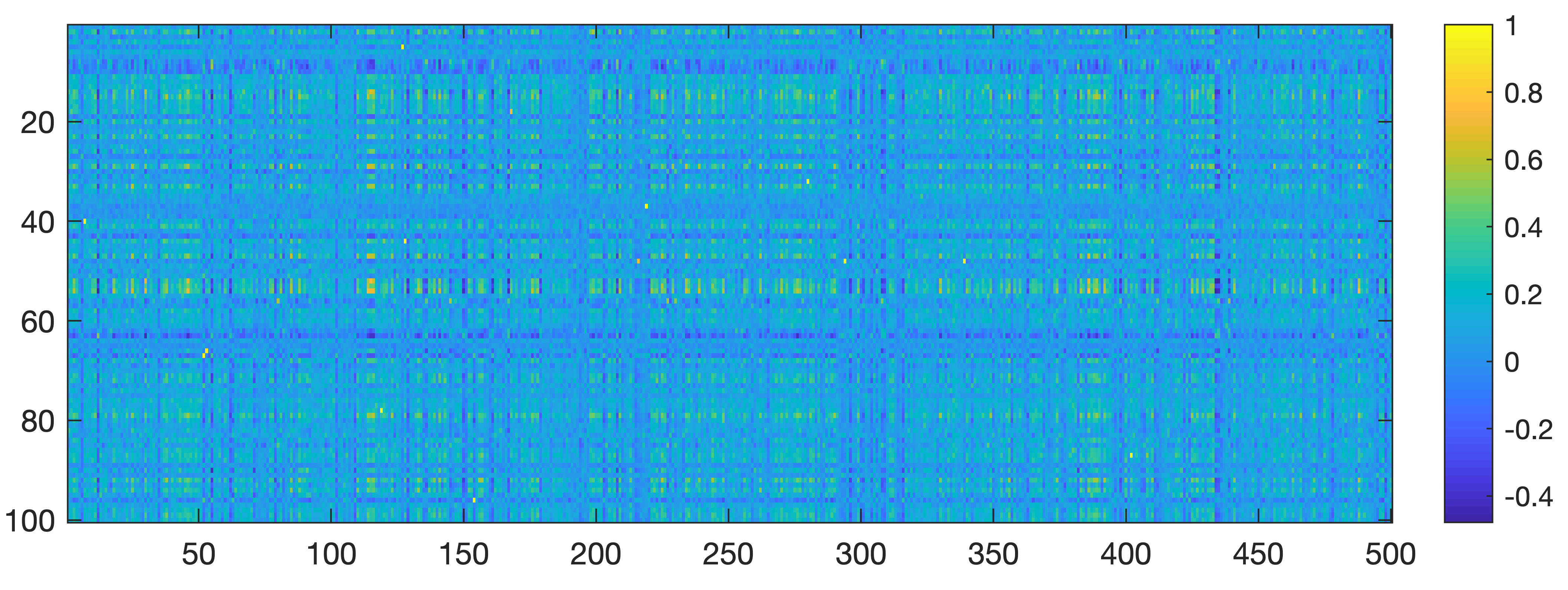
We compare all 100 testing images of this class to all 500 training images of this class. The similarity matrix is shown in Figure 10. This analysis shows that 11% of testing images have a nearly identical image in training set. Figure 11 shows three testing images that have the least similarity to all images in the training set which are among the mistakes of some classification models on CIFAR-100.

Figure 10. The similarity matrix between 100 testing images and 500 training images of the aquarium fish class in CIFAR-100.

Figure 11. Testing images most dissimilar from the training set for the aquarium fish class. These happen to be common mistakes of some models.

6.3.2. Classes of cat and dog of CIFAR-10 (training and testing sets)

We consider the model developed by Kolesnikov et al. (2019) which has reported the best accuracy on CIFAR-10. This model only makes 65 misclassifications out of the entire 10,000 testing images of CIFAR-10 dataset. 19 of those mistakes are either misclassifying a dog as a cat, or the reverse. So, we consider those two classes and analyze the similarities between their training and testing images.

In this case, we decompose images using the Daubechies 2 wavelets, measure their distance in Euclidean space, and then convert the distance to a similarity measure using Gaussian kernels.

Testing images of Cat that are misclassified as Dog by (Kolesnikov et al., 2019) are shown in Figure 12. Consider the image at the bottom right in this Figure. The three most similar training images to it (from both Cat and Dog classes) are shown in Figure 13, all of which have cat label and are considerably similar to the misclassified testing image. So, absence of similar training data with same label, nor presence of similar training data with opposite label may not be the cause of misclassification.

Figure 12. Testing images of cat in CIFAR-10 that are misclassified by the state of art model.

Figure 13. (left) A testing image misclassified by the state of art model on CIFAR-10. (right) Three training images most similar to the image on left, all labeled as cat.

On the other hand, there are correctly classified testing images that can be considered isolated from the training set. Figure 14 shows the three testing images of Cat class that are most dissimilar to the entire training set of cats and dogs. The model developed by (Kolesnikov et al., 2019) correctly classifies them as cat.

Figure 14. Testing images most dissimilar from the training set for the cat class of CIFAR-10.

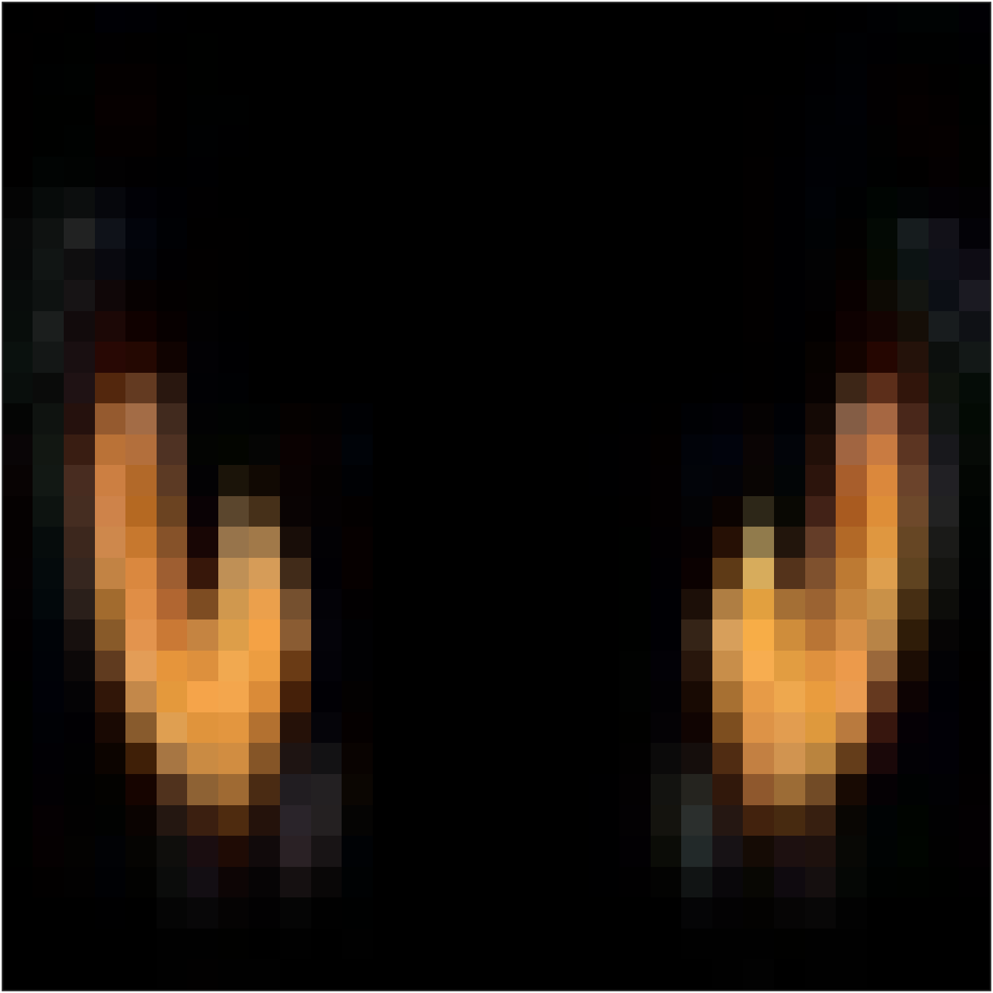
Moreover, there are testing images of cat that are more similar to training images of dogs compared to training images of cats. Figure 15 shows three of those, all of which are correctly classified as cat by (Kolesnikov et al., 2019).

Figure 15. Testing images of cat in CIFAR-10 that are more similar to training images of dogs, compared to training images of cats.

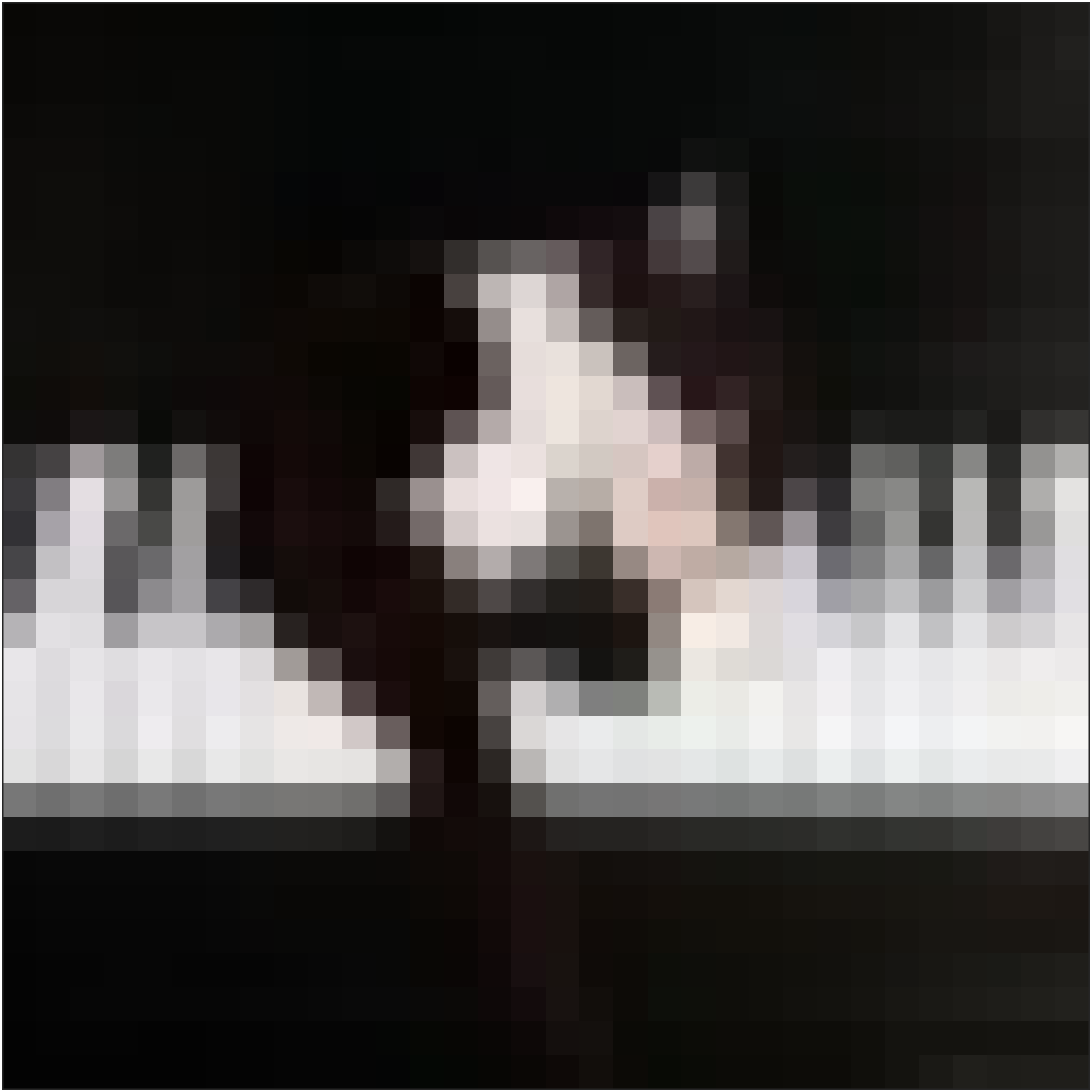
It is becoming common in the literature to conduct surveys about the mistakes of the models and ask humans whether they can classify them correctly, in order to justify the mistakes. However to our knowledge, surveys are not conducted about correctly classified testing images. In fact one might wonder why the image in the middle of Figure 14 and the rightmost image in Figure 15 are labeled as cat.

We hope that these observations lead to meaningful questions and answers about the generalization in deep learning.

6.4. Influence of training data on decision boundaries of a trained model

We consider the standard ResNet-v2 models (He et al., 2016), pre-trained on CIFAR-10 and CIFAR-100 datasets and investigate their decision boundaries in relation to these images. A model’s decision boundary between two class is any point that produces equal softmax scores for those, while the softmax score for all other classes are less than those (Elsayed et al., 2018; Yousefzadeh and O’Leary, 2020).

We aim to find whether the output of the model along the direct path connecting two images hits a decision boundary or not. In other words, we want to find out whether the model has a decision boundary defined between two images. The direct path between two images $\bf{x_{1}}$ and $\bf{x_{2}}$ is defined by $(1-\alpha)\bf{x_{1}}+\alpha\bf{x_{2}}$, where $\alpha$ is a scalar between 0 and 1.

As expected, images that are almost identical in Figures 1,5, and 6, do not have any decision boundary between them. On the other hand, images of the same class that are not similar do have decision boundaries between them, for example, images in Figure 7. This means that the model output along the direct path between such images exits the correct classification and re-enters it, hitting at least two decision boundaries in between. Interestingly, groups of images in Figures 3 and 9 that are similar but not identical, do not have any decision boundaries between them. This can be the subject of further study.

6.5. Google Landmarks dataset v2

For this dataset, we consider the class of Verrazzano-Narrows bridge. There are 56 images for this class which we standardized as 512 by 662 pixels. Using Algorithm 2, we analyze all training images in this class. Figure 16 shows the similarity matrix of images in the class and Figure 17 shows a graphical model derived from the similarity matrix.

Figure 16. The similarity matrix for the class of Verrazzano-Narrows bridge in the Google Landmarks dataset v2.

Figure 17. The graphical model derived from the similarity matrix.

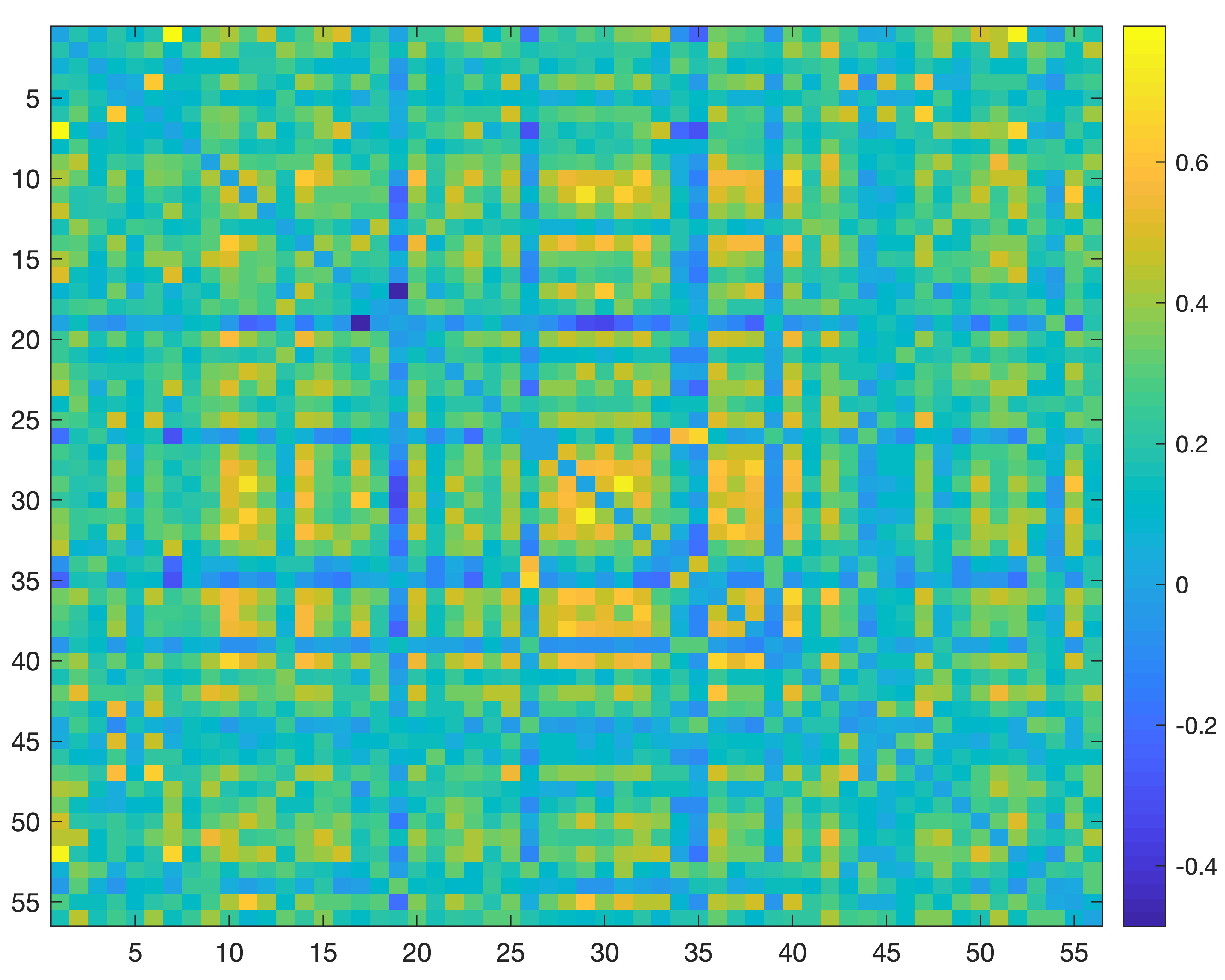
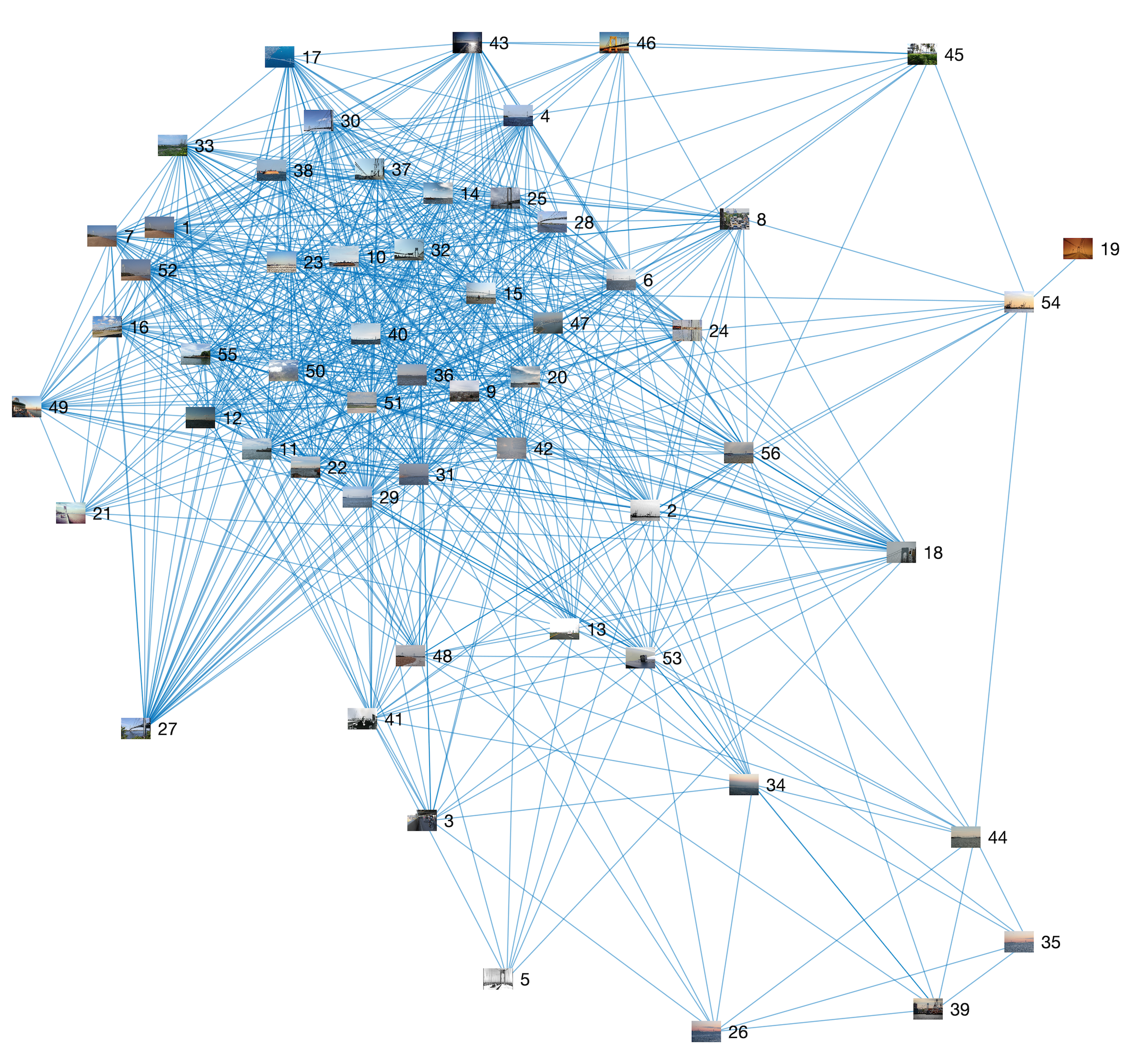
Figure 18 shows the group of most similar images and Figure 19 shows the most dissimilar image pair in this class, according to the SSIM measure. Analyzing the similarity matrix reveals that the right image in Figure 19 is the most isolated image in the class.

Figure 18. Group of most similar images in the class (images 1,7, and 52 in the graphical model shown in Figure 17).

Figure 19. Most dissimilar images in the class of Verrazzano-Narrows bridge (images 17(left) and 19(right) in the graphical model). The image on the right is also the most isolated image in the class, based on the similarity matrix.

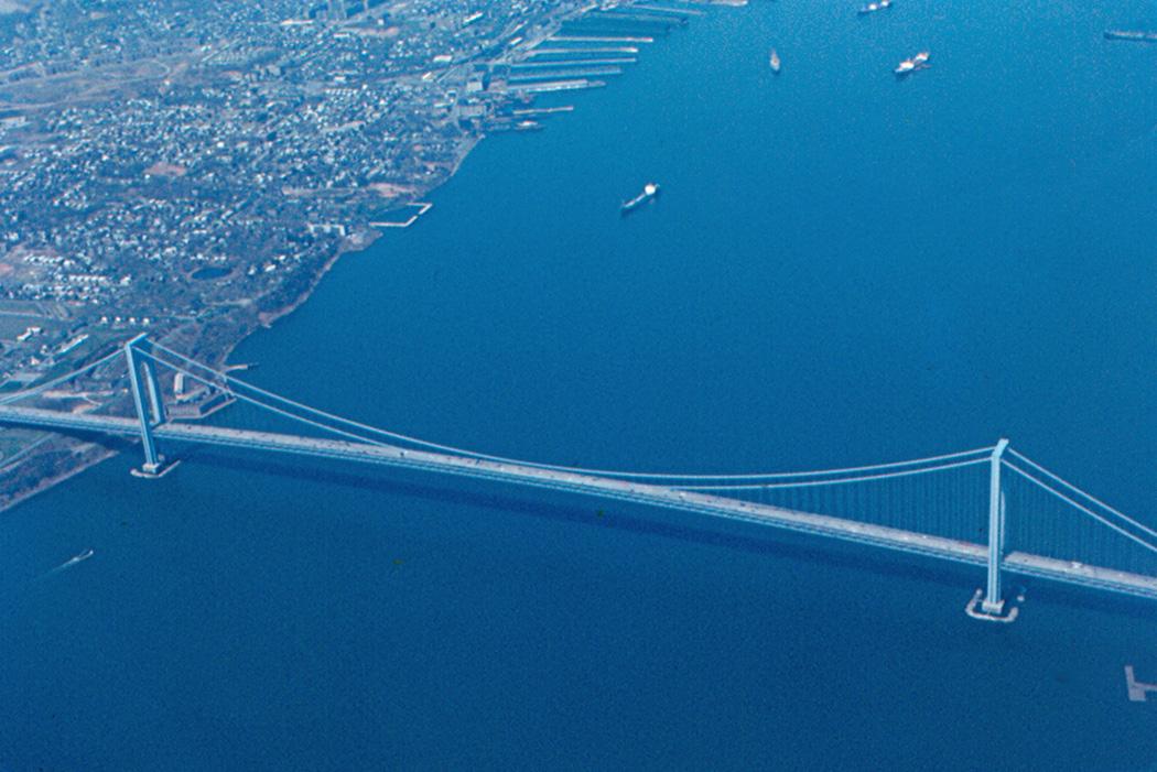
We note that our analysis has made us familiar with images in this class and provided us with insights about their similarities and differences. We know which training images might be redundant and which image might be an anomaly. In the case of active learning, we can try to fill the gaps in training data according to the graphical model shown in Figure 17.

7. Conclusions and future work

We developed a set of efficient tools for analyzing images in training sets. We showed that similar images in standard image classification datasets can be identified easy and fast, prior to training a model on them. We showed that performing this types of analysis on training and also testing sets can provide useful insights about the datasets and also the models trained on them. For example, one can quickly find redundant and influential images. By analyzing the eigen-gaps of a graph Laplacian, one can estimate the percentage of redundancies in a dataset, useful for many real world datasets.

Our method eases the computational cost barrier for analyzing the contents of image-classification datasets and therefore makes it practical for users to closely engage with the datasets and learn useful insights about their contents and their fine-level details.

Possible extension of this work is to further study the similarities and differences across training and testing sets and use that information to explain the generalization of models. Further investigating the images in relation to decision boundaries of models, during and after training, may provide useful insights on how training images shape the models by defining their decision boundaries. Moreover, our methods have applications in the context of active learning.

References

- (1)
- Achille et al. (2019) Alessandro Achille, Michael Lam, Rahul Tewari, Avinash Ravichandran, Subhransu Maji, Charless C Fowlkes, Stefano Soatto, and Pietro Perona. 2019. Task2vec: Task embedding for meta-learning. In Proceedings of the IEEE International Conference on Computer Vision. 6430–6439.
- Alain et al. (2015) Guillaume Alain, Alex Lamb, Chinnadhurai Sankar, Aaron Courville, and Yoshua Bengio. 2015. Variance reduction in SGD by distributed importance sampling. arXiv preprint arXiv:1511.06481 (2015).
- Albanesi et al. (2018) Maria Grazia Albanesi, Riccardo Amadeo, Silvia Bertoluzza, and Giulia Maggi. 2018. A new class of wavelet-based metrics for image similarity assessment. Journal of Mathematical Imaging and Vision 60, 1 (2018), 109–127.
- Arora et al. (2019) Sanjeev Arora, Simon Du, Wei Hu, Zhiyuan Li, and Ruosong Wang. 2019. Fine-Grained Analysis of Optimization and Generalization for Overparameterized Two-Layer Neural Networks. In International Conference on Machine Learning. 322–332.
- Arora et al. (2018) Sanjeev Arora, Rong Ge, Behnam Neyshabur, and Yi Zhang. 2018. Stronger Generalization Bounds for Deep Nets via a Compression Approach. In International Conference on Machine Learning. 254–263.
- Arthur and Vassilvitskii (2007) David Arthur and Sergei Vassilvitskii. 2007. k-means++: The advantages of careful seeding. In Proceedings of the 18th Annual ACM-SIAM Symposium on Discrete Algorithms. 1027–1035.
- Barz and Denzler (2019) Björn Barz and Joachim Denzler. 2019. Do we train on test data? Purging CIFAR of near-duplicates. arXiv preprint arXiv:1902.00423 (2019).
- Belkin et al. (2018) Mikhail Belkin, Siyuan Ma, and Soumik Mandal. 2018. To Understand Deep Learning We Need to Understand Kernel Learning. In International Conference on Machine Learning. 541–549.
- Birodkar et al. (2019) Vighnesh Birodkar, Hossein Mobahi, and Samy Bengio. 2019. Semantic Redundancies in Image-Classification Datasets: The 10% You Don’t Need. arXiv preprint arXiv:1901.11409 (2019).
- Carlini et al. (2018) Nicholas Carlini, Ulfar Erlingsson, and Nicolas Papernot. 2018. Prototypical Examples in Deep Learning: Metrics, Characteristics, and Utility.
- Chan (1987) Tony F Chan. 1987. Rank revealing QR factorizations. Linear Algebra Appl. 88 (1987), 67–82.
- Chen et al. (2019) Chaofan Chen, Oscar Li, Alina Barnett, Jonathan Su, and Cynthia Rudin. 2019. This looks like that: Deep learning for interpretable image recognition. Advances in Neural Information Processing Systems (2019).
- Chitta et al. (2019) Kashyap Chitta, Jose M Alvarez, Elmar Haussmann, and Clement Farabet. 2019. Less is More: An Exploration of Data Redundancy with Active Dataset Subsampling. arXiv preprint arXiv:1905.12737 (2019).
- Chui (2016) Charles K Chui. 2016. An introduction to wavelets. Elsevier.
- Daubechies (1992) Ingrid Daubechies. 1992. Ten Lectures on Wavelets. Society for Industrial and Applied Mathematics, Philadelphia.
- Dong et al. (2019) Kun Dong, Austin R. Benson, and David Bindel. 2019. Network Density of States. In Proceedings of the 25th ACM SIGKDD International Conference on Knowledge Discovery & Data Mining (KDD ’19). ACM, 1152–1161.
- Elsayed et al. (2018) Gamaleldin Elsayed, Dilip Krishnan, Hossein Mobahi, Kevin Regan, and Samy Bengio. 2018. Large margin deep networks for classification. In Advances in Neural Information Processing Systems. 842–852.
- Fawzi et al. (2018) Alhussein Fawzi, Seyed-Mohsen Moosavi-Dezfooli, Pascal Frossard, and Stefano Soatto. 2018. Empirical study of the topology and geometry of deep networks. In Proceedings of the IEEE Conference on Computer Vision and Pattern Recognition. 3762–3770.
- Golub and Van Loan (2012) Gene H Golub and Charles F Van Loan. 2012. Matrix Computations (4th ed.). JHU Press, Baltimore.
- Guo and Schuurmans (2008) Yuhong Guo and Dale Schuurmans. 2008. Discriminative batch mode active learning. In Advances in Neural Information Processing Systems. 593–600.
- He et al. (2016) Kaiming He, Xiangyu Zhang, Shaoqing Ren, and Jian Sun. 2016. Identity mappings in deep residual networks. In European conference on computer vision. Springer, 630–645.
- Huang et al. (2019) W Ronny Huang, Zeyad Emam, Micah Goldblum, Liam Fowl, Justin K Terry, Furong Huang, and Tom Goldstein. 2019. Understanding generalization through visualizations. arXiv preprint arXiv:1906.03291 (2019).
- Jiang et al. (2019) Yiding Jiang, Dilip Krishnan, Hossein Mobahi, and Samy Bengio. 2019. Predicting the Generalization Gap in Deep Networks with Margin Distributions. In International Conference on Learning Representations (ICLR 2019).
- Katharopoulos and Fleuret (2018) Angelos Katharopoulos and Francois Fleuret. 2018. Not All Samples Are Created Equal: Deep Learning with Importance Sampling. In International Conference on Machine Learning. 2530–2539.
- Kim et al. (2014) Been Kim, Cynthia Rudin, and Julie A Shah. 2014. The bayesian case model: A generative approach for case-based reasoning and prototype classification. In Advances in Neural Information Processing Systems. 1952–1960.
- Koh et al. (2019) Pang Wei Koh, Kai-Siang Ang, Hubert HK Teo, and Percy Liang. 2019. On the Accuracy of Influence Functions for Measuring Group Effects. arXiv preprint arXiv:1905.13289 (2019).
- Koh and Liang (2017) Pang Wei Koh and Percy Liang. 2017. Understanding Black-box Predictions via Influence Functions. In International Conference on Machine Learning (ICML 2017). 1885–1894.
- Kolesnikov et al. (2019) Alexander Kolesnikov, Lucas Beyer, Xiaohua Zhai, Joan Puigcerver, Jessica Yung, Sylvain Gelly, and Neil Houlsby. 2019. Large Scale Learning of General Visual Representations for Transfer. arXiv preprint arXiv:1912.11370 (2019).
- Krizhevsky et al. (2009) Alex Krizhevsky, Geoffrey Hinton, et al. 2009. Learning multiple layers of features from tiny images. Technical Report. Citeseer.
- Kutyniok and Labate (2012) Gitta Kutyniok and Demetrio Labate. 2012. Shearlets: Multiscale analysis for multivariate data. Springer Science & Business Media.
- Lapedriza et al. (2013) Agata Lapedriza, Hamed Pirsiavash, Zoya Bylinskii, and Antonio Torralba. 2013. Are all training examples equally valuable? arXiv preprint arXiv:1311.6510 (2013).
- Li et al. (2020) Jingling Li, Yanchao Sun, Jiahao Su, Taiji Suzuki, and Furong Huang. 2020. Understanding Generalization in Deep Learning via Tensor Methods. arXiv preprint arXiv:2001.05070 (2020).
- Li et al. (2018) Oscar Li, Hao Liu, Chaofan Chen, and Cynthia Rudin. 2018. Deep Learning for Case-based Reasoning through Prototypes: A Neural Network that Explains its Predictions. In Proceedings of AAAI Conference on Artificial Intelligence.
- Lloyd (1982) Stuart Lloyd. 1982. Least squares quantization in PCM. IEEE Transactions on Information Theory 28, 2 (1982), 129–137.
- Loshchilov and Hutter (2015) Ilya Loshchilov and Frank Hutter. 2015. Online batch selection for faster training of neural networks. arXiv preprint arXiv:1511.06343 (2015).
- Loupias et al. (2000) Etienne Loupias, Nicu Sebe, Stéphane Bres, and J-M Jolion. 2000. Wavelet-based salient points for image retrieval. In Proceedings 2000 International Conference on Image Processing (Cat. No. 00CH37101), Vol. 2. IEEE, 518–521.
- Meletis et al. (2019) Panagiotis Meletis, Rob Romijnders, and Gijs Dubbelman. 2019. Data Selection for training Semantic Segmentation CNNs with cross-dataset weak supervision. arXiv preprint arXiv:1907.07023 (2019).
- Newman (2004) Mark EJ Newman. 2004. Fast algorithm for detecting community structure in networks. Physical review E 69, 6 (2004), 066133.
- Noh et al. (2017) Hyeonwoo Noh, Andre Araujo, Jack Sim, Tobias Weyand, and Bohyung Han. 2017. Large-scale image retrieval with attentive deep local features. In Proceedings of the IEEE International Conference on Computer Vision. 3456–3465.
- Ohno-Machado et al. (1998) Lucila Ohno-Machado, Hamish S Fraser, and A Ohrn. 1998. Improving machine learning performance by removing redundant cases in medical data sets.. In Proceedings of the AMIA Symposium. American Medical Informatics Association, 523.
- Reisenhofer et al. (2018) Rafael Reisenhofer, Sebastian Bosse, Gitta Kutyniok, and Thomas Wiegand. 2018. A Haar wavelet-based perceptual similarity index for image quality assessment. Signal Processing: Image Communication 61 (2018), 33–43.
- Sampat et al. (2009) Mehul P Sampat, Zhou Wang, Shalini Gupta, Alan Conrad Bovik, and Mia K Markey. 2009. Complex wavelet structural similarity: A new image similarity index. IEEE Transactions on Image Processing 18, 11 (2009), 2385–2401.
- Sankararaman et al. (2019) Karthik A Sankararaman, Soham De, Zheng Xu, W Ronny Huang, and Tom Goldstein. 2019. The impact of neural network overparameterization on gradient confusion and stochastic gradient descent. arXiv preprint arXiv:1904.06963 (2019).
- Tschandl et al. (2018) Philipp Tschandl, Cliff Rosendahl, and Harald Kittler. 2018. The HAM10000 dataset, a large collection of multi-source dermatoscopic images of common pigmented skin lesions. Scientific data 5 (2018), 180161.
- Vo et al. (2019) Huy V Vo, Francis Bach, Minsu Cho, Kai Han, Yann LeCun, Patrick Pérez, and Jean Ponce. 2019. Unsupervised image matching and object discovery as optimization. In Proceedings of the IEEE Conference on Computer Vision and Pattern Recognition. 8287–8296.
- Vodrahalli et al. (2018) Kailas Vodrahalli, Ke Li, and Jitendra Malik. 2018. Are all training examples created equal? An empirical study. arXiv preprint arXiv:1811.12569 (2018).
- von Luxburg (2007) Ulrike von Luxburg. 2007. A tutorial on spectral clustering. Statistics and Computing 17, 4 (2007), 395–416.
- Wang et al. (2004) Zhou Wang, Alan C Bovik, Hamid R Sheikh, Eero P Simoncelli, et al. 2004. Image quality assessment: From error visibility to structural similarity. IEEE transactions on image processing 13, 4 (2004), 600–612.
- Wang and Simoncelli (2005) Zhou Wang and Eero P Simoncelli. 2005. Translation insensitive image similarity in complex wavelet domain. In Proceedings of IEEE International Conference on Acoustics, Speech, and Signal Processing, Vol. 2. IEEE, 573–576.
- Yousefzadeh (2019) Roozbeh Yousefzadeh. 2019. Interpreting Machine Learning Models and Application of Homotopy Methods. Ph.D. Dissertation. University of Maryland, College Park.
- Yousefzadeh and O’Leary (2019a) Roozbeh Yousefzadeh and Dianne P O’Leary. 2019a. Investigating Decision Boundaries of Trained Neural Networks. arXiv preprint arXiv:1908.02802 (2019).
- Yousefzadeh and O’Leary (2019b) Roozbeh Yousefzadeh and Dianne P O’Leary. 2019b. Refining the Structure of Neural Networks Using Matrix Conditioning. arXiv preprint arXiv:1908.02400 (2019).
- Yousefzadeh and O’Leary (2020) Roozbeh Yousefzadeh and Dianne P O’Leary. 2020. Deep Learning Interpretation: Flip Points and Homotopy Methods, In Mathematical and Scientific Machine Learning Conference (MSML 2020). arXiv preprint arXiv:1903.08789.
- Zhang et al. (2016) Chiyuan Zhang, Samy Bengio, Moritz Hardt, Benjamin Recht, and Oriol Vinyals. 2016. Understanding deep learning requires rethinking generalization. arXiv preprint arXiv:1611.03530 (2016).
- Zujovic et al. (2013) Jana Zujovic, Thrasyvoulos N Pappas, and David L Neuhoff. 2013. Structural texture similarity metrics for image analysis and retrieval. IEEE Transactions on Image Processing 22, 7 (2013), 2545–2558.