Being Bayesian, Even Just a Bit,
Fixes Overconfidence in ReLU Networks

Abstract

The point estimates of ReLU classification networks—arguably the most widely used neural network architecture—have been shown to yield arbitrarily high confidence far away from the training data. This architecture, in conjunction with a maximum a posteriori estimation scheme, is thus not calibrated nor robust. Approximate Bayesian inference has been empirically demonstrated to improve predictive uncertainty in neural networks, although the theoretical analysis of such Bayesian approximations is limited. We theoretically analyze approximate Gaussian distributions on the weights of ReLU networks and show that they fix the overconfidence problem. Furthermore, we show that even a simplistic, thus cheap, Bayesian approximation, also fixes these issues. This indicates that a sufficient condition for a calibrated uncertainty on a ReLU network is “to be a bit Bayesian”. These theoretical results validate the usage of last-layer Bayesian approximation and motivate a range of a fidelity-cost trade-off. We further validate these findings empirically via various standard experiments using common deep ReLU networks and Laplace approximations.

1 Introduction

As neural networks have been successfully applied in ever more domains, including safety-critical ones, the robustness and uncertainty quantification of their predictions have moved into focus, subsumed under the notion of AI safety (Amodei et al., 2016). A principal goal of uncertainty quantification is that learning machines and neural networks in particular, should assign low confidence to test cases not explained well by the training data or prior information (Gal, 2016). The most obvious cases are test points that lie “far away” from the training data. Many methods to achieve this goal have been proposed, both Bayesian (e.g. Blundell et al., 2015; Louizos & Welling, 2017; Zhang et al., 2018) and non-Bayesian (e.g. Lakshminarayanan et al., 2017; Liang et al., 2018; Hein et al., 2019).

ReLU networks are currently among the most widely used neural architectures. This class comprises any network that can be written as a composition of linear layers (including fully-connected, convolutional, and residual layers) and a ReLU activation function. But, while ReLU networks often achieve high accuracy, the uncertainty of their predictions has been shown to be miscalibrated (Guo et al., 2017). Indeed, Hein et al. (2019) demonstrated that ReLU networks are always overconfident “far away from the data”: scaling a training point $\mathbf{x}$ (a vector in a Euclidean input space) with a scalar $\delta$ yields predictions of arbitrarily high confidence in the limit $\delta\to\infty$. This means ReLU networks are susceptible to out-of-distribution (OOD) examples. Meanwhile, probabilistic methods (in particular Bayesian methods) have long been known empirically to improve predictive uncertainty estimates. MacKay (1992a) demonstrated experimentally that the predictive uncertainty of Bayesian neural networks will naturally be high in regions not covered by training data. Although the theoretical analysis is still lacking, results like this raise the hope that the overconfidence problem of ReLU networks, too, might be mitigated by the use of probabilistic and Bayesian methods.

(a)

(b)

(c)

(d)

(e)

(a) MAP

(b) Temp. scaling

(c) Bayesian (last-layer)

(d) Bayesian (all-layer)

(e)

Figure 1: Binary classification on a toy dataset using a MAP estimate, temperature scaling, and both last-layer and all-layer Gaussian approximations over the weights which are obtained via Laplace approximations. Background color and black line represent confidence and decision boundary, respectively. Bottom row shows a zoomed-out view of the top row. The Bayesian approximations—even in the last-layer case—give desirable uncertainty estimates: confident close to the training data and uncertain otherwise. MAP and temperature scaling yield overconfident predictions. The optimal temperature is picked as in Guo et al. (2017).

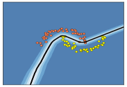
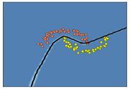
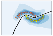
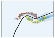
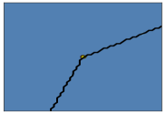
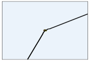
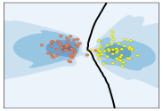
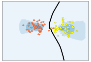
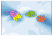
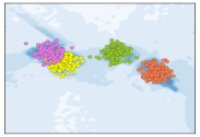
This paper offers a theoretical analysis of the binary classification case of ReLU networks with a logistic output layer. We show that equipping such networks with a Gaussian approximate distribution over the weights mitigates the aforementioned theoretical problem, in the sense that the predictive confidence far away from the training data approaches a known limit, bounded away from one, whose value is controlled by the covariance. In the case of Laplace approximations (MacKay, 1992b; Ritter et al., 2018), this treatment in conjunction with the probit approximation (Spiegelhalter & Lauritzen, 1990; MacKay, 1992a) does not change the decision boundary of the trained network, so it has no negative effect on the predictive performance (cf. Figure 1). Furthermore, we show that a sufficient condition for this desirable property to hold is to apply a Gaussian approximation only to the last layer of a ReLU network. This motivates the commonly used approximation scheme where an $L$-layer network is decomposed into a fixed feature map composed by the first $L-1$ layers and a Bayesian linear classifier (Gelman et al., 2008; Wilson et al., 2016a; Riquelme et al., 2018; Ober & Rasmussen, 2019; Brosse et al., 2020, etc.). This particular result implies that just being “a bit” Bayesian—at low cost overhead—already gives desirable benefits.

We empirically validate our results through various Laplace approximations on common deep ReLU networks. Furthermore, while our theoretical analysis is focused on the binary classification case, we also experimentally show that these Bayesian approaches yield good performance in the multi-class classification setting, suggesting that our analysis may carry over to this case.

To summarize, our contributions are three-fold:

1. we provide theoretical analysis on why ReLU networks equipped with Gaussian distributions over the weights mitigate the overconfidence problem in the binary classification setting,

2. we show that a sufficient condition for having this property is to be “a bit” Bayesian: employing a last-layer Gaussian approximation—in particular a Bayesian one, and

3. we validate our theoretical findings via a series of comprehensive experiments involving commonly-used deep ReLU networks and Laplace approximations in both binary and multi-class cases.

Section 2 begins with definitions, assumptions, and the problem statement, then develops the main theoretical results. Proofs are available in Appendix A. We discuss related work in Section 3, while empirical results are shown in Section 4.

2 Analysis

2.1 Preliminaries

Definitions

We call a function $f:\mathbb{R}^{n}\to\mathbb{R}^{k}$ piecewise affine if there exists a finite set of polytopes $\{Q_{r}\}_{r=1}^{R}$, referred to as the linear regions of $f$, such that $\cup_{r=1}^{R}Q_{r}=\mathbb{R}^{n}$ and $f|_{Q_{r}}$ is an affine function for every $Q_{r}$. ReLU networks are networks that result in piecewise affine classifier functions (Arora et al., 2018), which include networks with fully-connected, convolutional, and residual layers where just ReLU or leaky-ReLU are used as activation functions and max or average pooling are used in convolution layers. Let $\mathcal{D}:=\{\mathbf{x}_{i}\in\mathbb{R}^{n},t_{i}\}_{i=1}^{m}$ be a dataset, where the targets are $t_{i}\in\{0,1\}$ or $t_{i}\in\{1,\dots,k\}$ for the binary and multi-class case, respectively. Let $\phi:\mathbb{R}^{n}\to\mathbb{R}^{d}$ be an arbitrary fixed feature map and write $\bm{\phi}:=\phi(\mathbf{x})$ for a given $\mathbf{x}$. We define the logistic (sigmoid) function as $\sigma(z):=1/(1+\exp(-z))$ for $z\in\mathbb{R}$ and the softmax function as $\mathrm{softmax}(\mathbf{z},i):=\exp(z_{i})/\sum_{j}\exp(z_{j})$ for $\mathbf{z}\in\mathbb{R}^{k}$ and $i\in\{1,\dots,k\}$. Given a neural network $f_{\bm{\theta}}$, we consider the distribution $p({\bm{\theta}}|\mathcal{D})$ over its parameters. Note that even though we use the notation $p({\bm{\theta}}|\mathcal{D})$, we do not require this distribution to be a posterior distribution in the Bayesian sense. The predictive distribution for the binary case is

$$p(y=1|\mathbf{x},\mathcal{D}) =\int\sigma(f_{\bm{\theta}}(\mathbf{x}))\,p({\bm{\theta}}|\mathcal{D})\,d{\bm{\theta}}\,,$$ (1)

and for the multi-class case

$$p(y=i|\mathbf{x},\mathcal{D}) =\int\mathrm{softmax}(f_{\bm{\theta}}(\mathbf{x}),i)\,p({\bm{\theta}}|\mathcal{D})\,d{\bm{\theta}}\,.$$ (2)

The functions $\lambda_{i}(\cdot),\lambda_{\text{max}}(\cdot)$, and $\lambda_{\text{min}}(\cdot)$ return the $i$th, maximum, and minimum eigenvalue (which are assumed to exist) of their matrix argument, respectively. Similarly for the function $s_{i}(\cdot)$, $s_{\text{max}}(\cdot)$, and $s_{\text{min}}(\cdot)$ which return singular values instead. Finally, we assume that $\|\cdot\|$ is the $\ell^{2}$ norm.

Problem statement

The following theorem from Hein et al. (2019) shows that ReLU networks exhibit arbitrarily high confidence far away from the training data: If a point $\mathbf{x}\in\mathbb{R}^{n}$ is scaled by a sufficiently large scalar $\delta>0$, the input $\delta\mathbf{x}$ attains arbitrarily high confidence.

Theorem 2.1 (Hein et al., 2019).

Let $\mathbb{R}^{d}=\cup^{R}_{r=1}Q_{r}$ and $f|_{Q_{r}}(\mathbf{x})={\mathbf{U}}_{r}\mathbf{x}+{\mathbf{c}}_{r}$ be the piecewise affine representation of the output of a ReLU network on $Q_{r}$. Suppose that ${\mathbf{U}}_{r}$ does not contain identical rows for all $r=1,\dots,R$, then for almost any $\mathbf{x}\in\mathbb{R}^{n}$ and any $\epsilon>0$, there exists a $\delta>0$ and a class $i\in\{1,\dots,k\}$ such that it holds $\mathrm{softmax}(f(\delta\mathbf{x}),i)\geq 1-\epsilon$. Moreover, $\lim_{\delta\to\infty}\mathrm{softmax}(f(\delta\mathbf{x}),i)=1$. ∎

It is standard to treat neural networks as probabilistic models of the conditional distribution $p(y|\mathbf{x},{\bm{\theta}})$ over the prediction $y$. In this case, we define the confidence of any input point $\mathbf{x}$ as the maximum predictive probability, which in the case of a binary problem, can be written as $\max_{i\in\{0,1\}}\,p(y=i|\mathbf{x},{\bm{\theta}})=\sigma(|f_{\bm{\theta}}(\mathbf{x})|)$. Standard training involves assigning a maximum a posteriori (MAP) estimate ${\bm{\theta}}_{\text{MAP}}$ to the weights, ignoring potential uncertainty on ${\bm{\theta}}$. We will show that this lack of uncertainty is the primary cause of the overconfidence discussed by Hein et al. (2019) and argue that it can be mitigated by considering the marginalized prediction in (1) instead.

Even for a linear classifier parametrized by a single weight matrix ${\bm{\theta}}=\mathbf{w}$, there is generally no analytic solution for (1). But, good approximations exist when the distribution over the weights is a Gaussian $p(\mathbf{w}|\mathcal{D})\approx\mathcal{N}(\mathbf{w}|{\bm{\mu}},\mathbf{\Sigma})$ with mean ${\bm{\mu}}$ and covariance $\mathbf{\Sigma}$. One such approximation (Spiegelhalter & Lauritzen, 1990; MacKay, 1992a) is constructed by scaling the input of the probit function $\Phi$ by a constant $\lambda=\sqrt{\pi/8}$ . Using this approximation and the Gaussian assumption, if we let $a:=\mathbf{w}^{\top}\bm{\phi}$, we get

$$p(y=1|\mathbf{x},\mathcal{D}) \approx\int\Phi(\sqrt{\pi/8}\,a)\,\mathcal{N}(a|{\bm{\mu}}^{\top}\bm{\phi},\bm{\phi}^{\top}\mathbf{\Sigma}\bm{\phi})\,da$$

$$=\Phi\left(\frac{{\bm{\mu}}^{\top}\bm{\phi}}{\sqrt{8/\pi+\bm{\phi}^{\top}\mathbf{\Sigma}\bm{\phi}}}\right)\approx\sigma\left(z(\mathbf{x})\right)\,,$$ (3)

where the last step uses the approximation $\Phi(\sqrt{\pi/8}\,x)\approx\sigma(x)$ a second time, with

$$z(\mathbf{x}):=\frac{{\bm{\mu}}^{\top}\bm{\phi}}{\sqrt{1+\pi/8\,\bm{\phi}^{\top}\mathbf{\Sigma}\bm{\phi}}}\,.$$ (4)

In the case of ${\bm{\mu}}=\mathbf{w}_{\text{MAP}}$, Section 2.1 can be seen as the “softened” version of the MAP prediction of the classifier, using the covariance of the Gaussian. The confidence in this case is $\max_{i\in\{0,1\}}\,p(y=i|\mathbf{x},\mathcal{D})=\sigma(|z(\mathbf{x})|)$.

We can generalize the previous insight to the case where the parameters of the feature map $\phi$ are also approximated by a Gaussian. Let ${\bm{\theta}}\in\mathbb{R}^{p}$ be the parameter vector of a NN $f_{\bm{\theta}}:\mathbb{R}^{n}\to\mathbb{R}$ with a given Gaussian approximation $p({\bm{\theta}}|\mathcal{D})\approx\mathcal{N}({\bm{\theta}}|{\bm{\mu}},{\bm{\Sigma}})$. Let $\mathbf{x}\in\mathbb{R}^{n}$ be an arbitrary input point. Letting ${\mathbf{d}}:=\nabla f_{\bm{\theta}}(\mathbf{x})|_{\bm{\mu}}$, we do a first-order Taylor expansion of $f_{\bm{\theta}}$ at ${\bm{\mu}}$ (MacKay, 1995): $f_{\bm{\theta}}(\mathbf{x})\approx f_{\bm{\mu}}(\mathbf{x})+{\mathbf{d}}^{\top}({\bm{\theta}}-{\bm{\mu}})$. This implies that the distribution over $f_{\bm{\theta}}(\mathbf{x})$ is given by $p(f_{\bm{\theta}}(\mathbf{x})|\mathbf{x},\mathcal{D})\approx\mathcal{N}(f_{\bm{\theta}}(\mathbf{x})|f_{\bm{\mu}}(\mathbf{x}),{\mathbf{d}}^{\top}{\bm{\Sigma}}{\mathbf{d}})$. Therefore, we have

$$z(\mathbf{x}):=\frac{f_{\bm{\mu}}(\mathbf{x})}{\sqrt{1+\pi/8\,{\mathbf{d}}^{\top}{\bm{\Sigma}}{\mathbf{d}}}}\,.$$ (5)

It is easy to see that (4) is indeed a special case of (5).

As the first notable property of this approximation, we show that, in contrast to some other methods for uncertainty quantification (e.g. Monte Carlo dropout, Gal & Ghahramani, 2016) it preserves the decision boundary induced by the MAP estimate.

Proposition 2.2 (Invariance property).

Let $f_{\bm{\theta}}:\mathbb{R}^{n}\to\mathbb{R}$ be a binary classifier network parametrized by ${\bm{\theta}}$ and let $\mathcal{N}({\bm{\theta}}|{\bm{\mu}},\mathbf{\Sigma})$ be the distribution over ${\bm{\theta}}$. Then for any $\mathbf{x}\in\mathbb{R}^{n}$, we have $\sigma(f_{{\bm{\mu}}}(\mathbf{x}))=0.5$ if and only if $\sigma(z(\mathbf{x}))=0.5$.

This property is useful in practice, particularly whenever ${\bm{\mu}}={\bm{\theta}}_{\text{MAP}}$, since it guarantees that employing a Gaussian approximation on top of a MAP-trained network will not reduce the original classification accuracy. Virtually all state-of-the-art models in deep learning are trained via MAP estimation and sacrificing the classification performance that makes them attractive in the first place would be a waste.

2.2 Main Results

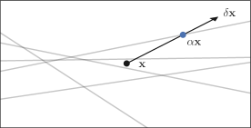
As our central theoretical contribution, we show that for any $\mathbf{x}\in\mathbb{R}^{n}$, as $\delta\to\infty$, the value of $|z(\delta\mathbf{x})|$ in (5) goes to a quantity that only depends on the mean and covariance of the Gaussian over the weights. Moreover, this property also holds in the finite asymptotic regime, far enough from the training data. This result implies that one can drive the confidence closer to the uniform (one-half) far away from the training points by shifting $|z(\mathbf{x})|$ closer to zero by controlling the Gaussian. We formalize this result in the following theorem. The situation is illustrated in Figure 2.

Theorem 2.3 (All-layer approximation).

Let $f_{\bm{\theta}}:\mathbb{R}^{n}\to\mathbb{R}$ be a binary ReLU classification network parametrized by ${\bm{\theta}}\in\mathbb{R}^{p}$ with $p\geq n$, and let $\mathcal{N}({\bm{\theta}}|{\bm{\mu}},\mathbf{\Sigma})$ be the Gaussian approximation over the parameters. Then for any input $\mathbf{x}\in\mathbb{R}^{n}$,

$$\lim_{\delta\to\infty}\sigma(|z(\delta\mathbf{x})|)\leq\sigma\left(\frac{\|{\mathbf{u}}\|}{s_{\text{\emph{min}}}\left({\mathbf{J}}\right)\sqrt{\pi/8\,\lambda_{\text{\emph{min}}}(\mathbf{\Sigma})}}\right)\,,$$ (6)

where ${\mathbf{u}}\in\mathbb{R}^{n}$ is a vector depending only on ${\bm{\mu}}$ and the $n\times p$ matrix ${\mathbf{J}}:=\left.\frac{\partial{\mathbf{u}}}{\partial{\bm{\theta}}}\right\rvert_{\bm{\mu}}$ is the Jacobian of ${\mathbf{u}}$ w.r.t. ${\bm{\theta}}$ at ${\bm{\mu}}$. Moreover, if $f_{\bm{\theta}}$ has no bias parameters, then there exists $\alpha>0$ such that for any $\delta\geq\alpha$, we have that

$$\sigma(|z(\delta\mathbf{x})|)\leq\lim_{\delta\to\infty}\sigma(|z(\delta\mathbf{x})|)\,.$$

Figure 2: The situation in Theorems 2.3 and 2.4. The intersections of gray lines are the linear regions.

The following question is practically interesting: Do we have to construct a probabilistic (Gaussian) uncertainty to the whole ReLU network for the previous property (Theorem 2.3) to hold? Surprisingly, the answer is no. The following theorem establishes that a guarantee similar to Theorem 2.3, is feasible even if only the last layer’s weights are assigned a Gaussian distribution. This amounts to a form of Bayesian logistic regression, where the features are provided by the ReLU network.

Theorem 2.4 (Last-layer approximation).

Let $g:\mathbb{R}^{d}\to\mathbb{R}$ be a binary linear classifier defined by $g(\phi(\mathbf{x})):=\mathbf{w}^{\top}\phi(\mathbf{x})$ where $\phi:\mathbb{R}^{n}\to\mathbb{R}^{d}$ is a fixed ReLU network and let $\mathcal{N}(\mathbf{w}|{\bm{\mu}},\mathbf{\Sigma})$ be the Gaussian approximation over the last-layer’s weights. Then for any input $\mathbf{x}\in\mathbb{R}^{n}$,

$$\lim_{\delta\to\infty}\sigma(|z(\delta\mathbf{x})|)\leq\sigma\left(\frac{\|{\bm{\mu}}\|}{\sqrt{\pi/8\,\lambda_{\text{\emph{min}}}(\mathbf{\Sigma})}}\right)\,.$$ (7)

Moreover, if $\phi$ has no bias parameters, then there exists $\alpha>0$ such that for any $\delta\geq\alpha$, we have that

$$\sigma(|z(\delta\mathbf{x})|)\leq\lim_{\delta\to\infty}\sigma(|z(\delta\mathbf{x})|)\,.$$

(a)

(b)

(a) MAP

(b) Bayesian

Figure 3: Absolute logit—$|f_{{\bm{\theta}}_{\text{MAP}}}(\delta\mathbf{x})|$ for MAP and $|z(\delta\mathbf{x})|$ for Bayesian—and confidence of the toy dataset in Figure 1 as functions of $\delta$. Each plot shows the mean and $\pm 3$ standard deviation over the test set.

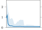
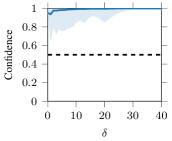
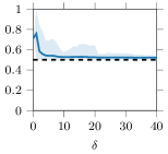
We show, using the same toy dataset and Gaussian-based last-layer Bayesian method as in Figure 1, an illustration of the previous results in Figure 3. Confirming the findings, for each input $\mathbf{x}$, the Gaussian approximation drives $|z(\delta\mathbf{x})|$ to a constant for sufficiently large $\delta$. Note that on true data points ($\delta=1$), the confidences remain high and the convergence occurs at some finite $\delta$.

Taken together, the results above formally validate the usage of the common Gaussian approximations of the weights distribution, both in Bayesian (MacKay, 1992b; Graves, 2011; Blundell et al., 2015, etc.) or non-Bayesian (Franchi et al., 2019; Lu et al., 2020, etc.) fashions, on ReLU networks for mitigating overconfidence problems. Furthermore, Theorem 2.4 shows that a full-blown Gaussian approximation or Bayesian treatment (i.e. on all layers of a NN) is not required to achieve control over the confidence far away from the training data. Put simply, even being “just a bit Bayesian” is enough to overcome at least asymptotic overconfidence.

We will show in the experiments (Section 4.3) that the same Bayesian treatment also mitigates asymptotic confidence in the multi-class case. However, extending the theoretical analysis to this case is not straightforward, even with analytic approximations such as those by Gibbs (1998) and Wu et al. (2019).

2.3 Laplace Approximations

The results in the previous section imply that the asymptotic confidence of a Gaussian-approximated binary ReLU classifier—either via a full or last-layer approximation—can be driven closer to uniform by controlling the covariance. In this section, we analyze the case when a Bayesian method in the form of a Laplace approximation is employed for obtaining the Gaussian. Although Laplace approximations are currently less popular than variational Bayes (VB), they have useful practical benefits: (i) they can be applied to any pre-trained network, (ii) whenever the approximation (5) can be employed, Proposition 2.2 holds, and (iii) no re-training is needed. Indeed, Laplace approximations can be attractive to practitioners who already have a working MAP-trained network, but want to enhance its uncertainty estimates further without decreasing performance.

The principle of Laplace approximations is as follows. Let $p({\bm{\theta}}|\mathcal{D})\propto p({\bm{\theta}})\prod_{\mathbf{x},t\in\mathcal{D}}p(y=t|\mathbf{x},{\bm{\theta}})$ be the posterior of a network $f_{\bm{\theta}}$. Then we can obtain a Gaussian approximation $p({\bm{\theta}}|\mathcal{D})\approx\mathcal{N}({\bm{\theta}}|{\bm{\mu}},\mathbf{\Sigma})$ of the posterior by setting ${\bm{\mu}}={\bm{\theta}}_{\text{MAP}}$ and $\mathbf{\Sigma}:=(-\nabla^{2}\log p({\bm{\theta}}|\mathcal{D})|_{{\bm{\theta}}_{\text{MAP}}})^{-1}$, the inverse Hessian of the negative log-posterior at the mode. In the binary classification case, the likelihood $p(y|\mathbf{x},\mathbf{w})$ is assumed to be a Bernoulli distribution $\mathcal{B}(\sigma(f_{\bm{\theta}}(\mathbf{x})))$. The prior $p({\bm{\theta}})$ is assumed to be an isotropic Gaussian $\mathcal{N}({\bm{\theta}}|\mathbf{0},\sigma^{2}_{0}\mathbf{I})$.

While the prior variance $\sigma^{2}_{0}$ is tied to the MAP estimation (it can be derived from the weight decay), it is often treated as a separate hyperparameter and tuned after training (Ritter et al., 2018). This treatment is useful in the case when one has only a pre-trained network and not the original training hyperparameters. Under this situation, in the following proposition, we analyze the effect of $\sigma^{2}_{0}$ on the asymptotic confidence presented by Theorem 2.3. The statement for the last-layer case is analogous and presented in Appendix A.

Proposition 2.5 (All-layer Laplace).

Let $f_{\bm{\theta}}$ be a binary ReLU classification network modeling a Bernoulli distribution $p(y|\mathbf{x},{\bm{\theta}})=\mathcal{B}(\sigma(f_{\bm{\theta}}(\mathbf{x})))$ with parameter ${\bm{\theta}}\in\mathbb{R}^{p}$. Let $\mathcal{N}({\bm{\theta}}|{\bm{\mu}},{\bm{\Sigma}})$ be the posterior obtained via a Laplace approximation with prior $\mathcal{N}({\bm{\theta}}|\mathbf{0},\sigma^{2}_{0}{\mathbf{I}})$, ${\mathbf{H}}$ be the Hessian of the negative log-likelihood at ${\bm{\mu}}$, and ${\mathbf{J}}$ be the Jacobian as in Theorem 2.3. Then for any input $\mathbf{x}\in\mathbb{R}^{n}$, the confidence $\sigma(|z(\mathbf{x})|)$ is a decreasing function of $\sigma^{2}_{0}$ with limits

$$\lim_{\sigma^{2}_{0}\to\infty}\sigma(|z(\mathbf{x})|) \leq\sigma\left(\frac{|f_{\bm{\mu}}(\mathbf{x})|}{1+\sqrt{\pi/8\,\lambda_{\text{\emph{max}}}({\mathbf{H}})\|{\mathbf{J}}\mathbf{x}\|^{2}}}\right)$$

$$\lim_{\sigma^{2}_{0}\to 0}\sigma(|z(\mathbf{x})|) =\sigma(|f_{\bm{\mu}}(\mathbf{x})|)\,.$$

The result above shows that the “far-away” confidence decreases (up to some limit) as the prior variance increases. Meanwhile, we recover the far-away confidence induced by the MAP estimate as the prior variance goes to zero. One could therefore pick a value of $\sigma_{0}^{2}$ as high as possible for mitigating overconfidence. However, this is undesirable since it also lowers the confidence of the training data and test data around them (i.e. the so-called in-distribution data), thus, causing underconfident predictions. Another common way to set this hyperparameter is by maximizing the validation log-likelihood (Ritter et al., 2018). This is also inadequate for our purpose since it only considers points close to the training data.

Inspired by Hendrycks et al. (2019) and Hein et al. (2019), we simultaneously prefer high confidence on the in-distribution validation set and low confidence (high entropy) on the out-of-distribution validation set. Let $\hat{\mathcal{D}}:=\{\hat{\mathbf{x}}_{i},\hat{t}_{i}\}_{i=1}^{m}$ be a validation set and $\tilde{\mathcal{D}}:=\{\tilde{\mathbf{x}}_{i}\}_{i=1}^{m}$ be an out-of-distribution dataset. We then pick the optimal $\sigma_{0}^{2}$ by solving the following one-parameter optimization problem:

$$\operatorname*{arg\,min}_{\sigma_{0}^{2}}-\frac{1}{m}\sum_{i=1}^{m}\log p(y=\hat{t}_{i}|\hat{\mathbf{x}}_{i},\mathcal{D})+\lambda H[p(y|\tilde{\mathbf{x}}_{i},\mathcal{D})]\,,$$ (8)

where $\lambda\in[0,1]$ is controlling the trade-off between both terms. The first term in (8) is the standard cross-entropy loss over $\hat{\mathcal{D}}$ while the second term is the negative predictive entropy over $\tilde{\mathcal{D}}$. Alternatively, the second term can be replaced by the cross-entropy loss where the target is the uniform probability vector. In all our experiments, we simply assume that $\tilde{\mathcal{D}}$ is a collection of uniform noise in the input space.

3 Related Work

(a)

(b)

(c)

(d)

(e)

(a) MAP

(b) Temp. scaling

(c) LLLA

(d) Full Laplace

(e)

Figure 4: Binary (top) and multi-class (bottom) toy classification problem. Background color represents confidence.

The overconfidence problem of deep neural networks, and thus ReLU networks, has long been known in the deep learning community (Nguyen et al., 2015), although a formal description was only delivered recently. Many methods have been proposed to combat or at least detect this issue. Post-hoc heuristics based on temperature or Platt scaling (Platt et al., 1999; Guo et al., 2017; Liang et al., 2018) are unable to detect inputs with arbitrarily high confidence far away from the training data (Hein et al., 2019).

Many works on uncertainty quantification in deep learning have recently been proposed. Gast & Roth (2018) proposed lightweight probabilistic networks via assumed density filtering. Malinin & Gales (2018, 2019); Sensoy et al. (2018) employ a Dirichlet distribution to model the distribution of a network’s output. Lakshminarayanan et al. (2017) quantify predictive uncertainty based on the idea of model ensembling and frequentist calibration. Hein et al. (2019) proposed enhanced training objectives based on robust optimization to mitigate this issue. Meinke & Hein (2020) proposed a similar approach with provable guarantees. However, they either lack in their theoretical analysis or do not employ probabilistic or Bayesian approximations. Our results, meanwhile, provide a theoretical justification to the commonly-used Gaussian approximations of NNs’ weights, both Bayesian (Graves, 2011; Blundell et al., 2015; Louizos & Welling, 2016; Maddox et al., 2019, etc.) and non-Bayesian (Franchi et al., 2019; Lu et al., 2020, etc.).

Bayesian methods have long been thought to mitigate the overconfidence problem on any neural network (MacKay, 1992a). Empirical evidence supporting this intuition has also been presented (Liu et al., 2019; Wu et al., 2019, etc.). Our results complement these with a theoretical justification for the ReLU-logistic case. Furthermore, our theoretical results show that, in some cases, an expensive Bayesian treatment over all layers of a network is not necessary (Theorem 2.4). Our results are thus theoretically validating the usage of Bayesian generalized linear models (Gelman et al., 2008) (especially in conjunction with ReLU features) and last-layer Bayesian methods (Snoek et al., 2015; Wilson et al., 2016a, b; Riquelme et al., 2018); and complementing the empirical analyses of Ober & Rasmussen (2019) and Brosse et al. (2020).

4 Experiments

(a)

(b)

(c)

(d)

(a)

(b)

(c)

(d)

(a) Bin.-MNIST

(b) Bin.-CIFAR10

(c) Bin.-SVHN

(d) Bin.-CIFAR100

Figure 5: Confidence of MAP (top row), temperature scaling (middle row), and LLLA (bottom row) as functions of $\delta$ over the test sets of binary classification datasets. Thick blue lines and shades correspond to means and $\pm 3$ standard deviations, respectively. Dashed lines signify the desirable confidence for $\delta$ sufficiently high.

Table 1: OOD detection for far-away points in binary classification settings. The in-distribution datasets are Binary-MNIST, Binary-CIFAR10, Binary-SVHN, and Binary-CIFAR100. Each OOD dataset is obtained by scaling uniform noise images in the corresponding input space of the in-distribution dataset with $\delta=100$. All values are means and standard deviations over 10 trials.

	MAP		+Temp.		+LLLA
	MMC $\downarrow$	AUR $\uparrow$	MMC $\downarrow$	AUR $\uparrow$	MMC $\downarrow$	AUR $\uparrow$
Binary-MNIST	99.9$\pm$0.0	-	100.0$\pm$0.0	-	79.4$\pm$0.9	-
Noise ($\delta=100$)	100.0$\pm$0.0	0.2$\pm$0.1	100.0$\pm$0.0	45.1$\pm$5.8	67.5$\pm$0.8	99.6$\pm$0.1
Binary-CIFAR10	96.3$\pm$0.3	-	90.5$\pm$0.6	-	76.4$\pm$0.3	-
Noise ($\delta=100$)	98.9$\pm$1.0	11.3$\pm$10.3	97.6$\pm$2.2	11.3$\pm$10.3	50.6$\pm$0.1	99.5$\pm$0.1
Binary-SVHN	99.4$\pm$0.0	-	98.2$\pm$0.1	-	80.7$\pm$0.1	-
Noise ($\delta=100$)	98.8$\pm$0.6	50.5$\pm$42.3	95.9$\pm$3.0	50.5$\pm$42.3	51.2$\pm$0.6	99.8$\pm$0.1
Binary-CIFAR100	94.5$\pm$0.5	-	74.5$\pm$2.9	-	66.7$\pm$0.5	-
Noise ($\delta=100$)	100.0$\pm$0.0	1.5$\pm$0.7	100.0$\pm$0.0	0.0$\pm$0.0	53.5$\pm$0.1	93.6$\pm$1.8

Table 2: Multi-class OOD detection results for MAP, last-layer Laplace (LLLA), (all-layers) diagonal Laplace (DLA), and (all-layers) Kronecker-Factored Laplace (KFLA). Each “far-away” Noise dataset is constructed as in Table 1 with $\delta=2000$. All values are averages and standard deviations over 10 trials.

	MAP		+Temp.		+LLLA		+DLA		+KFLA
	MMC $\downarrow$	AUR $\uparrow$	MMC $\downarrow$	AUR $\uparrow$	MMC $\downarrow$	AUR $\uparrow$	MMC $\downarrow$	AUR $\uparrow$	MMC $\downarrow$	AUR $\uparrow$
MNIST - MNIST	99.2$\pm$0.0	-	99.5$\pm$0.1	-	98.4$\pm$0.2	-	84.5$\pm$0.2	-	92.9$\pm$0.3	-
MNIST - EMNIST	82.3$\pm$0.0	89.2$\pm$0.1	87.6$\pm$1.4	88.9$\pm$0.2	70.2$\pm$1.9	92.0$\pm$0.4	54.5$\pm$0.3	87.7$\pm$0.4	58.7$\pm$0.4	89.6$\pm$0.3
MNIST - FMNIST	66.3$\pm$0.0	97.4$\pm$0.0	75.2$\pm$2.5	97.1$\pm$0.1	56.0$\pm$1.8	98.2$\pm$0.2	42.5$\pm$0.1	96.3$\pm$0.1	39.9$\pm$0.5	98.6$\pm$0.1
MNIST - Noise ($\delta=2000$)	100.0$\pm$0.0	0.1$\pm$0.0	100.0$\pm$0.0	6.8$\pm$4.1	99.9$\pm$0.0	9.6$\pm$0.7	84.9$\pm$1.3	53.7$\pm$3.1	55.6$\pm$2.0	97.3$\pm$0.4
CIFAR10 - CIFAR10	97.1$\pm$0.1	-	95.4$\pm$0.2	-	92.8$\pm$1.1	-	88.4$\pm$0.1	-	86.5$\pm$0.1	-
CIFAR10 - SVHN	62.5$\pm$0.0	95.8$\pm$0.1	54.6$\pm$0.6	96.1$\pm$0.0	45.9$\pm$1.6	96.4$\pm$0.1	43.3$\pm$0.1	95.5$\pm$0.1	43.0$\pm$0.1	94.8$\pm$0.1
CIFAR10 - LSUN	74.5$\pm$0.0	91.9$\pm$0.1	66.9$\pm$0.6	92.2$\pm$0.1	57.4$\pm$1.9	92.7$\pm$0.4	49.0$\pm$0.5	92.8$\pm$0.3	47.6$\pm$0.4	92.2$\pm$0.2
CIFAR10 - Noise ($\delta=2000$)	98.7$\pm$0.2	10.9$\pm$0.4	98.4$\pm$0.2	10.0$\pm$0.5	17.4$\pm$0.0	100.0$\pm$0.0	60.7$\pm$2.0	89.6$\pm$1.1	61.8$\pm$1.5	87.6$\pm$0.9
SVHN - SVHN	98.5$\pm$0.0	-	97.4$\pm$0.2	-	93.2$\pm$1.0	-	88.8$\pm$0.0	-	90.8$\pm$0.0	-
SVHN - CIFAR10	70.4$\pm$0.0	95.4$\pm$0.0	64.1$\pm$0.9	95.4$\pm$0.0	43.4$\pm$2.1	97.2$\pm$0.1	38.0$\pm$0.1	97.6$\pm$0.0	41.2$\pm$0.1	97.5$\pm$0.0
SVHN - LSUN	71.7$\pm$0.0	95.5$\pm$0.0	65.4$\pm$1.0	95.6$\pm$0.0	44.3$\pm$2.3	97.3$\pm$0.1	39.5$\pm$0.7	97.5$\pm$0.2	42.0$\pm$0.6	97.5$\pm$0.1
SVHN - Noise ($\delta=2000$)	98.7$\pm$0.1	11.9$\pm$0.6	98.4$\pm$0.1	11.0$\pm$0.6	27.5$\pm$0.1	99.6$\pm$0.0	60.8$\pm$1.6	92.8$\pm$0.6	62.4$\pm$2.0	94.0$\pm$0.5
CIFAR100 - CIFAR100	81.2$\pm$0.1	-	78.9$\pm$0.8	-	74.6$\pm$0.2	-	76.4$\pm$0.2	-	73.4$\pm$0.2	-
CIFAR100 - SVHN	53.5$\pm$0.0	78.8$\pm$0.1	49.2$\pm$1.2	79.2$\pm$0.1	42.7$\pm$0.3	80.4$\pm$0.2	46.0$\pm$0.1	79.6$\pm$0.2	41.4$\pm$0.1	80.1$\pm$0.2
CIFAR100 - LSUN	50.7$\pm$0.0	81.0$\pm$0.1	46.8$\pm$1.1	81.1$\pm$0.1	39.8$\pm$0.2	82.6$\pm$0.2	43.5$\pm$0.3	81.5$\pm$0.2	39.7$\pm$0.4	81.6$\pm$0.3
CIFAR100 - Noise ($\delta=2000$)	99.5$\pm$0.1	2.8$\pm$0.2	99.4$\pm$0.1	2.6$\pm$0.2	5.9$\pm$0.0	99.9$\pm$0.0	41.5$\pm$1.5	84.2$\pm$0.9	37.1$\pm$1.3	84.2$\pm$0.8

We corroborate our theoretical results via four experiments using various Gaussian-based Bayesian methods. In Section 4.1 we visualize the confidence of 2D binary and multi-class toy datasets. In Section 4.2 we empirically validate our main result that the confidence of binary classification datasets approaches finite constants as $\delta$ increases. Furthermore, we show empirically that this property also holds in the multi-class case, along with the usefulness of Bayesian methods in standard OOD detection tasks in Section 4.3. Finally, in Section 4.4, we show that our results also hold in the case of last-layer Gaussian processes.

Unless stated otherwise, we use LeNet (for MNIST) or ResNet-18 (for CIFAR-10, SVHN, CIFAR-100) architectures. We train these networks by following the procedure described by Meinke & Hein (2020) (LABEL:appendix:training). To obtain the optimal hyperparameter $\sigma_{0}^{2}$, we follow (8) with $\lambda$ set to 0.25. We mainly use a last-layer Laplace approximation (LLLA) where a Laplace approximation with an exact Hessian or its Kronecker factors is applied only to the last layer of a network (Appendix B). Whenever the approximations of predictive distribution in (4) and (5) cannot be used, we compute them via Monte Carlo integrations with 100 posterior samples. Other Laplace approximations that we use will be introduced in the subsection where they are first employed. Besides the vanilla MAP method, we use the temperature scaling method (Guo et al., 2017) as a baseline since it claims to give calibrated predictions in the frequentist sense. In particular, the optimal temperature is found via a validation log-likelihood maximization using PyCalib (Wenger et al., 2019). For each dataset that we use, we obtain a validation set via a random split from the respective test set. Lastly, all numbers reported in this section are averages along with their standard deviations over 10 trials.

4.1 Toy Dataset

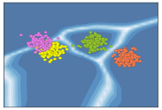
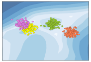
Here, the dataset is constructed by sampling the input points from $k$ independent Gaussians. The corresponding targets indicate from which Gaussian the point was sampled. We use a 3-layer ReLU network with 20 hidden units at each layer. We use the exact Hessian and the full generalized-Gauss-Newton (GGN) approximation of the Hessian for the case of LLLA and all-layer Laplace approximations, respectively.

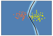
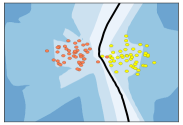
We show the results for the binary and multi-class cases in Figure 4. The MAP predictions have high confidence everywhere except at the region close to the decision boundary. Temperature scaling assigns low confidence to the training data, while assigning high confidence far away from them. LLLA, albeit simple, yields high confidence close to the training points and high uncertainty otherwise, while maintaining the MAP’s decision boundary. Furthermore, we found that the all-layer Laplace approximation makes the aforementioned finding stronger: the boundaries of the high-confidence regions are now closer to the training data.

4.2 Binary Classification

We validate our theoretical finding by plotting the test confidence of various binary classification datasets as functions of $\delta$. Each dataset is constructed by picking two classes which are most difficult to distinguish, based on the confusion matrix of the corresponding multi-class problem.

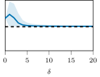
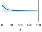
As shown in Figure 5, both MAP (top row) and temperature scaling (middle row) methods are overconfident for sufficiently large $\delta$. Meanwhile, LLLA which represents Bayesian methods, mitigates this issue: As $\delta$ increases, the confidence converges to some constant close to the uniform confidence (one-half). Moreover, when $\delta=1$ (the case of in-distribution data), LLLA retains higher confidence.

Table 1 further quantifies the results where we treat collections of 2000 uniform noise images scaled by $\delta=100$ as the OOD datasets. Note that, while the resulting data points are not in the image space anymore, this construction is useful to assess the effectiveness of the Bayesian methods in unbounded problems. We report the standard metrics proposed by Hendrycks & Gimpel (2017): mean-maximum-confidence (MMC) and area-under-ROC-curve (AUR). Confirming our finding in Figure 5, LLLA is able to detect OOD data with high accuracy: for the chosen values of $\delta$, the MMC and AUR values are close to the ideal values of 50 and 100, respectively. Both MAP and temperature scaling fail to do so since their confidence estimates saturate to one. These results (i) confirm our theoretical analysis in Section 2, (ii) show that even a simple Bayesian method yields good uncertainty estimates, and (iii) temperature scaling is not calibrated for outliers far-away from the training data.

4.3 Multi-class Classification

We also show empirically that Bayesian methods yield a similar behavior in multi-class settings. On top of LLLA, representing Bayesian methods, we employ various other scalable Laplace approximation techniques: diagonal Laplace approximation (DLA) where a diagonal Gaussian is used to approximate the posterior over all layers of a network, and Kronecker-factored Laplace approximation (KFLA) (Ritter et al., 2018) where a matrix-variate normal is used to approximate the posterior over all layers. We use 20 posterior samples for both DLA and KFLA. We refer the reader to Appendix B for details.

For each training dataset we evaluate all methods both in the non-asymptotic (the corresponding OOD test datasets, e.g. SVHN and LSUN for CIFAR-10) and asymptotic (Noise datasets) regime. Each “far-away” Noise dataset is constructed by scaling 2000 uniform noise images in the corresponding input space with $\delta=2000$. As in the previous section, we report the MMC and AUR metrics.

As presented in Table 2, all the Bayesian methods improve the OOD detection performance of the base models both in the non-asymptotic and asymptotic regime. Especially in the asymptotic regime, all the Bayesian methods perform well, empirically confirming our hypothesis that our theoretical analysis carries over to the multi-class setting. Meanwhile, both MAP’s and temperature scaling’s MMC and AUR are close to 100 and 0, respectively. Moreover, while LLLA is the simplest Bayesian method in this experiment, it often outperforms DLA and KFLA. Our finding agrees with the prior observation that last-layer Bayesian approximations are often sufficient (Ober & Rasmussen, 2019; Brosse et al., 2020). Furthermore, in LABEL:appendix:more_experiments we also show that we can apply Laplace approximations on top of prior OOD detection methods such as ACET (Hein et al., 2019) and Outlier-Exposure (Hendrycks et al., 2019) to achieve state-of-the-art performance in the non-asymptotic regime, while also having high uncertainty in the asymptotic regime.

Table 3: Wall-clock time (in second) of posterior inferences and predictions over test sets.

	MNIST	CIFAR-10	SVHN	CIFAR-100
Inference
MAP	-	-	-	-
+Temp.	0.0	0.0	0.0	0.0
+LLLA	1.8	23.0	33.7	23.1
+DLA	1.3	22.9	33.6	23.0
+KFLA	4.3	78.1	115.1	78.6
Prediction
MAP	0.4	1.2	2.7	1.2
+Temp.	0.4	1.2	2.7	1.2
+LLLA	0.9	1.7	4.3	1.6
+DLA	7.3	100.0	260.6	100.4
+KFLA	21.5	151.0	392.8	151.7

In Table 3, we present the computational cost analysis in terms of wall-clock time. We measure the time required for each method to do posterior inference (or finding the optimal temperature) and to make predictions. While MAP and temperature scaling are fast, as we have shown in the previous results, they are overconfident. Among the Bayesian methods, since the cost of LLLA is constant w.r.t. the network depth, we found that it is up to two orders of magnitude faster than DLA and KFLA when making predictions. All in all, this finding, combined with the previous results, makes this simple Bayesian method attractive in applications.

Table 4: Multi-class OOD detection results for deep kernel learning (DKL). Each “far-away” Noise dataset is constructed as in Table 2 with $\delta=2000$. All values are averages and standard deviations over 10 trials.

Train - Test	MMC $\downarrow$	AUR $\uparrow$
MNIST - MNIST	99.6$\pm$0.0	-
MNIST - EMNIST	83.9$\pm$0.0	94.4$\pm$0.1
MNIST - FMNIST	70.6$\pm$0.1	98.8$\pm$0.0
MNIST - Noise	58.6$\pm$0.5	99.7$\pm$0.0
CIFAR10 - CIFAR10	97.5$\pm$0.0	-
CIFAR10 - SVHN	50.6$\pm$0.1	98.6$\pm$0.0
CIFAR10 - LSUN	77.9$\pm$0.3	93.4$\pm$0.1
CIFAR10 - Noise	56.5$\pm$0.7	98.5$\pm$0.1
SVHN - SVHN	98.6$\pm$0.0	-
SVHN - CIFAR10	72.7$\pm$0.0	96.0$\pm$0.0
SVHN - LSUN	76.7$\pm$0.1	95.1$\pm$0.1
SVHN - Noise	48.6$\pm$0.7	99.4$\pm$0.0
CIFAR100 - CIFAR100	80.5$\pm$0.0	-
CIFAR100 - SVHN	72.7$\pm$0.1	63.1$\pm$0.1
CIFAR100 - LSUN	66.8$\pm$0.4	69.7$\pm$0.3
CIFAR100 - Noise	43.1$\pm$1.1	90.3$\pm$0.7

4.4 Last-layer Gaussian Processes

It has been shown that Gaussian-approximated linear models with infinitely many features, e.g. two-layer networks with infinitely wide hidden layers, are equivalent to Gaussian processes (Neal, 1996). In the language of Theorem 2.4, this is the case when the dimension of the feature space $\mathbb{R}^{d}$ goes to infinity. It is therefore interesting to see, at least empirically, whether low asymptotic confidence is also attained in this case.

While unlike LLLA, deep kernel learning (DKL, Wilson et al., 2016a, b) is not a post-hoc method, it is a suitable model for showcasing our theory in the case of last-layer Gaussian processes. We therefore train stochastic variational DKL models (Wilson et al., 2016b) which use the same networks used in the previous experiment (minus the top layer) as their feature extractors, following the implementation provided by GPyTorch (Gardner et al., 2018). The training protocol is identical as before (cf. LABEL:appendix:training). To compute each prediction, we use 20 samples from the Gaussian process posterior. We are mainly interested in the performance of DKL in term of multi-class OOD detection (both in asymptotic and non-asymptotic regimes), similar to the previous section.

The results are presented in Table 4. When compared to the results of the MAP estimation in Table 2, we found that DKL is able to mitigate asymptotic overconfidence (see results against the Noise dataset). These results empirically verify that our analysis also holds in the non-parametric infinite-width regime. Nevertheless, we found that LLLA generally outperforms DKL both in term of MMC and AUR metrics. This finding, along with the simplicity and efficiency of LLLA make it more attractive than DKL, especially since DKL requires retraining and thus cannot simply be applied to pre-trained ReLU networks.

5 Conclusion

We have shown analytically that Gaussian approximations of weights distributions, when applied on binary ReLU classification networks, can mitigate the asymptotic overconfidence problem that plagues deep learning. While this behavior does not seem surprising—indeed, Gaussian-based approximate Bayesian methods have empirically been known to give good uncertainty estimates—formal statements regarding this property had been missing. Our results provide some of these statements. Furthermore, we have shown, both theoretically and empirically, that a sufficient condition for good uncertainty estimates in ReLU networks is to be “a bit Bayesian”: apply a Gaussian-based probabilistic method, in particular a Bayesian one, to the last layer of the network. Our analysis further validates the common usage of approximate inference methods—both Bayesian and non-Bayesian—which leverage the Gaussian distribution.

Appendix A Proofs

In the followings, the norm $\|\cdot\|$ is the standard $\ell^{2}$-norm.

See 2.2

Proof.

Let $\mathbf{x}\in\mathbb{R}^{n}$ be arbitrary and denote $\mu_{f}:=f_{{\bm{\theta}}_{\text{MAP}}}(\mathbf{x})$ and $v_{f}:={\mathbf{d}}(\mathbf{x})^{\top}{\bm{\Sigma}}{\mathbf{d}}(\mathbf{x})$. For the forward direction, suppose that $\sigma(\mu_{f})=0.5$. This implies that $\mu_{f}=0$, and we have $\sigma(0/(1+\pi/8\,v_{f})^{1/2})=\sigma(0)=0.5$. For the reverse direction, suppose that $\sigma(\mu_{f}/(1+\pi/8\,v_{f})^{1/2})=0.5$. This implies $\mu_{f}/(1+\pi/8\,v_{f})^{1/2}=0$. Since the denominator of the l.h.s. is positive, it follows that $\mu_{f}$ must be $0$, implying that $\sigma(\mu_{f})=0.5$. ∎

Lemma A.1 (Hein et al., 2019).

Let $\{Q_{i}\}_{l=1}^{R}$ be the set of linear regions associated to the ReLU network $f:\mathbb{R}^{n}\to\mathbb{R}^{k}$. For any $\mathbf{x}\in\mathbb{R}^{n}$ there exists an $\alpha>0$ and $t\in\{1,\dots,R\}$ such that $\delta\mathbf{x}\in Q_{t}$ for all $\delta\geq\alpha$. Furthermore, the restriction of $f$ to $Q_{t}$ can be written as an affine function ${\mathbf{U}}^{\top}\mathbf{x}+{\mathbf{c}}$ for some suitable ${\mathbf{U}}\in\mathbb{R}^{n\times k}$ and ${\mathbf{c}}\in\mathbb{R}^{k}$. ∎

See 2.3

Proof.

By Lemma 3.1 of Hein et al. (2019) (also presented in Lemma A.1) there exists an $\alpha>0$ and a linear region $R$, along with $\mathbf{u}\in\mathbb{R}^{n}$ and $c\in\mathbb{R}$, such that for any $\delta\geq\alpha$, we have that $\delta\mathbf{x}\in R$ and the restriction $f_{\bm{\theta}}|_{R}$ can be written as ${\mathbf{u}}^{\top}\mathbf{x}+c$. Note that, for any such $\delta$, the vector ${\mathbf{u}}$ and scalar $c$ are constant w.r.t. $\delta\mathbf{x}$. Therefore for any such $\delta$, we can write the gradient ${\mathbf{d}}(\delta\mathbf{x})$ as follows:

$${\mathbf{d}}(\delta\mathbf{x}) =\left.\frac{\partial(\delta{\mathbf{u}}^{\top}\mathbf{x})}{\partial{\bm{\theta}}}\right|_{\bm{\mu}}+\left.\frac{\partial c}{\partial{\bm{\theta}}}\right|_{\bm{\mu}}=\left.\delta\frac{\partial{\mathbf{u}}}{\partial{\bm{\theta}}}\right|_{\bm{\mu}}^{\top}\mathbf{x}+\left.\frac{\partial c}{\partial{\bm{\theta}}}\right|_{\bm{\mu}}$$

$$=\delta\left({\mathbf{J}}^{\top}\mathbf{x}+\frac{1}{\delta}\nabla_{\bm{\theta}}\,c|_{\bm{\mu}}\right)\,.$$ (9)

Hence, by (5),

$$|z (\delta\mathbf{x})|=\frac{|\delta{\mathbf{u}}^{\top}\mathbf{x}+c|}{\sqrt{1+\pi/8\,{\mathbf{d}}(\delta\mathbf{x})^{\top}\mathbf{\Sigma}{\mathbf{d}}(\delta\mathbf{x})}}$$

$$=\frac{|\delta({\mathbf{u}}^{\top}\mathbf{x}+\frac{1}{\delta}c)|}{\sqrt{1+\pi/8\,\delta^{2}({\mathbf{J}}^{\top}\mathbf{x}+\frac{1}{\delta}\nabla_{\bm{\theta}}\,c|_{\bm{\mu}})^{\top}\mathbf{\Sigma}({\mathbf{J}}^{\top}\mathbf{x}+\frac{1}{\delta}\nabla_{\bm{\theta}}\,c|_{\bm{\mu}})}}$$

$$=\frac{\cancel{\delta}|({\mathbf{u}}^{\top}\mathbf{x}+\frac{1}{\delta}c)|}{\cancel{\delta}\sqrt{\frac{1}{\delta^{2}}+\pi/8\,({\mathbf{J}}^{\top}\mathbf{x}+\frac{1}{\delta}\nabla_{\bm{\theta}}\,c|_{\bm{\mu}})^{\top}\mathbf{\Sigma}({\mathbf{J}}^{\top}\mathbf{x}+\frac{1}{\delta}\nabla_{\bm{\theta}}\,c|_{\bm{\mu}})}}$$

Now, notice that as $\delta\to\infty$, $1/\delta^{2}$ and $1/\delta$ goes to zero. So, in the limit, we have that

$$\lim_{\delta\to\infty}|z(\delta\mathbf{x})|=\frac{|{\mathbf{u}}^{\top}\mathbf{x}|}{\sqrt{\pi/8\,({\mathbf{J}}^{\top}\mathbf{x})^{\top}\mathbf{\Sigma}({\mathbf{J}}^{\top}\mathbf{x})}}\,.$$

Using the Cauchy-Schwarz inequality and Lemma A.3, we can upper-bound this limit with

$$\lim_{\delta\to\infty}|z(\delta\mathbf{x})|\leq\frac{\|{\mathbf{u}}\|\|\mathbf{x}\|}{\sqrt{\pi/8\,\lambda_{\text{min}}({\bm{\Sigma}})\|{\mathbf{J}}^{\top}\mathbf{x}\|^{2}}}\,.$$

The following lemma is needed to get the desired result.

Lemma A.2.

Let ${\mathbf{A}}\in\mathbb{R}^{m\times n}$ and $\mathbf{z}\in\mathbb{R}^{n}$ with $m\geq n$, then $\|{\mathbf{A}}\mathbf{z}\|^{2}\geq s_{\text{\emph{min}}}^{2}({\mathbf{A}})\|\mathbf{z}\|^{2}$.

Proof.

By SVD, ${\mathbf{A}}={\mathbf{U}}{\mathbf{S}}{\mathbf{V}}^{\top}$. Notice that ${\mathbf{U}},{\mathbf{V}}$ are orthogonal and thus are isometries, and that ${\mathbf{S}}$ is a rectangular diagonal matrix with $n$ non-zero elements. Therefore,

$$\|{\mathbf{U}}({\mathbf{S}}{\mathbf{V}}^{\top}\mathbf{z})\|^{2} =\|{\mathbf{S}}{\mathbf{V}}^{\top}\mathbf{z}\|^{2}=\sum_{i=1}^{n}s_{i}^{2}({\mathbf{A}})({\mathbf{V}}^{\top}\mathbf{z})_{i}^{2}$$

$$\geq s_{\text{min}}^{2}({\mathbf{A}})\sum_{i=1}^{n}({\mathbf{V}}^{\top}\mathbf{z})_{i}^{2}$$

$$=s_{\text{min}}^{2}({\mathbf{A}})\|{\mathbf{V}}^{\top}\mathbf{z}\|^{2}=s_{\text{min}}^{2}({\mathbf{A}})\|\mathbf{z}\|^{2}\,,$$ (10)

thus the proof is complete. ∎

Notice that ${\mathbf{J}}^{\top}\in\mathbb{R}^{p\times n}$ with $p\geq n$ by our hypothesis. Therefore, using the previous lemma on $\|{\mathbf{J}}^{\top}\mathbf{x}\|^{2}$ in conjunction with $s_{\text{min}}({\mathbf{J}})=s_{\text{min}}({\mathbf{J}}^{\top})$, we conclude that

$$\lim_{\delta\to\infty}|z(\delta\mathbf{x})| \leq\frac{\|{\mathbf{u}}\|\|\mathbf{x}\|}{\sqrt{\pi/8\,\lambda_{\text{min}}({\bm{\Sigma}})\,s_{\text{min}}^{2}({\mathbf{J}})\|\mathbf{x}\|^{2}}}$$

$$=\frac{\|{\mathbf{u}}\|}{s_{\text{min}}({\mathbf{J}})\sqrt{\pi/8\,\lambda_{\text{min}}({\bm{\Sigma}})}}\,,$$ (11)

thus the first result is proved.

To prove the second statement, let $L:=\lim_{\delta\to\infty}|z(\delta\mathbf{x})|$. Since $L$ is the limit of $|z|_{Q}(\delta\mathbf{x})|$ in the linear region $Q$ given by Lemma A.1, it is sufficient to show that the function $(0,\infty]\to\mathbb{R}$ defined by $\delta\mapsto|z|_{Q}(\delta\mathbf{x})|$ is increasing.

For some suitable choices of ${\mathbf{u}}\in\mathbb{R}^{n}$ that depends on ${\bm{\mu}}$, we can write the restriction of the “point-estimated” ReLU network $f_{\bm{\mu}}|_{Q}(\mathbf{x})$ as ${\mathbf{u}}^{\top}\mathbf{x}$ by definition of ReLU network and since we assume that $f$ has no bias parameters. Furthermore, we let the matrix ${\mathbf{J}}:=\frac{\partial{\mathbf{u}}}{\partial{\bm{\theta}}}|_{\bm{\mu}}$ to be the Jacobian of ${\mathbf{u}}$ w.r.t. ${\bm{\theta}}$ at ${\bm{\mu}}$. Therefore for any $\delta\geq\alpha$, we can write as a function of $\delta$:

$$|z|_{Q}(\delta\mathbf{x})| =\frac{|\delta{\mathbf{u}}^{\top}\mathbf{x}|}{\sqrt{1+\pi/8\,\delta^{2}\,({\mathbf{J}}^{\top}\mathbf{x})^{\top}{\bm{\Sigma}}({\mathbf{J}}^{\top}\mathbf{x})}}$$

$$=:\frac{|\delta a|}{\sqrt{1+\pi/8\,\delta^{2}\,b}}\,,$$

where for simplicity we have let $a:={\mathbf{u}}^{\top}\mathbf{x}$ and $b:=({\mathbf{J}}^{\top}\mathbf{x})^{\top}{\bm{\Sigma}}({\mathbf{J}}^{\top}\mathbf{x})$. The derivative is therefore given by

$$\frac{d}{d\delta}|z|_{Q}(\delta\mathbf{x})|=\frac{\delta|a|}{(1+\delta^{2}b)^{\frac{3}{2}}|\delta|}$$

and since ${\bm{\Sigma}}$ is positive-definite, it is non-negative for $\delta\in(0,\infty]$. Thus we conclude that $|z|_{Q}(\delta\mathbf{x})|$ is an increasing function. ∎

See 2.4

Proof.

By Lemma 3.1 of Hein et al. (2019) there exists $\alpha>0$ and a linear region $R$, along with $\mathbf{U}\in\mathbb{R}^{d\times n}$ and ${\mathbf{c}}\in\mathbb{R}^{d}$, such that for any $\delta\geq\alpha$, we have that $\delta\mathbf{x}\in R$ and the restriction $\phi|_{R}$ can be written as $\mathbf{U}\mathbf{x}+{\mathbf{c}}$. Therefore, for any such $\delta$,

$$|z\circ\phi|_{R}(\delta\mathbf{x})| =\frac{|{\bm{\mu}}^{\top}(\delta\mathbf{U}\mathbf{x}+{\mathbf{c}})|}{\sqrt{1+\pi/8\,(\delta\mathbf{U}\mathbf{x}+\mathbf{b})^{\top}\mathbf{\Sigma}(\delta\mathbf{U}\mathbf{x}+{\mathbf{c}})}}$$

$$=\frac{|{\bm{\mu}}^{\top}(\mathbf{U}\mathbf{x}+\frac{1}{\delta}{\mathbf{c}})|}{\sqrt{\frac{1}{\delta^{2}}+\pi/8\,(\mathbf{U}\mathbf{x}+\frac{1}{\delta}{\mathbf{c}})^{\top}\mathbf{\Sigma}(\mathbf{U}\mathbf{x}+\frac{1}{\delta}{\mathbf{c}})}}$$

Now, notice that as $\delta\to\infty$, $1/\delta^{2}$ and $1/\delta$ goes to zero. So, in the limit, we have that

$$\lim_{\delta\to\infty}|z\circ\phi|_{R}(\delta\mathbf{x})|=\frac{|{\bm{\mu}}^{\top}(\mathbf{U}\mathbf{x})|}{\sqrt{\pi/8\,(\mathbf{U}\mathbf{x})^{\top}\mathbf{\Sigma}(\mathbf{U}\mathbf{x})}}\,.$$

We need the following lemma to obtain the bound.

Lemma A.3.

Let $\mathbf{x}\in\mathbb{R}^{n}$ be a vector and $\mathbf{A}\in\mathbb{R}^{n\times n}$ be an SPD matrix. If $\lambda_{\text{\emph{min}}}(\mathbf{A})$ is the minimum eigenvalue of $\mathbf{A}$, then $\mathbf{x}^{\top}\mathbf{A}\mathbf{x}\geq\lambda_{\text{\emph{min}}}\|\mathbf{x}\|^{2}$.

Proof.

Since $\mathbf{A}$ is SPD, it admits an eigendecomposition $\mathbf{A}=\mathbf{Q}\bm{\Lambda}\mathbf{Q}^{\top}$ and $\mathbf{\Lambda}=\bm{\Lambda}^{\frac{1}{2}}\bm{\Lambda}^{\frac{1}{2}}$ makes sense. Therefore, by keeping in mind that $\mathbf{Q}^{\top}\mathbf{x}$ is a vector in $\mathbb{R}^{n}$, we have

$$\mathbf{x}^{\top}\mathbf{A}\mathbf{x} =\mathbf{x}^{\top}\mathbf{Q}\bm{\Lambda}^{\frac{1}{2}}\bm{\Lambda}^{\frac{1}{2}}\mathbf{Q}^{\top}\mathbf{x}=\|\bm{\Lambda}^{\frac{1}{2}}\mathbf{Q}^{\top}\mathbf{x}\|^{2}$$

$$=\sum_{i=1}^{n}\lambda_{i}(\mathbf{A})(\mathbf{Q}^{\top}\mathbf{x})^{2}_{i}\geq\lambda_{\text{min}}(\mathbf{A})\sum_{i=1}^{n}(\mathbf{Q}^{\top}\mathbf{x})^{2}_{i}$$

$$=\lambda_{\text{min}}(\mathbf{A})\|\mathbf{Q}^{\top}\mathbf{x}\|^{2}=\lambda_{\text{min}}(\mathbf{A})\|\mathbf{x}\|^{2}\,,$$

where the last equality is obtained since $\|\mathbf{Q}^{\top}\mathbf{x}\|^{2}=\mathbf{x}^{\top}\mathbf{Q}^{\top}\mathbf{Q}\mathbf{x}$ and by noting that $\mathbf{Q}$ is an orthogonal matrix. ∎

Using the Cauchy-Schwarz inequality and the previous lemma, we can upper-bound the limit with

$$\lim_{\delta\to\infty}|z\circ\phi|_{R}(\delta\mathbf{x})| \leq\frac{\|{\bm{\mu}}\|\|\mathbf{U}\mathbf{x}\|}{\sqrt{\pi/8\,\lambda_{\text{min}}(\mathbf{\Sigma})\|\mathbf{U}\mathbf{x}\|^{2}}}$$

$$=\frac{\|{\bm{\mu}}\|}{\sqrt{\pi/8\,\lambda_{\text{min}}(\mathbf{\Sigma})}}\,,$$

which concludes the proof for the first statement.

For the second statement, since the previous limit is the limit of $|z|_{R}(\delta\mathbf{x})|$ in the linear region $R$, it is sufficient to show that the function $(0,\infty]\to\mathbb{R}$ defined by $\delta\mapsto|z|_{R}(\delta\mathbf{x})|$ is increasing. For some ${\mathbf{U}}\in\mathbb{R}^{d\times n}$ that depends on the fixed parameter of $\phi$, we write the restriction $\phi|_{R}(\mathbf{x})$ as ${\mathbf{U}}\mathbf{x}$ by definition of ReLU network and since $\phi$ is assumed to have no bias parameters. Therefore for any $\delta\geq\alpha$, we can write as a function of $\delta$:

$$|z|_{Q}(\delta\mathbf{x})| =\frac{|\delta{\bm{\mu}}^{\top}{\mathbf{U}}\mathbf{x}|}{\sqrt{1+\pi/8\,\delta^{2}\,({\mathbf{U}}\mathbf{x})^{\top}{\bm{\Sigma}}({\mathbf{U}}\mathbf{x})}}$$

$$=:\frac{|\delta a|}{\sqrt{1+\pi/8\,\delta^{2}\,b}}\,,$$

where for simplicity we have let $a:={\bm{\mu}}^{\top}{\mathbf{U}}\mathbf{x}$ and $b:=({\mathbf{U}}\mathbf{x})^{\top}{\bm{\Sigma}}({\mathbf{U}}\mathbf{x})$. The derivative is therefore given by

$$\frac{d}{d\delta}|z|_{Q}(\delta\mathbf{x})|=\frac{\delta|a|}{(1+\delta^{2}b)^{\frac{3}{2}}|\delta|}$$

and since ${\bm{\Sigma}}$ is positive-definite, it is non-negative for $\delta\in(0,\infty]$. Thus we conclude that $|z|_{Q}(\delta\mathbf{x})|$ is an increasing function. ∎

See 2.5

Proof.

The assumption on the prior implies that $-\log p({\bm{\theta}})=1/2\,{\bm{\theta}}^{\top}(1/\sigma^{2}_{0}\mathbf{I}){\bm{\theta}}+\text{const}$, which has Hessian $1/\sigma^{2}_{0}\mathbf{I}$. Thus, the Hessian of the negative log posterior $-\log p({\bm{\theta}}|\mathcal{D})=-\log p({\bm{\theta}})-\log\prod_{\mathbf{x},t\in\mathcal{D}}p(y|\mathbf{x},{\bm{\theta}})$ is $1/\sigma^{2}_{0}\mathbf{I}+\mathbf{H}$. This implies that the posterior covariance $\mathbf{\Sigma}$ of the Laplace approximation is given by

$$\mathbf{\Sigma}=\left(\frac{1}{\sigma^{2}_{0}}\mathbf{I}+\mathbf{H}\right)^{-1}\,.$$ (12)

Therefore, the $i$th eigenvalue of $\mathbf{\Sigma}$ for any $i=1,\dots,n$ is

$$\lambda_{i}(\mathbf{\Sigma})=\frac{1}{1/\sigma^{2}_{0}+\lambda_{i}(\mathbf{H})}=\frac{\sigma^{2}_{0}}{1+\sigma^{2}_{0}\lambda_{i}(\mathbf{H})}\,.$$

For all $i=1,\dots,n$, the derivative of $\lambda_{i}(\mathbf{\Sigma})$ w.r.t. $\sigma^{2}_{0}$ is $1/(1+\sigma^{2}_{0}\lambda_{i}(\mathbf{H}))^{2}$ which is non-negative. This tells us that $\lambda_{i}(\mathbf{\Sigma})$ is a non-decreasing function of $\sigma^{2}_{0}$. Furthermore, it is also clear that $\sigma^{2}_{0}/(1+\sigma^{2}_{0}\lambda_{i}(\mathbf{H}))$ goes to $1/\lambda_{i}(\mathbf{H})$ as $\sigma^{2}_{0}$ goes to infinity, while it goes to 0 as $\sigma^{2}_{0}$ goes to zero.

Now, we can write.

$$|z(\mathbf{x})|=\frac{|f_{\bm{\mu}}(\mathbf{x})|}{\sqrt{1+\pi/8\,\sum_{i=1}^{d}\lambda_{i}(\mathbf{\Sigma})(\mathbf{Q}^{\top}{\mathbf{d}})^{2}_{i}}}\,,$$ (13)

where $\mathbf{\Sigma}=\mathbf{Q}\,\mathrm{diag}(\lambda_{i}(\mathbf{\Sigma}),\dots,\lambda_{d}(\mathbf{\Sigma}))\,\mathbf{Q}^{\top}$ is the eigendecomposition of $\mathbf{\Sigma}$. It is therefore clear that the denominator of the r.h.s. is a non-decreasing function of $\sigma^{2}_{0}$. This implies $|z(\mathbf{x})|$ is a non-increasing function of $\sigma^{2}_{0}$.

For the limits, it is clear that $\lambda_{\text{min}}(\mathbf{\Sigma})$ has limits $1/\lambda_{\text{max}}(\mathbf{H})$ and $0$ whenever $\sigma^{2}_{0}\to\infty$ and $\sigma^{2}\to 0$, respectively. From these facts, the right limit is immediate from Lemma A.3 while the left limit is directly obtained by noticing that the denominator goes to $1$ as $\sigma^{2}_{0}\to 0$. ∎

Proposition A.4 (Last-layer Laplace).

Let $g:\mathbb{R}^{d}\to\mathbb{R}$ be a binary linear classifier defined by $g\circ\phi(\mathbf{x}):=\mathbf{w}^{\top}\phi(\mathbf{x})$ where $\phi:\mathbb{R}^{n}\to\mathbb{R}^{d}$ is a ReLU network, modeling a Bernoulli distribution $p(y|\mathbf{x},\mathbf{w})=\mathcal{B}(\sigma(g\circ\phi(\mathbf{x})))$ with parameter $\mathbf{w}\in\mathbb{R}^{d}$. Let $\mathcal{N}(\mathbf{w}|{\bm{\mu}},{\bm{\Sigma}})$ be the posterior obtained via a Laplace approximation with prior $\mathcal{N}({\bm{\theta}}|\mathbf{0},\sigma^{2}_{0}{\mathbf{I}})$ and ${\mathbf{H}}$ be the Hessian of the negative log-likelihood at ${\bm{\mu}}$. Then for any input $\mathbf{x}\in\mathbb{R}^{n}$, the confidence $\sigma(|z(\mathbf{x})|)$ is a non-increasing function of $\sigma^{2}_{0}$ with limits

$$\lim_{\sigma^{2}_{0}\to\infty}\sigma(|z(\mathbf{x})|) \leq\sigma\left(\frac{|{\bm{\mu}}^{\top}\bm{\phi}|}{1+\sqrt{\pi/8\,\lambda_{\text{\emph{max}}}({\mathbf{H}})\|\bm{\phi}\|^{2}}}\right)$$

$$\lim_{\sigma^{2}_{0}\to 0}\sigma(|z(\mathbf{x})|) =\sigma(|{\bm{\mu}}^{\top}\bm{\phi}|)\,.$$

Proof.

The assumption on the prior implies that $-\log p(\mathbf{w})=1/2\,\mathbf{w}^{\top}(1/\sigma^{2}_{0}\mathbf{I})\mathbf{w}+\text{const}$, which has Hessian $1/\sigma^{2}_{0}\mathbf{I}$. Thus, the Hessian of the negative log posterior $-\log p(\mathbf{w}|\mathcal{D})=-\log p(\mathbf{w})-\log\prod_{\mathbf{x},t\in\mathcal{D}}p(y|\mathbf{x},\mathbf{w})$ is $1/\sigma^{2}_{0}\mathbf{I}+\mathbf{H}$. This implies that the posterior covariance $\mathbf{\Sigma}$ of the Laplace approximation is given by

$$\mathbf{\Sigma}=\left(\frac{1}{\sigma^{2}_{0}}\mathbf{I}+\mathbf{H}\right)^{-1}\,.$$ (14)

Therefore, the $i$th eigenvalue of $\mathbf{\Sigma}$ for any $i=1,\dots,n$ is

$$\lambda_{i}(\mathbf{\Sigma})=\frac{1}{1/\sigma^{2}_{0}+\lambda_{i}(\mathbf{H})}=\frac{\sigma^{2}_{0}}{1+\sigma^{2}_{0}\lambda_{i}(\mathbf{H})}\,.$$

For all $i=1,\dots,n$, the derivative of $\lambda_{i}(\mathbf{\Sigma})$ w.r.t. $\sigma^{2}_{0}$ is $1/(1+\sigma^{2}_{0}\lambda_{i}(\mathbf{H}))^{2}$ which is non-negative. This tells us that $\lambda_{i}(\mathbf{\Sigma})$ is a non-decreasing function of $\sigma^{2}_{0}$. Furthermore, it is also clear that $\sigma^{2}_{0}/(1+\sigma^{2}_{0}\lambda_{i}(\mathbf{H}))$ goes to $1/\lambda_{i}(\mathbf{H})$ as $\sigma^{2}_{0}$ goes to infinity, while it goes to 0 as $\sigma^{2}_{0}$ goes to zero.

Now, we can write.

$$|z(\mathbf{x})|=\frac{|{\bm{\mu}}^{\top}\bm{\phi}|}{\sqrt{1+\pi/8\,\sum_{i=1}^{d}\lambda_{i}(\mathbf{\Sigma})(\mathbf{Q}^{\top}\bm{\phi})^{2}_{i}}}\,,$$ (15)

where $\mathbf{\Sigma}=\mathbf{Q}\,\mathrm{diag}(\lambda_{i}(\mathbf{\Sigma}),\dots,\lambda_{d}(\mathbf{\Sigma}))\,\mathbf{Q}^{\top}$ is the eigendecomposition of $\mathbf{\Sigma}$. It is therefore clear that the denominator of the r.h.s. is a non-decreasing function of $\sigma^{2}_{0}$. This implies $|z(\mathbf{x})|$ is a non-increasing function of $\sigma^{2}_{0}$.

For the limits, it is clear that $\lambda_{\text{min}}(\mathbf{\Sigma})$ has limits $1/\lambda_{\text{max}}(\mathbf{H})$ and $0$ whenever $\sigma^{2}_{0}\to\infty$ and $\sigma^{2}\to 0$, respectively. From these facts, the right limit is immediate from Lemma A.3 while the left limit is directly obtained by noticing that the denominator goes to $1$ as $\sigma^{2}_{0}\to 0$. ∎

Appendix B Laplace Approximations

The theoretical results in the main text essentially tell us that if we have a Gaussian approximate posterior that comes from a Laplace approximation, then using eq. 1 (and eq. 2) to make predictions can remedy the overconfidence problem on any ReLU network. In this section, we describe LLLA, DLA, and KFLA: the Laplace methods being used in the main text. For the sake of clarity, we omit biases in the following and revisit the case where biases are included at the end of this section.

B.1 LLLA

In the case of LLLA, we simply perform a Laplace approximation to get the posterior of the weight of the last layer $\mathbf{w}$ while assuming the previous layer to be fixed. I.e. we infer $p(\mathbf{w}|\mathcal{D})=\mathcal{N}(\mathbf{w}|\mathbf{w}_{\text{MAP}},\mathbf{H}^{-1})$ where $\mathbf{H}$ is the Hessian of the negative log-posterior w.r.t. $\mathbf{w}$ at $\mathbf{w}_{\text{MAP}}$. This Hessian could be easily obtained via automatic differentiation. We emphasize that we only deal with the weight at the last layer and not the weight of the whole network, thus the inversion of $\mathbf{H}$ is rarely a problem. For instance, even for large models such as DenseNet-201 (Huang et al., 2017) and ResNet-152 (He et al., 2016) have $d=1920$ and $d=2048$ respectively, implying that we only need to do the inversion of a single $1920\times 1920$ or $2048\times 2048$ matrix once.

In the case of multi-class classification, we now have $f:\mathbb{R}^{d}\to\mathbb{R}^{k}$ defined by $\bm{\phi}\mapsto\mathbf{W}_{\text{MAP}}\bm{\phi}$. We obtain the posterior over a random matrix $\mathbf{W}\in\mathbb{R}^{k\times d}$ in the form $\mathcal{N}(\mathrm{vec}(\mathbf{W})|\mathrm{vec}(\mathbf{W}_{\text{MAP}}),\mathbf{\Sigma})$ for some $\mathbf{\Sigma}\in\mathbb{R}^{dk\times dk}$ SPD. The procedure is still similar to the one described above, since the exact Hessian of the linear multi-class classifier can still be easily and efficiently obtained via automatic differentiation. Note that in this case we need to invert a $dk\times dk$ matrix, which, depending on the size of $k$, can be quite large.

For a more efficient procedure, we can make a further approximation to the posterior in the multi-class case by assuming the posterior is a matrix Gaussian distribution. We can use the Kronecker-factored Laplace approximation (KFLA) (Ritter et al., 2018), but only for the last layer of the network. That is, we find the Kronecker factorization of the Hessian $\mathbf{H}^{-1}\approx\mathbf{V}^{-1}\otimes\mathbf{U}^{-1}$ via automatic differentiation (Dangel et al., 2020). Then by definition of a matrix Gaussian (Gupta & Nagar, 1999), we immediately obtain the posterior $\mathcal{MN}(\mathbf{W}|\mathbf{W}_{\text{MAP}},\mathbf{U},\mathbf{V})$. The distribution of the latent functions is Gaussian, since $\mathbf{f}:=\mathbf{W}\bm{\phi}$ and $p(\mathbf{W}|\mathcal{D})=\mathcal{MN}(\mathbf{W}|\mathbf{W}_{\text{MAP}},\mathbf{U},\mathbf{V})$ imply

$$p(\mathbf{f}|\mathcal{D}) =\mathcal{MN}(\mathbf{f}|\mathbf{W}_{\text{MAP}}\bm{\phi},\mathbf{U},\bm{\phi}^{\top}\mathbf{V}\bm{\phi})$$

$$=\mathcal{N}(\mathbf{f}|\mathbf{W}_{\text{MAP}}\bm{\phi},(\bm{\phi}^{\top}\mathbf{V}\bm{\phi})\otimes\mathbf{U})$$

$$=\mathcal{N}(\mathbf{f}|\mathbf{W}_{\text{MAP}}\bm{\phi},(\bm{\phi}^{\top}\mathbf{V}\bm{\phi})\mathbf{U})\,,$$ (16)

where the last equality follows since $(\bm{\phi}^{\top}\mathbf{V}\bm{\phi})$ is a scalar. We then have the following integral

$$p(y=i| \mathbf{x},\mathcal{D})=$$

$$\int\mathrm{softmax}(\mathbf{f},i)\,\mathcal{N}(\mathbf{f}|\mathbf{W}_{\text{MAP}}\bm{\phi},(\bm{\phi}^{\top}\mathbf{V}\bm{\phi})\mathbf{U})\,d\mathbf{f}\,,$$

which can be approximated via a MC-integral.

While one can always assume that the bias trick is already used, i.e. it is absorbed in the weight matrix/vector, in practice when dealing with pre-trained networks, one does not have such liberty. In this case, one can simply assume that the bias $b$ or $\mathbf{b}$ is independent of the weight $\mathbf{w}$ or $\mathbf{W}$, respectively in the two- and multi-class cases. By using the same Laplace approximation procedure, one can easily get $p(b|\mathcal{D}):=\mathcal{N}(b|\mu_{b},\sigma^{2}_{b})$ or $p(\mathbf{b}|\mathcal{D}):=\mathcal{N}(\mathbf{b}|{\bm{\mu}}_{b},\mathbf{\Sigma}_{b})$. This implies $\mathbf{w}^{\top}\bm{\phi}+b=:f$ and $\mathbf{W}\bm{\phi}+\mathbf{b}=:\mathbf{f}$ are also Gaussians given by

$$\mathcal{N}(f|{\bm{\mu}}^{\top}\bm{\phi}+\mu_{b},\bm{\phi}^{\top}\mathbf{H}^{-1}\bm{\phi}+\sigma^{2}_{b})$$ (17)

or

$$\mathcal{N}(\mathbf{f}|\mathbf{M}\bm{\phi}+\mathbf{b},(\bm{\phi}^{\top}\otimes\mathbf{I})\mathbf{\Sigma}(\bm{\phi}\otimes\mathbf{I})+\mathbf{\Sigma}_{b})\,,$$ (18)

respectively, with $\mathbf{I}\in\mathbb{R}^{k\times k}$ if $\mathbf{W}\in\mathbb{R}^{k\times d}$ and $\bm{\phi}\in\mathbb{R}^{d}$. Similarly, in the case when the Kronecker-factored approximation is used, we have

$$p(\mathbf{f}|\mathcal{D})=\mathcal{N}(\mathbf{f}|\mathbf{W}_{\text{MAP}}\bm{\phi}+{\bm{\mu}}_{b},(\bm{\phi}^{\top}\mathbf{V}\bm{\phi})\mathbf{U}+\mathbf{\Sigma}_{b})\,.$$ (19)

We present the pseudocodes of LLLA in Algorithms 1 and 2.

Algorithm 1 LLLA with exact Hessian for binary classification.

A pre-trained network $f\circ\phi$with $\mathbf{w}_{\text{MAP}}$as the weight of $f$, (averaged) cross-entropy loss $\mathcal{L}$, training set $\mathcal{D}_{\text{train}}$, test set $\mathcal{D}_{\text{test}}$, mini-batch size $m$, running average weighting $\rho$, and prior precision $\tau_{0}=1/\sigma^{2}_{0}$. Predictions $\mathcal{P}$containing $p(y=1|\mathbf{x},\mathcal{D}_{\text{train}})\,\forall\mathbf{x}\in\mathcal{D}_{\text{test}}$. $\mathbf{\Lambda}=0\in\mathbb{R}^{d\times d}$$i=1,\dots,|\mathcal{D}_{\text{train}}|/m$$\mathbf{X}_{i},\mathbf{y}_{i}=\mathrm{sampleMinibatch}(\mathcal{D}_{\text{train}},m)$$\mathbf{A}_{i},\mathbf{B}_{i}=\mathrm{getHessian}(\mathcal{L}(f\circ\phi(\mathbf{X}_{i}),\mathbf{y}_{i}),\mathbf{w}_{\text{MAP}})$$\mathbf{\Lambda}=\rho\mathbf{\Lambda}+(1-\rho)\mathbf{\Lambda}_{i}$$\mathbf{\Sigma}=(|\mathcal{D}_{\text{train}}|\,\mathbf{\Lambda}+\tau_{0}\,\mathbf{I})^{-1}$$p(\mathbf{w}|\mathcal{D})=\mathcal{N}(\mathbf{w}|\mathbf{w}_{\text{MAP}},\mathbf{\Sigma})$$\mathcal{Y}=\varnothing$$\mathbf{x}\in\mathcal{D}_{\text{test}}$$y=\sigma(\mathbf{w}_{\text{MAP}}^{\top}\bm{\phi}/(1+\pi/8\,\bm{\phi}^{\top}\mathbf{\Sigma}\bm{\phi})^{1/2})$$\mathcal{Y}=\mathcal{P}\cup\{y\}$

Algorithm 2 LLLA with Kronecker-factored Hessian for multi-class classification.

A pre-trained network $f\circ\phi$with $\mathbf{W}_{\text{MAP}}$as the weight of $f$, (averaged) cross-entropy loss $\mathcal{L}$, training set $\mathcal{D}_{\text{train}}$, test set $\mathcal{D}_{\text{test}}$, mini-batch size $m$, number of samples $s$, running average weighting $\rho$, and prior precision $\tau_{0}=1/\sigma^{2}_{0}$. Predictions

References

- Amodei et al. (2016) Amodei, D., Olah, C., Steinhardt, J., Christiano, P., Schulman, J., and Mané, D. Concrete problems in ai safety. arXiv preprint arXiv:1606.06565, 2016.
- Arora et al. (2018) Arora, R., Basu, A., Mianjy, P., and Mukherjee, A. Understanding deep neural networks with rectified linear units. In ICLR, 2018.
- Blundell et al. (2015) Blundell, C., Cornebise, J., Kavukcuoglu, K., and Wierstra, D. Weight uncertainty in neural networks. In ICML, 2015.
- Brier (1950) Brier, G. W. Verification of forecasts expressed in terms of probability. Monthly weather review, 78(1), 1950.
- Brosse et al. (2020) Brosse, N., Riquelme, C., Martin, A., Gelly, S., and Moulines, É. On last-layer algorithms for classification: Decoupling representation from uncertainty estimation. arXiv preprint arXiv:2001.08049, 2020.
- Dangel et al. (2020) Dangel, F., Kunstner, F., and Hennig, P. BackPACK: Packing more into Backprop. In ICLR, 2020.
- Franchi et al. (2019) Franchi, G., Bursuc, A., Aldea, E., Dubuisson, S., and Bloch, I. TRADI: Tracking deep neural network weight distributions. arXiv preprint arXiv:1912.11316, 2019.
- Gal (2016) Gal, Y. Uncertainty in deep learning. University of Cambridge, 2016.
- Gal & Ghahramani (2016) Gal, Y. and Ghahramani, Z. Dropout as a bayesian approximation: Representing model uncertainty in deep learning. In ICML, 2016.
- Gardner et al. (2018) Gardner, J. R., Pleiss, G., Bindel, D., Weinberger, K. Q., and Wilson, A. G. GPyTorch: Blackbox Matrix-Matrix Gaussian Process Inference with GPU Acceleration. In NIPS, 2018.
- Gast & Roth (2018) Gast, J. and Roth, S. Lightweight probabilistic deep networks. In CVPR, 2018.
- Gelman et al. (2008) Gelman, A., Jakulin, A., Pittau, M. G., Su, Y.-S., et al. A weakly informative default prior distribution for logistic and other regression models. The annals of applied statistics, 2(4), 2008.
- Gibbs (1998) Gibbs, M. Bayesian Gaussian processes for regression and classification. PhD thesis, University of Cambridge, 1998.
- Graves (2011) Graves, A. Practical Variational Inference for Neural Networks. In Advances in Neural Information Processing Systems 24, pp. 2348–2356. 2011.
- Guo et al. (2017) Guo, C., Pleiss, G., Sun, Y., and Weinberger, K. Q. On calibration of modern neural networks. In ICML, 2017.
- Gupta & Nagar (1999) Gupta, A. K. and Nagar, D. K. Matrix variate distributions. Chapman and Hall/CRC, 1999.
- He et al. (2016) He, K., Zhang, X., Ren, S., and Sun, J. Deep residual learning for image recognition. In CVPR, 2016.
- Hein et al. (2019) Hein, M., Andriushchenko, M., and Bitterwolf, J. Why relu networks yield high-confidence predictions far away from the training data and how to mitigate the problem. In CVPR, 2019.
- Hendrycks & Gimpel (2017) Hendrycks, D. and Gimpel, K. A baseline for detecting misclassified and out-of-distribution examples in neural networks. In ICLR, 2017.
- Hendrycks et al. (2019) Hendrycks, D., Mazeika, M., and Dietterich, T. Deep anomaly detection with outlier exposure. In ICLR, 2019.
- Huang et al. (2017) Huang, G., Liu, Z., Van Der Maaten, L., and Weinberger, K. Q. Densely connected convolutional networks. In CVPR, 2017.
- Lakshminarayanan et al. (2017) Lakshminarayanan, B., Pritzel, A., and Blundell, C. Simple and scalable predictive uncertainty estimation using deep ensembles. In NIPS, 2017.
- Liang et al. (2018) Liang, S., Li, Y., and Srikant, R. Enhancing the reliability of out-of-distribution image detection in neural networks. In ICLR, 2018.
- Liu et al. (2019) Liu, X., Li, Y., Wu, C., and Hsieh, C.-J. Adv-BNN: Improved adversarial defense through robust bayesian neural network. In ICLR, 2019.
- Louizos & Welling (2016) Louizos, C. and Welling, M. Structured and efficient variational deep learning with matrix gaussian posteriors. In ICML, 2016.
- Louizos & Welling (2017) Louizos, C. and Welling, M. Multiplicative normalizing flows for variational Bayesian neural networks. In ICML, 2017.
- Lu et al. (2020) Lu, Z., Ie, E., and Sha, F. Uncertainty Estimation with Infinitesimal Jackknife, Its Distribution and Mean-Field Approximation. arXiv preprint arXiv:2006.07584, 2020.
- MacKay (1992a) MacKay, D. J. The evidence framework applied to classification networks. Neural computation, 1992a.
- MacKay (1992b) MacKay, D. J. A practical bayesian framework for backpropagation networks. Neural computation, 4(3):448–472, 1992b.
- MacKay (1995) MacKay, D. J. Probable networks and plausible predictions—a review of practical bayesian methods for supervised neural networks. Network: computation in neural systems, 1995.
- Maddox et al. (2019) Maddox, W. J., Izmailov, P., Garipov, T., Vetrov, D. P., and Wilson, A. G. A simple baseline for bayesian uncertainty in deep learning. In NeurIPS, 2019.
- Madry et al. (2018) Madry, A., Makelov, A., Schmidt, L., Tsipras, D., and Vladu, A. Towards deep learning models resistant to adversarial attacks. In ICLR, 2018.
- Malinin & Gales (2018) Malinin, A. and Gales, M. Predictive uncertainty estimation via prior networks. In NIPS, 2018.
- Malinin & Gales (2019) Malinin, A. and Gales, M. Reverse kl-divergence training of prior networks: Improved uncertainty and adversarial robustness. In NIPS, 2019.
- Martens & Grosse (2015) Martens, J. and Grosse, R. Optimizing neural networks with kronecker-factored approximate curvature. In International conference on machine learning, pp. 2408–2417, 2015.
- Meinke & Hein (2020) Meinke, A. and Hein, M. Towards neural networks that provably know when they don’t know. In ICLR, 2020.
- Naeini et al. (2015) Naeini, M. P., Cooper, G., and Hauskrecht, M. Obtaining well calibrated probabilities using bayesian binning. In AAAI, 2015.
- Neal (1996) Neal, R. M. Priors for infinite networks. In Bayesian Learning for Neural Networks. Springer, 1996.
- Nguyen et al. (2015) Nguyen, A., Yosinski, J., and Clune, J. Deep neural networks are easily fooled: High confidence predictions for unrecognizable images. In CVPR, 2015.
- Ober & Rasmussen (2019) Ober, S. W. and Rasmussen, C. E. Benchmarking the neural linear model for regression. arXiv preprint arXiv:1912.08416, 2019.
- Ovadia et al. (2019) Ovadia, Y., Fertig, E., Ren, J., Nado, Z., Sculley, D., Nowozin, S., Dillon, J., Lakshminarayanan, B., and Snoek, J. Can you trust your model’s uncertainty? evaluating predictive uncertainty under dataset shift. In NeurIPS, 2019.
- Platt et al. (1999) Platt, J. et al. Probabilistic outputs for support vector machines and comparisons to regularized likelihood methods. Advances in large margin classifiers, 10(3):61–74, 1999.
- Riquelme et al. (2018) Riquelme, C., Tucker, G., and Snoek, J. Deep bayesian bandits showdown: An empirical comparison of bayesian deep networks for thompson sampling. In ICLR, 2018.
- Ritter et al. (2018) Ritter, H., Botev, A., and Barber, D. A scalable laplace approximation for neural networks. In ICLR, 2018.
- Sensoy et al. (2018) Sensoy, M., Kaplan, L., and Kandemir, M. Evidential deep learning to quantify classification uncertainty. In NIPS, 2018.
- Snoek et al. (2015) Snoek, J., Rippel, O., Swersky, K., Kiros, R., Satish, N., Sundaram, N., Patwary, M., Prabhat, M., and Adams, R. Scalable bayesian optimization using deep neural networks. In ICML, 2015.
- Spiegelhalter & Lauritzen (1990) Spiegelhalter, D. J. and Lauritzen, S. L. Sequential updating of conditional probabilities on directed graphical structures. Networks, 1990.
- Wenger et al. (2019) Wenger, J., Kjellström, H., and Triebel, R. Non-parametric calibration for classification. arXiv preprint arXiv:1906.04933, 2019.
- Wilson et al. (2016a) Wilson, A. G., Hu, Z., Salakhutdinov, R., and Xing, E. P. Deep kernel learning. In AISTATS, 2016a.
- Wilson et al. (2016b) Wilson, A. G., Hu, Z., Salakhutdinov, R. R., and Xing, E. P. Stochastic variational deep kernel learning. In NIPS, 2016b.
- Wu et al. (2019) Wu, A., Nowozin, S., Meeds, E., Turner, R. E., Hernandez-Lobato, J. M., and Gaunt, A. L. Deterministic variational inference for robust bayesian neural networks. In ICLR, 2019.
- Zhang et al. (2018) Zhang, G., Sun, S., Duvenaud, D., and Grosse, R. Noisy natural gradient as variational inference. In Proceedings of the 35th International Conference on Machine Learning, pp. 5852–5861, 2018.