Parallel Clique Counting and Peeling Algorithms

Abstract

We present a new parallel algorithm for $k$-clique counting/listing that has polylogarithmic span (parallel time) and is work-efficient (matches the work of the best sequential algorithm) for sparse graphs. Our algorithm is based on computing low out-degree orientations, which we present new linear-work and polylogarithmic-span algorithms for computing in parallel. We also present new parallel algorithms for producing unbiased estimations of clique counts using graph sparsification. Finally, we design two new parallel work-efficient algorithms for approximating the $k$-clique densest subgraph, the first of which is a $1/k$-approximation and the second of which is a $1/(k(1+\epsilon))$-approximation and has polylogarithmic span. Our first algorithm does not have polylogarithmic span, but we prove that it solves a $\mathsf{P}$-complete problem.

In addition to the theoretical results, we also implement the algorithms and propose various optimizations to improve their practical performance. On a 30-core machine with two-way hyper-threading, our algorithms achieve 13.23–38.99x and 1.19–13.76x self-relative parallel speedup for $k$-clique counting and $k$-clique densest subgraph, respectively. Compared to the state-of-the-art parallel $k$-clique counting algorithms, we achieve up to 9.88x speedup, and compared to existing implementations of $k$-clique densest subgraph, we achieve up to 11.83x speedup. We are able to compute the $4$-clique counts on the largest publicly-available graph with over two hundred billion edges for the first time.

1 Introduction

Finding $k$-cliques in a graph is a fundamental graph-theoretic problem with a long history of study both in theory and practice. In recent years, $k$-clique counting and listing have been widely applied in practice due to their many applications, including in learning network embeddings [43], understanding the structure and formation of networks [59, 56], identifying dense subgraphs for community detection [53, 48, 21, 26], and graph partitioning and compression [22].

For sparse graphs, the best known sequential algorithm is by Chiba and Nishizeki [12], and requires $O(m\alpha^{k-2})$ work (number of operations), where $\alpha$ is the arboricity of the graph. The state-of-the-art clique parallel $k$-clique counting algorithm is kClist [15], which achieves the same work bound, but does not have a strong theoretical bound on the span (parallel time). Furthermore, kClist as well as existing parallel $k$-clique counting algorithms have limited scalability for graphs with more than a few hundred million edges, but real-world graphs today frequently contain billions to hundreds of billions of edges [34].

$k$-clique Counting. In this paper, we design a new parallel $k$-clique counting algorithm, arb-count that matches the work of Chiba-Nishezeki, has polylogarithmic span, and has improved space complexity compared to kClist. Our algorithm is able to significantly outperform kClist and other competitors, and scale to larger graphs than prior work. arb-count is based on using low out-degree orientations of the graph to reduce the total work. Assuming that we have a low out-degree ranking of the graph, we show that for a constant $k$ we can count or list all $k$-cliques in $O(m\alpha^{k-2})$ work, and $O(k\log n+\log^{2}n)$ span with high probability (whp), where $m$ is the number of edges in the graph and $\alpha$ is the arboricity of the graph. Having work bounds parameterized by $\alpha$ is desirable since most real-world graphs have low arboricity [17]. Theoretically, arb-count requires $O(\alpha)$ extra space per processor; in contrast, the kClist algorithm requires $O(\alpha^{2})$ extra space per processor. Furthermore, kClist does not achieve polylogarithmic span.

We also design an approximate $k$-clique counting algorithm based on counting on a sparsified graph. We show in the appendix that our approximate algorithm produces unbiased estimates and runs in $O(pm\alpha^{k-2}+m)$ work and $O(k\log n+\log^{2}n)$ span whp for a sampling probability of $p$.

Parallel Ranking Algorithms. We present two new parallel algorithms for efficiently ranking the vertices, which we use for $k$-clique counting. We show that a distributed algorithm by Barenboim and Elkin [5] can be implemented in linear work and polylogarithmic span. We also parallelize an external-memory algorithm by Goodrich and Pszona [25] and obtain the same complexity bounds. We believe that our parallel ranking algorithms may be of independent interest, as many other subgraph finding algorithms use low out-degree orderings (e.g., [25, 41, 28]).

Peeling and $k$-Clique Densest Subgraph. We also present new parallel algorithms for the $k$-clique densest subgraph problem, a generalization of the densest subgraph problem that was first introduced by Tsourakakis [53]. This problem admits a natural $1/k$-approximation by peeling vertices in order of their incident $k$-clique counts. We present a parallel peeling algorithm, arb-peel, that peels all vertices with the lowest $k$-clique count on each round and uses arb-count as a subroutine. The expected amortized work of arb-peel is $O(m\alpha^{k-2}+\rho_{k}(G)\log n)$ and the span is $O(\rho_{k}(G)k\log n+\log^{2}n)$ whp, where $\rho_{k}(G)$ is the number of rounds needed to completely peel the graph. We also prove in the appendix that the problem of obtaining the hierarchy given by this process is $\mathsf{P}$-complete for $k>2$, indicating that a polylogarithmic-span solution is unlikely.

Tsourakakis also shows that naturally extending the Bahmani et al. [4] algorithm for approximate densest subgraph gives an $1/(k(1+\epsilon))$-approximation in $O(\log n)$ parallel rounds, although they were not concerned about work. We present an $O(m\alpha^{k-2})$ work and polylogarithmic-span algorithm, arb-approx-peel, for obtaining a $1/(k(1+\epsilon))$-approximation to the $k$-clique densest subgraph problem. We obtain this work bound using our $k$-clique algorithm as a subroutine. Danisch et al. [15] use their $k$-clique counting algorithm as a subroutine to implement these two approximation algorithms for $k$-clique densest subgraph, but their implementations do not have provably-efficient bounds.

Experimental Evaluation. We present implementations of our algorithms that use various optimizations to achieve good practical performance. We perform a thorough experimental study on a 30-core machine with two-way hyper-threading and compare to prior work. We show that on a variety of real-world graphs and different $k$, our $k$-clique counting algorithm achieves 1.31–9.88x speedup over the state-of-the-art parallel kClist algorithm [15] and self-relative speedups of 13.23–38.99x. We also compared our $k$-clique counting algorithm to other parallel $k$-clique counting implementations including Jain and Seshadhri’s Pivoter [28], Mhedhbi and Salihoglu’s worst-case optimal join algorithm (WCO) [35], Lai et al.’s implementation of a binary join algorithm (BinaryJoin) [30], and Pinar et al.’s ESCAPE [41], and demonstrate speedups of up to several orders of magnitude.

Furthermore, by integrating state-of-the-art parallel graph compression techniques, we can process graphs with tens to hundreds of billions of edges, significantly improving on the capabilities of existing implementations. As far as we know, we are the first to report $4$-clique counts for Hyperlink2012, the largest publicly-available graph, with over two hundred billion undirected edges.

We study the accuracy-time tradeoff of our sampling algorithm, and show that is able to approximate the clique counts with 5.05% error 5.32–6573.63 times more quickly than running our exact counting algorithm on the same graph. We compare our sampling algorithm to Bressan et al.’s serial MOTIVO [11], and demonstrate 92.71–177.29x speedups. Finally, we study our two parallel approximation algorithms for $k$-clique densest subgraph and show that our we are able to outperform kClist by up to 29.59x and achieve 1.19–13.76x self-relative speedup. We demonstrate up to 53.53x speedup over Fang et al.’s serial CoreApp [21] as well.

The contributions of this paper are as follows:

1. A parallel algorithm with $O(m\alpha^{k-2})$ and polylogarithmic span whp for $k$-clique counting.

2. Parallel algorithms for low out-degree orientations with $O(m)$ work and $O(\log^{2}n)$ span whp.

3. An $O(m\alpha^{k-2})$ amortized expected work parallel algorithm for computing a $1/k$-approximation to the $k$-clique densest subgraph problem, and an $O(m\alpha^{k-2})$ work and polylogarithmic-span whp algorithm for computing a $1/(k(1+\epsilon))$-approximation.

4. Optimized implementations of our algorithms that achieve significant speedups over existing state-of-the-art methods, and scale to the largest publicly-available graphs.

Our code is publicly available at: https://github.com/ParAlg/gbbs/tree/master/benchmarks/CliqueCounting.

2 Preliminaries

Graph Notation. We consider graphs $G=(V,E)$ to be simple and undirected, and let $n=|V|$ and $m=|E|$. For any vertex $v$, $N(v)$ denotes the neighborhood of $v$ and $\text{deg}(v)$ denotes the degree of $v$. If there are multiple graphs, $N_{G}(v)$ denotes the neighborhood of $v$ in $G$. For a directed graph $DG$, $N(v)=N_{DG}(v)$ denotes the out-neighborhood of $v$ in $DG$. For analysis, we assume that $m=\Omega(n)$. The arboricity ($\bm{\alpha}$) of a graph is the minimum number of spanning forests needed to cover the graph. $\alpha$ is upper bounded by $O(\sqrt{m})$ and lower bounded by $\Omega(1)$ [12].

A $k$-clique is a subgraph $G^{\prime}\subseteq G$ of size $k$ where all $\binom{k}{2}$ edges are present. The $k$-clique densest subgraph is a subgraph $G^{\prime}\subseteq G$ that maximizes across all subgraphs the ratio between the number of $k$-cliques induced by vertices in $G^{\prime}$ and the number of vertices in $G^{\prime}$ [53]. An $c$-orientation of an undirected graph is a total ordering on the vertices, where the oriented out-degree of each vertex (the number of its neighbors higher than it in the ordering) is bounded by $c$.

Model of Computation. For analysis, we use the work-span model [29, 13]. The work $W$ of an algorithm is the total number of operations, and the span $S$ is the longest dependency path. We can execute a parallel computation in $W/P+S$ running time using $P$ processors [9]. We aim for work-efficient parallel algorithms in this model, that is, an algorithm with work complexity that asymptotically matches the best-known sequential time complexity for the problem. We assume concurrent reads and writes and atomic adds are supported in the model in $O(1)$ work and span.

Parallel Primitives. We use the following primitives. Reduce-Add takes as input a sequence $A$ of length $n$, and returns the sum of the entries in $A$. Prefix sum takes as input a sequence $A$ of length $n$, an identity $\varepsilon$, and an associative binary operator $\oplus$, and returns the sequence $B$ of length $n$ where $B[i]=\bigoplus_{j<i}A[j]\oplus\varepsilon$. Filter takes as input a sequence $A$ of length $n$ and a predicate function $f$, and returns the sequence $B$ containing $a\in A$ such that $f(a)$ is true, in the same order that these entries appeared in $A$. These primitives take $O(n)$ work and $O(\log n)$ span [29].

We also use parallel integer sort, which sorts $n$ integers in the range $[1,n]$ in $O(n)$ work whp and $O(\log n)$ span whp [42]. We use parallel hash tables that support $n$ operations (insertions, deletions, and membership queries) in $O(n)$ work and $O(\log n)$ span whp [24]. Given hash tables $\mathcal{T}_{1}$ and $\mathcal{T}_{2}$ containing $n$ and $m$ elements respectively, the intersection $\mathcal{T}_{1}\cap\mathcal{T}_{2}$ can be computed in $O(\min(n,m))$ work and $O(\log(n+m))$ span whp.

Parallel Bucketing. A parallel bucketing structure maintains a mapping from keys to buckets, which we use to group vertices by their $k$-clique counts in our $k$-clique densest subgraph algorithms. The bucket value of keys can change, and the structure updates the bucket containing these keys.

In practice, we use the bucketing structure by Dhulipala et al. [16]. However, for theoretical purposes, we use the batch-parallel Fibonacci heap by Shi and Shun [49], which supports $b$ insertions in $O(b)$ amortized expected work and $O(\log n)$ span whp, $b$ updates in $O(b)$ amortized work and $O(\log^{2}n)$ span whp, and extracts the minimum bucket in $O(\log n)$ amortized expected work and $O(\log n)$ span whp.

Graph Storage. In our implementations, we store our graphs in compressed sparse row (CSR) format, which requires $O(m+n)$ space. For large graphs, we compress the edges for each vertex using byte codes that can be decoded in parallel [50]. For our theoretical bounds, we assume that graphs are represented in an adjacency hash table, where each vertex is associated with a parallel hash table of its neighbors.

3 Clique Counting

In this section, we present our main algorithms for counting $k$-cliques. We describe our parallel algorithm for low out-degree orientations in Section 3.1, our parallel $k$-clique counting algorithm in Section 3.2, and practical optimizations in Section 3.4. We discuss briefly our parallel approximate counting algorithm in Section 3.3.

3.1 Low Out-degree Orientation (Ranking)

Recall that an $c$-orientation of an undirected graph is a total ordering on the vertices, where the oriented out-degree of each vertex (the number of its neighbors higher than it in the ordering) is bounded by $c$. Although this problem has been widely studied in other contexts, to the best of our knowledge, we are not aware of any previous work-efficient parallel algorithms for solving this problem. We show that the Barenboim-Elkin and Goodrich-Pszona algorithms, which are efficient in the $\mathsf{CONGEST}$ and I/O models of computation respectively, lead to work-efficient low-span algorithms.

Both algorithms take as input a user-defined parameter $\epsilon$. The Barenboim-Elkin algorithm also requires a parameter, $\alpha$, which is the arboricity of the graph (or an estimate of the arboricity). As an estimate of the arboricity, we use the approximate densest-subgraph algorithm from [17], which yields a $(2+\epsilon)$-approximation and takes $O(m+n)$ work and $O(\log^{2}n)$ span. The algorithms peel vertices in rounds until the graph is empty; the peeled vertices are appended to the end of ordering. Both algorithms peel a constant fraction of the vertices per round. For the Goodrich-Pszona algorithm, an $\epsilon/(2+\epsilon)$ fraction of vertices are removed on each round, so the algorithm finishes in $O(\log n)$ rounds. The Barenboim-Elkin algorithm peels vertices with induced degree less than $(2+\epsilon)\alpha$ on each round. By definition of arboricity, there are at most $n\alpha/d$ vertices with degree at least $d$. Thus, the number of vertices with degree at least $(2+\epsilon)\alpha$ is at most $n/(2+\epsilon)$, and a constant fraction of the vertices have degree at most $(2+\epsilon)\alpha$. Since a subgraph of a graph with arboricity $\alpha$ has arboricity at most $\alpha$, each round peels at least a constant fraction of remaining vertices, and the algorithm terminates in $O(\log n)$ rounds. We provide pseudocode for the algorithms in the appendix.

For the $c$-orientation given by the Barenboim-Elkin algorithm, vertices have out-degree less than $(2+\epsilon)\alpha$ by construction. For the $c$-orientation given by the Goodrich-Pszona algorithm, the number of vertices with degree at least $(2+\epsilon)\alpha$ is at most $n/(2+\epsilon)$, so the $\epsilon/(2+\epsilon)$ fraction of the lowest degree vertices must have degree less than $(2+\epsilon)\alpha$.

We implement each round of the Goodrich-Pszona algorithm using parallel integer sorting to find the $\epsilon/(2+\epsilon)$ fraction of vertices with lowest induced degree. Our parallelization of Barenboim-Elkin uses a parallel filter to find the set of vertices to peel. We can implement a round in both algorithms in linear work in the number of remaining vertices, and $O(\log n)$ span. We obtain the following theorem, which we prove in the appendix.

Theorem 3.1

The Goodrich-Pszona and Barenboim-Elkin algorithms compute $O(\alpha)$-orientations in $O(m)$ work (whp for Goodrich-Pszona), $O(\log^{2}n)$ span (whp for Goodrich-Pszona), and $O(m)$ space.

Finally, in the rest of this paper, we direct graphs in CSR format after computing an orientation, which can be done in $O(m)$ work and $O(\log n)$ span using prefix sum and filter.

3.2 Counting algorithm

1:procedure Rec-Count-Cliques($DG$, $I$, $\ell$)

2:     $\triangleright$ $I$ is the set of potential neighbors to complete the clique, and $\ell$ is the recursive level

3:     if $\ell=1$ then return $|I|$ $\triangleright$ Base case      

4:     Initialize $T$ to store clique counts per vertex in $I$

5:     parfor $v$ in $I$ do

6:         $I^{\prime}\leftarrow$ intersect($I$, $N_{DG}(v)$) $\triangleright$ Intersect $I$ with directed neighbors of $v$

7:         $t^{\prime}\leftarrow$ rec-count-cliques($DG$, $I^{\prime}$, $\ell-1$)

8:         Store $t^{\prime}$ in $T$      

9:     $t\leftarrow$ reduce-add($T$) $\triangleright$ Sum clique counts in $T$

10:     return $t$

11:procedure arb-count($G=(V,E)$, $k$, Orient)

12:     $DG\leftarrow$ Orient($G$) $\triangleright$ Apply a user-specified orientation algorithm

13:     return Rec-Count-Cliques($DG$, $V$, $k$)

Algorithm 1 Parallel $k$-clique counting algorithm

Our algorithm for $k$-clique counting is shown as arb-count in Algorithm 1. On Line 12, arb-count first directs the edges of $G$ such that every vertex has out-degree $O(\alpha)$, as described in Section 3.1. Then, it calls a recursive subroutine rec-count-cliques that takes as input the directed graph $DG$, candidate vertices $I$ that can be added to a clique, and the number of vertices $\ell$ left to complete a $k$-clique (Line 13). With every recursive call to rec-count-cliques, a new candidate vertex $v$ from $I$ is added to the clique and $I$ is pruned to contain only out-neighbors of $v$ (Line 6). rec-count-cliques terminates when precisely one vertex is needed to complete the $k$-clique, in which the number of vertices in $I$ represents the number of completed $k$-cliques (Line 3). The counts obtained from recursive calls are aggregated using a reduce-add and returned (Lines 9–10).

Finally, by construction, arb-count and rec-count-cliques can be easily modified to store $k$-clique counts per vertex. We append -v to indicate the corresponding subroutines that store counts per vertex, which are used in our peeling algorithms. Similarly, arb-count can be modified to support $k$-clique listing.

Complexity Bounds. Aside from the initial call to rec-count-cliques which takes $I=V$, in subsequent calls, the size of $I$ is bounded by $O(\alpha)$. This is because at every recursive step, $I$ is intersected with the out-neighbors of some vertex $v$, which is bounded by $O(\alpha)$. The additional space required by arb-count per processor is $O(\alpha)$, and since the space is allocated in a stack-allocated fashion, we can bound the total additional space by $O(P\alpha)$ on $P$ processors when using a work-stealing scheduler [8]. Thus, the total space for arb-count is $O(m+P\alpha)$. In contrast, the kClist algorithm requires $O(m+P\alpha^{2})$ space.

Moreover, considering the first call to rec-count-cliques, the total work of intersect is given by $O(m)$ whp, because the sum of the degrees of each vertex is bounded by $O(m)$. Also, using a parallel adjacency hash table, the work of intersect in each subsequent recursive step is given by the minimum of $|I|$ and $|N_{DG}(v)|$, and thus is bounded by $O(\alpha)$ whp. We recursively call rec-count-cliques $k$ times as $\ell$ ranges from $1$ to $k$, but the first call involves a trivial intersect where we retrieve all directed neighbors of $v$, and the final recursive call returns immediately with $|I|$. Hence, we have $k-2$ recursive steps that call intersect non-trivially, and so in total, arb-count takes $O(m\alpha^{k-2})$ work whp.

The span of arb-count is defined by the span of intersect and reduce-add in each recursive call. As discussed in Section 2, the span of intersect is $O(\log n)$ whp, due to the use of the parallel hash tables, and the span of reduce-add is $O(\log n)$. Thus, since we have $k-2$ recursive steps with $O(\log n)$ span, and taking into account the $O(\log^{2}n)$ span whp in orienting the graph, arb-count takes $O(k\log n+\log^{2}n)$ span whp. arb-count-v obtains the same work and span bounds as arb-count, since the atomic add operations do not increase the work or span. The total complexity of $k$-clique counting is as follows.

Theorem 3.2

arb-count takes $O(m\alpha^{k-2})$ work and $O(k\log n+\log^{2}n)$ span whp, using $O(m+P\alpha)$ space on $P$ processors.

3.3 Sampling

We discuss in the appendix a technique, colorful sparsification, that allows us to produce approximate $k$-clique counts, based on previous work on approximate triangle and butterfly (biclique) counting [39, 45]. The technique uses our $k$-clique counting algorithm (Algorithm 1) as a subroutine, and we prove the following theorem in the appendix.

Theorem 3.3

Our sampling algorithm with parameter $p=1/c$ gives an unbiased estimate of the global $k$-clique count and takes $O(pm\alpha^{k-2}+m)$ work and $O(k\log n+\log^{2}n)$ span whp, and $O(m+P\alpha)$ space on $P$ processors.

3.4 Practical Optimizations

We now introduce practical optimizations that offer tradeoffs between performance and space complexity. First, in the initial call to rec-count-cliques, for each $v$, we construct the induced subgraph on $N_{DG}(v)$ and replace $DG$ with this subgraph in later recursive levels. Thus, later recursive levels can skip edges that have already been pruned in the first level. Because the out-degree of each vertex is bounded above by $O(\alpha)$, we require $O(\alpha^{2})$ extra space per processor to store these induced subgraphs.

Moreover, as mentioned in Section 2, we store our graphs (and induced subgraphs) in CSR format. To efficiently intersect the candidate vertices in $I$ with the requisite out-neighbors, we relabel vertices in the induced subgraph constructed in the second level of recursion to be in the range $[0,\ldots,O(\alpha)]$, and then use an array of size $O(\alpha)$ to mark vertices in $I$. For each vertex $I$, we check if its out-neighbors are marked in our array to perform intersect.

While this would require $O(k\alpha)$ extra space per processor to maintain a size $O(\alpha)$ array per recursive call, we find that in practice, parallelizing up to the first two recursive levels is sufficient. Subsequent recursive calls are sequential, so we can reuse the array between recursive calls by using the labeling scheme from Chiba and Nishizeki’s serial $k$-clique counting algorithm [12]. We record the recursive level $\ell$ in our array for each vertex in $I$, perform intersect by checking if the out-neighbors have been marked with $\ell$ in the array, and then reset the marks. This allows us to use only $O(\alpha)$ extra space per processor to perform intersect operations.

In our implementation, node parallelism refers to parallelizing only the first recursive level and edge parallelism refers to parallelizing only the first two recursive levels. These correspond with the ideas of node and edge parallelism in Danisch et al.’s kClist algorithm [15]. We also implemented dynamic parallelism, where more recursive levels are parallelized, but this was slower in practice—further parallelization did not mitigate the parallel overhead introduced.

Finally, for the intersections on the second recursive level (the first set of non-trivial intersections), it is faster in practice to use an array marking vertices in $N_{DG}(v)$. If we let $I_{1}=N_{DG}(v)$ denote the set of neighbors obtained after the first recursive level, then to obtain the vertices in $I_{2}$ in the second level, we use a size $n$ array to mark vertices in $I_{1}$ and perform a constant-time lookup to determine for $u\in I_{1}$, which out-neighbors $u^{\prime}\in N_{DG}(u)$ are also in $I_{1}$; these $u^{\prime}$ form $I_{2}$. Past the second level, we relabel vertices in the induced subgraph as mentioned above and only require the $O(\alpha)$ array for intersections. Thus, we use linear space per processor for the second level of recursion only.

In total, the space complexity for intersecting in the second level of recursion and storing the induced subgraph on $N_{DG}(v)$ dominates, and so we use $O(\max(n,\alpha^{2}))$ extra space per processor.

3.5 Comparison to kClist

Figure 1: Multiplicative slowdowns of kClist’s parallel $k$-clique counting implementation, compared to arb-count. The best runtimes between node and edge parallelism for kClist and arb-count, and among different orientations for arb-count are used.

Some of the practical optimizations for arb-count overlap with those in kClist [15]. Specifically, kClist also stores the induced subgraph on $N_{DG}(v)$, offers node and edge parallelism options, and uses a size $n$ array to mark vertices to perform intersections. However, arb-count is fundamentally different due to the low out-degree orientation and because it does not inherently require labels or subgraphs stored between recursive levels.

Notably, the induced subgraph that arb-count computes at the first level of recursion takes $O(\alpha^{2})$ space per processor because of the low out-degree orientation, whereas kClist takes $O(n^{2})$ space per processor for their induced subgraph. Then, arb-count further saves on space and computation by maintaining only the subgraph computed from the first level of recursion to intersect with vertices in later recursive levels, which is solely possible due to the low out-degree orientation, whereas kClist necessarily recomputes an induced subgraph on every recursive level. As a result, arb-count is also able to compute intersections using only an array of size $O(\alpha)$ per recursive level, whereas kClist requires an array of size $O(n)$ per level.

In total, kClist uses $O(n^{2})$ extra space per processor, whereas arb-count uses $O(\max(n,\alpha^{2}))$ extra space per processor. Compared to kClist, arb-count has lower memory footprint, span, and constant factors in the work, which allow us to achieve speedups between 1.31–9.88x over kClist’s best parallel runtimes and which allows us to scale to the largest publicly-available graphs, considering the best optimizations, as shown in Figure 1. Note that for large $k$ on large graphs, the multiplicative slowdown decreases because kClist incurs a large preprocessing overhead due to the large induced subgraph computed in the first recursive level, which is mitigated by higher counting times as $k$ increases. These results are discussed further in Section 5.1.

4 $k$-Clique Densest Subgraph

We present our new work-efficient parallel algorithms for approximating the $k$-clique densest subgraph problem, using the vertex peeling algorithm.

4.1 Vertex Peeling

Algorithm. Algorithm 2 presents arb-peel, our parallel algorithm for vertex peeling, which also gives a $1/k$-approximate to the $k$-clique densest subgraph problem. An example of this peeling process is shown in Figure 2. The algorithm uses arb-count to compute the initial per-vertex $k$-clique counts ($C$), which are given as an argument to the algorithm. The algorithm first initializes a parallel bucketing structure that stores buckets containing sets of vertices, where all vertices in the same bucket have the same $k$-clique count (Line 11). Then, while not all of the vertices have been peeled, it repeatedly extracts the vertices with the lowest induced $k$-clique count (Line 14), updates the count of the number of peeled vertices (Line 15), and updates the $k$-clique counts of vertices that are not yet finished that participate in $k$-cliques with the peeled vertices (Line 16). Update also returns the number of $k$-cliques that were removed as well as the set of vertices whose $k$-clique counts changed. We then update the buckets of the vertices whose $k$-clique counts changed (Line 17). Lastly, the algorithm checks if the new induced subgraph has higher density than the current maximum density, and if so updates the maximum density (Lines 18–19).

The Update procedure (Line 1–8) performs the bulk of the work in the algorithm. It takes each vertex in $A$ (vertices to be peeled), builds its induced neighborhood, and counts all $(k-1)$-cliques in this neighborhood using arb-count, as these $(k-1)$-cliques together with a peeled vertex form a $k$-clique (Line 5). On Line 4, we avoid double counting $k$-cliques by ignoring vertices already peeled in prior rounds, and for vertices being peeled in the same round, we first mark them in an auxiliary array and break ties based on their rank (i.e., for a $k$-clique involving multiple vertices being peeled, the highest ranked vertex is responsible for counting it).

This algorithm computes a density that approximates the density of the $k$-clique densest subgraph. A subgraph with this density can be returned by rerunning the algorithm.

1:procedure Update($G=(V,E),k,DG,C,A$)

2:     Initialize $T$ to store $k$-clique counts per vertex in $A$

3:     parfor $v$ in $A$ do

4:         $I\leftarrow\{u\mid u\in N_{G}(v)$ and $u$ has not been previously peeled or $u\in A$ and $u\in N_{DG}(v)$ $\}$ $\triangleright$ To avoid double counting

5:         $(t^{\prime},U)\leftarrow$ rec-count-cliques-v($DG$, $I$, $k-1$, $C$)

6:         Store $t^{\prime}$ in $T$      

7:     $t\leftarrow$ reduce-add($T$) $\triangleright$ Sum $k$-clique counts in $T$

8:     return $(t,U)$

9:procedure arb-peel($G=(V,E),k,DG,C,t$)

10:     $\triangleright$ $C$ is an array of $k$-clique counts per vertex and $t$ is the total # of $k$-cliques

11:     Let $B$ be a bucketing structure mapping $V$ to buckets based on # of $k$-cliques

12:     $d^{*}\leftarrow t/|V|$, $f\leftarrow 0$

13:     while $f<|V|$ do

14:         $A\leftarrow$ vertices in next bucket in $B$ (to be peeled)

15:         $f\leftarrow f+|A|$

16:         $(t^{\prime},U)\leftarrow$Update$(G,k,DG,C,A)$ $\triangleright$ Update # of $k$-cliques

17:         Update the buckets of vertices in $U$, peeling $A$

18:         if $t^{\prime}/(|V|-f)>d^{*}$ then

19:              $d^{*}\leftarrow t^{\prime}/(|V|-f)$ $\triangleright$ Update maximum density               

20:     return $d^{*}$

Algorithm 2 Parallel vertex peeling algorithm

Figure 2: An example of our peeling algorithm arb-peel for $k=4$. Each vertex is labeled with its current 4-clique count. At each step, we peel the vertices with the minimum 4-clique count, highlighted in red, and then recompute the 4-clique counts on the unpeeled vertices. If there are multiple vertices with the same minimum 4-clique count, we peel them in parallel. Each step is labeled with the $k$-clique density of the remaining graph.

In the appendix, we prove that arb-peel correctly generates a subgraph with the same approximation guarantees of Tsourakakis’ sequential $k$-clique densest subgraph algorithm [53], and the following bounds on the complexity of arb-peel. $\rho_{k}(G)$ is defined to be the $k$-clique peeling complexity of $G$, or the number of rounds needed to peel the graph where in each round, all vertices with the minimum $k$-clique count are peeled. Note that $\rho_{k}(G)\leq n$. The proof requires applying bounds from the batch-parallel Fibonacci heap [49] and using the Nash-Williams theorem [36].

Theorem 4.1

arb-peel computes a $1/k$-approximation to the $k$-clique densest subgraph problem in $O(m\alpha^{k-2}+\rho_{k}(G)\log n)$ expected amortized work, $O(\rho_{k}(G)k\log n+\log^{2}n)$ span whp, and $O(m+P\alpha)$ space, where $\rho_{k}(G)$ is the $k$-clique peeling complexity of $G$.

Discussion. To the best of our knowledge, Tsourakakis presents the first sequential algorithm for this problem, although the work bound is worse than ours in most cases. Sariyuce et al. [46] present a sequential algorithm for a more general problem, but in the case that is equivalent to $k$-clique peeling, their fastest algorithm runs in $O(R(G,k))$ work and $O(C(G,k))$ space, where $R(G,k)$ is the cost of an arbitrary $k$-clique counting algorithm and $C(G,k)$ is the number of $k$-cliques in $G$. They provide another algorithm which runs in $O(m+n)$ space, but requires $O(\sum_{v}d(v)^{k})$ work, which could be as high as $O(n^{k})$. Our sequential bounds are asymptotically better than theirs in terms of either work or space, except in the highly degenerate case where $C(G,k)=o(\rho\log n)$. Sariyuce et al. [47] also give a parallel algorithm, which is similarly not work-efficient.

4.2 Approximate Vertex Peeling

We present a $1/(k(1+\epsilon))$-approximate algorithm arb-approx-peel for the $k$-clique densest subgraph problem based on approximate peeling. The algorithm is similar to arb-peel, but in each round, it sets a threshold $t=k(1+\epsilon)\tau(S)$ where $\tau(S)$ is the density of the current subgraph $S$, and removes all vertices with at most $\tau$ $k$-cliques. Tsourakakis [53] describes this procedure and shows that it computes a $1/(k(1+\epsilon))$-approximation of the $k$-clique densest subgraph in $O(\log n)$ rounds. Although the round complexity in Tsourakakis’ implementation is low, no non-trivial bound was known for its work. arb-approx-peel is similar to Tsourakakis’ algorithm, except we utilize the fast, parallel $k$-clique counting methods introduced in this paper. We prove the following in the appendix.

Theorem 4.2

arb-approx-peel computes a $1/(k(1+\epsilon))$-approximation to the $k$-clique densest subgraph and runs in $O(m\alpha^{k-2})$ work and $O(k\log^{2}n)$ span whp, and $O(m+P\alpha)$ space.

Note that the span for arb-approx-peel matches or improves upon that for arb-peel; notably, when $\rho_{k}(G)=o(\log n)$, then arb-approx-peel takes $O(\rho_{k}(G)k\log n+\log^{2}n)$ span whp, which is better than what is stated in Theorem 4.2.

4.3 Practical Optimizations

We use the same optimizations described in Section 3.4 for updating $k$-clique counts. Also, we use the bucketing structure given by Dhulipala et al. [16], which keeps buckets relating $k$-clique counts to vertices, but only materializes a constant number of the lowest buckets. If large ranges of buckets contain no vertices, this structure skips over such ranges, allowing for fast retrieval of vertices to be peeled in every round using linear space.

5 Experiments

	$n$	$m$
com-dblp [31].	317,080	1,049,866
com-orkut [31].	3,072,441	117,185,083
com-friendster [31].	65,608,366	$1.806\times 10^{9}$
com-lj [31].	3,997,962	34,681,189
ClueWeb [14]	978,408,098	$7.474\times 10^{10}$
Hyperlink2014 [34]	$1.725\times 10^{9}$	$1.241\times 10^{11}$
Hyperlink2012 [34]	$3.564\times 10^{9}$	$2.258\times 10^{11}$

Table 1: Sizes of our input graphs. ClueWeb, Hyperlink2012, and Hyperlink2014 are symmetrized to be undirected graphs, and are stored and read in a compressed format from the Graph Based Benchmark Suite (GBBS) [17].

		$k=4$	$k=5$	$k=6$	$k=7$	$k=8$	$k=9$	$k=10$	$k=11$
com-	arb-count $T_{60}$	0.10	0.13	0.30	2.05e	24.06e	281.39e	2981.74∗e	$>5$ hrs
dblp	arb-count $T_{1}$	1.57	1.71	5.58	64.27	837.82	9913.01	$>5$ hrs	$>5$ hrs
	kClist $T_{60}$	0.16	0.17	$0.43^{e}$	$4.28^{e}$	$55.78^{e}$	$640.48^{e}$	$6895.16^{e}$	$>5$ hrs
	Pivoter $T_{60}$	2.88	2.88	2.88	2.88	2.88	2.88	2.88	2.88
	WCO $T_{60}$	0.19	0.37	3.84	66.06	1126.69	9738.00	$>5$ hrs	$>5$ hrs
	BinaryJoin $T_{60}$	0.12	0.42	2.08	39.29	627.48	7282.79	$>5$ hrs	$>5$ hrs
com-	arb-count $T_{60}$	3.10	4.94	12.57	42.09	150.87∘	584.39∘	2315.89∘	8843.51∘e
orkut	arb-count $T_{1}$	79.62	158.74	452.47	1571.49	5882.83	$>5$ hrs	$>5$ hrs	$>5$ hrs
	kClist $T_{60}$	25.27	27.40	42.23	$91.67^{e}$	$293.92^{e}$	$1147.50^{e}$	$4666.03^{e}$	$>5$ hrs
	Pivoter $T_{60}$	292.35	385.04	462.05	517.29	559.75	598.88	647.18	647.18
	WCO $T_{60}$	10.71	50.51	267.47	1398.89	6026.99	$>5$ hrs	$>5$ hrs	$>5$ hrs
	BinaryJoin $T_{60}$	12.74	29.09	93.06	413.50	1938.06	9732.86	$>5$ hrs	$>5$ hrs
com-	arb-count $T_{60}$	109.46	111.75	115.52	139.98	300.62	1796.12e	16836.41∘e	$>5$ hrs
friendster	arb-count $T_{1}$	2127.79	2328.48	2723.53	3815.24	8165.76	$>5$ hrs	$>5$ hrs	$>5$ hrs
	kClist $T_{60}$	1079.22	1104.28	1117.31	1162.84	$1576.61^{e}$	$4449.81^{e}$	$>5$ hrs	$>5$ hrs
	WCO $T_{60}$	201.82	379.59	1001.52	4229.20	$>5$ hrs	$>5$ hrs	$>5$ hrs	$>5$ hrs
	BinaryJoin $T_{60}$	163.90	212.53	221.93	632.40	4532.60	$>5$ hrs	$>5$ hrs	$>5$ hrs
com-lj	arb-count $T_{60}$	1.77	7.52	258.46	10733.21	$>5$ hrs	$>5$ hrs	$>5$ hrs	$>5$ hrs
	arb-count $T_{1}$	33.04	231.15	8956.53	$>5$ hrs	$>5$ hrs	$>5$ hrs	$>5$ hrs	$>5$ hrs
	kClist $T_{60}$	7.53	22.13	$647.77^{e}$	$>5$ hrs	$>5$ hrs	$>5$ hrs	$>5$ hrs	$>5$ hrs
	Pivoter $T_{60}$	268.06	1475.99	7816.13	$>5$ hrs	$>5$ hrs	$>5$ hrs	$>5$ hrs	$>5$ hrs
	WCO $T_{60}$	6.62	80.78	3448.70	$>5$ hrs	$>5$ hrs	$>5$ hrs	$>5$ hrs	$>5$ hrs
	BinaryJoin $T_{60}$	4.10	42.32	1816.87	$>5$ hrs	$>5$ hrs	$>5$ hrs	$>5$ hrs	$>5$ hrs

Table 2: Best runtimes in seconds for our parallel ($T_{60}$) and single-threaded ($T_{1}$) $k$-clique counting algorithm (arb-count), as well as the best parallel runtimes from kClist [15], Pivoter [28], WCO [35], and BinaryJoin [30]. Note that we cannot report runtimes from Pivoter for the com-friendster graph, because for all $k$, Pivoter runs out of memory and is unable to complete $k$-clique counting. The fastest runtimes for each experiment are bold and in green. All runtimes are from tests in the same computing environment, and include time spent preprocessing and counting (but not time spent loading the graph). For our parallel and serial runtimes and kClist, we have chosen the fastest orientations and choice between node and edge parallelism per experiment. For the runtimes from arb-count, we have noted the orientation used; ^∘ refers to the Goodrich-Pszona orientation, ^∗ refers to the orientation given by $k$-core, and no superscript refers to the orientation given by degree ordering. For the runtimes from arb-count and kClist, we have noted whether node or edge parallelism was used; ^e refers to edge parallelism, and no superscript refers to node parallelism.

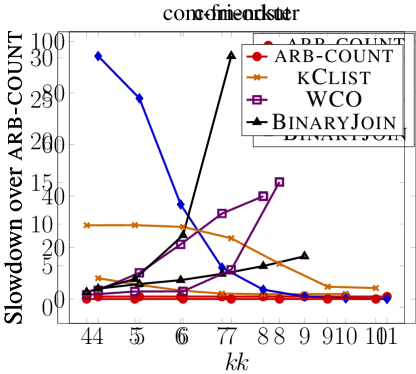
Figure 3: Multiplicative slowdowns of various parallel $k$-clique counting implementations, compared to arb-count, on com-orkut and com-friendster. The best runtimes for each implementation were used, and we have excluded any running time over 5 hours for WCO and BinaryJoin. Note that Pivoter was unable to perform $k$-clique counting on com-friendster due to memory limitations, and as such is not included in this figure.

		$k=3$	$k=4$	$k=5$	$k=6$	$k=7$	$k=8$	$k=9$
com-dblp	arb-peel $T_{60}$	0.14	0.21	0.23∘	1.29∘	18.77	276.69∘	3487.09∘
	arb-peel $T_{1}$	0.27	0.37	1.378	17.99	258.24	3373.05	$>5$ hrs
	kClist $T_{1}$	0.19	0.25	1.10	14.98	221.98	2955.87	$>5$ hrs
	CoreApp $T_{1}$	0.10	0.23	1.09	12.21	244.81	7674.55	$>5$ hrs
com-orkut	arb-peel $T_{60}$	33.15∘	76.91	221.28	721.73	2466.99∘	9062.99∘	$>5$ hrs
	arb-peel $T_{1}$	130.04	184.28	422.20	1032.19	3123.72	$>5$ hrs	$>5$ hrs
	kClist $T_{1}$	87.71	218.94	587.24	2029.43	7414.77	$>5$ hrs	$>5$ hrs
	CoreApp $T_{1}$	113.27	546.13	2460.65	16320.24	$>5$ hrs	$>5$ hrs	$>5$ hrs
com-friendster	arb-peel $T_{60}$	371.52	1747.92	4144.96	6870.06	$>5$ hrs	$>5$ hrs	$>5$ hrs
	arb-peel $T_{1}$	3297.14	11540.73	12932.28	14112.95	$>5$ hrs	$>5$ hrs	$>5$ hrs
	kClist $T_{1}$	2225.70	3216.92	4325.73	6933.32	$>5$ hrs	$>5$ hrs	$>5$ hrs
	CoreApp $T_{1}$	$>5$ hrs	$>5$ hrs	$>5$ hrs	$>5$ hrs	$>5$ hrs	$>5$ hrs	$>5$ hrs
com-lj	arb-peel $T_{60}$	6.46	26.36	324.77	12920.08	$>5$ hrs	$>5$ hrs	$>5$ hrs
	arb-peel $T_{1}$	17.74	70.12	822.10	$>5$ hrs	$>5$ hrs	$>5$ hrs	$>5$ hrs
	kClist $T_{1}$	16.64	42.16	839.13	$>5$ hrs	$>5$ hrs	$>5$ hrs	$>5$ hrs
	CoreApp $T_{1}$	7.20	27.53	1595.04	$>5$ hrs	$>5$ hrs	$>5$ hrs	$>5$ hrs

Table 3: Best runtimes in seconds for our parallel and single-threaded $k$-clique peeling algorithm (arb-peel), as well as the best sequential runtimes from previous work (kClist and CoreApp) [15, 21]. kClist and CoreApp do not have parallel implementations of $k$-clique peeling; they are only serial. The fastest runtimes for each experiment are bolded and in green. All runtimes are from tests in the same computing environment, and include only time spent peeling. For our parallel runtimes, we have chosen the fastest orientations per experiment, while for our serial runtimes, we have fixed the degree orientation. For the parallel runtimes from arb-peel, we have noted the orientation used; ^∘ refers to the Goodrich-Pszona orientation, and no superscript refers to the orientation given by degree ordering.

Environment. We run most of our experiments on a machine with 30 cores (with two-way hyper-threading), with 3.8GHz Intel Xeon Scalable (Cascade Lake) processors and 240 GiB of main memory. For our large compressed graphs, we use a machine with 80 cores (with two-way hyper-threading), with 2.6GHz Intel Xeon E7 (Broadwell E7) processors and 3844 GiB of main memory. We compile our programs with g++ (version 7.3.1) using the -O3 flag. We use OpenMP for our $k$-clique counting runtimes, and we use a lightweight scheduler called Homemade for our $k$-clique peeling runtimes [7]. We terminate any experiment that takes over 5 hours, except for experiments on the large compressed graphs.

Graph Inputs. We test our algorithms on real-world graphs from the Stanford Network Analysis Project (SNAP) [31], CMU’s Lemur project [14], and the WebDataCommons dataset [34]. The details of the graphs are in Table 1, and we show additional statistics in the appendix.

Algorithm Implementations. We test different orientations for our counting and peeling algorithms, including the Goodrich-Pszona and Barenboim-Elkin orientations from Section 3.1, with $\varepsilon=1$. We also test other orientations that do not give work-efficient and polylogarithmic-span bounds, but are fast in practice, including the orientation given by ranking vertices by non-decreasing degree, the orientation given by the $k$-core ordering [33], and the orientation given by the original ordering of vertices in the graph.

Moreover, we compare our algorithms against kClist [15], which contains state-of-the-art parallel and sequential $k$-clique counting algorithms, and sequential $k$-clique peeling implementations. kClist additionally includes a parallel approximate $k$-clique peeling implementation. We include a simple modification to their $k$-clique counting code to support faster $k$-clique counting, where we simply return the number of $k$-cliques instead of iterating over each $k$-clique in the final level of recursion. kClist also offers the option of node or edge parallelism, but only offers a $k$-core ordering to orient the input graphs. Note that kClist does not offer a choice of orientation.

We additionally compare our counting algorithms to Jain and Seshadhri’s Pivoter algorithm [28], Mhedhbi and Salihoglu’s worst-case optimal join algorithm (WCO) [35], Lai et al.’s implementation of a binary join algorithm (BinaryJoin) [30], and Pinar et al.’s ESCAPE algorithm [41]. Note that Pivoter is designed for counting all cliques, and the latter three algorithms are designed for general subgraph counting. Finally, we compare our approximate $k$-clique counting algorithm to Bressan et al.’s MOTIVO algorithm for approximate subgraph counting [11], which is more general. For $k$-clique peeling, we compare to Fang et al.’s CoreApp algorithm [21] and Tsourakakis’s [53] triangle densest subgraph implementation.

5.1 Counting Results

Table 2 shows the best parallel runtimes for $k$-clique counting over the SNAP datasets, from arb-count, kClist, Pivoter, WCO, and BinaryJoin, considering different orientations for arb-count, and considering node versus edge parallelism for arb-count and for kClist. We also show the best sequential runtimes from arb-count. We do not include triangle counting results, because for triangle counting, our $k$-clique counting algorithm becomes precisely Shun and Tangwongsan’s [51] triangle counting algorithm. Furthermore, we performed experiments on ESCAPE by isolating their 4- and 5-clique counting code, but kClist consistently outperforms ESCAPE; thus, we have not included ESCAPE in Table 2. Figure 3 shows the slowdowns of the parallel implementations over arb-count on com-orkut and com-friendster.

We also obtain parallel runtimes for $k=4$ on large compressed graphs, using degree ordering and node parallelism, on a 80-core machine with hyper-threading; note that kClist, Pivoter, WCO, and BinaryJoin cannot handle these graphs. The runtimes are: 5824.76 seconds on ClueWeb with 74 billion edges ($<2$ hours), 12945.25 seconds on Hyperlink2014 with over one hundred billion edges ($<4$ hours), and 161418.89 seconds on Hyperlink2012 with over two hundred billion edges ($<45$ hours). As far as we know, these are the first results for $4$-clique counting for graphs of this scale.

Overall, on 30 cores, arb-count obtains speedups between 1.31–9.88x over kClist, between 1.02–46.83x over WCO, and between 1.20-28.31x over BinaryJoin. Our largest speedups are for large graphs (e.g., com-friendster) and for moderate values of $k$, because we obtain more parallelism relative to the necessary work.

Comparing our parallel runtimes to kClist’s serial runtimes (which were faster than those of WCO and BinaryJoin), we obtain between 2.26–79.20x speedups, and considering only parallel runtimes over 0.7 seconds, we obtain between 16.32–79.20x speedups. By virtue of our orientations, our single-threaded runtimes are often faster than the serial runtimes of the other implementations, with up to 23.17x speedups particularly for large graphs and large values of $k$. Our self-relative parallel speedups are between 13.23–38.99x.

We also compared with Pivoter [28], which is designed for counting all cliques, but can be truncated for fixed $k$. Their algorithm is able to count all cliques for com-dblp and com-orkut in under 5 hours. However, their algorithm is not theoretically-efficient for fixed $k$, taking $O(n\alpha^{2}3^{\alpha/3})$ work, and as such their parallel implementation is up to 196.28x slower compared to parallel arb-count, and their serial implementation is up to 184.76x slower compared to single-threaded arb-count. These slowdowns are particularly prominent for small $k$. Also, Pivoter’s truncated algorithm does not give significant speedups over their full algorithm, and Pivoter requires significant space and runs out of memory for large graphs; it is unable to compute $k$-clique counts at all for $k\geq 4$ on com-friendster.

Of the different orientations, using degree ordering is generally the fastest for small $k$ because it requires little overhead and gives sufficiently low out-degrees. However, for larger $k$, this overhead is less significant compared to the time for counting and other orderings result in faster counting. The cutoff for this switch occurs generally at $k=8$. Note that the Barenboim-Elkin and original orientations are never the fastest orientations. The slowness of the former is because it gives a lower-granularity ordering, since it does not order between vertices deleted in a given round. We found that the self-relative speedups of orienting the graph alone were between 6.69–19.82x across all orientations, the larger of which were found in large graphs. We discuss preprocessing overheads in more detail in the appendix.

Moreover, in both arb-count and kClist, node parallelism is faster on small $k$, while edge parallelism is faster on large $k$. This is because parallelizing the first level of recursion is sufficient for small $k$, and edge parallelism introduces greater parallel overhead. For large $k$, there is more work, which edge parallelism balances better, and the additional parallel overhead is mitigated by the balancing. The cutoff for when edge parallelism is generally faster than node parallelism occurs around $k=8$. We provide more detailed analysis in the appendix.

We also evaluated our approximate counting algorithm on com-orkut and com-friendster, and compared to MOTIVO [11]. We defer a detailed discussion to the appendix. Overall, we obtain significant speedups over exact $k$-clique counting and have low error rates over the exact global counts, with between 5.32–2189.11x speedups over exact counting and between 0.42–5.05% error. We also see 92.71–177.29x speedups over MOTIVO for 4-clique and 5-clique approximate counting on com-orkut.

5.2 Peeling Results

Table 3 shows the best parallel and sequential runtimes for $k$-clique peeling on SNAP datasets for arb-peel, kClist, and CoreApp (kClist and CoreApp only implement sequential algorithms for exact $k$-clique peeling).

Overall, our parallel implementation obtains between 1.01–11.83x speedups over kClist’s serial runtimes. The higher speedups occur in graphs that require proportionally fewer parallel peeling rounds $\rho_{k}$ compared to its size; notably, com-dblp requires few parallel peeling rounds, and we see between 4.78–11.83x speedups over kClist on com-dblp for $k\geq 5$. As such, our parallel speedups are constrained by $\rho_{k}$. Similarly, we obtain up to 53.53x speedup over CoreApp’s serial runtimes. CoreApp outperforms our parallel implementation on triangle peeling for com-dblp, again owing to the proportionally fewer parallel peeling rounds in these cases. arb-peel achieves self-relative parallel speedups between 1.19–13.76x. Our single-threaded runtimes are generally slower than kClist’s and CoreApp’s sequential runtimes owing to the parallel overhead necessary to aggregate $k$-clique counting updates between rounds. In the appendix, we present a further analysis of the distributions of number of vertices peeled per round.

Moreover, the edge density of the approximate $k$-clique densest subgraph found by arb-peel converges towards 1 for $k\geq 3$, and as such, arb-peel is able to efficiently find large subgraphs that approach cliques. In particular, the $k$-clique densest subgraph that arb-peel finds on com-lj contains 386 vertices with an edge density of 0.992. Also, the $k$-clique densest subgraph that arb-peel finds on com-friendster contains 141 vertices with an edge density of 0.993.

We also tested Tsourakakis’s [53] triangle densest subgraph implementation; however, it requires too much memory to run for com-orkut, com-friendster, and com-lj on our machines. It completes $3$-clique peeling on com-dblp in 0.86 seconds, while our parallel arb-peel takes 0.27 seconds.

Finally, we compared our parallel approximate arb-approx-peel to kClist’s parallel approximate algorithm on com-orkut and com-friendster. arb-approx-peel is up to 29.59x faster than kClist for large $k$, and we see between 5.95–80.83% error on the maximum $k$-clique density obtained compared to the density obtained from $k$-clique peeling.

6 Related Work

Theory. A trivial algorithm can compute all $k$-cliques in $O(n^{k})$ work. Using degree-based thresholding enables clique counting in $O(m^{k/2})$ work, which is asymptotically faster for sparse graphs. Chiba and Nishizeki give an algorithm with improved complexity for sparse graphs, in which all $k$-cliques can be found in $O(m\alpha^{k-2})$ work [12], where $\alpha$ is the arboricity of the graph.

For arbitrary graphs, the fastest theoretical algorithm uses matrix multiplication, and counts $3l$ cliques in $O(n^{l\omega})$ time where $\omega$ is the matrix multiplication exponent [37]. The $k$-clique problem is a canonical hard problem in the FPT literature, and is known to be $W[1]$-complete when parametrized by $k$ [19]. We refer the reader to [57], which surveys other theoretical algorithms for this problem.

Recent work by Dhulipala et al. [18] studied $k$-clique counting in the parallel batch-dynamic setting. One of their algorithms calls our arb-count as a subroutine.

Practice. The special case of counting and listing triangles ($k=3$) has received a huge amount of attention over the past two decades (e.g., [55, 54, 51, 39], among many others). Finocchi et al. [23] present parallel $k$-clique counting algorithms for MapReduce. Jain and Seshadri [27] provide algorithms for estimating $k$-clique counts. The state-of-the-art $k$-clique counting and listing algorithm is kClist by Danisch et al. [15], which is based on the Chiba-Nishizeki algorithm, but uses the $k$-core ordering (which is not parallel) to rank vertices. It achieves $O(m\alpha^{k-2})$ work, but does not have polylogarithmic span due to the ordering and only parallelizing one or two levels of recursion. Concurrent with our work, Li et al. [32] present an ordering heuristic for $k$-clique counting based on graph coloring, which they show improves upon kClist in practice. It would be interesting in the future to study their heuristic applied to our algorithm.

Additionally, many algorithms have been designed for finding 4- and 5-vertex subgraphs (e.g., [41, 40, 2, 58, 44]) as well as estimating larger subgraph counts (e.g., [10, 11]), and these algorithms can be used for counting exact or approximate $k$-clique counting as a special case. Worst-case optimal join algorithms from the database literature [1, 38, 35, 30] can also be used for $k$-clique listing and counting as a special case, and would require $O(m^{k/2})$ work.

Very recently, Jain and Seshadri [28] present a sequential and a vertex parallel Pivoter algorithm for counting all cliques in a graph. However, their algorithm cannot be used for $k$-clique listing as they avoid processing all cliques, and requires much more than $O(m\alpha^{k-2})$ work in the worst case.

Low Out-degree Orientations. A canonical technique in the graph algorithms literature on clique counting, listing, and related tasks [20, 28, 41] is the use of a low out-degree orientation. Matula and Beck [33] show that $k$-core gives an $O(\alpha)$ orientation. However, the problem of computing this ordering is $\mathsf{P}$-complete [3], and thus unlikely to have polylogarithmic span. More recent work in the distributed and external-memory literature has shown that such orderings can be efficiently computed in these settings. Barenboim and Elkin give a distributed algorithm that finds an $O(\alpha)$-orientation in $O(\log n)$ rounds [5]. Goodrich and Pszona give a similar algorithm for external-memory [25]. Concurrent with our work, Besta et al. [6] present a parallel algorithm for generating an $O(\alpha)$-orientation in $O(m)$ work and $O(\log^{2}n)$ span, which they use for parallel graph coloring.

Vertex Peeling and $k$-clique Densest Subgraph. An important application of $k$-clique counting is its use as a subroutine in computing generalizations of approximate densest subgraph. In this paper, we study parallel algorithms for $k$-clique densest subgraph, a generalization of the densest subgraph problem introduced by Tsourakakis [53]. Tsourakakis presents a sequential $1/k$-approximation algorithm based on iteratively peeling the vertex with minimum $k$-clique-count, and a parallel $1/(k(1+\epsilon))$-approximation algorithm based on a parallel densest subgraph algorithm of Bahmani et al. [4]. Sun et al. [52] give additional approximation algorithms that converge to produce the exact solution over further iterations; these algorithms are more sophisticated and demonstrate the tradeoff between running times and relative errors. Recently, Fang et al. [21] propose algorithms for finding the largest $(j,\Psi)$-core of a graph, or the largest subgraph such that all vertices have at least $j$ subgraphs $\Psi$ incident on them. They propose an algorithm for $\Psi$ being a $k$-clique that peels vertices with larger clique counts first and show that their algorithm gives a $1/k$-approximation to the $k$-clique densest subgraph.

7 Conclusion

We presented new work-efficient parallel algorithms for $k$-clique counting and peeling with low span. We showed that our implementations achieve good parallel speedups and significantly outperform state-of-the-art. A direction for future work is designing work-efficient parallel algorithms for the more general $(r,s)$-nucleus decomposition problem [48].

A Examples

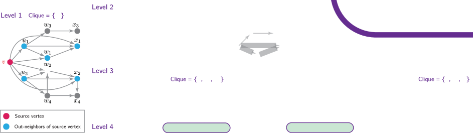
Figure 4: An example of our $k$-clique counting algorithm for $k=4$.

Figure 4 shows an example of our $k$-clique counting algorithm, arb-count, for $k=4$. First, the graph is directed as shown in Level 1. The algorithm then iterates over all vertices in parallel, but for simplicity we only show a single process starting from vertex $v$. Importantly, the algorithm must iterate over all vertices, since there are 4-cliques that are not found by starting at $v$. For instance, $\{w_{2},x_{2},w_{4},x_{4}\}$ is a 4-clique that is found by running this process starting from $w_{4}$.

We call $v$ the source vertex for its process in Level 1, and note that $v$ is added to the growing clique set. Each directed out-neighbor of $v$, in blue, spawns a new child task where the out-neighbor is added to the growing clique set and is denoted as the new source vertex, as shown in Level 2.

In Level 2, we take each source vertex, in red, and intersect its out-neighbors, in blue, with its parent task’s out-neighbors, contained within the dashed blue circle. Note that all vertices $x_{i}$ have no out-neighbors, so these tasks terminate here. For simplicity, we have removed the parent task’s source vertex $v$, because no level 2 source vertices may have $v$ as an out-neighbor by virtue of our orientation, and we have also removed any vertices disconnected from the source vertex. Now, each vertex in the aforementioned intersection (i.e., each blue vertex in the dashed blue circle) spawns a new child task, where it is added to the growing clique set and becomes the new source vertex, as shown in Level 3. The dashed blue circle shrinks to contain only the out-neighbors in the intersection from Level 2.

We repeat this process for a final level, intersecting the out-neighbors, in blue, of the source vertices, in red, with the intersection from the previous level, in the dashed blue circle. Each vertex remaining in the intersection spawns a new child task. The child tasks remaining in Level 4 represent our 4-cliques. For example, the 4-clique $\{v,u_{2},w_{2},x_{2}\}$ is obtained by intersecting $w_{2}$’s out-neighbors $\{x_{2},x_{4}\}$ and $u_{2}$’s out-neighbors $\{w_{2},w_{4},x_{2}\}$, which gives $\{x_{2}\}$ and adding the source vertices on the path to this task, $\{v,u_{2},w_{2}\}$. Note that the arrows between the levels in this figure represent the dependency graph for the 4-clique counting computation; the spawned child tasks are all safe to run in parallel.

B Proofs

We present here proofs for the complexity bounds for our low out-degree orientation algorithms, approximate $k$-clique counting algorithm using colorful sparsification, $k$-clique vertex peeling algorithm, and approximate $k$-clique vertex peeling algorithm. Additionally, we prove the variance of our estimator in our approximate $k$-clique counting algorithm, and we prove that the problem of obtaining the $k$-clique cores given by the $k$-clique vertex peeling process is $\mathsf{P}$-complete.

B.1 Low Out-degree Orientation (Ranking)

1:procedure Orient($G=(V,E)$, $\epsilon$)

2:     $n\leftarrow|V|,L\leftarrow[]$

3:     while $G$ is not empty do

4:         $S\leftarrow\epsilon n/(2+\epsilon)$ vertices of lowest induced degree

5:         Append $S$ to $L$

6:         Remove vertices in $S$ from $G$      

7:     return $L$

Algorithm 3 Goodrich-Pszona Orientation Algorithm

1:procedure Orient($G=(V,E)$, $\epsilon$, $\alpha$)

2:     $n\leftarrow|V|,L\leftarrow[]$

3:     while $G$ is not empty do

4:         $S\leftarrow\{v\in V\ |\$ $v$’s induced degree less than $(2+\epsilon)\alpha\}$

5:         Append $S$ to $L$

6:         Remove vertices in $S$ from $G$      

7:     return $L$

Algorithm 4 Barenboim-Elkin Orientation Algorithm

Algorithms 3 and 4 shows pseudocode for the Goodrich-Pszona algorithm and the Barenboim-Elkin algorithm respectively. We present here the bounds for our parallelization of these algorithms, which are described in Section 3.1.

See 3.1

• The bounds on out-degree follow from the discussion in Section 3.1. Also, as discussed in Section 3.1, both algorithms run in $O(\log n)$ rounds, because each round removes a constant fraction of the vertices. It remains to prove the work and span bounds for both algorithms. Note that for both algorithms, we maintain the induced degrees of all vertices in an array.

For the Goodrich-Pszona algorithm, we can filter out the vertices with degree less than the $c$’th smallest degree vertex for $c=\epsilon n/(2+\epsilon)$ using parallel integer sort, which runs in $O(n^{\prime})$ work whp, $O(\log n)$ span whp, and $O(n^{\prime})$ space, where $n^{\prime}$ is the number of remaining vertices [42]. For the Barenboim-Elkin algorithm, we use a parallel filter, which takes linear work, $O(\log n)$ span, and linear space. Overall, the total work to obtain vertices to process in each round for both algorithms is $O(n)$ (whp for Goodrich-Pszona), because each round removes a constant fraction of vertices.

We can update the degrees of the remaining vertices after removing the peeled vertices by mapping over all edges incident to these vertices, and applying an atomic add instruction to decrement the degree of each neighbor. Each edge is processed exactly once in each direction, when its corresponding endpoints are peeled, and each vertex is peeled exactly once, so the total work is $O(m)$. Since each peeling round can be implemented in $O(\log n)$ span, and there are $O(\log n)$ such rounds, the span of both algorithms is $O(\log^{2}n)$.

Finally, computing an estimate of the arboricity using the parallel densest-subgraph algorithm from [17] can be done in $O(m)$ work, $O(\log^{2}n)$ span, and $O(m)$ space, which does not asymptotically increase the cost of running the Barenboim-Elkin algorithm.         

B.2 Sampling

We present here the proof for the variance of our estimator in approximate $k$-clique counting through colorful sparsification, which is described in Section 3.3.

Theorem B.1

Let $X$ be the true $k$-clique count in $G$, $C$ be the $k$-clique count in $G^{\prime}$, $p=1/c$, and $Y=C/p^{k-1}$. Then $\mathbb{E}[Y]=X$ and $\mathbb{V}ar[Y]=p^{-2(k-1)}(X(p^{k-1}-p^{2(k-1)})+\sum_{z=2}^{k-1}s_{z}(p^{2(k-1)-z+1}-p^{2(k-1)}))$, where $s_{z}$ is the number of pairs of $k$-cliques that share $z$ vertices.

• Let $C_{i}$ be an indicator variable denoting whether the $i$’th $k$-clique in $G$ is preserved in $G^{\prime}$. For a $k$-clique to be preserved, all $k$ vertices in the clique must have the same color. This happens with probability $p^{k-1}$ since after fixing the color of one vertex $v$ in the clique, the remaining $k-1$ vertices must have the same color as $v$. Each vertex picks a color independently and uniformly at random, and so the probability of a vertex choosing the same color as $v$ is $p$. The number of $k$-cliques in $G^{\prime}$ is equal to $C=\sum_{i}{C_{i}}$. Therefore $\mathbb{E}[C]=\sum_{i}\mathbb{E}[C_{i}]=Xp^{k-1}$. We have that $\mathbb{E}[Y]=\mathbb{E}[C/p^{k-1}]=(1/p^{k-1})\mathbb{E}[C]=(1/p^{k-1})Xp^{k-1}=X$.

  The variance of $Y$ is $\mathbb{V}ar[Y]=\mathbb{V}ar[C/p^{k-1}]=\mathbb{V}ar[C]/p^{2(k-1)}=\mathbb{V}ar[\sum_{i}C_{i}]/p^{2(k-1)}$. By definition $\mathbb{V}ar[\sum_{i}C_{i}]=\sum_{i}(\mathbb{E}[C_{i}]-\mathbb{E}[C_{i}]^{2})+\sum_{i\neq j}\mathbb{C}ov[C_{i},C_{j}]$. The first term is equal to $X(p^{k-1}-p^{2(k-1)})$. To compute the second term, note that $\mathbb{C}ov[C_{i},C_{j}]=\mathbb{E}[C_{i}C_{j}]-\mathbb{E}[C_{i}]\mathbb{E}[C_{j}]$ depends on the number of vertices that cliques $i$ and $j$ share. Their covariance is $0$ if they share no vertices. Their covariance is also $0$ if they share one vertex since the event that the remaining vertices of each clique have the same color as the shared vertex is independent between the two cliques. Let $s_{z}$ denote the number of pairs of cliques that share $z>1$ vertices. For pairs of cliques sharing $z$ vertices, we have $\mathbb{E}[C_{i}C_{j}]=p^{2(k-1)-z+1}$. This is because after fixing the color of one of the shared vertices, there are $2(k-1)-z+1$ remaining vertices in the pair of cliques to color, and the probability that they all match the fixed color is $p^{2(k-1)-z+1}$. Therefore $\mathbb{C}ov[C_{i},C_{j}]=\mathbb{E}[C_{i}C_{j}]-\mathbb{E}[C_{i}]\mathbb{E}[C_{j}]=p^{2(k-1)-z+1}-p^{2(k-1)}$. In total, we have $\mathbb{V}ar[Y]=p^{-2(k-1)}(X(p^{k-1}-p^{2(k-1)})+\sum_{z=2}^{k-1}s_{z}(p^{2(k-1)-z+1}-p^{2(k-1)}))$.         

We also give the proof for the work and span of approximate $k$-clique counting through colorful sparsification.

See 3.3

• Theorem B.1 states that our algorithm produces an unbiased estimate of the global count. We now analyze the work and span of the algorithm. Choosing colors for the vertices can be done in $O(n)$ work and $O(1)$ span. Creating a subgraph containing edges with endpoints having the same color can be done using prefix sum and filtering in $O(m)$ work and $O(\log m)$ span. Each edge is kept with probability $p$ as the two endpoints will have matching colors with this probability. Therefore, our subgraph has $pm$ edges in expectation. The arboricity of our subgraph is upper bounded by the arboricity of our original graph, $\alpha$, and so including the work of running our $k$-clique counting algorithm on the subgraph, the sampling algorithm takes $O(pm\alpha^{k-2}+m)$ work and $O(k\log n+\log^{2}n)$ span whp.         

B.3 Vertex Peeling

We present here the proof that arb-peel correctly generates a subgraph with the same approximation guarantees of Tsourakakis’ sequential $k$-clique densest subgraph algorithm [53], as well as the following bounds on the complexity of arb-peel.

See 4.1

This proof uses the Nash-Williams theorem [36], which states that a graph $G$ has arboricity $\alpha$ if and only if for every $U\subseteq V$, $|G[U]|\leq\alpha(|U|-1)$. Here, $G[U]$ is the subgraph of $G$ induced by the vertices in $U$, and $|G[U]|$ is the number of edges in $G[U]$.

First, we provide a proof on the correctness of our $k$-clique peeling algorithm. Tsourakakis [53] proves that the sequential $k$-clique densest subgraph algorithm that peels vertices one by one in increasing order of $k$-clique count attains a $1/k$-approximation to the $k$-clique densest subgraph problem. We note that among vertices within the same $k$-clique core, the order in which these vertices are peeled does not affect the approximation; this follows directly from Tsourakakis’s sequential algorithm, in which in any given round, any vertex with the same minimum $k$-clique count may be peeled. Additionally, given a set of vertices with the same minimum $k$-clique count in any given round, peeling a vertex from this set does not change the $k$-clique core number of any other vertex in this set by definition.

As such, in order to show the correctness of arb-peel, it suffices to show that first, arb-peel peels vertices in the same order as given by Tsourakakis’s sequential algorithm, except for vertices in the same $k$-clique core which may be peeled in any order among each other, and second, arb-peel correctly updates the $k$-clique counts after peeling these vertices. The first claim follows from the structure of arb-peel, because arb-peel peels all vertices with the same minimum $k$-clique count in each round, which may be serialized to any order. The second claim follows from the correctness of arb-count in Section 3. arb-peel first obtains for each peeled vertex $v$ all undirected neighbors $N(v)$, and then uses the subroutine from arb-count to obtain $k$-cliques originating from $v$. This is equivalent to first obtaining the induced subgraph on $N(v)$, and then performing arb-count to obtain $(k-1)$-cliques on the induced subgraph; thus, this gives all $k$-cliques containing $v$. The additional filtering of already peeled vertices ensures that previously found $k$-cliques are not recounted, and filtering other vertices peeled simultaneously based on a total order ensures that $k$-cliques involving these vertices are not recounted. Thus, arb-peel gives a $1/k$-approximation to the $k$-clique densest subgraph problem.

The proof of the complexity is similar in spirit to that of Theorem 3.2, but there are some subtle and important differences. First, unlike in our $k$-clique counting algorithm (Algorithm 1), our peeling algorithm does not have the luxury of only finding $k$-cliques directed out of a peeled vertex $v$. Instead, it must find all $k$-cliques that $v$ participates in and decrement these counts. Arguing that this does not cost a prohibitive amount of work is the main challenge of the proof. Importantly, our peeling algorithm calls the recursive subroutine rec-count-cliques-v of our $k$-clique counting algorithm directly, on a different input than used in the full $k$-clique counting algorithm, and so the analysis of the work and span differs from the analysis given in Section 3.2.

We first account for the work and span of extracting and updating the bucketing structure. The overall work of inserting vertices into the structure is $O(n)$. Each vertex has its bucket decremented at most once per $k$-clique, and since there are at most $O(m\alpha^{k-2})$ $k$-cliques, this is also the total cost for updating buckets of vertices. Lastly, removing the minimum bucket can be done in $O(\log n)$ amortized expected work and $O(\log n)$ span whp, which costs a total of $O(\rho_{k}(G)\log n)$ amortized expected work, and $O(\rho_{k}(G)\log n)$ span whp.

Next, to bound the cost of finding all $k$-cliques incident to a peeled vertex $v$, we rely on the Nash-Williams theorem, which provides a bound on the size of induced subgraphs in a graph with arboricity $\alpha$. Notably, in the first level of recursion when rec-count-cliques-v is called from the Update subroutine, the intersect operations performed essentially compute the induced subgraph on the neighbors of each peeled vertex $v$; this is because during this call, we intersect the directed neighbors of each vertex in $N_{G}(v)$ (that has not been previously peeled) with $N_{G}(v)$ itself, producing a pruned version of the induced subgraph of $N_{G}(v)$ on $G$. We have that for each $v\in V$, the induced subgraph on its neighbors has size $|G[N(v)]|\leq\alpha(|N(v)|-1)=\alpha(d(v)-1)$. Assuming for now that we can construct the induced subgraph on all vertex neighborhoods in work linear in their size, summed over all vertices, the overall cost is just

(B.1) $$\sum_{v\in V}|G[N(v)]|\leq\alpha\sum_{v\in V}(d(v)-1)=O(m\alpha)$$

How do we build these subgraphs in the required work and span? Our approach is to do so using an argument similar to the elegant proof technique proposed in Chiba-Nishizeki’s original $k$-clique listing algorithm [12]. Because the first call to rec-count-cliques-v takes each vertex $u\in N_{G}(v)$ and intersects the directed neighbors $N_{DG}(u)$ with $N_{G}(v)$, we use $O(\min(d(u),d(v)))$ work to build the induced subgraph on $v$’s neighborhood. Observe that each edge in the graph is processed by an intersection in this way exactly once in each direction, when each endpoint is peeled. By Lemma 2 of [12], we know that $\sum_{e=(u,v)\in E}\min(d(u),d(v))=O(m\alpha)$ and therefore the overall work of performing all intersections is bounded by $O(m\alpha)$, and the per-vertex induced subgraphs can therefore also be built in the same bound. The span for this step is $O(\log n)$ whp using parallel hash tables [24].

Lastly, we account for the remaining cost of performing $k$-clique counting within each round. We now recursively call rec-count-cliques-v $k-1$ times in total, as $\ell$ ranges from $1$ to $k-1$, but the final recursive call returns the size of $I$ immediately, and we have already discussed the work of the first call to rec-counts-v. Considering the remaining $k-3$ recursive steps with non-trivial work, we have $O(m^{\prime}\alpha^{k-3})$ work and $O(k\log n)$ span where $m^{\prime}$ is the size of the vertex’s induced neighborhood. Considering the work first, summed over all vertices’ induced neighborhoods, the total work is

$$\sum_{v\in V}\operatorname{O}\left(|G[N(v)]|\alpha^{k-3}\right)=O(m\alpha^{k-2})$$

which follows from Equation B.1. The span follows, since adding in the span of the first recursive call, we have $O(k\log n)$ span to update $k$-clique counts per peeled vertex, and there are $\rho_{k}(G)$ rounds by definition.         

B.4 Parallel Complexity of Vertex Peeling

The $k$-clique vertex peeling algorithm exactly computes for all $c$ the $k$-clique $c$-cores of the graph. The $k$-clique $c$-core of a graph $G$ is defined as the maximal subgraph such that every vertex is contained within at least $c$ $k$-cliques. This is a generalization of the classic $c$-core problem, which is the maximal subgraph such that each vertex has degree at least $c$. The $c$-core problem is well known to be $\mathsf{P}$-complete for $c\geq 3$ [3]. We present here the proof that computing $k$-clique $c$-cores is $\mathsf{P}$-complete for $c>2$. We first observe that since the number of $k$-cliques incident to each vertex can be efficiently computed in $\mathsf{NC}$ by Theorem 3.2, the problem of computing $k$-clique $1$-cores is in $\mathsf{NC}$ for constant $k$.

$k$-clique $\bm{c}$-cores when $\bm{c>2}$. Next, we study the parallel complexity of computing $k$-clique $c$-cores for $c>2$. We will show that there is an $\mathsf{NC}$ reduction from the problem of deciding whether the $c$-core is non-empty, to the problem of deciding whether the $k$-clique $c$-core is non-empty. We first discuss the reduction at a high level. The input is a graph and some value $c$, and the problem is to decide whether the $c$-core is non-empty. The idea is to map the original peeling process to compute the $c$-core to a peeling process to compute the $k$-clique $c$-core. Figure 5 shows the reduction for $k=3,c=7$, and marks the initial $k$-clique degrees of each vertex in red.

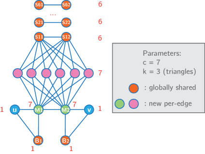
Figure 5: Gadget used for the reduction for computing 3-clique $c$-cores for an original edge $(u,v)$, shown for $c=7$. The red numbers next to each vertex show the vertex’s $3$-clique degree, or the number of $3$-cliques incident per vertex before peeling (as a contribution of the gadget for this $(u,v)$ edge). The pink gadget vertices and green middle vertices are distinct per edge in the reduction. The orange special vertices and base vertices are created only once and globally shared. The gadget shown here gives each of the green middle vertices, $M_{1}$ and $M_{2}$, a $3$-clique degree of $c=7$, with one of the incident triangles being formed by an original vertex endpoint (either $u$ or $v$), and the remaining being formed with the pink gadget vertices. Each of the pink gadget vertices forms one triangle with the green middle vertices, and the remaining $c-1$ triangles with $c-1$ pairs of special (globally shared) vertices, $S_{ij}$. Modifying this construction for different values of $c$ is done by creating $c-1$ pink gadget vertices and $c-1$ special-vertex pairs. To generalize to $k>3$ we make the base vertices $B_{1}$ and $B_{2}$ each a $(k-2)$-clique which are fully connected to $u$ and one of the green middle vertices to form $k$-cliques. Similarly, each pink gadget vertex becomes a $(k-2)$-clique to form $c-1$ $k$-cliques with the green middle vertices.

The reduction works as follows. We break up each edge $(u,v)$ in the graph into four vertices connected in a path with the left-most and right-most vertices corresponding to the original vertices $u$ and $v$. The middle vertices are $M_{1}$ and $M_{2}$ (shown in green in Figure 5). We create gadgets to increase each of the two middle vertices’ $k$-clique degrees to $c$. The gadgets are constructed so that if either of the original vertices has its $k$-clique degree go below $c$ and is thus not in the $k$-clique $c$-core, then the path corresponding to this edge will unravel, and the other original vertex will have its $k$-clique degree decremented by one, exactly as in the $c$-core peeling process.

The reduction constructs $c-1$ $k$-cliques between the two middle vertices in the path, and a set of new gadget vertices for this edge (shown in pink in Figure 5). It also constructs one $k$-clique between each original edge endpoint, its neighboring middle vertex, and a specially designated set of base vertices, which are globally shared. The last part of the construction ensures that the gadget vertices have large enough $k$-clique degrees by creating $c-1$ $k$-cliques between them and a set of special vertices, $S_{i}$’s, which are globally shared.

To argue that this reduction is correct, it suffices to show that the $k$-clique $c$-core is non-empty if and only if the $c$-core of the original graph is non-empty. We only argue the reverse direction, since the proof for the forward direction is almost identical. Suppose the input graph has a non-empty $c$-core, $C$. Then, observe that all of the original vertices corresponding to $C$ in the reduction graph have $k$-clique degree at least $c$. Furthermore, since all of the middle vertices that are added for original edges in the $c$-core initially have $k$-clique degree exactly $c$, the gadget vertices corresponding to these edges have $k$-clique degree exactly $c$. It remains to argue that the special vertices and the base vertices have sufficient $k$-clique degree. Observe that the special vertices connected to all gadget vertices for the edges form $k$-cliques with all gadget vertices, and thus have $k$-clique degree $(c-1)|E(G[C])|$, where $E(G[C])$ is the set of edges in the induced subgraph on $C$. Since a $c$-core on $|C|$ vertices must have at least $c|C|$ edges, $(c-1)|E(G[C])|\geq(c-1)c|C|>c$. Similarly for the base vertices, they form a single $k$-clique for each edge in the $c$-core, and so the base vertices have $k$-clique degree $c|C|$. Thus, the subgraph corresponding to the original vertices, middle vertices, and gadget vertices for these edges, and the special and base vertices all have sufficient $k$-clique degree to form a non-empty $k$-clique $c$-core.

By the discussion above, we have shown that computing $k$-clique $c$-cores is $\mathsf{P}$-complete for $c>2$, a strengthening of the original $\mathsf{P}$-completeness result of Anderson and Mayr [3].

An interesting question is to understand the parallel complexity of computing $k$-clique $2$-cores for any constant $k$. For $k=2$, Anderson and Mayr observed that this problem is in $\mathsf{NC}$. We leave it for future work to determine whether a similar algorithm can find the $k$-clique $2$-cores in $\mathsf{NC}$ for $k>2$.

B.5 Approximate Vertex Peeling

We now present the proof for the work and span of our approximate $k$-clique peeling algorithm, arb-approx-peel, from Section 4.2.

See 4.2

• The correctness and approximation guarantees of this algorithm follows from [53]. The work bound follows similarly to the proof of Theorem 4.1. Also, filtering the remaining vertices in each round can be done in $O(n)$ total work, since a constant fraction of vertices are peeled in each round. The span bound follows because there are $O(\log n)$ rounds in total, and since each round runs in $O(k\log n)$ span, again using the same argument given in Theorem 4.1.         

	$k=4$	$k=5$	$k=6$	$k=7$	$k=8$	$k=9$	$k=10$	$k=11$
com-dblp	16,713,192	262,663,639	$4.222\times 10^{9}$	$6.091\times 10^{10}$	$7.772\times 10^{11}$	$8.813\times 10^{12}$	$8.956\times 10^{13}$	—
com-orkut	$3.222\times 10^{9}$	$1.577\times 10^{10}$	$7.525\times 10^{10}$	$3.540\times 10^{11}$	$1.633\times 10^{12}$	$7.248\times 10^{12}$	$3.029\times 10^{13}$	$1.171\times 10^{14}$
com-friendster	$8.964\times 10^{9}$	$2.171\times 10^{10}$	$5.993\times 10^{10}$	$2.969\times 10^{11}$	$3.120\times 10^{12}$	$4.003\times 10^{13}$	$4.871\times 10^{14}$	—
com-lj	$5.217\times 10^{9}$	$2.464\times 10^{11}$	$1.099\times 10^{13}$	$4.490\times 10^{14}$	—	—	—	—
ClueWeb	$2.968\times 10^{14}$	—	—	—	—	—	—	—
Hyperlink2014	$7.500\times 10^{14}$	—	—	—	—	—	—	—
Hyperlink2012	$7.306\times 10^{15}$	—	—	—	—	—	—	—

Table 4: Total $k$-clique counts for our input graphs. Note that we do not have statistics for certain graphs for large values of $k$, because algorithm did not terminate in under 5 hours; these entries are represented by a dash.

C Additional Experiments and Data

This section presents additional experimental data from our evaluation.

C.1 Counting Results

Figure 4 shows the $k$-clique counts that we obtained from our algorithms. Figure 6 shows the frequencies of the 4-clique counts per vertex, as obtained using arb-count, on the large ClueWeb and Hyperlink2014 graphs. We see that the number of vertices decreases roughly exponentially as a function of the 4-clique count.

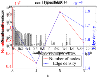
Figure 6: The frequencies of 4-clique counts per vertex, obtained using arb-count, on the large graphs ClueWeb and Hyperlink2014. Note that the frequencies is plotted on a log-scale.

Figure 7 shows the preprocessing overheads and $k$-clique counting times for com-orkut using different orientations and node parallelism. The Goodrich-Pszona orientation is 2.86x slower than the orientation using degree ordering, but this overhead is not significant for large $k$ and the Goodrich-Pszona orientation gives the fastest counting times for large $k$. We found that the self-relative speedups of orienting the graph alone were between 6.69–19.82x across all orientations, the larger of which were found in the larger graphs.

Figure 7: Parallel runtimes for $k$-clique counting (arb-count) on com-orkut for different orientations, using node parallelism. All times are scaled by the fastest parallel time (indicated in parentheses). The first set of bars show the preprocessing overhead of the different orientations. The remaining sets of bars show the performance including both preprocessing and counting.

In both arb-count and kClist, node parallelism is faster on small $k$, while edge parallelism is faster on large $k$, due to the greater work required on large $k$ and the additional parallelism available in edge parallelism to take advantage of this work. The cutoff for when edge parallelism is generally faster than node parallelism occurs around $k=8$. Figure 8 shows this behavior in arb-count’s $k$-clique counting runtimes on com-orkut, where for $k\geq 9$ edge parallelism becomes faster than node parallelism.

Figure 9 show the runtimes for our approximate counting algorithm on com-orkut and com-friendster. We see that there is an inflection point where after enough sparsification, obtaining $k$-clique counts for large $k$ is faster than for small $k$; this is because we cut off the recursion when there are not enough vertices to complete a $k$-clique. We compute our error rates as $|\text{exact}-\allowbreak\text{approximate}|/\text{exact}$. For $p=0.5$ on both com-orkut and com-friendster across all $k$, we see between 2.42–87.56x speedups over exact counting (considering the best $k$-clique counting runtimes) and between 0.39–1.85% error. Our error rates degrade for higher $k$ and lower $p$, but even for $p$ as low as $0.125$, we obtain between 5.32–2189.11x speedups over exact counting and between 0.42–5.05% error.

We compare our approximate counting algorithms to approximate $k$-clique counting using MOTIVO [11]. We ran both the naive sampling and adaptive graphlet sampling (AGS) options in MOTIVO. However, MOTIVO is unable to run on com-friendster because it runs out of memory. Moreover, in order to achieve a 6% error rate, MOTIVO takes between 92.71–177.29x the time that our algorithm takes for 4-clique and 5-clique approximate counting on com-orkut. MOTIVO takes 168.84 seconds to approximate 6-clique counts with 31.55% error, while our algorithm takes 0.49 seconds to approximate 6-clique counts with under 6% error. However, unlike our algorithm, MOTIVO can estimate non-clique subgraph counts.

C.2 Peeling Results

Figure 5 shows the peeling rounds, $k$-clique core sizes, and approximate maximum $k$-clique densities that we obtained from our algorithms.

Figure 10 shows the frequencies of the different numbers of vertices peeled in each parallel round for com-orkut, for $4\leq k\leq 6$. A significant number of rounds contain fewer than 50 vertices peeled, and by the time we reach the tail of the histogram, there are very few parallel rounds with a large number of vertices peeled.

Figures 11 and 12 show the parallel runtimes of arb-approx-peel and of kClist’s approximate peeling algorithm on com-orkut and com-friendster, respectively. Note that while kClist only provides a sequential implementation for exact $k$-clique peeling, kClist provides a parallel implementation for approximate $k$-clique peeling. We found there was not a significant difference in performance across different values of $\epsilon$ for both implementations. arb-approx-peel is up to 29.59x faster than kClist for large $k$. However, arb-approx-peel was slower on com-friendster for small $k$ since kClist uses a serial heap to recompute vertices to be peeled; this is more amenable over rounds containing fewer vertices, while our implementation incurs additional overhead to recompute peeled vertices in parallel, which is mitigated over larger $k$. In terms of percentage error in the maximum $k$-clique density obtained compared to the density obtained from $k$-clique peeling, we see between 48.58–77.88% error on com-orkut and 5.95–80.83% error on com-friendster.

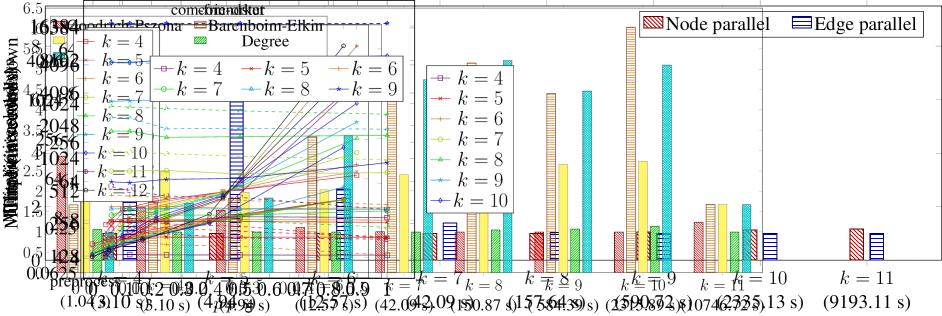
Figure 8: Parallel runtimes for $k$-clique counting (arb-count) on com-orkut, considering node parallelism and edge parallelism, and fixing the orientation given by degree ordering. All times are scaled by the fastest parallel runtime, which are given in the parentheses.

Figure 9: Parallel runtimes for approximate $k$-clique counting (arb-count) on com-orkut and com-friendster, varying over $p=1/c$ where $c$ is the number of colors used. The runtimes were obtained using the orientation given by degree ordering and node parallelism. The $y$-axis is in log-scale.

		$k=3$	$k=4$	$k=5$	$k=6$	$k=7$	$k=8$	$k=9$
	$\rho_{k}$	5,626	11,669	17,720	22,091	23,988	23,095	21,538
	Max density ($k$-clique peeling)	10,100	297,096	5,598,323	75,372,336	782,071,056	$6.183\times 10^{9}$	$4.080\times 10^{10}$
	$\rho_{k}$	483	441	343	240	166	127	103
com-dblp	$k$-clique core	6,328	234,136	6,438,740	140,364,532	$2.527\times 10^{9}$	$3.862\times 10^{10}$	$5.117\times 10^{11}$
	Max density ($k$-clique peeling)	6,328	234,136	6,438,740	140,364,532	$2.527\times 10^{9}$	$3.862\times 10^{10}$	$5.117\times 10^{11}$
	$\rho_{k}$	36,752	94,931	160,577	210,966	236,623	241,330	—
com-orkut	$k$-clique core	7,117	117,182	2,115,900	29,272,988	312,629,724	$2.741\times 10^{9}$	—
	Max density ($k$-clique peeling)	18,547	340,997	4,882,477	73,696,814	883,634,847	$8.332\times 10^{9}$	—
	$\rho_{k}$	57,090	140,705	249,605	339,347	—	—	—
com-friendster	$k$-clique core	8,255	349,377	11,001,375	274,901,025	—	—	—
	Max density ($k$-clique peeling)	9,521	428,928	12,762,919	363,676,399	—	—	—
	$\rho_{k}$	13,899	29,514	42,994	50,159	—	—	—
com-lj	$k$-clique core	64,478	7,660,975	679,343,769	$4.796\times 10^{10}$	—	—	—
	Max density ($k$-clique peeling)	72,255	9,031,923	839,813,448	$6.199\times 10^{10}$	—	—	—

Table 5: Relevant $k$-clique peeling statistics for the SNAP graphs that we experimented on. We do not have statistics for certain graphs for large values of $k$, because the corresponding $k$-clique peeling algorithms did not terminate in under 5 hours; these entries are represented by a dash.

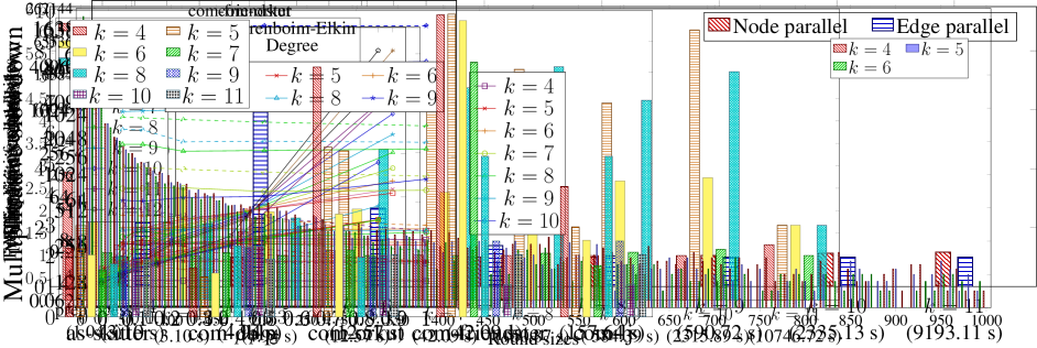
Figure 10: Frequencies of the number of vertices peeled in a parallel round using arb-peel, for $k$-clique peeling on com-orkut ($4\leq k\leq 6$). Rounds with more than 1000 vertices peeled have been truncated; these truncated round frequencies are very low, most often consisting of 0 rounds. The frequencies are given in log-scale.

Figure 11: Parallel runtimes on com-orkut for approximate $k$-clique peeling using arb-approx-peel (solid lines) and kClist (dashed lines). These runtimes were obtained by varying over $\epsilon$, giving a $1/(k(1+\epsilon))$-approximation of the $k$-clique densest subgraph. These runtimes were obtained using the orientation given by degree ordering, and the runtimes are given in log-scale. Moreover, we cut off kClist’s runtimes at 5 hours, which occurred for $k=10$ over all $\varepsilon$.

Figure 12: Parallel runtimes on com-friendster for approximate $k$-clique peeling using arb-approx-peel (solid lines) and kClist (dashed lines). These runtimes were obtained by varying over $\epsilon$, giving a $1/(k(1+\epsilon))$-approximation of the $k$-clique densest subgraph. These runtimes were obtained using the orientation given by degree ordering, and the runtimes are given in log-scale. Moreover, we cut off kClist’s runtimes at 5 hours, which occurred for $k=9$ over all $\varepsilon$.

References

- [1] C. R. Aberger, A. Lamb, S. Tu, A. Nötzli, K. Olukotun, and C. Ré. EmptyHeaded: A relational engine for graph processing. ACM Trans. Database Syst., 42(4), 2017.
- [2] N. K. Ahmed, J. Neville, R. A. Rossi, N. G. Duffield, and T. L. Willke. Graphlet decomposition: framework, algorithms, and applications. Knowl. Inf. Syst., 50(3), 2017.
- [3] R. Anderson and E. W. Mayr. A -complete problem and approximations to it. Technical report, 1984.
- [4] B. Bahmani, R. Kumar, and S. Vassilvitskii. Densest subgraph in streaming and MapReduce. Proc. VLDB Endow., 5(5), Jan. 2012.
- [5] L. Barenboim and M. Elkin. Sublogarithmic distributed MIS algorithm for sparse graphs using Nash-Williams decomposition. Distributed Computing, 22(5), 2010.
- [6] M. Besta, A. Carigiet, K. Janda, Z. Vonarburg-Shmaria, L. Gianinazzi, and T. Hoefler. High-performance parallel graph coloring with strong guarantees on work, depth, and quality. In ACM/IEEE International Conference for High Performance Computing, Networking, Storage and Analysis, 2020.
- [7] G. E. Blelloch, D. Anderson, and L. Dhulipala. Brief announcement: ParlayLib – a toolkit for parallel algorithms on shared-memory multicore machines. In ACM Symposium on Parallelism in Algorithms and Architectures, 2020.
- [8] R. D. Blumofe and C. E. Leiserson. Space-efficient scheduling of multithreaded computations. SIAM J. Comput., 27(1), 1998.
- [9] R. P. Brent. The parallel evaluation of general arithmetic expressions. J. ACM, 21(2), Apr. 1974.
- [10] M. Bressan, F. Chierichetti, R. Kumar, S. Leucci, and A. Panconesi. Motif counting beyond five nodes. ACM Trans. Knowl. Discov. Data, 12(4), 2018.
- [11] M. Bressan, S. Leucci, and A. Panconesi. Motivo: Fast motif counting via succinct color coding and adaptive sampling. Proc. VLDB Endow., 12(11), July 2019.
- [12] N. Chiba and T. Nishizeki. Arboricity and subgraph listing algorithms. SIAM J. Comput., 14(1), Feb. 1985.
- [13] T. H. Cormen, C. E. Leiserson, R. L. Rivest, and C. Stein. Introduction to Algorithms (3. ed.). MIT Press, 2009.
- [14] B. Croft and J. Callan. The Lemur project. https://www.lemurproject.org/, 2016.
- [15] M. Danisch, O. Balalau, and M. Sozio. Listing -cliques in sparse real-world graphs*. In International Conference on World Wide Web, 2018.
- [16] L. Dhulipala, G. Blelloch, and J. Shun. Julienne: A framework for parallel graph algorithms using work-efficient bucketing. In ACM Symposium on Parallelism in Algorithms and Architectures, 2017.
- [17] L. Dhulipala, G. E. Blelloch, and J. Shun. Theoretically efficient parallel graph algorithms can be fast and scalable. In ACM Symposium on Parallelism in Algorithms and Architectures, 2018.
- [18] L. Dhulipala, Q. C. Liu, J. Shun, and S. Yu. Parallel batch-dynamic -clique counting. In SIAM Symposium on Algorithmic Principles of Computer Systems, 2021.
- [19] R. G. Downey and M. R. Fellows. Fixed-parameter tractability and completeness I: Basic results. SIAM J. Comput., 24(4), 1995.
- [20] D. Eppstein, M. Löffler, and D. Strash. Listing all maximal cliques in sparse graphs in near-optimal time. In International Symposium on Algorithms and Computation, 2010.
- [21] Y. Fang, K. Yu, R. Cheng, L. V. S. Lakshmanan, and X. Lin. Efficient algorithms for densest subgraph discovery. Proc. VLDB Endow., 12(11), July 2019.
- [22] T. Feder and R. Motwani. Clique partitions, graph compression and speeding-up algorithms. Journal of Computer and System Sciences, 51(2), 1995.
- [23] I. Finocchi, M. Finocchi, and E. G. Fusco. Clique counting in MapReduce: Algorithms and experiments. J. Exp. Algorithmics, 20, Oct. 2015.
- [24] J. Gil, Y. Matias, and U. Vishkin. Towards a theory of nearly constant time parallel algorithms. In IEEE Symposium on Foundations of Computer Science, 1991.
- [25] M. T. Goodrich and P. Pszona. External-memory network analysis algorithms for naturally sparse graphs. In European Symposium on Algorithms, 2011.
- [26] E. Gregori, L. Lenzini, and S. Mainardi. Parallel -clique community detection on large-scale networks. IEEE Trans. Parallel Distrib. Syst., 24(8), Aug 2013.
- [27] S. Jain and C. Seshadhri. A fast and provable method for estimating clique counts using Turán’s theorem. In International Conference on World Wide Web, 2017.
- [28] S. Jain and C. Seshadhri. The power of pivoting for exact clique counting. In ACM International Conference on Web Search and Data Mining, 2020.
- [29] J. Jaja. Introduction to Parallel Algorithms. Addison-Wesley Professional, 1992.
- [30] L. Lai, Z. Qing, Z. Yang, X. Jin, Z. Lai, R. Wang, K. Hao, X. Lin, L. Qin, W. Zhang, Y. Zhang, Z. Qian, and J. Zhou. Distributed subgraph matching on timely dataflow. Proc. VLDB Endow., 12(10), June 2019.
- [31] J. Leskovec and A. Krevl. SNAP Datasets: Stanford large network dataset collection. http://snap.stanford.edu/data, 2019.
- [32] R.-H. Li, S. Gao, L. Qin, G. Wang, W. Yang, and J. X. Yu. Ordering heuristics for -clique listing. Proc. VLDB Endow., 13(12), July 2020.
- [33] D. W. Matula and L. L. Beck. Smallest-last ordering and clustering and graph coloring algorithms. J. ACM, 30(3), July 1983.
- [34] R. Meusel, S. Vigna, O. Lehmberg, and C. Bizer. The graph structure in the web–analyzed on different aggregation levels. J. Web Sci., 1(1), 2015.
- [35] A. Mhedhbi and S. Salihoglu. Optimizing subgraph queries by combining binary and worst-case optimal joins. Proc. VLDB Endow., 12(11), July 2019.
- [36] C. S. J. Nash-Williams. Edge-disjoint spanning trees of finite graphs. Journal of the London Mathematical Society, 1(1), 1961.
- [37] J. Nešetřil and S. Poljak. On the complexity of the subgraph problem. Commentationes Mathematicae Universitatis Carolinae, 026(2), 1985.
- [38] H. Q. Ngo, E. Porat, C. Ré, and A. Rudra. Worst-case optimal join algorithms. J. ACM, 65(3), Mar. 2018.
- [39] R. Pagh and C. E. Tsourakakis. Colorful triangle counting and a MapReduce implementation. Inf. Process. Lett., 112(7), Mar. 2012.
- [40] H.-M. Park, F. Silvestri, R. Pagh, C.-W. Chung, S.-H. Myaeng, and U. Kang. Enumerating trillion subgraphs on distributed systems. ACM Trans. Knowl. Discov. Data, 12(6), Oct. 2018.
- [41] A. Pinar, C. Seshadhri, and V. Vishal. ESCAPE: Efficiently counting all 5-vertex subgraphs. In International Conference on World Wide Web, 2017.
- [42] S. Rajasekaran and J. H. Reif. Optimal and sublogarithmic time randomized parallel sorting algorithms. SIAM J. Comput., 18(3), June 1989.
- [43] R. A. Rossi, N. K. Ahmed, and E. Koh. Higher-order network representation learning. In International Conference on World Wide Web, 2018.
- [44] R. A. Rossi, R. Zhou, and N. K. Ahmed. Estimation of graphlet counts in massive networks. IEEE Trans. Neural Netw. Learning Syst., 30(1), 2019.
- [45] S.-V. Sanei-Mehri, A. E. Sariyuce, and S. Tirthapura. Butterfly counting in bipartite networks. In ACM SIGKDD International Conference on Knowledge Discovery and Data Mining, 2018.
- [46] A. E. Sariyüce and A. Pinar. Peeling bipartite networks for dense subgraph discovery. In ACM International Conference on Web Search and Data Mining, 2018.
- [47] A. E. Sariyüce, C. Seshadhri, and A. Pinar. Local algorithms for hierarchical dense subgraph discovery. Proc. VLDB Endow., 12(1), Sept. 2018.
- [48] A. E. Sariyüce, C. Seshadhri, A. Pinar, and U. V. Çatalyürek. Nucleus decompositions for identifying hierarchy of dense subgraphs. ACM Trans. Web, 11(3), July 2017.
- [49] J. Shi and J. Shun. Parallel algorithms for butterfly computations. In SIAM Symposium on Algorithmic Principles of Computer Systems, 2020.
- [50] J. Shun, L. Dhulipala, and G. E. Blelloch. Smaller and faster: Parallel processing of compressed graphs with Ligra+. In IEEE Data Compression Conference, 2015.
- [51] J. Shun and K. Tangwongsan. Multicore triangle computations without tuning. In IEEE International Conference on Data Engineering, 2015.
- [52] B. Sun, M. Danisch, T.-H. H. Chan, and M. Sozio. KClist++: A simple algorithm for finding k-clique densest subgraphs in large graphs. Proc. VLDB Endow., 13(10), June 2020.
- [53] C. Tsourakakis. The -clique densest subgraph problem. In International Conference on World Wide Web, 2015.
- [54] C. E. Tsourakakis. Counting triangles in real-world networks using projections. Knowl. Inf. Syst., 26(3), 2011.
- [55] C. E. Tsourakakis, P. Drineas, E. Michelakis, I. Koutis, and C. Faloutsos. Spectral counting of triangles via element-wise sparsification and triangle-based link recommendation. Social Network Analysis and Mining, 1(2), Apr 2011.
- [56] C. E. Tsourakakis, J. Pachocki, and M. Mitzenmacher. Scalable motif-aware graph clustering. In International Conference on World Wide Web, 2017.
- [57] V. Vassilevska. Efficient algorithms for clique problems. Inf. Process. Lett., 109(4), 2009.
- [58] P. Wang, J. Zhao, X. Zhang, Z. Li, J. Cheng, J. C. S. Lui, D. Towsley, J. Tao, and X. Guan. MOSS-5: A fast method of approximating counts of 5-node graphlets in large graphs. IEEE Trans. Knowl. Data Eng., 30(1), Jan 2018.
- [59] H. Yin, A. R. Benson, and J. Leskovec. Higher-order clustering in networks. Physical Review E, 97(5), 2018.