Fractality of metal pad instability threshold
in rectangular cells

Abstract

We analyse linear stability of interfacial waves in an idealised model of an aluminium reduction cell consisting of two stably stratified liquid layers which carry a vertical electric current in a collinear external magnetic field. If the product of electric current and magnetic field exceeds a certain critical threshold depending on the cell design, the electromagnetic coupling of gravity wave modes can give rise to a self-amplifying rotating interfacial wave which is known as the metal pad instability. Using the eigenvalue perturbation method, we show that, in the inviscid limit, rectangular cells of horizontal aspect ratios $\alpha=\sqrt{m/n}$, where $m$ and $n$ are any two odd numbers, can be destabilised by an infinitesimally weak electromagnetic interaction while cells of other aspect ratios have finite instability thresholds. This fractal distribution of critical aspect ratios, which form an absolutely discontinuous dense set of points interspersed with aspect ratios with non-zero stability thresholds, is confirmed by accurate numerical solution of the linear stability problem. Although the fractality vanishes when viscous friction is taken into account, the instability threshold is smoothed out gradually and its principal structure, which is dominated by the major critical aspect ratios corresponding to moderate values of $m$ and $n$, is well-preserved up to relatively large dimensionless viscous friction coefficients $\gamma\sim 0.1$. With a small viscous friction, the most stable are cells with $\alpha^{2}\approx 2.13$ which have the highest stability threshold corresponding to the electromagnetic interaction parameter $\beta\approx 4.7$.

1 Introduction

Stably stratified liquid layers carrying strong vertical electric current are the core element of Hall–Héroult aluminium reduction cells (Evans & Ziegler, 2007) and the recently invented liquid metal batteries (Kim et al., 2013). It is well known that an aluminium reduction cell may become unstable when the depth of electrolyte layer is decreased below a certain critical threshold which depends on the current strength and the cell design. The metal pad instability, as it is generally known (Urata, 1985), is caused by a rotating interfacial wave (Sele, 1977) and manifests itself as a sloshing of liquids in the cell (Davidson, 2000). If the sloshing becomes too strong, it can disrupt the operation of the cell by creating a short circuit between the molten aluminium and the carbon anode, which is immersed in the electrolyte at the top. There are concerns that metal pad instability could affect also liquid metal batteries once they reach a sufficiently large size (Kelley & Weier, 2018; Horstmann et al., 2018; Tucs et al., 2018a, b; Molokov, 2018). In contrast to the Tayler (internal pinch) instability, which is driven by the interaction of electric current with its own magnetic field and could also affect large-size liquid metal batteries (Stefani et al., 2011; Weber et al., 2015; Herreman et al., 2015; Priede, 2017), the metal pad instability is caused by the presence of an external magnetic field, in particular, its vertical component, in the cell.

The mechanism behind rotating interfacial waves is clear. Firstly, as the electric current flows through the poorly conducting electrolyte layer following the path of least resistance, a slight initial tilt of the interface redistributes current density from the depressed to the elevated parts of the interface. Secondly, in order to leave the system uniformly through the relatively poorly conducting carbon cathode, the current spreads out horizontally through the aluminium layer. As the horizontal electric current flows across the vertical magnetic field, a transverse electromagnetic force arises which tries to tilt the interface cross-wise to its initial slope so making it rotate.

This basic mechanism is captured by the experimental model of Pedchenko et al. (2009). Although the same mechanism is reproduced by the electromechanical pendulum model of Davidson & Lindsay (1998), which exhibits a roll-type instability when the frequencies of two perpendicular oscillation modes occur sufficiency close, this model misses the fact that the metal pad instability is essentially a boundary effect (Lukyanov et al., 2001). Namely, in the basic instability model, the electromagnetic force is mathematically reducible to a boundary condition which describes electromagnetically modified reflection of interfacial gravity waves by the sidewalls.

The simplest theoretical model of the metal pad instability is due to Lukyanov et al. (2001) who considered a semi-infinite domain (half-plane) bounded by a single lateral wall. They studied the effect of electromagnetic force on the reflection of interfacial gravity waves from the sidewalls, but missed the metal pad instability itself. This instability was first identified in the semi-infinite model by Morris & Davidson (2003) and then revisited by Molokov et al. (2011). In this model, the interface can be destabilised by an arbitrary weak electromagnetic effect which gives rise to a nearly transverse wave travelling along the wall. In the infinite channel bounded by two parallel walls, which was considered first by Morris & Davidson (2003), a sufficiently strong electromagnetic effect is required to destabilise the interface. In this model, the instability emerges as a longitudinal standing wave. These two basic models are reviewed and analysed in more detail in appendix A.

The threshold of the metal pad instability in realistic finite-size cells is expected to depend on their geometry. For example, the square (Bojarevics & Romerio, 1994) and cylindrical (Davidson & Lindsay, 1998; Lukyanov et al., 2001) cells are known to be inherently unstable; like the semi-infinite cell, they can be destabilised by a relatively weak electromagnetic effect. The low stability threshold of the square cell is attributed to the occurrence of several pairs of gravity wave modes with the same frequency (Urata et al., 1976). The same applies also to cylindrical cells, which are considered as an option for the liquid metal batteries (Herreman et al., 2019; Horstmann et al., 2019). According to the electromechanical model of Davidson & Lindsay (1998), such cells are expected to be inherently unstable. However, their numerical results as well as those of Sneyd & Wang (1994) indicate that this is not in general the case as some rectangular cells with degenerate gravity wave spectra appear to have significantly higher stability thresholds than the square cell. Unfortunately, Sneyd & Wang (1994) did not notice this key result in their low-resolution numerical solution, which displays a very irregular variation of the instability threshold with the cell aspect ratio. Like Bojarevics & Romerio (1994) they claim all aspect ratios where two natural gravity wave frequencies coincide to be critical. Although the same result is predicted by the electromechanical pendulum model of Davidson & Lindsay (1998), their numerical results obtained using the shallow-water model reveal that the gravity wave modes with the closest frequencies are not always the most unstable ones in rectangular cells. They explain this by the observation that only one in approximately five mode pairs are actually coupled and thus could become unstable.

Despite the relatively long history of this problem, it is not yet clear how the aspect ratio of rectangular cells affects their stability. This is a question of fundamental as well as practical importance which is addressed in the present study by carrying out a comprehensive theoretical and numerical analysis of the basic aluminium reduction cell model.

We show that the degeneracy is necessary but not in general sufficient for the instability because not all degenerate gravity-wave modes are electromagnetically coupled. The critical aspect ratios predicted by the basic metal pad instability model are found to be limited to $\alpha=\sqrt{m/n},$ where $m$ and $n$ are any two odd numbers. These unstable aspect ratios form an absolutely discontinuous dense set of points which intersperse aspect ratios with finite (non-zero) stability thresholds. Although the fractality vanishes when viscous friction is taken into account, the instability threshold is smoothed out gradually and preserves its principal structure up to relatively high values of viscous friction.

The paper is organised as follows. In the next section, we formulate the problem and introduce a fully nonlinear two-layer shallow-water approximation which involves a novel integro-differential equation for the electric potential. Section $\S$3 presents linear stability analysis of rectangular cells which is carried out analytically using an eigenvalue perturbation method as well as numerically using the Galerkin and the Chebyshev collocation methods. The main results are summarised and discussed in $\S$4. To make the paper self-contained, a brief review of analytical solutions for the semi-infinite and channel models is included in appendix A.

2 Formulation of problem

2.1 Basic model and governing equations

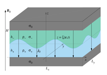
Figure 1: Sketch of the problem.

Consider a shallow rectangular cell of size $L_{x}\times L_{y}$ bounded horizontally by insulating sidewalls and vertically by two solid electrodes which are separated by a constant distance $H\ll L$, as shown in figure 1. The electrodes carry electric current of a constant density $\boldsymbol{j}_{0}=-j_{0}\boldsymbol{e}_{z}$ which passes through a layer of liquid metal (aluminium) of constant depth $\bar{h}_{+}$ and density $\rho_{+}$ superposed by a layer of electrolyte of depth $\bar{h}_{-}=H-\bar{h}_{+}$ and density $\rho_{-}<\rho_{+}$. The electrical conductivity of the liquid metal $\sigma_{+}$ is supposed to be much higher than that of the electrodes $\sigma_{0}$ which, in turn, is much higher than that of the electrolyte: $\sigma_{-}\ll\sigma_{0}\ll\sigma_{+}.$ This approximation, which is used already by Sneyd & Wang (1994), is applicable to aluminium reduction cells because $\sigma_{-}/\sigma_{0}\sim\sigma_{0}/\sigma_{+}\sim 10^{-2}$ (Gerbeau et al., 2006; Molokov et al., 2011).

The two-layer system is subject to a downward gravity force with the free fall acceleration $g$ and external magnetic field $\boldsymbol{B}_{0}=B_{0}\boldsymbol{e}_{z}$ which is assumed to be vertical and uniform. Horizontal components of the magnetic field, which are known to have a stabilizing effect as long as they are predominantly generated by the current passing through the system (Sneyd, 1985; Herreman et al., 2019), are as usual assumed to be negligible for the metal pad instability. This is because the effect of the horizontal magnetic field being determined by its horizontal gradient (Sneyd, 1985) is $\sim H/L=\varepsilon\ll 1$ relative to that of the vertical magnetic field which is determined by the magnitude of this field (Sneyd & Wang, 1994). The system admits a stably stratified quiescent equilibrium state with the layers separated by a plane horizontal interface. There is no electromagnetic force in this base state because the electric current is perfectly aligned with the magnetic field.

Note that a magnetostatic equilibrium in this system is in general possible if the magnetic field is vertically invariant. This, in turn, means that the vertical magnetic field, which is supposed to be generated by external currents, has to be also horizontally invariant (Sneyd & Wang, 1994). This is not the case in the model introduced by Urata et al. (1976) and also adopted by Bojarevics & Romerio (1994) who consider a horizontally inhomogeneous vertical component of the magnetic field but still assume a static base state.

Despite the highly idealised nature, this simple model captures the salient features of the Sele instability mechanism which is commonly believed to be relevant to aluminium reduction cells as well as to large-scale liquid metal batteries. For a comprehensive discussion of the relevance of the Sele instability mechanism (as well as a more more detailed analysis of the assumptions underlying this model), we refer the reader to Gerbeau et al. (2006, Sec. 6.1.4.3) who note the following: ‘Indeed, the model behind the Sele mechanism has been successfully used to improve the stability of some industrial cells (see [236]). In addition, the Sele mechanism has been confirmed by complete 3-D magnetohydrodynamic (MHD) simulations (see [99, 101, 179] and Section 6.3.3).’

Let us now consider a perturbed interface with the height $z=\zeta(\boldsymbol{x},t)$ which equals the depth of the bottom layer, $h_{+}(\boldsymbol{x},t)=\zeta(\boldsymbol{x},t)$, while the depth of the top layer is $h_{-}=H-h_{+}$. Following the shallow-water (long-wave) approximation, we assume that the perturbation has a characteristic longitudinal length scale $L\gg H$. Then the mass conservation implies that the vertical velocity $w$ is of relatively small magnitude $\sim H/L=\varepsilon\ll 1$. Respectively, the associated fluid flow is predominantly horizontal with the velocity $\boldsymbol{u}=u\boldsymbol{e}_{x}+v\boldsymbol{e}_{y}$. Such a flow has a negligible effect on the vertical pressure distribution which is thus purely hydrostatic:

$$p_{\pm}(\boldsymbol{x},z,t)=\mathit{\Pi}(\boldsymbol{x},t)+\rho_{\pm}g(\zeta-z),$$ (1)

where $\mathit{\Pi}(\boldsymbol{x},t)=\left.p_{\pm}(\boldsymbol{x},z,t)\right|_{z=\zeta}$ is the pressure distribution along the interface and $\boldsymbol{x}$ is the position vector in the $(x,y)$ plane. Substituting this pressure distribution into the horizontal fluid flow equation, we obtain

$$\rho(\partial_{t}\boldsymbol{u}+\boldsymbol{u}\cdot\boldsymbol{\nabla}\boldsymbol{u})=-\boldsymbol{\nabla}(\mathit{\Pi}+\rho g\zeta)+\boldsymbol{j}\times\boldsymbol{B},$$ (2)

where $\boldsymbol{j}$ is the current density and the $\pm$ indices are omitted for the sake of brevity.

The associated perturbation of the electric current density in each layer is governed by Ohm’s law for a moving medium

$$\boldsymbol{j}=\sigma(\boldsymbol{E}+\boldsymbol{u}\times\boldsymbol{B}),$$ (3)

where $\boldsymbol{E}$ is the perturbation of the electric field in the laboratory frame of reference. The oscillation period of interfacial waves, $\tau_{0}\sim L/c$, where $c$ is the wave speed (24), is assumed to be much longer than the characteristic magnetic diffusion time $\tau_{m}\sim\mu_{0}\sigma H^{2},$ where $\mu_{0}=4\pi\times 10^{-7}\,\mathrm{H/m}$ is the vacuum permeability. This is the case in aluminium reduction cells because $\tau_{m}/\tau_{0}\sim\mu_{0}\sigma cH^{2}/L\sim\varepsilon\mathit{Rm}\ll 1,$ where not only $\varepsilon=H/L$ but also the magnetic Reynolds number $\mathit{Rm=\mu_{0}\sigma cH}$ is usually small. It means that the induction effect due to the temporal variation of the magnetic field perturbation is negligible. Hence, the Faraday law of induction reduces to $\boldsymbol{\nabla}\times\boldsymbol{E}=0$, which corresponds to the so-called quasi-stationary or inductionless approximation commonly used in the liquid-metal MHD (Roberts, 1967). Then we have $\boldsymbol{E}=-\boldsymbol{\nabla}\varphi$, where $\varphi$ is the electric potential.

In addition, the perturbation of the electric field induced by the flow across the magnetic field, $\boldsymbol{u}\times\boldsymbol{B}$, is assumed to negligible relative to the horizontal electric field perturbation caused by the interface deformation. Using the charge conservation $\boldsymbol{\nabla}\cdot\boldsymbol{j}=0$, the latter can be estimated as $\sim j_{0}L/(\sigma H),$ whereas for the former we have $\sim B_{0}c,$ which thus leads to $HB_{0}c\sigma/(Lj_{0})\ll 1.$ For $B_{0}\sim\mu_{0}j_{0}L,$ this reduces to $\mathit{Rm}\ll 1,$ which, as noted above, is typically the case, and confirms the applicability of the aforementioned inductionless approximation. Note that in this approximation, also the magnetic field induced by the fluid flow is negligible relative to the external magnetic field. On the other hand, the perturbation of the vertical magnetic field component produced by the interface deformation with amplitude $\sim H$ can be evaluated as $\sim B_{0}H/L.$ Thus, we have $\boldsymbol{B}=B_{0}\boldsymbol{e}_{z}+O(\varepsilon,\mathit{Rm}).$

2.2 Reduction of the electric potential equation

Taking into account the above estimates, Ohm’s law (3) reduces to $\boldsymbol{j}=-\sigma\boldsymbol{\nabla}\varphi$ and, thus, the charge conservation $\boldsymbol{\nabla}\cdot\boldsymbol{j}=0$ results in

$$\boldsymbol{\nabla}^{2}\varphi=0,$$ (4)

which governs the electric potential in both layers. At the interface $z=\zeta(\boldsymbol{x},t)$, we have the continuity of both the potential and the normal component of electric current:

$$[\varphi]=[j_{n}]=0,$$ (5)

where $[f]$ stands for a jump of $f$ across the interface. The top electrode (anode) is assumed to be perfectly conducting relative to the electrolyte, which means that the interface between both is effectively equipotential. Since the electric potential is defined up an additive constant, we can set

$$\left.\varphi_{-}\right|_{z=H}=0.$$ (6)

As the electrical conductivity of the bottom electrode (cathode) is much lower than that of aluminium, the former may be regarded as effectively insulating with respect to internal current perturbations in the two-layer system. It means that the current density at the cathode is fixed

$$\left.\sigma_{+}\partial_{z}\varphi_{+}\right|_{z=0}=j_{0}.$$ (7)

Since $H/L=\varepsilon\ll 1$ the potential distribution in the aluminium layer can be approximated by the power series expansion in $z$ (Bojarevics & Romerio, 1994):

$$\varphi_{+}(\boldsymbol{r})=\phi_{+}^{(0)}(\boldsymbol{x})+z\phi_{+}^{(1)}(\boldsymbol{x})+\frac{z^{2}}{2}\phi_{+}^{(2)}(\boldsymbol{x})+O(\varepsilon^{3}),$$ (8)

where $\boldsymbol{x}=\boldsymbol{r}-z\boldsymbol{e}_{z}=x\boldsymbol{e}_{x}+y\boldsymbol{e}_{y}$ and $\phi_{+}^{(k)}(\boldsymbol{x})\equiv\left.\partial_{z}^{k}\varphi_{+}\right|_{z=0}$. Firstly, requiring (8) to satisfy (7) and (4), we find

$$\phi_{+}^{(1)} = j_{0}/\sigma_{+},$$ (9)

$$\phi_{+}^{(2)} = -\boldsymbol{\nabla}^{2}\phi_{+}^{(0)}+O(\varepsilon).$$ (10)

Secondly, using the interface normal

$$\boldsymbol{n}=\frac{\boldsymbol{e}_{z}-\boldsymbol{\nabla}h_{+}}{|\boldsymbol{e}_{z}-\boldsymbol{\nabla}h_{+}|}=\boldsymbol{e}_{z}-\boldsymbol{\nabla}h_{+}+\boldsymbol{e}_{z}O(\varepsilon^{2}),$$ (11)

the normal current at the interface can be expressed as

$$\left.j_{n}\right|_{z=h_{+}}=-\sigma_{+}\left.\partial_{n}\varphi_{+}\right|_{z=h_{+}}\approx-\sigma_{+}(\phi_{+}^{(1)}+h_{+}\phi_{+}^{(2)}-\boldsymbol{\nabla}h_{+}\cdot\boldsymbol{\nabla}\phi_{+}^{(0)})+O(\varepsilon^{2}).$$ (12)

Finally, substituting (9) and (10) into (12), after a few rearrangements, we obtain

$$\sigma_{+}\boldsymbol{\nabla}\cdot(h_{+}\boldsymbol{\nabla}\phi_{+}^{(0)})=j_{0}+\left.j_{n}\right|_{z=h_{+}}+O(\varepsilon^{2}),$$ (13)

which is a reduced two-dimensional potential equation for the aluminium layer.

In order to determine the normal current $\left.j_{n}\right|_{z=h_{+}}$ on the RHS of (13), we need to consider the potential distribution in the electrolyte layer, which can be sought as in the aluminium layer:

$$\varphi_{-}(\boldsymbol{r})=\phi_{-}^{(0)}(\boldsymbol{x})+(z-H)\phi_{-}^{(1)}(\boldsymbol{x})+\frac{1}{2}(z-H)^{2}\phi_{-}^{(2)}(\boldsymbol{x})+O(\varepsilon^{3}),$$ (14)

where $\phi_{-}^{(k)}(\boldsymbol{x})\equiv\left.\partial_{z}^{k}\varphi_{-}\right|_{z=H}$. Then applying (6) and (4), we find

$$\phi_{-}^{(0)}=\phi_{-}^{(2)}=0.$$ (15)

Similar to the top electrode, the aluminium layer is a much better conductor than the electrolyte layer. It means that the aluminium is effectively equipotential with respect to the electrolyte:

$$\left.\varphi_{-}\right|_{z=h_{+}}=(h_{+}-H)\phi_{-}^{(1)}(\boldsymbol{x})+O(\varepsilon^{3})=\varphi_{0},$$

where $\varphi_{0}$ is an unknown constant potential of the aluminium layer. As a result, we have

$$j_{z}=-\sigma_{-}\left.\partial_{z}\varphi_{-}\right|_{z=H}=\sigma_{-}\varphi_{0}/h_{-}+O(\varepsilon^{2}),$$

where $h_{-}=H-h_{+}$ is the depth of the electrolyte layer, and thus

$$\left.j_{n}\right|_{z=h_{+}}=j_{z}/n_{z}=j_{z}+O(\varepsilon^{2})=\sigma_{-}\varphi_{0}/h_{-}+O(\varepsilon^{2}).$$ (16)

Finally, substituting (16) into (13), we obtain

$$\sigma_{+}\boldsymbol{\nabla}\cdot(h_{+}\boldsymbol{\nabla}\phi_{+}^{(0)})=j_{0}+\sigma_{-}\varphi_{0}h_{-}^{-1},$$ (17)

which is accurate up to $O(\varepsilon^{2})$.

The unknown potential of the aluminium layer $\varphi_{0}$ is determined by the solvability condition of (17) which is required by the Neumann boundary condition at the insulating sidewalls where we have

$$\left.\partial_{n}\varphi_{+}\right|_{\Gamma}=\left.\partial_{n}\phi_{+}^{(0)}\right|_{\Gamma}+O(\varepsilon^{2})=0.$$ (18)

Integrating (17) over the horizontal cross-section area $S$ and using this boundary condition, we obtain

$$\int_{S}(j_{0}+\sigma_{-}\varphi_{0}h_{-}^{-1})\thinspace\mathrm{d}^{2}\boldsymbol{x}=0,$$

which is the solvability condition of (17). This condition, which requires the constancy of the total current $j_{0}S=I_{0}$, defines the potential of the aluminium layer

$$\varphi_{0}=-\sigma_{-}^{-1}I_{0}/\int_{S}h_{-}^{-1}\mathrm{d}^{2}\boldsymbol{x}.$$

Substituting this into (17), we obtain

$$\sigma_{+}\boldsymbol{\nabla}\cdot(h_{+}\boldsymbol{\nabla}\phi_{+}^{(0)})=j_{0}\left(1-Sh_{-}^{-1}/\int_{S}h_{-}^{-1}\mathrm{d}^{2}\boldsymbol{x}\right),$$ (19)

which is the final form of the reduced electric potential equation for the aluminium layer with the boundary condition (18).

Note that (19) is fully non-linear and, thus, applicable not only to small but also to large amplitude waves. Since the present linear stability analysis is concerned with the former, only the linearised version of (19) will be required in the following. Although the linear form of the potential equation has been derived and used in many previous studies, the full non-linear equation (19) is new to the best of our knowledge. For example, Bojarevics (1998) considers non-linear waves in aluminium electrolysis cells but uses linear potential equation (17) derived earlier by Bojarevics & Romerio (1994). Equation (19) differs also from analogous equation (11) of Zikanov et al. (2000). Instead of expanding the potential in powers of $z$, which is essential in this case (Bojarevics & Romerio, 1994), they integrate a three-dimensional potential equation over the depth of the aluminium layer. As this operation cannot consistently be carried through, Zikanov et al. (2000) effectively postulate that the integral of the horizontal current over the depth of the aluminium layer can be written as $\boldsymbol{J}=-\sigma_{+}\boldsymbol{\nabla}\Psi,$ whereas we have $\boldsymbol{J}=-\sigma_{+}h_{+}\boldsymbol{\nabla}\phi_{+}^{(0)},$ which follows from Ohm’s law and the $z$-invariance of $\phi_{+}^{(0)}.$ Both expressions are equivalent only for small-amplitude waves when $h_{+}\approx\bar{h}_{+}=\text{const}$ and, thus, $\Psi=\bar{h}_{+}\phi_{+}^{(0)}.$ Consequently, equation (11) of Zikanov et al. (2000) is limited to small-amplitude waves.

2.3 Linearised shallow-water model

The distribution of the electric potential in the aluminium layer (8) indicates that the respective electromagnetic force

$$\boldsymbol{j_{+}}\times\boldsymbol{B_{0}}=\sigma_{+}\boldsymbol{B_{0}}\times\boldsymbol{\nabla}\phi_{+}^{(0)}(\boldsymbol{x})+O(\varepsilon^{2})$$

is depth invariant up to $O(\varepsilon^{2})$. Since the curl of this force has zero horizontal components, it preserves zero horizontal vorticity of the flow. In the hydrostatic shallow-water approximation, when the vertical velocity component is negligible, this is equivalent to the depth invariance of the horizontal velocity: $\partial_{z}\boldsymbol{u}\equiv 0$. Consequently, this electromagnetic force is compatible with the conservation of the depth invariance which is a generic property of the two-layer shallow-water system (Priede, 2020). In the electrolyte layer, according to (14) and (15), the horizontal component of the current perturbation and, thus, also the associated electromagnetic force is $O(\varepsilon)$, i.e. negligible in the hydrostatic shallow-water approximation. Therefore, the conservation of the depth invariance holds also in the electrolyte layer.

The system of shallow-water equations is closed by adding the conservation of mass in each layer:

$$\partial_{t}h+\boldsymbol{\nabla}\cdot(h\boldsymbol{u})=0,$$ (20)

which is obtained by integrating the incompressibility constraint $\boldsymbol{\nabla}\cdot\boldsymbol{u}=0$ over the depth of the respective layer and using the kinematic constraint at the interface $z=\zeta(\boldsymbol{x},t):$

$$\frac{d\zeta}{dt}=\partial_{t}\zeta+\boldsymbol{u}\cdot\boldsymbol{\nabla}\zeta=w.$$

In the following, we focus on the interfacial waves of small amplitude:

$$\eta(\boldsymbol{x},t)=\zeta(\boldsymbol{x},t)-\bar{h}_{+}\ll H.$$

It means that the nonlinear terms in the governing equations are higher-order small and, thus, negligible relative to the linear terms. After linearisation, (2) and (20) take the form

$$\rho_{\pm}\partial_{t}\boldsymbol{u}_{\pm} = -\boldsymbol{\nabla}(\mathit{\Pi}+\rho_{\pm}g\eta)+\sigma_{\pm}\boldsymbol{B}_{0}\times\boldsymbol{\nabla}\phi_{\pm}^{(0)},$$ (21)

$$\partial_{t}\eta = \mp\bar{h}_{\pm}\boldsymbol{\nabla}\cdot\boldsymbol{u}_{\pm}.$$ (22)

Taking the divergence of the difference of equations (21) for the top and bottom layers, which correspond to the plus and minus indices, and using (22), we obtain the classical wave equation

$$\partial_{t}^{2}\eta=c^{2}\boldsymbol{\nabla}^{2}\eta,$$ (23)

for interfacial gravity waves propagating with the speed

$$c=\left(\frac{g(\rho_{+}-\rho_{-})}{\rho_{+}/\bar{h}_{+}+\rho_{-}/\bar{h}_{-}}\right)^{1/2}.$$ (24)

Note that since the electromagnetic force is entirely solenoidal, i.e. $\boldsymbol{B}_{0}\times\boldsymbol{\nabla}\phi_{\pm}^{(0)}=-\boldsymbol{\nabla}\times\phi_{\pm}^{(0)}\boldsymbol{B}_{0}$, it can drive a flow without disturbing pressure as long as the flow is not obstructed by the sidewalls. It implies that the electromagnetic force can affect interfacial waves only at the sidewalls. The boundary condition for (23) follows from $\left.u_{n}\right|_{\mathit{\Gamma}}=0$ which holds at the impermeable sidewall $\mathit{\Gamma}$. Taking again the difference of equations (21) for the top and bottom layers to eliminate the pressure and then applying the impermeability condition, we obtain

$$\left.g[\rho]\partial_{n}\eta\right|_{\mathit{\Gamma}}=\left.B_{0}\partial_{\tau}[\sigma\phi^{(0)}]\right|_{\mathit{\Gamma}},$$ (25)

where $\partial_{n}\equiv\boldsymbol{n}\cdot\boldsymbol{\nabla}$ and $\partial_{\tau}\equiv\boldsymbol{\tau}\cdot\boldsymbol{\nabla}$ with $\boldsymbol{n}$ and $\boldsymbol{\tau}=\boldsymbol{n}\times\boldsymbol{e}_{z}$ standing for the outward normal and tangent vectors to the lateral cell boundary $\mathit{\Gamma};$ the square brackets denote the difference of the enclosed quantity between the top and bottom layers.

After linearisation, that is, applying

$$h_{+} = \bar{h}_{+}+\eta\approx\bar{h}_{+},$$

$$h_{-}^{-1} = (\bar{h}-\eta)^{-1}\approx\bar{h}_{-}^{-1}+\eta\bar{h}_{-}^{-2},$$

and taking into account that $\int_{s}\eta\thinspace\mathrm{d}^{2}\boldsymbol{x}=0$ due to the mass conservation, the potential equation (19) reduces to

$$\boldsymbol{\nabla}^{2}\phi_{+}^{(0)}=-\frac{j_{0}\eta}{\sigma_{+}\bar{h}_{+}\bar{h}_{-}},$$ (26)

which satisfies the solvability condition automatically owing to the mass conservation. This equation originally formulated by Urata et al. 1976 differs from the analogous equation derived later by Bojarevics & Romerio (1994) by the absence of terms containing the ratio of electric conductivities of electrolyte and aluminium, $\sim\sigma_{-}/\sigma_{+}\sim 10^{-4},$ which is $\sim(H/L)^{2},$ i.e. comparable to the higher-order-small terms usually neglected in the hydrostatic shallow-water approximation (Lukyanov et al., 2001).

Henceforth, we change to dimensionless variables by using $L=\sqrt{L_{x}L_{y}}=S^{1/2}$, $\tau_{0}=L/c$ and $\phi_{0}=I_{0}/(\sigma_{+}\bar{h}_{+})$ as the length, time and electric potential scales, respectively. The dimensionless governing equations (23) and (26) read as

$$\partial_{t}^{2}\eta+\gamma\partial_{t}\eta = \boldsymbol{\nabla}^{2}\eta,$$ (27)

$$-\eta = \boldsymbol{\nabla}^{2}\phi,$$ (28)

where $\phi$ is the dimensionless counterpart of $\phi_{+}^{(0)}$. Note that following Lukyanov et al. (2001), we have added a linear damping (viscous friction) term to (27) defined by a phenomenological friction parameter $\gamma$. The latter is subsequently assumed to be small and, thus, ignored, unless stated otherwise. The dimensionless boundary conditions corresponding to (18) and (25) are

$$\left.\partial_{n}\eta\right|_{\mathit{\Gamma}} = \beta\left.\partial_{\tau}\phi\right|_{\mathit{\Gamma}},$$ (29)

$$\left.\partial_{n}\phi\right|_{\mathit{\Gamma}} = 0,$$ (30)

where

$$\beta=\frac{I_{0}B_{0}}{g(\rho_{+}-\rho_{-})\bar{h}_{+}\bar{h}_{-}}$$ (31)

is the key dimensionless parameter for this problem, referred to by Gerbeau et al. (2006) as the Sele number (Sele, 1977), which defines the strength of electromagnetic force relative to that of gravity.

3 Linear stability analysis

3.1 Eigenvalue perturbation solution for $\beta\ll 1$

Let us now turn to the linear stability problem posed by (27) and (28) for a rectangular cell of aspect ratio $\alpha=L_{x}/L_{y}$ which is bounded laterally by four sidewalls. Although the problem does not admit an exact analytical solution as for the semi-infinite and channel geometries (see appendix A), it can still be solved approximately for sufficiently small $\beta$ using the classical eigenvalue perturbation method (Hinch, 1991, Sec. 1.6). To this end, the eigenmode

$$\{\eta,\phi\}(\boldsymbol{x},t)=\{\hat{\eta},\hat{\phi}\}(\boldsymbol{x})e^{-i\omega t}+\text{c.c.},$$ (32)

where c.c. stands for the complex conjugate, is sought by expanding the eigenvalue $\omega^{2}$ and the respective amplitude distribution in the power series of $\beta:$

$$\omega^{2} = \lambda^{(0)}+\beta\lambda^{(1)}+\ldots,$$ (33)

$$\{\hat{\eta},\hat{\phi}\}(\boldsymbol{x}) = \{\hat{\eta},\hat{\phi}\}^{(0)}(\boldsymbol{x})+\beta\{\hat{\eta},\hat{\phi}\}^{(1)}(\boldsymbol{x})+\ldots.$$ (34)

At the leading order, which corresponds to $\beta=0$, (27)–(30) reduce to

$$\lambda^{(0)}\hat{\eta}^{(0)}+\boldsymbol{\nabla}^{2}\hat{\eta}^{(0)}=0, \left.\partial_{n}\hat{\eta}^{(0)}\right|_{\mathit{\Gamma}}=0,$$ (35)

$$\hat{\eta}^{(0)}+\boldsymbol{\nabla}^{2}\hat{\phi}^{(0)}=0, \left.\partial_{n}\hat{\phi}^{(0)}\right|_{\mathit{\Gamma}}=0.$$ (36)

The respective leading-order solution is

$$\lambda_{\boldsymbol{k}}^{(0)} = \boldsymbol{k}^{2},$$ (37)

$$\{\hat{\eta},\hat{\phi}\}^{(0)}(\boldsymbol{x}) = \{\boldsymbol{k}^{2},1\}\hat{\phi}{}_{\boldsymbol{k}}^{(0)}\Psi_{\boldsymbol{k}}(\boldsymbol{x}),$$ (38)

where

$$\Psi_{\boldsymbol{k}}(\boldsymbol{x})=\cos(xk_{x})\cos(yk_{y})$$ (39)

is the gravity wave mode with the wave vector

$$\boldsymbol{k}=(k_{x},k_{y})=\pi(m/\sqrt{\alpha},n\sqrt{\alpha}),\,\,m,n=0,1,2,\ldots$$ (40)

It is important to note that some leading-order eigenmodes (38) may be degenerate, namely, to have the same eigenfrequency (37) for different wave vectors. In this case, the leading-order solution can be a superposition of the eigenmodes (38) with the same magnitude of the wave vector $\boldsymbol{k}^{\prime 2}=\boldsymbol{k}^{2}:$

$$\{\hat{\eta},\hat{\phi}\}^{(0)}(\boldsymbol{x})={\displaystyle\sum_{\boldsymbol{\boldsymbol{k}^{\prime 2}=\boldsymbol{k}^{2}}}\{\hat{\eta},\hat{\phi}\}_{\boldsymbol{k^{\prime}}}^{(0)}\Psi_{\boldsymbol{k^{\prime}}}(\boldsymbol{x}).}$$ (41)

Following the standard approach, the first-order correction $\{\hat{\eta},\hat{\phi}\}^{(1)}$ to (41) is sought as an expansion in the leading-order eigenmodes

$$\{\hat{\eta},\hat{\phi}\}^{(1)}(\boldsymbol{x})={\displaystyle\sum_{\boldsymbol{k}}\{\hat{\eta},\hat{\phi}\}_{\boldsymbol{k}}^{(1)}\Psi_{\boldsymbol{k}}(\boldsymbol{x}),}$$

where the summation is over all wave vectors. Substituting this expansion into the first-order problem

$$\lambda^{(0)}\hat{\eta}^{(1)}+\boldsymbol{\nabla}^{2}\hat{\eta}^{(1)}=-\lambda^{(1)}\hat{\eta}^{(0)}, \left.\partial_{n}\hat{\eta}^{(1)}\right|_{\mathit{\Gamma}}=\left.\partial_{\tau}\hat{\phi}^{(0)}\right|_{\mathit{\Gamma}},$$ (42)

$$\hat{\eta}^{(1)}+\boldsymbol{\nabla}^{2}\hat{\phi}^{(1)}=0, \left.\partial_{n}\hat{\phi}^{(1)}\right|_{\mathit{\Gamma}}=0.$$ (43)

and using the orthogonality of leading-order eigenmodes by projecting the result onto $\Psi_{\boldsymbol{k}}$, after a few rearrangements, we obtain the solvability condition of the first-order problem

$${\displaystyle\lambda_{\boldsymbol{k}}^{(1)}\boldsymbol{k}^{2}\left\langle\Psi_{\boldsymbol{k}}^{2}\right\rangle\hat{\phi}_{\boldsymbol{k}}^{(0)}-\sum_{\boldsymbol{k}^{\prime 2}=\boldsymbol{k}^{2}}}F_{\boldsymbol{k},\boldsymbol{k}^{\prime}}\hat{\phi}_{\boldsymbol{k}^{\prime}}^{(0)}=(\boldsymbol{k}^{2}-\lambda_{\boldsymbol{k}}^{(0)})\boldsymbol{k}^{2}\left\langle\Psi_{\boldsymbol{k}}^{2}\right\rangle\hat{\phi}_{\boldsymbol{k}}^{(1)}=0,$$ (44)

where the right-hand side is zero owing to the leading-order solution (37) and, thus, the left-hand side defines the eigenvalue perturbation $\lambda_{\boldsymbol{k}}^{(1)}.$ The summation on the left-hand side is over the degenerate modes as in (41); for non-degenerate modes, it reduces to a single term with $\boldsymbol{k}^{\prime}=\boldsymbol{k}$. The angle brackets denote integral over $S=L_{x}\times L_{y}:$

$$\left\langle\Psi_{\boldsymbol{k}}^{2}\right\rangle={\displaystyle\int_{S}\Psi_{\boldsymbol{k}}^{2}\thinspace\mathrm{d}^{2}\boldsymbol{x}}=c_{k_{x}}^{-1}c_{k_{y}}^{-1},$$

where $c_{0}=1$ and $c_{k}=2$ for $k\not=0$. The second left-hand side term of (44) is due to Green’s first identity

$$\left\langle\Psi_{\boldsymbol{k}}\boldsymbol{\nabla}^{2}\hat{\eta}^{(1)}+\boldsymbol{\nabla}\Psi_{\boldsymbol{k}}\cdot\boldsymbol{\nabla}\hat{\eta}^{(1)}\right\rangle=\ointop_{\mathit{\Gamma}}\Psi_{\boldsymbol{k}}\partial_{n}\hat{\eta}^{(1)}\mathrm{d}\mathit{\Gamma},$$

where the boundary integral can be transformed using the boundary condition (42) and Green’s theorem as follows:

$$\ointop_{\mathit{\Gamma}}\Psi_{\boldsymbol{k}}\partial_{\tau}\hat{\phi}^{(0)}\mathrm{d}\mathit{\Gamma}=-\left\langle\boldsymbol{e}_{z}\cdot\boldsymbol{\nabla}\Psi_{\boldsymbol{k}}\times\boldsymbol{\nabla}\hat{\phi}^{(0)}\right\rangle.$$

This results in the electromagnetic interaction matrix

$$F_{\boldsymbol{k},\boldsymbol{k}^{\prime}}=\left\langle\boldsymbol{e}_{z}\cdot\boldsymbol{\nabla}\Psi_{\boldsymbol{k}}\times\boldsymbol{\nabla}\Psi_{\boldsymbol{k}^{\prime}}\right\rangle=G_{\boldsymbol{k},\boldsymbol{k}^{\prime}}-G_{\boldsymbol{k}^{\prime},\boldsymbol{k}},$$ (45)

where $G_{\boldsymbol{k},\boldsymbol{k}^{\prime}}=H_{k_{x},k_{x}^{\prime}}H_{k_{y}^{\prime},k_{y}}$ and

$$H_{k_{m},k_{n}}=k_{m}\left\langle\sin(xk_{m})\cos(xk_{n})\right\rangle=\frac{2m^{2}}{m^{2}-n^{2}}\text{mod}(m+n,2),$$ (46)

Expressions (45) and (46) differ form of those used by Sneyd & Wang (1994) only by a more compact form.

Since the electromagnetic interaction matrix (45) is anti-symmetric, as it is well known, there is no electromagnetic back-reaction on separate gravity wave modes, i.e. $F_{\boldsymbol{k},\boldsymbol{k}}=0$. Thus, for a non-degenerate (single) mode, we have

$$\lambda_{\boldsymbol{k}}^{(1)}\left\langle\Psi_{\boldsymbol{k}}^{2}\right\rangle k^{2}\hat{\phi}_{\boldsymbol{k}}=F_{\boldsymbol{k},\boldsymbol{k}}\hat{\phi}_{\boldsymbol{k}}=0,$$

which means no electromagnetic effect at the first order in $\beta$. For a degenerate mode consisting of a superposition of two eigenmodes with the same frequency

$$\lambda_{\boldsymbol{k}}^{(0)}=\boldsymbol{k}_{1}^{2}=\boldsymbol{k}_{2}^{2},$$ (47)

equation (44) can be written in the matrix form as

$$\lambda_{\boldsymbol{k}}^{(1)}k^{2}\left(\begin{array}[]{c}\left\langle\Psi_{\boldsymbol{k}_{1}}^{2}\right\rangle\hat{\phi}_{\boldsymbol{k_{1}}}\\ \left\langle\Psi_{\boldsymbol{k}_{2}}^{2}\right\rangle\hat{\phi}_{\boldsymbol{k}_{2}}\end{array}\right)=\left(\begin{array}[]{cc}0&F_{\boldsymbol{k}_{1},\boldsymbol{k}_{2}}\\ -F_{\boldsymbol{k}_{1},\boldsymbol{k}_{2}}&0\end{array}\right)\left(\begin{array}[]{c}\hat{\phi}_{\boldsymbol{k}_{1}}\\ \hat{\phi}_{\boldsymbol{k}_{2}}\end{array}\right).$$ (48)

The solution of this second-order matrix eigenvalue problem yields

$$\lambda_{\boldsymbol{k}}^{(1)}k^{2}\sqrt{\left\langle\Psi_{\boldsymbol{k}_{1}}^{2}\right\rangle\left\langle\Psi_{\boldsymbol{k}_{2}}^{2}\right\rangle}=\pm iF_{\boldsymbol{k}_{1},\boldsymbol{k}_{2}},$$ (49)

which indicates that $\lambda_{\boldsymbol{k}}^{(1)}$ is imaginary and, thus, the system is unstable provided that $F_{\boldsymbol{k_{1}},\boldsymbol{k}_{2}}\not=0$. According to (46), this is the case only if both components of the two wave vectors $\boldsymbol{k}_{1`}=\pi(m_{1}/\sqrt{\alpha},n_{1}\sqrt{\alpha})$ and $\boldsymbol{k}_{2}=\pi(m_{2}/\sqrt{\alpha},n_{2}\sqrt{\alpha})$ have opposite parities; namely, $m_{1}\pm m_{2}$ and $n_{1}\pm n_{2}$ are odd numbers. Then the degeneracy condition (47) yields

$$\alpha_{c}^{2}=-\frac{(m_{1}+m_{2})(m_{1}-m_{2})}{(n_{1}+n_{2})(n_{1}-n_{2})}=\frac{m}{n},$$

where $m$ and $n$ can be any odd numbers. Consequently, all cells with aspect ratios squared equal to the ratio of two odd numbers are inherently unstable, i.e. they become unstable at infinitesimal $\beta>\beta_{c}=0$.

For $\alpha^{2}=1$, which corresponds to a square cell, the unstable wavenumbers are $m_{1}=l,\,n_{1}=0$ and $m_{2}=0,\,n_{2}=l$, where $l=1,3,5,\ldots$. In this case, (49) yields $\lambda_{l}^{(1)}=\pm i8/(l\pi)^{2}$ and hence the instability growth rate resulting from (33) is

$$\Im[\omega_{l}^{(1)}]=\pm\frac{4}{(l\pi)^{3}},$$ (50)

which means that the most unstable is the mode with $l=1$. For a general $\alpha^{2}=m/n$ defined by arbitrary odd numbers $m$ and $n$, the lowest unstable wavenumbers can be written as

$$m_{(3\pm 1)/2} = (m\pm 1)/2,$$ (51)

$$n_{(3\pm 1)/2} = (n\mp 1)/2.$$ (52)

In this case, (49) yields $\lambda_{m,n}^{(1)}=\pm i8c_{m-1}^{1/2}c_{n-1}^{1/2}/(\pi^{2}\sqrt{mn})$ and, respectively, (33) results in

$$\Im[\omega_{m,n}^{(1)}]=\pm\frac{8}{\pi^{3}}\left(\frac{c_{m-1}c_{n-1}}{(m+n)(1+mn)\sqrt{mn}}\right)^{1/2},$$ (53)

which reduces to (50) with $l=1$ when $m=n=1$. It is important to note that the growth rate (53) drops off with the increase of $m$ and $n$ as $\sim(m+n)^{-1/2}(mn)^{-3/4}.$

For an aspect ratio $\alpha$ sufficiently close to the critical value $\alpha_{c}=\sqrt{m/n},$ the stability of system is expected to be determined by the interaction of two critical modes with the wavenumbers $($51,52) which correspond to the wavenumbers

$$\boldsymbol{k}_{(3\pm 1)/2}=\frac{\pi}{2}((m\pm 1)/\sqrt{\alpha},(n\mp 1)\sqrt{\alpha}).$$

Searching the amplitude distribution in (32) as

$$\{\hat{\eta},\hat{\phi}\}(\boldsymbol{x})=\{\hat{\eta},\hat{\phi}\}_{\boldsymbol{k}_{1}}\Psi_{\boldsymbol{k}_{1}}+\{\hat{\eta},\hat{\phi}\}_{\boldsymbol{k}_{2}}\Psi_{\boldsymbol{k}_{2}},$$

without assuming $\beta$ to be small, we obtain the following second-order matrix eigenvalue problem for $\omega^{2}:$

$$\left(\begin{array}[]{cc}(\omega^{2}-\boldsymbol{k}_{1}^{2})\boldsymbol{k}_{1}^{2}&\beta F_{\boldsymbol{k}_{1},\boldsymbol{k}_{2}}c_{n-1}\\ -\beta F_{\boldsymbol{k}_{1},\boldsymbol{k}_{2}}c_{m-1}&(\omega^{2}-\boldsymbol{k}_{2}^{2})\boldsymbol{k}_{2}^{2}\end{array}\right)\left(\begin{array}[]{c}\hat{\phi}_{\boldsymbol{k}_{1}}\\ \hat{\phi}_{\boldsymbol{k}_{2}}\end{array}\right)=\mathsf{\mathbf{0}},$$ (54)

where $F_{\boldsymbol{k}_{1},\boldsymbol{k}_{2}}=2(m+n)(mn+1)/(mn)$. As before, for the system to be stable, the eigenvalue $\omega^{2}$ has to be real. This is the case if $\beta\leq\beta_{m,n}(\alpha^{2})$, where

$$\beta_{m,n}(\alpha^{2})= \frac{\pi^{4}}{16}\frac{\left|\alpha_{c}^{2}/\alpha{}^{2}-1\right|mn^{2}}{(m+n)(mn+1)}$$

$$\times \left(\frac{(m^{2}-1)^{2}+\alpha^{4}(n^{2}-1)^{2}+2\alpha^{2}((m+n)^{2}+(mn+1)^{2})}{c_{m-1}c_{n-1}}\right)^{1/2}.$$ (55)

For aspect ratios with $\alpha^{2}=m$, where $m$ is an even number, using the two-mode approximation (55) for the preceding major critical point, i.e. $\alpha_{c}^{2}=m-1$, we have

$$\beta_{m-1,1}(m)=\frac{\pi^{4}}{16}\frac{(m-1)}{m^{2}}\sqrt{\frac{m^{2}+4}{c_{m-2}}}.$$

The lowest $\beta_{m-1,1}=\frac{3\pi^{4}}{128}\sqrt{\frac{5}{2}}\approx 3.61$ occurs at $m=4$, whereas the highest $\beta_{m-1,1}=\frac{\pi^{4}}{16\sqrt{2}}\approx 4.30$ at $m=2$, which is then approached asymptotically at large even $m$.

The intersection of instability thresholds associated with the first two major critical points, which is defined by $\beta_{1,1}(\alpha^{2})=\beta_{3,1}(\alpha^{2})$, yields $\alpha_{c}^{2}\approx 2.125$ and, thus, in the two-mode approximation, we have $\beta_{c}\approx 4.699$. As shown in the next section, this is the optimal aspect ratio and the corresponding highest stability threshold which can be achieved with a small viscous friction.

3.2 Numerical solution of the matrix eigenvalue problem

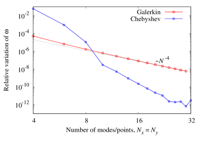
Figure 2: The relative variation of the complex frequency with the largest imaginary part ($\omega=3.14455+\mathrm{i}0.12889)$ versus the number of modes and nodes used in the Galerkin and Chebyshev approximations for $\alpha=\beta=1$.

For arbitrary $\beta$, (32) leads to

$$\lambda\hat{\eta}+\boldsymbol{\nabla}^{2}\hat{\eta}=0, \left.\partial_{n}\hat{\eta}\right|_{\mathit{\Gamma}}=\beta\left.\partial_{\tau}\hat{\phi}\right|_{\mathit{\Gamma}},$$ (56)

$$\hat{\eta}+\boldsymbol{\nabla}^{2}\hat{\phi}=0, \left.\partial_{n}\hat{\phi}\right|_{\mathit{\Gamma}}=0,$$ (57)

which is an eigenvalue problem for $\lambda=\omega^{2}+\mathrm{i}\gamma$, where $\gamma$ is a viscous friction coefficient. The problem can be discretised using the Galerkin method with the gravity wave modes (39) as basis functions. This leads to the generalisation of (44):

$$(\lambda-\boldsymbol{k}^{2})\boldsymbol{k}^{2}\left\langle\Psi_{\boldsymbol{k}}^{2}\right\rangle\hat{\phi}_{\boldsymbol{k}}=\beta{\displaystyle\sum_{\boldsymbol{k}^{\prime}}}F_{\boldsymbol{k},\boldsymbol{k}^{\prime}}\hat{\phi}_{\boldsymbol{k}^{\prime}},$$

with the electromagnetic interaction matrix on the right-hand side defined by (45). This is a matrix eigenvalue problem of size $(M+1)^{2}\times(N+1)^{2}$, where $M$ and $N$ are the cutoff limits of the $x$- and $y$-components of the wave vectors (40). This method with $M\times N=12$ modes was used by Sneyd & Wang (1994) to compute the stability threshold for a cell of length $7.7\,\mathrm{m}$ depending on the width which varied from $\approx 0.5\,\mathrm{m}$ to $8\,\mathrm{m}.$ Alternatively, (56,57) can be discretised using the Chebyshev collocation method (Boyd, 2013) (see appendix B). As seen in figure 2, the latter has a significantly faster convergence rate than $\sim N^{-4}$ achieved by the Galerkin approximation with $N$ modes in each direction. As the relative accuracy of the Chebyshev collocation approximation saturates at $\approx 10^{-11}\cdots 10^{-12}$ when $N\apprge 24$, in the following, we use $16\cdots 24$ collocation points in each direction.

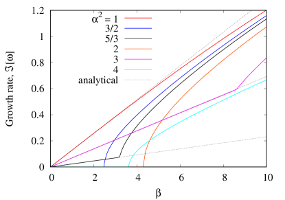
Figure 3: The highest growth rate $\Im[\omega]$ depending on the interaction parameter $\beta$ for various aspect ratios $\alpha$ computed by the Chebyshev collocation method with $N_{x}=N_{y}=16$. For $\alpha^{2}=m/n$, where $m$ and $n$ are odd numbers, numerical results are compared with the approximate analytical solution (53).

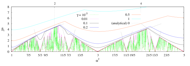
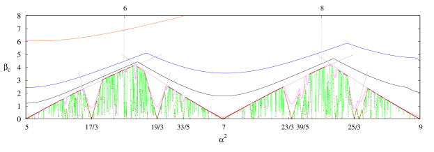
Figure 4: Instability threshold $\beta_{c}$ depending on the aspect ratio squared $(\alpha^{2})$ computed for various viscous friction coefficients $\gamma$ using Chebyshev collocation method with $N_{x}=N_{y}=16\cdots 24$ points. Analytical solution (55) is plotted for the dominant critical points $\alpha_{c}^{2}$ equal to odd numbers and their thirds.

The highest growth rate $\omega_{i}=\Im[\omega]$, which is computed using Chebyshev collocation method with $N_{x}=N_{y}=16$ points and plotted in figure 3 against the interaction parameter $\beta$ for various aspect ratios $\alpha$, confirms the eigenvalue perturbation solution obtained in the previous section. Namely, for $\alpha^{2}$ equal to the ratio of two odd numbers, the growth rate becomes positive at $\beta>\beta_{c}=0$ whereas for other aspect ratios this happens only at finite $\beta_{c}$. The dependence of the instability threshold $\beta_{c}$ on $\alpha^{2}$ is shown in figure 4 for various viscous friction coefficients $\gamma$. Note that the instability threshold cannot be computed for $\gamma=0$ because it becomes absolutely fractal in this limit. Due to the finite accuracy of numerical solution, the lowest friction coefficient for which the stability threshold can reliably be computed is around $\gamma=10^{-5}.$ For this value, the stability diagram is very rugged and exhibits both small- and large-scale patterns. The key feature are the dips in $\beta_{c}$ which can be seen to occur at $\alpha_{c}^{2}$ equal to the ratio of two odd numbers as predicted by the eigenvalue perturbation analysis in the previous section. The increase of the friction coefficient $\gamma$ gradually smooths out the dependence of $\beta_{c}$ on $\alpha$, especially at small scales and larger aspect ratios. However, the main feature of the stability diagram, which is the location of minima and maxima of $\beta_{c}$ in the vicinity of odd and even values of $\alpha^{2}$, respectively, persists up to relatively large friction coefficients $\gamma\sim 0.1$. It is remarkable that the approximate solution (55) for the major critical points closely reproduces the numerical results obtained with $N_{x}=N_{y}=24$ collocation points. According to the approximate solution obtained in the previous section, the first four maxima of $\beta_{c}\approx 4.70,4.11,4.19,4.23$ are located at $\alpha^{2}\approx 2.13,4.16,6.12,8.10$.

4 Summary and discussion

We have carried out a comprehensive linear stability analysis of interfacial waves in the idealised model of an aluminium reduction cell. The model consists of two stably stratified liquid layers carrying a vertical electric current in the presence of a uniform collinear external magnetic field. Using the long-wave approximation, we derived a fully nonlinear shallow-water model comprising a novel integro-differential equation for the electric potential. Our shallow-water model differs from that of Bojarevics (1998) by being fully nonlinear and, thus, applicable not only to small but also to large amplitude waves. It should also be noted that the electric potential equation we derived differs from that postulated by Zikanov et al. (2000). The nonlinear potential equation is just a side result which may be useful for numerical modelling of large amplitude shallow-water waves but it is not essential for the linear stability analysis of infinitesimal amplitude waves considered in the present study.

In this study, we showed that rectangular cells are inherently unstable if their aspect ratio squared equals the ratio of two odd numbers: $\alpha^{2}=m/n.$ In the inviscid limit, such cells can be destabilised by an infinitesimally weak electromagnetic interaction while cells with other aspect ratios have finite instability thresholds. The unstable aspect ratios form an absolutely discontinuous dense set of points which intersperse aspect ratios with finite stability thresholds. This inherent fractality of the instability threshold was revealed analytically using an eigenvalue perturbation method and confirmed by accurate numerical solution of the underlying linear stability problem.

Although the instability threshold is gradually smoothed out by viscous friction, its principal structure, which is dominated by major critical aspect ratios corresponding to moderate values of $m$ and $n$, is well preserved up to relatively large dimensionless linear damping coefficients $\gamma\sim 0.1$. For $\gamma\lesssim 1,$ cells with such aspect ratios have the lowest stability threshold with the critical electromagnetic parameter $\beta_{c}\sim\gamma,$ while the most stable are cells with $\alpha^{2}\approx 2.13$ which have $\beta_{c}\approx 4.7.$

For a reduction cell operated at a total electric current of $I_{0}\approx 300\,\mathrm{kA}$ with the electrolyte and aluminium layers of depth $\bar{h}_{-}\approx 5\,\mathrm{cm}$ and $\bar{h}_{+}\approx 25\,\mathrm{cm}$, respectively, and the density difference $\Delta\rho=\rho_{+}-\rho_{-}\approx 200\,\mathrm{kg/m^{3},}$ this $\beta_{c}$ corresponds to the critical magnetic field

$$B_{0}=\beta_{c}g\Delta\rho\bar{h}_{+}\bar{h}_{-}/I_{0}\approx 0.27\,\mathrm{mT}.$$

This field is an order of magnitude stronger than Earth’s magnetic field but still an order of magnitude weaker than the magnetic fields which can be generated by the electric current flowing in the reduction cell itself and in the adjacent cells. It should be noted that it is not the whole magnetic field but only its vertical component which is important for the metal pad instability.

It is also important to note that the above result is based on the assumption of a relatively small linear damping in the two-layer system, i.e. $\gamma\sim\tau_{0}/\tau_{\nu}\lesssim 0.1$, where $\tau_{0}$ and $\tau_{\nu}$ are the characteristic wave propagation and viscous damping times with the latter being the reciprocal of the linear friction coefficient. For a cell with $L_{x}L_{y}\approx 40\,\mathrm{m^{2}}$ and $c\approx 0.2\,\mathrm{m/s,}$ we have $\tau_{0}=L/c\sim 10\,\mathrm{s.}$ Viscous damping is expected to be dominated by the electrolyte layer, which is thinner and also more viscous than the aluminium layer. Using $\nu_{-}\sim 10^{-6}\,\mathrm{m^{2}/s}$ as a characteristic kinematic viscosity of cryolite (Hertzberg et al., 2013), we obtain $\tau_{\nu}\sim\bar{h}_{-}^{2}/\nu_{-}\sim 10^{3}\,\mathrm{s}$. On the other hand, assuming $B_{0}\sim 1\,\mathrm{mT,}$we obtain the same order-of-magnitude magnetic damping time in the aluminium layer: $\tau_{m}\sim\rho_{+}/\sigma_{+}B_{0}^{2}\sim 10^{3}\,\mathrm{s}$. Consequently, we have $\gamma\sim 10^{-2}$ for both the viscous and the magnetic damping. This, however, is at odds with the customary assumption that the viscous damping time in real reduction cells is $\tau_{\nu}\sim 10\,\mathrm{s}$ and, thus, $\gamma\sim 1$ (Moreau & Ziegler, 1988; Zikanov et al., 2000; Molokov et al., 2011).

Such a high damping may be due to turbulence which is likely to develop when the waves become sufficiently large. Damping can also be affected by the large-scale circulation which occurs in real cells due to the non-uniformity of electric current and magnetic field. The same non-uniformity can also affect the instability threshold directly by modifying the electromagnetic coupling strength of different gravity wave modes. These, however, are rather complex effects which are outside the scope of the basic Sele instability model. Nevertheless, this model is still relevant to the stability of real aluminium reduction cells as confirmed by complete 3-D MHD simulations (Gerbeau et al., 2006, Sec. 6.1.4.3 and references therein).

When the background circulation is negligible, which is usually assumed to be the case in this model, the waves can have a sufficiently small initial amplitude for the linear viscous friction to be relevant. In the idealised model with uniform vertical current and a strictly collinear background magnetic adopted in this study, turbulent damping is a nonlinear effect which can be modelled with a velocity-dependent turbulent friction coefficient (Bojarevics & Pericleous, 2006). Although this effect can potentially halt the growth of instability once the waves reach a certain amplitude, it is not expected to affect the onset of instability. Moreover, if the saturation amplitude is relatively small, the waves may remain practically unnoticeable well above the linear stability threshold. Nonlinear evolution and, especially, the saturation of metal pad instability are open questions which can be addressed using the fully nonlinear shallow-water model proposed in this paper. This, however, is outside the scope of the present paper which is focused on the linear stability of two-layer system. It is also relatively straightforward to extend this study to three-layer systems like liquid metal batteries, which will be considered elsewhere.

Appendix A Linear stability of semi-infinite and channel geometries

Since the electromagnetic interaction parameter appears only in the boundary condition (29), the destabilisation of small-amplitude interfacial waves in the presence of a uniform vertical magnetic field is essentially a boundary effect (Lukyanov et al., 2001). It means that lateral boundaries are critical for the metal pad instability. As pointed out by Lukyanov et al. (2001), this fact is obscured by the weak mathematical formulation of the problem where boundary conditions are represented by integral volumetric terms (Bojarevics & Romerio, 1994). It is also missed by the electromechanical pendulum models where the liquid metal layer is substituted by a solid slab (Davidson & Lindsay, 1998; Zikanov, 2015). The simplest hydrodynamic model of the metal pad instability is provided by a semi-infinite system $(0<y<\infty)\times(-\infty<x<\infty)$ bounded by a single lateral wall at $y=0$.

Let us briefly review this elementary model which was first considered by Lukyanov et al. (2001) and later revisited by Molokov et al. (2011). Owing to the $x$-invariance and stationarity of the base state, a small-amplitude disturbance of the interface height $\eta$ and the associated electric potential $\phi$ can be sought as the normal mode

$$\{\eta,\phi\}(\boldsymbol{x},t)=\{\hat{\eta},\hat{\phi}\}(y)e^{i(kx-\omega t)}$$ (58)

where $k$ is a real wavenumber describing harmonic variation of coupled interface and potential perturbation in the longitudinal $(x)$ direction, $\omega$ is a generally complex frequency, and $\hat{\eta}(y)$ and $\hat{\varphi}(y)$ are amplitude distributions in the transverse $(y)$ direction. Then (27) and (28) for the perturbation amplitudes take the form

$$-\omega^{2}\hat{\eta} = \hat{\eta}^{\prime\prime}-k^{2}\hat{\eta},$$ (59)

$$-\hat{\eta} = \hat{\phi}^{\prime\prime}-k^{2}\hat{\phi},$$ (60)

while the boundary conditions at $y=0$ read as

$$\hat{\eta}^{\prime}(y)-ik\beta\hat{\phi}(y)=\hat{\phi}^{\prime}(y)=0.$$ (61)

The solution of (59) and (60) bounded at $y\rightarrow\infty$ can be written in the general form as

$$\hat{\eta}(y) = \hat{\eta}_{-}e^{-i\kappa y}+\hat{\eta}_{+}e^{i\kappa y},$$ (62)

$$\hat{\phi}(y) = \hat{\phi}_{0}e^{-ky}+\omega^{-2}\hat{\eta}(y),$$ (63)

where $\hat{\eta}_{\pm}$ and $\hat{\phi}_{0}$ are unknown constants and $\kappa=\sqrt{\omega^{2}-k^{2}}$ is the wavenumber of perturbation in the transverse $(y)$ direction. There are two types of solutions possible. The first corresponds to a real $\kappa$ and describes pure gravity waves with real frequency $\omega=\pm\sqrt{k^{2}+\kappa^{2}}$. For this solution, boundary conditions (61) yield

$$\frac{\hat{\eta}_{+}-\hat{\eta}_{-}}{\hat{\eta}_{+}+\hat{\eta}_{-}}=\frac{k\beta}{\kappa(\omega^{2}-i\beta)},$$ (64)

which defines the ratio of amplitudes forming the eigenmode (58). As seen, the electromagnetic effect breaks the reflection symmetry, $\hat{\eta}_{+}=\hat{\eta}_{-}$, which holds in the non-magnetic case $(\beta=0)$. With $\beta\not=0,$ the amplitude and phase of the reflected wave are no longer the same as those of the incident wave. However, the amplification of the reflected wave, which is possible in this case, does not mean instability as suggested by Lukyanov et al. (2001). The stability of the system is defined by the frequency of the eigenmode rather than by its amplitude distribution. Namely, the eigenmode is neutrally stable as long as the frequency is real. Also, note that for real frequencies, there is no physical distinction between the incident and reflected waves which can be swapped one with the other because of the time inversion symmetry. Therefore the amplification of the reflected wave is not the mechanism behind the metal pad instability.

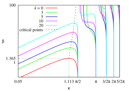
Figure 5: The electromagnetic interaction parameter $\beta$ versus the transverse wavenumber $\kappa$ for various longitudinal wavenumbers $k$.

There is another solution branch which explicitly describes interfacial wave instability. This genuinely unstable mode, which was missed by Lukyanov et al. (2001) and considered first by Morris & Davidson (2003), is defined by the complex frequencies $\omega$. In this case, the general solution of (59) decaying at $y\rightarrow\infty$ can be written as

$$\hat{\eta}(y)=\hat{\eta}_{0}e^{-y\kappa},$$ (65)

where $\kappa=\sqrt{k^{2}-\omega^{2}}$ represents the branch with positive real part. Substituting the solution above along with (63) into the boundary conditions (61), after a few rearrangements, we obtain the dispersion relation $\kappa(\kappa+k)+i\beta=0$, which yields

$$\kappa=\sqrt{\frac{k^{2}}{4}-i\beta}-\frac{k}{2}.$$

The respective frequency $\omega=\pm\sqrt{k^{2}-\kappa^{2}}$ then follows from the definition of $\kappa$ given below (65). The complexity of $\kappa$ for $\beta\not=0$ implies that one of the two frequencies has a positive imaginary part which, in turn, means that the respective mode is unstable at however small $\beta$. For $\beta/k^{2}=\varepsilon\ll 1$, which is close to the instability threshold and opposite to the limit of $\beta\gg 1$ producing the so-called edge waves (Morris & Davidson, 2003), we have $\kappa\approx-ik(\varepsilon+i\varepsilon^{2})$ and $\omega\approx\pm k(1+i\varepsilon^{3})$. These relations describe a slightly oblique wave with the transverse wavenumber $\beta/k\ll k$ which decays over the distance $\sim k^{3}/\beta^{2}$ from the wall and grows exponentially in time at the rate $\sim\beta^{3}/k^{5}$. Namely, in this model, the interface can be destabilised by an arbitrary weak electromagnetic effect which gives rise to a nearly transverse wave travelling along the wall.

It is instructive to contrast the instability in the semi-infinite model considered above with that in the slightly more realistic model of a finite-width channel. This model was first considered by Davidson & Lindsay (1998) and further studied in the context of hydromagnetic edge waves by Morris & Davidson (2003) and Molokov et al. (2011).

For a channel bounded by two lateral walls at $y=\pm 1$, the general solution of (59,60) can be written as

$$\hat{\eta}(y) = \hat{\eta}_{-}\sin(\kappa y)+\hat{\eta}_{+}\cos(\kappa y),$$ (66)

$$\hat{\phi}(y) = \hat{\phi}_{-}\sinh(ky)+\hat{\phi}_{+}\cosh(ky)+\omega^{-2}\hat{\eta}(y),$$ (67)

where $\kappa$ is the transverse wavenumber satisfying the dispersion relation of pure interfacial gravity waves

$$\omega^{2}=k^{2}+\kappa^{2}.$$ (68)

Figure 6: (a) Real $(\Re)$ and imaginary $(\Im)$ parts of the first three transverse wavenumbers $\kappa$, (b) the respective frequencies $\omega$ versus the electromagnetic interaction parameter $\beta$ for various longitudinal wavenumbers $k$ and (c) the critical $\beta$ and transverse wavenumbers $\kappa$ as functions of the longitudinal wavenumbers $k.$

Applying boundary conditions (61) at $y=\pm 1$, after a few rearrangements, we obtain

$$\beta(k,\kappa)=\pm\left(k^{2}+\kappa^{2}\right)\left(\frac{k}{\kappa}\left(\frac{k}{\kappa}+\frac{\tan\kappa}{\tanh k}-\frac{\tanh k}{\tan\kappa}\right)-1\right)^{-1/2},$$ (69)

which explicitly defines $\beta$ depending on the longitudinal and transverse wavenumbers $k$ and $\kappa.$ It is important to note that the respective eigenmode is a pure gravity wave as long as $\kappa$ is real. On the other hand, (69) implicitly defines the spectrum of admitted $\kappa$ values for given $k$ and $\beta$. For $\beta=0$, this equation reduces to $\sin 2\kappa=0$, which describes the standard wavenumber spectrum for a channel of dimensionless width equal to 2: $\kappa_{n}=n\pi/2,\,n=0,1,2,\ldots$. As seen in figure 5, where $\beta(k,\kappa)$ is plotted against $\kappa$ for various $k$, the increase of $\beta$ just modifies the spectrum of the wave modes admitted by the electromagnetic reflection condition (29). It is important to note that the eigenmodes remain pure gravity waves satisfying the dispersion relation (68) with real wavenumbers up to the point where two branches of $\kappa$ merge together. The absence of coupling between the gravity wave modes below the critical point is due to the effective reduction of the electromagnetic force to the boundary condition (29) which affects only the reflection but not the propagation of gravity waves. At the critical point, a complex conjugate pair of wavenumbers emerges, which means instability as the frequency becomes complex (see figure 6). As found by Morris & Davidson (2003), who use the reciprocal of $\beta$, this happens first at $\beta_{c}\approx 1.365$ when two purely longitudinal $(k=0)$ gravity wave modes with $\kappa_{c}=1.113$ merge.

Note that this critical mode is longitudinal and emerges at finite $\beta_{c}$, whereas the one predicted by the semi-infinite model is transverse and emerges at $\beta_{c}=0$. In the channel, the latter mode is recovered in the short-wave limit $k\gg 1$. For such waves, the marginal interaction parameter and the respective transverse wavenumber can be seen in figure 6(c) to scale as $\beta\sim k$ and $\kappa\sim 1$. The interaction parameter based on the wave length, which is the relevant horizontal length scale in this limit, then scales as $\widetilde{\beta}=\beta/k^{2}\sim k^{-1}\rightarrow 0$ so recovering the result of the semi-infinite model.

Appendix B Chebyshev collocation method

To solve the eigenvalue problem posed by (56) and (57) numerically we use a collocation method with the two-dimensional Chebyshev-Lobatto grid:

$$(x_{m},y_{n})=\frac{1}{2}\left(\sqrt{\alpha}\cos\frac{\pi m}{M+1},\frac{1}{\sqrt{\alpha}}\cos\frac{\pi n}{N+1}\right),(0,0)\leq(m,n)\leq(M+1,N+1),$$

on which the discretised solution $\{\hat{\eta},\hat{\phi}\}(x_{m},y_{n})=\{\boldsymbol{\mathrm{\eta}},\boldsymbol{\mathrm{\phi}}\}_{m,n}$ and its derivatives are sought. The latter are expressed in terms of the former by substituting the first and second derivatives with the differentiation matrices (Peyret, 2002, pp. 393–394). Requiring the equations to be satisfied at the inner collocation points $(1,1)\leq(m,n)\leq(M,N)$, we obtain a system of discrete equations which can be written as

$$-\lambda\boldsymbol{\mathrm{\eta}}_{0} = \boldsymbol{\mathsf{A}}_{0}\boldsymbol{\mathrm{\eta}}_{0}+\boldsymbol{\mathsf{A}}_{1}\boldsymbol{\mathrm{\eta}}_{1},$$ (70)

$$-\boldsymbol{\mathrm{\eta}}_{0} = \boldsymbol{\mathsf{A}}_{0}\boldsymbol{\mathrm{\phi}}_{0}+\boldsymbol{\mathsf{A}}_{1}\boldsymbol{\mathrm{\phi}}_{1},$$ (71)

where the subscripts $0$ and $1$ denote the parts of the solution at the inner and boundary collocation points respectively. The matrices $\boldsymbol{\mathsf{A}}_{0}$ and $\boldsymbol{\mathsf{A}}_{1}$ represent parts of the discretised Laplacian using the respective sets of points. The boundary conditions are applied the boundary points $m=0,M+1$ and $n=0,N+1$, which results in

$$\boldsymbol{\mathsf{B}}_{0}\boldsymbol{\mathrm{\eta}}_{0}+\boldsymbol{\mathsf{B}}_{1}\boldsymbol{\mathrm{\eta}}_{1} = \beta\boldsymbol{\mathsf{C}}\boldsymbol{\mathrm{\phi}}_{1},$$ (72)

$$\boldsymbol{\mathsf{B}}_{0}\boldsymbol{\mathrm{\phi}}_{0}+\boldsymbol{\mathsf{B}}_{1}\boldsymbol{\mathrm{\phi}}_{1} = \boldsymbol{\mathrm{0}},$$ (73)

where $\boldsymbol{\mathsf{B}}$ and $\boldsymbol{\mathsf{C}}$ are the discretised normal and tangential derivative operators at the boundary. The above system of discrete equations is reduced to a matrix eigenvalue problem as follows. First, (72) and (73) can solved for $\boldsymbol{\mathrm{\phi}}_{1}$ and $\boldsymbol{\mathrm{\eta}}_{1}$ in terms of $\boldsymbol{\mathrm{\phi}}_{0}$ and $\boldsymbol{\mathrm{\eta}}_{0}$ as

$$\boldsymbol{\mathrm{\phi}}_{1} = -\boldsymbol{\mathsf{B}}_{1}^{-1}\boldsymbol{\mathsf{B}}_{0}\boldsymbol{\mathrm{\phi}}_{0},$$ (74)

$$\boldsymbol{\mathrm{\eta}}_{1} = -\boldsymbol{\mathsf{B}}_{1}^{-1}\boldsymbol{\mathsf{B}}_{0}\boldsymbol{\mathrm{\eta}}_{0}+\beta\boldsymbol{\mathsf{B}}_{1}^{-1}\boldsymbol{\mathsf{C}}\boldsymbol{\mathrm{\phi}}_{1}.$$ (75)

Substituting (74) into (71), we have $\boldsymbol{\mathrm{\eta}}_{0}=-\boldsymbol{\mathsf{\widetilde{A}}}_{0}\boldsymbol{\mathrm{\phi}}_{0}$, where $\boldsymbol{\mathsf{\widetilde{A}}}_{0}=\boldsymbol{\mathsf{A}}_{0}-\boldsymbol{\mathsf{A}}_{1}\boldsymbol{\mathsf{B}}_{1}^{-1}\boldsymbol{\mathsf{B}}_{0}$. Combining this and (74) with (75) and (70), after a few rearrangements, we obtain the sought matrix eigenvalue problem

$$\lambda\boldsymbol{\mathrm{\phi}}_{0}=\left[-\boldsymbol{\mathsf{\widetilde{A}}}_{0}+\beta\boldsymbol{\mathsf{\widetilde{A}}}_{0}^{-1}\boldsymbol{\mathsf{A}}_{1}\boldsymbol{\mathsf{B}}_{1}^{-1}\boldsymbol{\mathsf{C}}\boldsymbol{\mathsf{B}}_{1}^{-1}\boldsymbol{\mathsf{B}}_{0}\right]\boldsymbol{\mathrm{\phi}}_{0},$$

which is solved using the standard DGEEV routine of LAPACK.

References

- Bojarevics (1998) Bojarevics, V. 1998 Nonlinear waves with electromagnetic interaction in aluminum electrolysis cells. In Prog. Fluid Flow Res.: Turbulence and Applied MHD (ed. H. Branover), , vol. 186, pp. 833–848. AIAA.
- Bojarevics & Pericleous (2006) Bojarevics, V. & Pericleous, K. 2006 Comparison of mhd models for aluminium reduction cells. In TMS Light Metals,, pp. 347–352.
- Bojarevics & Romerio (1994) Bojarevics, V. & Romerio, M.V. 1994 Long wave instability of liquid metal-electrolyte interface in aluminum electrolysis cells: a generalization of Sele’s criterion. Eur. J. Mech. B 13 (1), 33–56.
- Boyd (2013) Boyd, J. P. 2013 Chebyshev and Fourier Spectral Methods: Second Revised Edition. New York: Dover Publications.
- Davidson (1994) Davidson, P.A. 1994 An energy analysis of unstable, aluminim reduction cells. Eur. J. Mech. B 13 (1), 15–32.
- Davidson (2000) Davidson, P.A. 2000 Overview overcoming instabilities in aluminium reduction cells: a route to cheaper aluminium. Mater. Sci. Technol. 16 (5), 475–479.
- Davidson & Lindsay (1998) Davidson, P.A. & Lindsay, R.I. 1998 Stability of interfacial waves in aluminium reduction cells. J. Fluid Mech. 362, 273–295.
- Evans & Ziegler (2007) Evans, J. W. & Ziegler, D. P. 2007 The electrolytic production of aluminumn. In Encyclopedia of Electrochemistry (ed. A. J. Bard). Wiley.
- Gerbeau et al. (2006) Gerbeau, J.-F., Le Bris, C. & Lelièvre, T. 2006 Mathematical methods for the magnetohydrodynamics of liquid metals. Clarendon Press.
- Herreman et al. (2015) Herreman, W., Nore, C., Cappanera, L. & Guermond, J.-L. 2015 Tayler instability in liquid metal columns and liquid metal batteries. J. Fluid Mech. 771, 79–114.
- Herreman et al. (2019) Herreman, W., Nore, C., Guermond, J.-L., Cappanera, L., Weber, N. & Horstmann, G.M. 2019 Perturbation theory for metal pad roll instability in cylindrical reduction cells. J. Fluid Mech. 878, 598–646.
- Hertzberg et al. (2013) Hertzberg, T., Tørklep, K. & Øye, H.A. 2013 Viscosity of molten mixtures: Selecting and fitting models in a complex system. In Essential Readings in Light Metals, pp. 19–24. Wiley.
- Hinch (1991) Hinch, E. J. 1991 Perturbation Methods. Cambridge University Press.
- Horstmann et al. (2018) Horstmann, G. M., Weber, N. & Weier, T. 2018 Coupling and stability of interfacial waves in liquid metal batteries. J. Fluid Mech. 845, 1–35.
- Horstmann et al. (2019) Horstmann, G. M., Wylega, M. & Weier, T. 2019 Measurement of interfacial wave dynamics in orbitally shaken cylindrical containers using ultrasound pulse-echo techniques. Exp. Fluids 60 (4), 56.
- Kelley & Weier (2018) Kelley, D. H. & Weier, T. 2018 Fluid mechanics of liquid metal batteries. Appl. Mech. Rev. 70 (2), 020801.
- Kim et al. (2013) Kim, H., Boysen, D. A., Newhouse, J. M., Spatocco, B. L., Chung, B., Burke, P. J., Bradwell, D. J., Jiang, K., Tomaszowska, A. A., Wang, K., Wei, W., Ortiz, L. A., Barriga, S. A., Poizeau, S. M. & Sadoway, D. R. 2013 Liquid metal batteries: Past, present, and future. Chem. Rev. 113 (3), 2075–2099.
- Lukyanov et al. (2001) Lukyanov, A., El, G. & Molokov, S. 2001 Instability of MHD-modified interfacial gravity waves revisited. Phys. Lett. A 290 (3-4), 165–172.
- Molokov (2018) Molokov, S 2018 The nature of interfacial instabilities in liquid metal batteries in a vertical magnetic field. Europhys. Lett. 121 (4), 44001.
- Molokov et al. (2011) Molokov, S., El, G. & Lukyanov, A. 2011 Classification of instability modes in a model of aluminium reduction cells with a uniform magnetic field. Theor. Comput. Fluid Dyn. 25 (5), 261–279.
- Moreau & Ziegler (1988) Moreau, R. J & Ziegler, D. 1988 The Moreau-Evans hydrodynamic model applied to actual Hall-Héroult cells. Metall. Trans. B 19 (5), 737–744.
- Morris & Davidson (2003) Morris, S.J.S. & Davidson, P.A. 2003 Hydromagnetic edge waves and instability in reduction cells. J. Fluid Mech. 493, 121–130.
- Pedchenko et al. (2009) Pedchenko, A., Molokov, S., Priede, J., Lukyanov, A. & Thomas, P. J. 2009 Experimental model of the interfacial instability in aluminium reduction cells. Europhys. Lett. 88 (2), 24001.
- Peyret (2002) Peyret, R. 2002 Spectral methods for incompressible viscous flow. Springer.
- Priede (2017) Priede, J. 2017 Elementary model of internal electromagnetic pinch-type instability. J. Fluid Mech. 816, 705–718.
- Priede (2020) Priede, J. 2020 Self-contained two-layer shallow water theory of strong internal bores. arXiv:1806.06041 .
- Roberts (1967) Roberts, P. H. 1967 An Introduction to Magnetohydrodynamics. London: Longmans.
- Sele (1977) Sele, T. 1977 Instabilities of the metal surface in electrolytic alumina reduction cells. Metall. Trans. B 8 (3), 613–618.
- Sneyd (1985) Sneyd, A. D. 1985 Stability of fluid layers carrying a normal electric current. J. Fluid Mech. 156, 223–236.
- Sneyd & Wang (1994) Sneyd, A. D. & Wang, A 1994 Interfacial instability due to mhd mode coupling in aluminium reduction cells. J. Fluid Mech. 263, 343–360.
- Stefani et al. (2011) Stefani, F., Weier, T., Gundrum, Th. & Gerbeth, G. 2011 How to circumvent the size limitation of liquid metal batteries due to the Tayler instability. Energ. Convers. Manage. 52 (8), 2982–2986.
- Tucs et al. (2018a) Tucs, A., Bojarevics, V. & Pericleous, K. 2018a Magneto-hydrodynamic stability of a liquid metal battery in discharge. Europhys. Lett. 124 (2), 24001.
- Tucs et al. (2018b) Tucs, A., Bojarevics, V. & Pericleous, K. 2018b Magnetohydrodynamic stability of large scale liquid metal batteries. J. Fluid Mech. 852, 453–483.
- Urata (1985) Urata, N. 1985 Magnetics and metal pad instability. Light Metals pp. 581–589.
- Urata et al. (1976) Urata, N., Mori, K. & Ikeuchi, H. 1976 Behavior of bath and molten metal in aluminum electrolytic cell. J. Jpn. Inst. Light Met. 26 (11), 573–583.
- Weber et al. (2015) Weber, N., Galindo, V., Priede, J., Stefani, F. & Weier, T. 2015 The influence of current collectors on Tayler instability and electro-vortex flows in liquid metal batteries. Phys. Fluids 27 (1), 014103.
- Zikanov (2015) Zikanov, O. 2015 Metal pad instabilities in liquid metal batteries. Phys. Rev. E 92 (6), 063021.
- Zikanov et al. (2000) Zikanov, O., Thess, A., Davidson, P.A. & Ziegler, D.P. 2000 A new approach to numerical simulation of melt flows and interface instability in Hall-Heroult cells. Metal. Trans. B 31 (6), 1541–1550.