Rapidly Personalizing Mobile Health Treatment Policies
with Limited Data

Abstract

In mobile health (mHealth), reinforcement learning algorithms that adapt to one’s context without learning personalized policies might fail to distinguish between the needs of individuals. Yet the high amount of noise due to the in situ delivery of mHealth interventions can cripple the ability of an algorithm to learn when given access to only a single user’s data, making personalization challenging. We present IntelligentPooling, which learns personalized policies via an adaptive, principled use of other users’ data. We show that IntelligentPooling achieves an average of 26% lower regret than state-of-the-art across all generative models. Additionally, we inspect the behavior of this approach in a live clinical trial, demonstrating its ability to learn from even a small group of users.

1 Introduction

Mobile health (mHealth) interventions deliver treatments to users to support healthy behaviors. These interventions offer an opportunity for social impact in a diverse range of domains from substance abuse Rabbi et al. (2017), to disease management Hamine et al. (2015) to physical inactivity Consolvo et al. (2008). For example, to help users increase their physical activity, an mHealth application might send a walking suggestions at times and in locations when a user is likely to be able to pursue the suggestions. The promise of mHealth hinges on the ability to provide interventions at times when users need the support and are receptive to it Nahum-Shani et al. (2017). Consequently, in developing reinforcement learning (RL) algorithms for mHealth our goal is to be able to learn an optimal policy of when and how to intervene for a given user and context.

A significant challenge to learning an optimal policy is that there are often only a few opportunities per day to provide treatment. Furthermore, wearable sensors provide noisy estimates of critical metrics such as step counts Kaewkannate & Kim (2016). In mHealth settings, it is critical for an algorithm to learn quickly, in spite of noisy measurements and limited treatment data, as a poor policy can decrease user engagement and potentially increase the risk of a user leaving a trial or otherwise abandoning treatment. Standard reinforcement learning algorithms can learn poorly in these settings. Yet, demonstrations of the effectiveness of these approaches (especially through live clinical trials) are lacking, and essential to establishing their feasibility.

We present a personalized RL algorithm developed to meet the challenges of mHealth domains. Critically, we also evaluate its viability with a live clinical trial. To accelerate learning under the challenge of limited data we propose an approach that intelligently pools data from all users, according to a hierarchical Bayesian model, so as to more quickly learn an optimal policy for each. We use empirical Bayes to update the model hyper-parameters. This ensures that our approach is adaptive in that for each user the extent to which their own data (relative to data from the entire population) informs their policy is updated over time.

To inform the design of this clinical trial, we first conducted a smaller physical activity trial with sedentary individuals which we refer to as TrialOne. In TrialOne, contextual data was collected from each user’s fitness tracker and smartphone. We use this data to construct a simulation environment to evaluate our approach. By mirroring aspects of this trial we evaluate the algorithm in a challenging setting in which each user may experience the treatments a few times per day and in which the data is noisy. As similar settings exist beyond mHealth and there is a dearth of acceptable methods to contend with their challenges, we propose our approach as a general framework for principled pooling in RL algorithms. Our main contributions are:

• IntelligentPooling: A Thompson Sampling algorithm for rapid personalization in limited data settings. This algorithm employs empirical Bayes to adaptively adjust the degree to which policies are personalized to each user. We present an analysis of this adaptivity in Section 3.4 showing that IntelligentPooling learns to personalize to a user as a function of the observed variance in the treatment effect both between and within users.

• An empirical evaluation of our approach in a simulation environment constructed from mHealth data. IntelligentPooling not only achieves 26% lower regret than state-of-the-art, it also is better able to adapt to the degree of heterogeneity present in a population.

• Evidence of the practicality of our approach from a live clinical trial. A driving motivation of this work is to provide a reinforcement learning algorithm that can face the challenges of limited data in noisy online settings. We demonstrate that IntelligentPooling can be executed in a real-time online environment.

2 Related Work

In mHealth several algorithms have been proposed for learning treatment policies. These have typically followed two main paradigms. The first is learning a treatment policy for each user separately, such as Rabbi et al. (2015), Jaimes et al. (2016), and Forman et al. (2018). This approach makes sense when users are highly heterogeneous, that is, their optimal policies differ greatly one from another. However, this situation can present challenges for learning the policy when data is scarce and/or noisy, as in our motivating example of encouraging activity in an mHealth study where only a few decision time-points occur each day. The second paradigm is learning one treatment policy for all users both in bandit algorithms Bouneffouf et al. (2012); Paredes et al. (2014); Yom-Tov et al. (2017), and in full reinforcement learning algorithms Clarke et al. (2017); Zhou et al. (2018). This second approach can potentially learn quickly but may result in poor outcomes if the optimal policies differ much between users. In this work we demonstrate that a pooled approach has advantages over each of these paradigms. When users are heterogenous, our method achieves lower regret than batch approaches, and more quickly than personalized approaches. When users are homogenous our method performs as well as the batch approach.

Our proposed algorithm uses a mixed (random) effects Gaussian process (GP) model as part of a Thompson Sampling algorithm. While Gaussian process models have been used for multi-armed bandits Chowdhury & Gopalan (2017); Brochu et al. (2010); Srinivas et al. (2009); Desautels et al. (2014); Wang et al. (2016); Djolonga et al. (2013); Bogunovic et al. (2016) , and for contextual bandits Li et al. (2010); Krause & Ong (2011), there is no work establishing their success in a setting with the challenges posed by mHealth. Furthermore, though our use of a mixed-effects GP resembles that of Shi et al. (2012); Luo et al. (2018) we consider a mixed-effects model in the context of RL rather than the previously considered prediction setting.

While we propose a bandit approach that pools across users in a structured manner, others have proposed pooling in other ways: Deshmukh et al. (2017) pool data from different arms of a single bandit, and Li and Kar (2015) use context-sensitive clustering to produce aggregate reward estimates for the UCB bandit algorithm. More relevant to this work are multi-task GPs, e.g. Lawrence & Platt (2004); Bonilla et al. (2008); Wang & Khardon (2012), however these have been proposed in the prediction as opposed to the RL setting. The Gang of Bandits Cesa-Bianchi et al. (2013); Vaswani et al. (2017) approach has been shown to be successful when there is prior knowledge on the similarities between users. For example, a social network graph might provide a mechanism for pooling. In contrast, our approach does not require prior knowledge of relationships between users and we adaptively update the degree of personalization.

3 Our Approach

We present an approach for learning personalized treatment policies in mHealth settings, where a policy takes the user’s current context as input and outputs a treatment. For example, context might include current location/weather while a treatment might be a physical activity message. Here, our goal is to learn such policies within a clinical trial in which users enroll incrementally. During the trial the developed algorithm will learn a policy for each user based on the user’s prior data as well as data from current and past users.

3.1 Problem setting

Let $i\in[N]=\{1,\dots,N\}$ be the user index. For each user, we use $k\in\{1,2,\dots\}$ to index decision times, i.e., times at which a treatment could be provided. Denote by $S_{i,k}$ the contextual features at the $k$-th decision time of user $i$, such as location. Let $A_{i,k}$ be the selected treatment. For simplicity, we consider binary treatment $\mathcal{A}=\{0,1\}$. Recall that users enter the trial in staggered fashion. We denote by $t_{i,k}$ the calendar time of user $i$’s $k$-th decision time.

Our objective is to learn individual treatment policies for $N$ individuals; we treat this as $N$ contextual bandit problems. We note that maintaining $N$ separate problems is important in settings such as ours where the true context is only sparsely observed and there is significant unobserved heterogeneity among different users. Section 3.2 reviews two approaches for using Thompson Sampling Agrawal & Goyal (2012) and Section 3.3 presents our approach for learning the treatment policy for any specific user.

3.2 Two Thompson Sampling instantiations

First consider learning the treatment policy separately per person. We refer to this approach as Person-Specific. At each decision time $k$, we would like to select a treatment $A_{i,k}\in\{0,1\}$ based on the context $S_{i,k}$. We model the reward $R_{i,k}$ by a Bayesian linear regression model: for user $i$ and time $k$

$${R_{i,k}=\phi(S_{i,k},A_{i,k})^{\top}\theta_{i}+\epsilon_{i,k}}$$ (1)

where $\phi(s,a)$ is a feature vector of context and treatment variables that are predictive of rewards (e.g. those described in Section 4.2), $\theta_{i}$ is a parameter vector which we will learn, and $\epsilon_{i,k}\sim\mathbf{N}(0,\sigma_{\epsilon}^{2})$ is the error term. The parameters $\{\theta_{i}\}$ are assumed independent across users and to follow a common prior distribution $\theta_{i}\sim\mathbf{N}(\mu_{\theta},\Sigma_{\theta})$.

Now at any decision time $k$, given the user’s history so far $\mathcal{D}_{i,k}=\{(S_{i,o},A_{i,o},R_{i,o}):o\leq k-1\}$ and the current context $S_{i,k}$, we use Thompson Sampling to select the treatment. That is, select treatment $A_{i,k}=1$ with probability $\pi_{i,k}$:

$$\pi_{i,k}=\textrm{Pr}\{\phi(S_{i,k},1)^{\top}\tilde{\theta}_{i,k}>\phi(S_{i,k},0)^{\top}\tilde{\theta}_{i,k}\}$$ (2)

where $\tilde{\theta}_{i,k}$ follows the posterior distribution of $\theta_{i}$ given $\mathcal{D}_{i,k}$. We note that the posterior distribution of $\theta_{i}$ is formed based on the user’s own data.

In many mHealth applications, the combination of noisy data and low numbers of decision point observations per day means that learning the treatment policy separately for each user can cause slow policy improvement. This motivates leveraging data collected from other users to improve learning the optimal treatment policy for each user. A straightforward approach is to learn a common bandit model for all users. In this setting, there are no individual-level parameters. The model is a single Bayesian regression model:

$$R_{i,k}=\phi(S_{i,k},A_{i,k})^{T}\theta+\epsilon_{i,k}.$$ (3)

Note that $\theta$ does not vary by user. We then use the posterior distribution of the parameter $\theta$ to sample treatments for each user. This approach, which we refer to as Complete, may suffer from high bias when there is significant heterogeneity among users. This motivates our proposed method.

3.3 Intelligent pooling across bandit problems

In our approach, which we call IntelligentPooling, we pool information across users in an adaptive way, i.e., when there is strong homogeneity observed in the current data, the method will pool more from others than when there is strong heterogeneity.

Bayesian random effects model

Consider the Bayesian linear regression model (1). Instead of considering the $\theta_{i}$s as separate parameters to be estimated, we impose a random-effects structure Raudenbush & Bryk (2002); Laird et al. (1982) on $\theta_{i}$:

$${\theta_{i}=\theta_{pop}+u_{i}}$$ (4)

$\theta_{pop}$ is a population-level parameter and $u_{i}$ represents the person-specific deviation from $\theta_{pop}$ for user $i$.

We use the following prior for this model: (1) $\theta_{pop}$ has prior mean $\mu_{\theta}$ and variance $\Sigma_{\theta}$, (2) $u_{i}$ has mean $\mathbf{0}$ and covariance $\Sigma_{u}$, and (3) $u_{i}\mathchoice{\mathrel{\hbox to0.0pt{$\displaystyle\perp$\hss}\mkern 2.0mu{\displaystyle\perp}}}{\mathrel{\hbox to0.0pt{$\textstyle\perp$\hss}\mkern 2.0mu{\textstyle\perp}}}{\mathrel{\hbox to0.0pt{$\scriptstyle\perp$\hss}\mkern 2.0mu{\scriptstyle\perp}}}{\mathrel{\hbox to0.0pt{$\scriptscriptstyle\perp$\hss}\mkern 2.0mu{\scriptscriptstyle\perp}}}u_{j}$ for $i\neq j$ and $\theta_{pop}\mathchoice{\mathrel{\hbox to0.0pt{$\displaystyle\perp$\hss}\mkern 2.0mu{\displaystyle\perp}}}{\mathrel{\hbox to0.0pt{$\textstyle\perp$\hss}\mkern 2.0mu{\textstyle\perp}}}{\mathrel{\hbox to0.0pt{$\scriptstyle\perp$\hss}\mkern 2.0mu{\scriptstyle\perp}}}{\mathrel{\hbox to0.0pt{$\scriptscriptstyle\perp$\hss}\mkern 2.0mu{\scriptscriptstyle\perp}}}\{u_{i}\}$ .

The variables $\mu_{\theta},\Sigma_{\theta}$ as well as the variance of the person-specific effect $\Sigma_{u}$, and the residual variance $\sigma_{\epsilon}^{2}$ are hyper-parameters. In the prior (Eqn. 4), we assume the person-specific effect on each element of the parameters $\theta$. In practice, one can use domain knowledge to specify which of the parameters should have the person-specific deviations; this will be the case in the experiments below.

We denote by $\mathcal{T}$ the set of times that the posterior distribution is updated. Specifically, let $T\in\mathcal{T}$ be an updating time and $\mathcal{U}_{T}\subseteq[N]$ be the set of users that are currently in or have finished the trial. The history available at time $T$ is $\mathcal{D}_{T}=\{(S_{i,k},A_{i,k},R_{i,k},i):i\in\mathcal{U}_{T},t_{i,k}\leq T\}$. Suppose the number of tuples in $\mathcal{D}_{T}$ is $n_{T}$.

The posterior distribution of each $\theta_{i}$ is Gaussian with mean and variance determined by a kernel function $K$ induced by the random effects model (Eqns. 1, 4): for any two tuples in $\mathcal{D}_{T}$, e.g., $x_{l}=(S^{(l)},A^{(l)},R^{(l)},i_{l}),l=1,2$

$$K(x_{1},x_{2}) =\phi_{1}^{\top}(\Sigma_{\theta}+\mathbbm{1}_{\{i_{1}=i_{2}\}}\Sigma_{u})\phi_{2}$$ (5)

where $\phi_{l}=\phi(S^{(l)},A^{(l)})$. Note that the above kernel depends on $\Sigma_{\theta}$ and $\Sigma_{u}$. The kernel matrix $\mathbf{K}_{n_{T}}$ is of size $n_{T}\times n_{T}$ and each element is the kernel value between two tuples in $\mathcal{D}_{T}$. The posterior mean and variance of $\theta_{i}$ given $\mathcal{D}_{T}$ can be calculated by

$$\begin{split}\mu_{i,T}&=\mu_{\theta}+M_{i}^{\top}(\mathbf{K}_{n_{T}}+\sigma_{\epsilon}^{2}I_{T})^{-1}\tilde{R}_{n_{T}}\\ \Sigma_{i,T}&=\Sigma_{\theta}+\Sigma_{u}-M_{i}^{\top}(\mathbf{K}_{n_{T}}+\sigma_{\epsilon}^{2}I_{n_{T}})^{-1}M_{i}\end{split}$$ (6)

where $\tilde{R}_{n_{T}}$ is the vector of the rewards centered by the prior means, i.e., each element corresponds to a tuple $(S,A,R,j,h)$ in $\mathcal{D}_{T}$ given by $R-\phi(S,A)^{\top}\mu_{\theta}$, and $M_{i}$ is a matrix of size $n_{T}$ by $p$, with each row corresponding to a tuple $(S,A,R,j)$ in $\mathcal{D}_{T}$ given by $\phi(S,A)^{\top}(\Sigma_{\theta}+\mathbbm{1}_{\{j=i\}}\Sigma_{u})$.

Treatment selection

To select a treatment for user $i$ at the $k$-th decision time, we use the posterior distribution of $\theta_{i}$ formed at the most recent update time $T$. That is, for the context $S_{i,k}$ of user $i$ at the $k$-th decision time, IntelligentPooling selects the treatment $A_{i,k}=1$ with probability

$$\pi_{i,k}=\textrm{Pr}\{\phi(S_{i,k},1)^{\top}\tilde{\theta}_{i,T}>\phi(S_{i,k},0)^{\top}\tilde{\theta}_{i,T}\}$$ (7)

where $\tilde{\theta}_{i,k}\sim\mathbf{N}(\mu_{i,T},\Sigma_{i,T})$.

Updating hyper-parameters

Thus far the degree of pooling across users has been determined by the choice of the hyper-parameters. While the prior mean $\mu_{\theta}$ and variance $\Sigma_{\theta}$ of the population parameter $\theta_{pop}$ can be set according to previous data or domain knowledge, it is difficult to pre-tune the variance components of the random effects. Also the influence of the prior mean and variance on the Thompson Sampling algorithm decreases as data accrues and is used by the algorithm. However the influence of the variance components for the random effects on the degree of pooling persists even with increasing user data. Thus at the update times, we use an empirical Bayes Carlin & Louis (2010) approach to update $\lambda=(\Sigma_{u},\sigma_{\epsilon}^{2})$. The updated values maximize the marginal log-likelihood of the observed reward, marginalized over the population parameters $\theta_{pop}$ and the random effects. At every update time, $T$, we set the hyper-parameters as $\hat{\lambda}=\operatornamewithlimits{argmax}\limits l(\lambda|\mathcal{D}_{T})$, the maximizer of the marginal likelihood $l(\lambda|\mathcal{D}_{T})$:

$$\begin{split}&l(\lambda|\mathcal{D}_{T})=-\frac{1}{2}[\tilde{R}_{n_{T}}^{\top}(\mathbf{K}_{n_{T}}(\lambda)+\sigma_{\epsilon}^{2}I_{n_{T}})^{-1}\tilde{R}_{n_{T}}\\ &\qquad+\log\det(\mathbf{K}_{n_{T}}(\lambda)+\sigma_{\epsilon}^{2}I_{n_{T}})+n_{T}\log(2\pi)]\end{split}$$ (8)

where $\mathbf{K}_{n_{T}}(\lambda)$ is the kernel matrix as a function of parameters $\lambda=(\Sigma_{u},\sigma_{\epsilon}^{2})$. IntelligentPooling is outlined in Algorithm 1.

Algorithm 1 Thompson Sampling with Intelligent Pooling (IntelligentPooling)

1:  Initialize the posterior distribution $\{post(i)\}$ by the prior

2:  for $t\in[0,T]$ do

3:    Receive user index $i$ and decision time index $k$

4:    Collect state variable $S$

5:    Obtain posterior distribution $post(i)$ of $\theta_{i}$

6:    Calculate randomization probability $\pi$ in Eqn 7

7:    Sample treatment $A\sim\operatorname{Bern}\left({\pi}\right)$

8:    Collect reward $R$

9:    $\mathcal{D}\leftarrow\mathcal{D}\cup\{S,A,R,i\}$

10:    if $t\in\mathcal{T}$ then

11:       Update the hyper-parameters: $\lambda=\operatornamewithlimits{argmax}\limits l(\lambda|\mathcal{D})$ in Eqn 8

12:       Update the posterior $post(\cdot)=post(\cdot|\mathcal{D},\lambda)$ by Eqns 6

13:    end if

14:  end for

3.4 Impact of hyper-parameters

Ideally, IntelligentPooling should learn to pool adaptively based on the users’ heterogeneity. That is, the person-specific random effect should outweigh the population term if users are highly heterogenous. If users are highly homoegenous, the person-specific random effect should be outweighed by the population term. The amount of pooling is controlled by the hyper-parameters, e.g., the variance components of the random effects.

To gain intuition, we consider a simple setting where the feature vector $\phi$ in the reward model (Eqn. 1) is one-dimensional (i.e., $p=1$) and there are only two users (i.e., $i=1,2$). Denote the prior distributions of population parameter $\theta_{pop}$ by $\mathbf{N}(0,\sigma_{\theta}^{2})$ and the random effect $u_{i}$ by $\mathbf{N}(0,\sigma_{u}^{2})$. Below we investigate how the hyper-parameters (e.g., $\sigma_{u}^{2}$ in this simple case), impact the posterior distribution.

Let $k_{i}$ be the index of decision time of user $i$ at the updating time $T$. In this simple setting, the posterior mean of $\theta_{1}$ can be calculated explicitly by

$$\mu_{1}=\frac{[\delta\gamma+(1-\gamma^{2})S_{2}]Y_{1}+\delta\gamma^{2}Y_{2}}{(1-\gamma^{2})S_{1}S_{2}+\delta\gamma(S_{1}+S_{2})+(\delta\gamma)^{2}}$$

where for $i=1,2$, $S_{i}=\sum_{k=1}^{k_{i}}\phi(A_{i,k},S_{i,k})^{2}$, $Y_{i}=\sum_{k=1}^{k_{i}}\phi(A_{i,k},S_{i,k})R_{i,k}$, $\gamma=\sigma_{\theta}^{2}/(\sigma_{\theta}^{2}+\sigma_{u}^{2})$ and $\delta=\sigma_{\epsilon}^{2}/\sigma_{\theta}^{2}$. Similarly, the posterior mean of $\theta_{2}$ is given by

$$\mu_{2}=\frac{[\delta\gamma+(1-\gamma^{2})S_{1}]Y_{2}+\delta\gamma^{2}Y_{1}}{(1-\gamma^{2})S_{1}S_{2}+\delta\gamma(S_{1}+S_{2})+(\delta\gamma)^{2}}$$

When $\sigma_{u}^{2}\rightarrow 0$ (i.e., the variance of person-specific effect goes to 0), we have $\gamma\rightarrow 1$ and both posterior means

$$\mu_{1},\mu_{2}\rightarrow\frac{Y_{1}+Y_{2}}{S_{1}+S_{2}+\delta},$$

which is the posterior mean under the model Complete (Eqn 3) using prior $\mathbf{N}(0,\sigma_{\theta}^{2})$. On the other hand, when $\sigma_{u}^{2}\rightarrow\infty$, we have $\gamma\rightarrow 0$ and

$$\mu_{1}\rightarrow\frac{Y_{1}}{S_{1}},~{}\mu_{2}\rightarrow\frac{Y_{2}}{S_{2}}$$

where correspond to the person-specific estimation of $\theta_{1}$ and $\theta_{2}$ under the model Person-Specific (Eqn 1) using a non-informative prior. Fig. 1 illustrates that when $\gamma$ goes from 0 to $1$, the posterior mean of $\theta_{i}$ smoothly transits from the population estimates to the person-specific estimates.

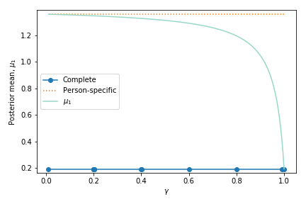
Figure 1: The posterior mean of $\theta_{i}$, $\mu_{1}$. As the variance of random effect $\sigma_{u}^{2}$ decreases, $\gamma$ increases and the posterior mean approaches the population-informed estimation (Complete) and departs from the person-specific estimation (Person-specific).

4 Experiments

This work was conducted to prepare for deployment of our algorithm in a live trial. Thus, to evaluate our approach we construct a simulation environment from a precursor trial, TrialOne. This simulation allows us to evaluate the proposed algorithm under various settings that may arise in implementation. For example, heterogeneity in the observed rewards may be due to unknown subgroups across which users differ in their response to treatment. Alternatively, this heterogeneity may vary across users in a more continuous manner. We consider both scenarios in simulated trials. In Sections 4.1-4.3 we evaluate the performance of IntelligentPooling against baselines and state-of-the-art. Having established its feasibility through a simulated environment, in Section 5 we evaluate a pilot deployment of IntelligentPooling in a clinical setting.

4.1 Simulation environment

TrialOne data is used to construct all features within the environment, and to guide choices such as how often to update the feature values. $S_{i,k}$ and $R_{i,k}$ denote the context features and reward of user $i$ at time $k$, respectively. The reward is the log step counts in the thirty minutes immediately following a decision time. Selecting treatment one corresponds to sending an activity-suggestion message which requires several minutes of a user’s time. Alternatively, selecting treatment zero corresponds to sending a less burden-some message suggesting a very brief (30 second) activity.

Fig. 2 describes the simulation while Table 1 describes context features and rewards. Each context feature in Table 1 was constructed from TrialOne data. For example, we found that in TrialOne data splitting participants’ preceding activity levels into the two categories of high or low best explained the reward.

The temperature and location are updated throughout a simulated day according to probabilistic transition functions constructed from TrialOne. The step counts for a simulated user are generated from participants in TrialOne as follows. We construct a one-hot encoding containing the group-ID of a participant, the time of day, the day of the week, the temperature, the preceding activity level, and the location. Then for each possible realization of the one-hot encoding we calculate the empirical mean and empirical standard deviation of all step counts observed in TrialOne.

Let $i$ denote the $i^{th}$ simulated user and $k$ denote a decision time. This simulated user’s context is encoded via the same one-hot encoding to produce $h(S_{i,k})$. The corresponding empirical mean and empirical standard deviation from TrialOne form $\mu_{h(S_{i,k})}$ $\sigma_{h(S_{i,k})}$ respectively. At non-decision times step counts are generated according to

$$R_{i,k}=\mathbf{N}(\mu_{h(S_{i,k})},\sigma^{2}_{h(S_{i,k})}).$$ (9)

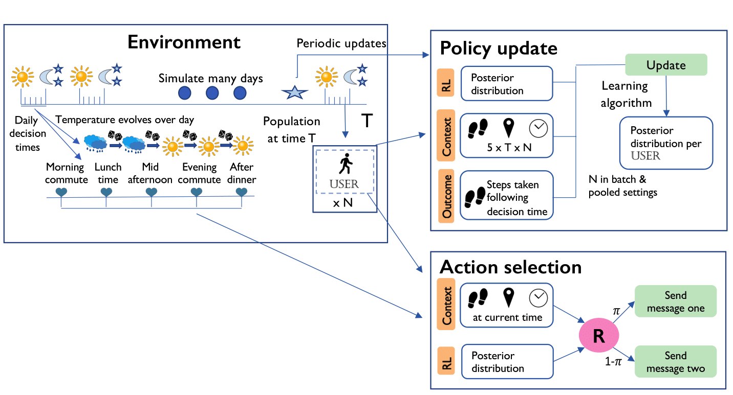
Figure 2: Contextual features for a simulated User are composed of both general environmental features (such as time of day) and individual features (such as location). At decision times a simulated user receives a message determined by the current treatment policy. Periodically this policy is updated according to a learning algorithm which outputs a new posterior distribution for each User.

State Features
Name	Value	User Specific
Time of day	Morning(0) 9:00 and 15:00 Afternoon(1) 15:00 and 21:00 Night(2) 21:00 and 9:00	No
Day of the week	Weekday(0) or Weekend(1)	No
Temperature	Cold(0) or Hot(1)	No
Preceding activity level	Low(0) or High(1)	Yes
Location	Other(0) or Home/work(1)	Yes
Intercept	1	Yes
Reward
Step count	Continuous on log scale	Yes

Table 1: The value used in encoding each feature is shown in parentheses. For example cold(0) indicates that cold is coded as a 0 wherever this feature is used.

Heterogeneity This model, which we denote Heterogeneity, allows us to compare the performance of the approaches under different levels of population heterogeneity. The step count after a decision time is a modification of Eqn. 9 to reflect the interaction between context and treatment on the reward and heterogeniety in treatment effect. Let $f(S_{i,k})\subseteq h(S_{i,k})$. Let $\beta$ be a vector of coefficients of $f(S_{i,k})$ which weigh the relative contributions of the entries of $f(S_{i,k})$ that interact with treatment on the reward. The magnitude of the entries of $\beta$ are set using TrialOne. Step counts ($R_{i,k}$) are generated as

$$R_{i,k}=\mathbf{N}(\mu_{h(S_{i,k})},\sigma^{2}_{h(S_{i,k})})+A_{i,k}(f(S_{i,k})^{T}\beta_{i}+Z_{i}).$$ (10)

The inclusion of $Z_{i}$ will allow us to evaluate the relative performance of each approach under different levels of population heterogeneity. Let $\beta^{l}_{i}$ be the coefficient of the location term for the $i^{th}$ user. We consider three scenarios (shown in Table 2) to generate $Z_{i}$, the person-specific effect, and $\beta^{l}_{i}$ the location-dependent person-specific effect. The performance of each algorithm under each scenario will be analyzed in Section 4.3. In the smooth scenario, $\sigma$ is equal to the standard deviation of the observed treatment effects $[f(S_{i,k})^{\top}\beta\ :\ S_{i,k}\in\textsc{TrialOne}{}]$ and $\beta^{l}_{i}$ is set to 0.1.

In the bi-modal scenario each simulated user is assigned a base-activity level: low-activity users or high-activity users (these two groups were constructed from analyses of TrialOne using non-parametric clustering). When a simulated user joins the trial they are placed into either group one or two with equal probability. The values of $z_{1},\beta^{l}_{1}$ and $z_{2},\beta^{l}_{2}$ are set so that for all users in group 1, it is optimal to send a treatment  75% of the time while for all users in group 2 it is optimal to send a treatment  25% of the time. Group membership is not known to any of the algorithms.

Homogeneous	Bi-modal	Smooth
$Z^{i}=0$ $\beta^{l}_{i}$=0	$Z_{i},\beta^{l}_{i}=\begin{cases}z_{1},\beta^{l}_{1}&\text{if}\ i\in\text{group one}\\ z_{2},\beta^{l}_{2}&\text{if}\ i\in\text{group two}\end{cases}$	$Z_{i}\sim\mathcal{N}(0,\sigma^{2})$ $\beta^{l}_{i}\sim\mathcal{N}(0,\sigma_{l}^{2})$

Table 2: Settings for Z in three cases of homogeneous, bimodal and smoothly varying populations.

When a simulated user is at a decision time the user will receive a treatment according to whichever RL policy is being run through the simulation.

4.2 Simulation implementation details

In Section 3 we introduced the feature vector $\phi$, recall that $\phi$ is the vector $\phi(S_{i,k},A_{i,k})\in\mathbb{R}^{p}$ used in the model for the reward. The features in the reward model for all algorithms considered here are,

$$\begin{split}\phi(S_{i,k},A_{i,k})^{T}=&\big{(}g(S_{i,k},A_{i,k})^{T},\pi_{i,k}f(S_{i,k})^{T},\\ &\qquad(A_{i,k}-\pi_{i,k})f(S_{i,k})^{T}\big{)}\end{split}$$ (11)

where $g(S_{i,k})$ is a subset of $h(S_{i,k})$, containing: an intercept term (equal to $1$), time of day, day of the week, preceding activity level, and location and $f(S_{i,k})=g(S_{i,k})$. Recall that the bandit algorithms produce $\pi_{i,k}$ which is the probability that $A_{i,k}=1$.

The inclusion of the term $\small{(A_{i,k}-\pi_{i,k})f(S_{i,k})}$ is motivated by Liao et al. (2016); Boruvka et al. (2018); Greenewald et al. (2017), who demonstrated that action-centering can protect against mis-specification in the baseline effect (e.g., the expected reward under the action 0). In TrialOne we observed that users varied in their overall responsivity and that a user’s location was related to their responsivity. In the simulation, we assume the person-specific random effect on four parameters in the reward model (i.e., the coefficients of terms in $g$ and $f$ involving the intercept and location).

Finally, we constrain the randomization probability to be within [0.1, 0.8] to ensure continual learning. The update time for the hyper-parameters is set to be every 7 days. All approaches are implemented in Python and we implement GP regression with the software package GPytorch Gardner et al. (2018).

4.3 Simulation results

In this section, we present an empirical analysis of our algorithm (IntelligentPooling), comparing to two standard methods Complete and Person-Specific, which are outlined in Section 3.2. Recall that IntelligentPooling includes person-specific random effects, as described in Eqn. 4. In Person-Specific, all users are assumed to be different and there is no pooling of data and in Complete, we treat all users the same and learn one set of parameters across the entire population.

Additionally, to assess IntelligentPooling’s ability to pool across users we compare our approach to Gang of Bandits Cesa-Bianchi et al. (2013), which we refer to as GangOB. As this model requires a relational graph between users, we construct a graph using the generative model Heterogeneity which connects users according to each of the three settings: homogenous, bi-modal and smooth. For example, with knowledge of the generative model users can be connected to other users as a function of their $Z_{i}$ terms. As we will not have true access to the underlying generative model in a real-life setting we distort the true graph to reflect this incomplete knowledge. That is we add ties to dissimilar users at 50% of the strength of the ties between similar users.

Let $a^{*}_{i,k}=\mathbbm{1}_{\{f(S_{i,k})^{T}\beta_{i}^{*}+Z_{i}\geq 0\}}$ be the optimal action for user $i$ at time $k$. We calculate the regret as

$$\text{regret}_{i,k}=|f(S_{i,k})^{T}\beta_{i}^{*}+Z_{i}|\mathbbm{1}_{\{a^{*}_{i,k}\neq A_{i,k}\}}$$ (12)

where $\beta^{*}_{i}$ is the optimal $\beta$ for the $i^{th}$ user.

In these simulations each trial has 32 users. Each user remains in the trial for 10 weeks and the entire length of the trial is 15 weeks, where the last cohort joins in week six. The number of users who join each week is a function of the recruitment rate observed in TrialOne. In all settings we run 50 simulated trials.

First, Fig. 3 provides the regret averaged across all users across 50 simulated trials where the reward distribution follows the generative model Heterogeneity. Though users join the trial in a staggered fashion, so that in the first week of the trial only a few users are active, the horizontal axis in Fig. 3 is the average regret over all users in their nth week in the trial, e.g. in their first week, their second week, etc. In the bi-modal setting there are two groups, where all users in group one have a positive response to treatment on average, while the users in group two have a negative response to treatment. An optimal policy would learn to not send interventions to users in the first group, and to send them to users in the second. To evaluate each algorithm’s ability to learn this distinction we show the percentage of time each group received a message in Table 3.

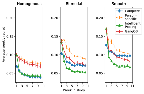
Figure 3: Heterogeneity generative model Regret averaged across all users for each week in the trial, i.e. average regret of all users in their first week of the trial.

	Group one optimal policy = send	Group two optimal policy = don’t send
Complete	0.49	0.46
Person- Specific	0.65	0.49
GangOB	0.57	0.35
Intelligent- Pooling	0.59	0.36

Table 3: Average fraction of times treatment was sent (action=1), over 50 simulations (bi-modal generative model $Z^{b}$).

The relative performance of the approaches depends on the heterogeneity of the population. When the population is very homogenous Complete excels, while its performance suffers as heterogeneity increases. Person-Specific is able to personalize; as shown by Table 3, it can differentiate between individuals. However, it learns slowly and can only approach the performance of Complete in the smooth setting of Heterogeneity where users differ the most in their response to treatment. Both IntelligentPooling and GangOB are more adaptive than either Complete or Person-Specific. GangOB consistently outperforms Person-Specific and achieves lower regret than Complete in some settings. In the homeogenous setting we see that GangOB can utilize social information more effectively than Person-Specific does while in the smooth setting it can adapt to individual differences more effectively than Complete. Yet, IntelligentPooling demonstrates stronger and swifter adaptability than does GangOB, consistently achieving lower regret at quicker rates. Finally, the algorithms differ in their suitability for real-world applications, especially when data is limited. GangOB requires reliable values for hyper-parameters and can depend on fixed knowledge about relationships between users. IntelligentPooling can learn how to pool between individuals over time and without prior knowledge.

5 IntelligentPooling Pilot

The simulated experiments provide insights into the potential of this approach for a live deployment. As we see reasonable performance in the simulated setting, we now discuss an initial pilot deployment of IntelligentPooling in a physical activity clinical trial setting, which we refer to as Pilot. In Pilot, following an initial ten users in the clinical trial IntelligentPooling is deployed for each of the subsequent ten users. At each decision time for these subsequent ten users, Algorithm 1 uses all data up to that decision time (i.e. from the initial ten users as well as from the subsequent ten users).

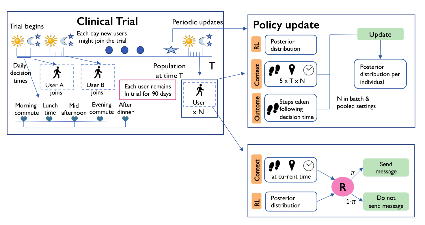
Figure 4: Setup of Pilot. Here we see that users can receive treatments up to five times a day and that each user remains in the trial for 90 days. Users enter the trial asynchronously.

Fig. 4 provides details of this pilot study. We use the Bayesian Thompson Sampling model shown in Section 4.2. The features used in the trial are shown in in Table 4. The feature engagement represents the extent to which a user engages with the mHealth application measured as a function of how many screen views are made within the application. The feature dosage represents the extent to which a user has received interventions. This feature is designed to increase with exposure to intervention but can decline when a treatment is skipped. Thus, if a user did not receive treatment for a sufficient period of time their dosage could be low. We provide a full description of these features in Section 3 of the supplement. As Pilot only includes a small number of users, we deploy a simple model with two person-specific random effects on the intercept term in $g$ and $f$ (Eqn. 11).

State Features
Name	Value	User Specific	Included in $f$
Temperature	Continuous	Yes (based on location)	No
Preceding activity level	Continuous	Yes	No
Variation in preceding activity level	Continuous	Yes	Yes
Engagement with mobile application	Continuous	Yes	Yes
Dosage	Continuous	Yes	Yes
Location	Other(0) or Home/work(1)	Yes	Yes
Intercept	1	Yes	Yes
Reward
Step count	Continuous on log scale	Yes	NA

Table 4: State feature descriptions for Pilot.

Personalization in Pilot By comparing how the decisions to treat under IntelligentPooling differ from those under Complete, we provide preliminary evidence that IntelligentPooling personalizes to users. Fig. 5 displays the posterior mean of the coefficient of the $A_{i,k}-\pi_{i,k}$ term in $f$. This coefficient represents the overall effect of treatment on user $i$. During the prior 7 days the user has not experienced much variation in activity at this time and the user’s engagement is low. Note that the treatment appears to have a positive effect on User B in this context whereas on User A there is little evidence of a positive effect. If Complete had been used to determine treatment, user A might have been over-treated.

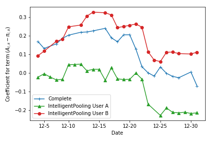
Figure 5: Posterior mean of the coefficient of $(A_{i,k}-\pi_{i,k})$ in Eqn. 11 for users A and B.

For each user we calculated the difference in treatment probabilities between IntelligentPooling and Complete. We see a weak linear trend with time (Fig. 6), that is, as more data accumulates the difference between treatment probabilities under Complete and IntelligentPooling grows, with a Pearson correlation coefficient of .56 ($p<.1$). This is a signal that personalization strengthens as a user provides more data.

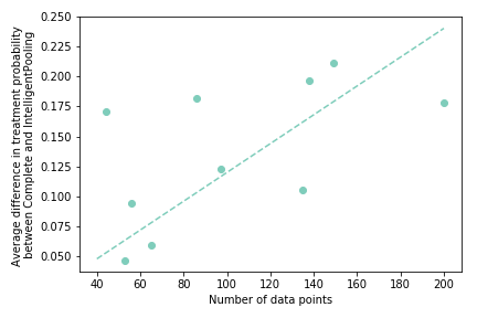
Figure 6: The difference in treatment probabilities between IntelligentPooling and Complete as a function of the amount of data from a user. Each dot is a different user.

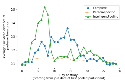
Figure 7: Mean squared distance between posterior and prior mean of the coefficients of $(A_{i,k}-\pi_{i,k})f(S_{i,k})$.

Speed of policy learning in Pilot We consider the speed at which IntelligentPooling diverges from the prior, relative to the speed of divergence for Person-Specific. Fig. 7 provides the Euclidean distance between the learned posterior and prior parameter vectors (averaged across the data from the 10 users at each time). From Fig. 7 we see that Person-Specific hardly varies over time in contrast to IntelligentPooling and Complete, which suggests that Person-Specific learns more slowly.

6 Conclusion

When data on individuals is limited a natural tension exists between personalizing (a choice which can introduce variance) and pooling (a choice which can introduce bias). In this work we have introduced a novel algorithm for personalized reinforcement learning, IntelligentPooling that presents a principled mechanism for balancing this tension. We demonstrate the practicality of our approach in the setting of mHealth. In simulation we achieve improvements of 26% over a state-of-the-art-method, while in a live clinical trial we show that our approach shows promise of personalization on even a limited number of users. We view adaptive pooling as a first step in addressing the trade-offs between personalization and pooling. The question of how to quantify the benefits/risks for individual users is an open direction for future work.

References

- Agrawal & Goyal (2012) Agrawal, Shipra and Goyal, Navin. Analysis of thompson sampling for the multi-armed bandit problem. In Conference on Learning Theory, 2012.
- Bogunovic et al. (2016) Bogunovic, Ilija, Scarlett, Jonathan, and Cevher, Volkan. Time-varying gaussian process bandit optimization. In Artificial Intelligence and Statistics, 2016.
- Bonilla et al. (2008) Bonilla, Edwin V, Chai, Kian M, and Williams, Christopher. Multi-task gaussian process prediction. In Advances in neural information processing systems, 2008.
- Boruvka et al. (2018) Boruvka, Audrey, Almirall, Daniel, Witkiewitz, Katie, and Murphy, Susan A. Assessing time-varying causal effect moderation in mobile health. Journal of the American Statistical Association, 113(523), 2018.
- Bouneffouf et al. (2012) Bouneffouf, Djallel, Bouzeghoub, Amel, and Gançarski, Alda Lopes. Hybrid--greedy for mobile context-aware recommender system. In Pacific-Asia Conference on Knowledge Discovery and Data Mining. Springer, 2012.
- Brochu et al. (2010) Brochu, Eric, Hoffman, Matthew W, and de Freitas, Nando. Portfolio allocation for bayesian optimization. arXiv preprint arXiv:1009.5419, 2010.
- Carlin & Louis (2010) Carlin, Bradley P and Louis, Thomas A. Bayes and empirical Bayes methods for data analysis. Chapman and Hall/CRC, 2010.
- Cesa-Bianchi et al. (2013) Cesa-Bianchi, Nicolo, Gentile, Claudio, and Zappella, Giovanni. A gang of bandits. In Advances in Neural Information Processing Systems, pp. 737–745, 2013.
- Chowdhury & Gopalan (2017) Chowdhury, Sayak Ray and Gopalan, Aditya. On kernelized multi-armed bandits. In Proceedings of the 34th International Conference on Machine Learning-Volume 70, 2017.
- Clarke et al. (2017) Clarke, Shanice, Jaimes, Luis G, and Labrador, Miguel A. mstress: A mobile recommender system for just-in-time interventions for stress. In 2017 14th IEEE Annual Consumer Communications & Networking Conference (CCNC), 2017.
- Consolvo et al. (2008) Consolvo, Sunny, McDonald, David W, Toscos, Tammy, Chen, Mike Y, Froehlich, Jon, Harrison, Beverly, Klasnja, Predrag, LaMarca, Anthony, LeGrand, Louis, Libby, Ryan, et al. Activity sensing in the wild: a field trial of ubifit garden. In Proceedings of the SIGCHI conference on human factors in computing systems, pp. 1797–1806, 2008.
- Desautels et al. (2014) Desautels, Thomas, Krause, Andreas, and Burdick, Joel W. Parallelizing exploration-exploitation tradeoffs in gaussian process bandit optimization. The Journal of Machine Learning Research, 15(1), 2014.
- Deshmukh et al. (2017) Deshmukh, Aniket Anand, Dogan, Urun, and Scott, Clay. Multi-task learning for contextual bandits. In Advances in Neural Information Processing Systems, 2017.
- Djolonga et al. (2013) Djolonga, Josip, Krause, Andreas, and Cevher, Volkan. High-dimensional gaussian process bandits. In Advances in Neural Information Processing Systems, 2013.
- Forman et al. (2018) Forman, Evan M, Kerrigan, Stephanie G, Butryn, Meghan L, Juarascio, Adrienne S, Manasse, Stephanie M, Ontañón, Santiago, Dallal, Diane H, Crochiere, Rebecca J, and Moskow, Danielle. Can the artificial intelligence technique of reinforcement learning use continuously-monitored digital data to optimize treatment for weight loss? Journal of behavioral medicine, 2018.
- Gardner et al. (2018) Gardner, Jacob, Pleiss, Geoff, Weinberger, Kilian Q, Bindel, David, and Wilson, Andrew G. Gpytorch: Blackbox matrix-matrix gaussian process inference with gpu acceleration. In Advances in Neural Information Processing Systems, 2018.
- Greenewald et al. (2017) Greenewald, Kristjan, Tewari, Ambuj, Murphy, Susan, and Klasnja, Predag. Action centered contextual bandits. In Advances in neural information processing systems, 2017.
- Hamine et al. (2015) Hamine, Saee, Gerth-Guyette, Emily, Faulx, Dunia, Green, Beverly B, and Ginsburg, Amy Sarah. Impact of mhealth chronic disease management on treatment adherence and patient outcomes: a systematic review. Journal of medical Internet research, 17(2):e52, 2015.
- Jaimes et al. (2016) Jaimes, Luis G, Llofriu, Martin, and Raij, Andrew. Preventer, a selection mechanism for just-in-time preventive interventions. IEEE Transactions on Affective Computing, 7(3), 2016.
- Kaewkannate & Kim (2016) Kaewkannate, Kanitthika and Kim, Soochan. A comparison of wearable fitness devices. BMC public health, 16(1), 2016.
- Krause & Ong (2011) Krause, Andreas and Ong, Cheng S. Contextual gaussian process bandit optimization. In Advances in Neural Information Processing Systems, 2011.
- Laird et al. (1982) Laird, Nan M, Ware, James H, et al. Random-effects models for longitudinal data. Biometrics, 38(4), 1982.
- Lawrence & Platt (2004) Lawrence, Neil D and Platt, John C. Learning to learn with the informative vector machine. In Proceedings of the twenty-first international conference on Machine learning, 2004.
- Li et al. (2010) Li, Lihong, Chu, Wei, Langford, John, and Schapire, Robert E. A contextual-bandit approach to personalized news article recommendation. In Proceedings of the 19th international conference on World wide web, 2010.
- Li & Kar (2015) Li, Shuai and Kar, Purushottam. Context-aware bandits. arXiv preprint arXiv:1510.03164, 2015.
- Liao et al. (2016) Liao, Peng, Klasnja, Predrag, Tewari, Ambuj, and Murphy, Susan A. Sample size calculations for micro-randomized trials in mhealth. Statistics in medicine, 35(12), 2016.
- Luo et al. (2018) Luo, Linkai, Yao, Yuan, Gao, Furong, and Zhao, Chunhui. Mixed-effects gaussian process modeling approach with application in injection molding processes. Journal of Process Control, 62, 2018.
- Nahum-Shani et al. (2017) Nahum-Shani, Inbal, Smith, Shawna N, Spring, Bonnie J, Collins, Linda M, Witkiewitz, Katie, Tewari, Ambuj, and Murphy, Susan A. Just-in-time adaptive interventions (jitais) in mobile health: key components and design principles for ongoing health behavior support. Annals of Behavioral Medicine, 52(6), 2017.
- Paredes et al. (2014) Paredes, Pablo, Gilad-Bachrach, Ran, Czerwinski, Mary, Roseway, Asta, Rowan, Kael, and Hernandez, Javier. Poptherapy: Coping with stress through pop-culture. In Proceedings of the 8th International Conference on Pervasive Computing Technologies for Healthcare. ICST (Institute for Computer Sciences, Social-Informatics and …, 2014.
- Rabbi et al. (2015) Rabbi, Mashfiqui, Aung, Min Hane, Zhang, Mi, and Choudhury, Tanzeem. Mybehavior: automatic personalized health feedback from user behaviors and preferences using smartphones. In Proceedings of the 2015 ACM International Joint Conference on Pervasive and Ubiquitous Computing. ACM, 2015.
- Rabbi et al. (2017) Rabbi, Mashfiqui, Philyaw-Kotov, Meredith, Lee, Jinseok, Mansour, Anthony, Dent, Laura, Wang, Xiaolei, Cunningham, Rebecca, Bonar, Erin, Nahum-Shani, Inbal, Klasnja, Predrag, et al. Sara: a mobile app to engage users in health data collection. In Proceedings of the 2017 ACM International Joint Conference on Pervasive and Ubiquitous Computing and Proceedings of the 2017 ACM International Symposium on Wearable Computers, pp. 781–789, 2017.
- Raudenbush & Bryk (2002) Raudenbush, Stephen W and Bryk, Anthony S. Hierarchical linear models: Applications and data analysis methods, volume 1. 2002.
- Shi et al. (2012) Shi, JQ, Wang, B, Will, EJ, and West, RM. Mixed-effects gaussian process functional regression models with application to dose–response curve prediction. Statistics in medicine, 31(26), 2012.
- Srinivas et al. (2009) Srinivas, Niranjan, Krause, Andreas, Kakade, Sham M, and Seeger, Matthias. Gaussian process optimization in the bandit setting: No regret and experimental design. arXiv preprint arXiv:0912.3995, 2009.
- Vaswani et al. (2017) Vaswani, Sharan, Schmidt, Mark, and Lakshmanan, Laks. Horde of bandits using gaussian markov random fields. In Artificial Intelligence and Statistics, 2017.
- Wang & Khardon (2012) Wang, Yuyang and Khardon, Roni. Nonparametric bayesian mixed-effect model: A sparse gaussian process approach. arXiv preprint arXiv:1211.6653, 2012.
- Wang et al. (2016) Wang, Zi, Zhou, Bolei, and Jegelka, Stefanie. Optimization as estimation with gaussian processes in bandit settings. In Artificial Intelligence and Statistics, 2016.
- Yom-Tov et al. (2017) Yom-Tov, Elad, Feraru, Guy, Kozdoba, Mark, Mannor, Shie, Tennenholtz, Moshe, and Hochberg, Irit. Encouraging physical activity in patients with diabetes: intervention using a reinforcement learning system. Journal of medical Internet research, 19(10), 2017.
- Zhou et al. (2018) Zhou, Mo, Mintz, Yonatan, Fukuoka, Yoshimi, Goldberg, Ken, Flowers, Elena, Kaminsky, Philip, Castillejo, Alejandro, and Aswani, Anil. Personalizing mobile fitness apps using reinforcement learning. In IUI Workshops, 2018.