The Whitham Equation with Surface Tension

Abstract.

The viability of the Whitham equation as a nonlocal model for capillary-gravity waves at the surface of an inviscid incompressible fluid is under study. A nonlocal Hamiltonian system of model equations is derived using the Hamiltonian structure of the free surface water wave problem and the Dirichlet-Neumann operator. The system features gravitational and capillary effects, and when restricted to one-way propagation, the system reduces to the capillary Whitham equation.

It is shown numerically that in various scaling regimes the Whitham equation gives a more accurate approximation of the free-surface problem for the Euler system than other models like the KdV, and Kawahara equation. In the case of relatively strong capillarity considered here, the KdV and Kawahara equations outperform the Whitham equation with surface tension only for very long waves with negative polarity.

1. Introduction

We consider the water-wave problem for a layer of an incompressible inviscid fluid bounded by a flat impenetrable bottom from below and by a free surface from above. The layer extends to infinity in the horizontal directions. It is a matter of common knowledge that the Euler equations with appropriate boundary conditions give a complete description of the liquid dynamics. However, in many cases the dynamics of the surface of solutions is of particular interest. To avoid heavy computations and concentrate attention only on the free surface, several models approximating evolution of the surface fluid displacement have been used. These model equations describe only the surface dynamics without providing complete solutions in the bulk of the fluid. The present work focuses on the derivation of a non-local water-wave model known as the Whitham equation that is fully dispersive in the linear approximation. In particular, we extend here the results of the work [27] to the case where surface tension is taken into account. The model equation under study is written as

$$\eta_{t}+W\eta_{x}+\frac{3}{2}\eta\eta_{x}=0,$$ (1.1)

where the convolution kernel of the operator $W\eta_{x}=w(-i\partial_{x})\eta_{x}=\big{(}{\mathcal{F}}^{-1}w\big{)}*\eta_{x}$ is given in terms of the Fourier transform by

$$w(\xi)=\sqrt{(1+\varkappa\xi^{2}){\textstyle{\frac{\tanh(\xi)}{\xi}}}}.$$ (1.2)

Here it is assumed that the variables are suitably normalized so that the gravitational acceleration, the undisturbed depth of the fluid and the density are all unity. The surface fluid tension is included here by means of the capillarity parameter $\varkappa$ which is the inverse of the Bond number. The convolution can be thought of as a Fourier multiplier operator, and (1.2) represents the Fourier symbol of the operator. It is also convenient from the analytical point of view to regard the Whitham operator $W=w(-i\partial_{x})$ as an integral with respect to the spectral measure of the self-adjoint operator $-i\partial_{x}$ in $L^{2}(\mathbb{R})$. Thus after linearization (1.1) can be considered as a Schrödinger equation with the self-adjoint operator $-i\partial_{x}w(-i\partial_{x})$. Indeed, introducing operator $D=-i\partial_{x}$ one may rewrite (1.1) as

$$i\eta_{t}=Dw(D)\eta+\frac{3}{4}D\eta^{2}.$$

From this point of view, for example, one may deduce straight away that for any real valued solution $\eta\in C^{1}(\mathbb{R},L^{2}(\mathbb{R}))$ of this equation the $L^{2}$-norm does not depend on time.

The Whitham equation was proposed by Whitham [34] as an alternative to the well known Korteweg-de Vries (KdV) equation

$$\eta_{t}+\eta_{x}+\frac{3}{2}\eta\eta_{x}-\frac{1}{2}\left(\varkappa-\frac{1}{3}\right)\eta_{xxx}=0.$$ (1.3)

Provided $\varkappa<1/3$ one may rescale $x$ and $t$ by $\sqrt{1-3\varkappa}$ and arrive at the equation

$$\eta_{t}+\eta_{x}+\frac{3}{2}\eta\eta_{x}+\frac{1}{6}\eta_{xxx}=0.$$

Thus it is apparent that small capillary effect do not add anything new to the KdV model. However, when $\varkappa$ is near $1/3$ one cannot expect that this model be applicable. To describe surface waves in such a situation, one may use instead the fifth-order-model equation

$$\eta_{t}+\eta_{x}+\frac{3}{2}\eta\eta_{x}-\frac{1}{2}\left(\varkappa-\frac{1}{3}\right)\eta_{xxx}+\frac{1}{360}(19-30\varkappa-45\varkappa^{2})\eta_{xxxxx}=0.$$ (1.4)

In our numerical experiments we use $\varkappa=1/3$, so that the equation reduces to what is known as the Kawahara equation [3, 6, 20], which has the following form:

$$\eta_{t}+\eta_{x}+\frac{3}{2}\eta\eta_{x}+\frac{1}{90}\eta_{xxxxx}=0.$$

The validity of the KdV and Kawahara equations can be described in the terms of the Stokes number $\mathcal{S}=\alpha\lambda^{2}$ where $\alpha=a/h_{0}$ and $\lambda/h_{0}$ represent a prominent amplitude and a characteristic wavelength of the wave field respectively. The KdV equation is known to be a good model for water waves if the amplitude of the waves is small and the wavelength is large when compared to the undisturbed depth, and if in addition, the two non-dimensional quantities $\alpha$ and $1/\lambda^{2}$ are of similar size which means $\mathcal{S}\sim 1$. With the same requirement and $\varkappa$ near $1/3$ the Kawahara equation gives better results for waves where capillarity is important. An alternative model where the air density above the free surface is taken into account was proposed in [33]. Another alternative model to the KdV equation (1.3) known as the BBM equation was put forward in [30] and studied in depth in [4]. The corresponding model with the capillarity $\varkappa$ has the form

$$\eta_{t}+\eta_{x}+\frac{3}{2}\eta\eta_{x}+\frac{1}{2}\left(\varkappa-\frac{1}{3}\right)\eta_{xxt}=0.$$ (1.5)

The linearized dispersion relation of this equation is not an exact match to the dispersion relation of the full water-wave problem, but it is much closer than the KdV equation in the case when $\varkappa<1/3$, and it might also be expected that this equation may be able to model shorter waves more successfully than the KdV equation. However, the domain of its applicability is $\mathcal{S}\sim 1$, that coincides with the corresponding restrictions of the KdV model [4]. One may also notice that (1.5) can also be scaled to the equation without capillarity in the same way as (1.3) providing capillarity $\varkappa$ is small.

Both KdV and Kawahara equations are generally believed to approximate very long waves quite well, but one notorious problem with these equations is that they do not model accurately the dynamics of shorter waves. Recognizing this shortcoming of the KdV equation, Whitham proposed to use the same nonlinearity as the KdV equation, but coupled with a linear term which mimics the linear dispersion relation of the full water-wave problem. Thus, at least in theory, the Whitham equation can be expected to yield a description of the dynamics of shorter waves which is closer to the governing Euler equations. The Whitham equation (1.1) has been studied from a number of vantage points during recent years. In particular, the existence of traveling and solitary waves has been studied [1, 13, 14, 15]. Well posedness of a similar equation was investigated in [22], and similar full dispersion equations were also studied in [23]. Moreover, it has been shown in [18, 19, 32] that periodic solutions of equation (1.1) feature modulational instability for short enough waves in a similar way as small-amplitude periodic wave solutions of the water-wave problem. The performance of the Whitham equation in the description of surface water waves has been investigated in [5] in the steady case without surface tension. However, it appears that no study of the performance of the Whitham equation in the presence of capillarity has been done.

In the present note, we give an asymptotic derivation of the Whitham equation as a model for surface water waves, giving close consideration to the influence of the surface tension. The derivation proceeds by examining the Hamiltonian formulation of the water-wave problem due to Zhakarov, Craig and Sulem [36, 10]. This approach is similar to the method of [8]. However, our consideration is not constrained heavily by any particular scalar regime. Firstly, a corresponding Whitham system is derived, and then the Whitham equation is found by restricting the system to one-way propagation. Secondly, we derive different models from the Whitham equation and point out the corresponding domains of their applicability.

Finally, a numerical comparison of modeling properties of the KdV, Kawahara and Whitham equations is given with respect to the Euler system.

2. Euler system and its Hamiltonian

The surface water-wave problem is generally described by the Euler equations with no-flow conditions at the bottom, and kinematic and dynamic boundary conditions at the free surface. Assuming weak transverse effects, the unknowns are the surface elevation $\eta(x,t)$, the horizontal and vertical fluid velocities $u_{1}(x,z,t)$ and $u_{2}(x,z,t)$, respectively, and the pressure $P(x,z,t)$. If the assumption of irrotational flow is made, then a velocity potential $\phi(x,z,t)$ can be used. Taking the undisturbed depth $h_{0}=1$ as a unit of distance, and the parameter $\sqrt{h_{0}/g}=1$ as a unit of time, the problem may be posed on a domain $\left\{(x,z)\in\mathbb{R}^{2}|-1<z<\eta(x,t)\right\}$ which extends to infinity in the positive and negative $x$-direction. Due to the incompressibility of the fluid, the potential then satisfies the Laplace’s equation in this domain. The fact that the fluid cannot penetrate the bottom is expressed by a homogeneous Neumann boundary condition at the flat bottom. Thus we have

$$\phi_{xx}+\phi_{zz}=0 -1<z<\eta(x,t)$$ in

$$\phi_{z}=0 z=-1.$$ on

The pressure is eliminated with help of the Bernoulli equation, and the free-surface boundary conditions are formulated in terms of the potential $\varphi$ and the surface displacement $\eta$ by

$$\left.\begin{array}[]{rc}\eta_{t}+\phi_{x}\eta_{x}-\phi_{z}&=0,\\ \phi_{t}+\frac{1}{2}\big{(}\phi^{2}_{x}+\phi^{2}_{z}\big{)}+\eta-\varkappa\eta_{xx}\big{(}1+\eta_{x}^{2}\big{)}^{-3/2}&=0,\end{array}\right\}\mbox{on}\ z=\eta(x,t).$$

The first equation represents the definition of the fluid velocity with respect to the Euler coordinates. The second one is the Bernoulli equation with the capillary term.

The total energy of the system is given by the sum of the kinetic energy, the potential energy and the surface tension energy, and normalized in such a way that the total energy is zero when no wave motion is present at the surface. Accordingly the Hamiltonian function for this problem is

$$H=\int_{\mathbb{R}}\int_{0}^{\eta}z\,dzdx+\int_{\mathbb{R}}\int_{-1}^{\eta}{\textstyle{\frac{1}{2}}}|\nabla\phi|^{2}\,dzdx+\varkappa\int_{\mathbb{R}}{\textstyle{\frac{\eta_{x}^{2}}{1+\sqrt{1+\eta_{x}^{2}}}}}dx.$$

Defining the trace of the potential at the free surface as $\Phi(x,t)=\phi(x,\eta(x,t),t)$, one may integrate in $z$ in the first integral and use the divergence theorem on the second integral in order to arrive at the formulation

$$H=\int_{\mathbb{R}}\Big{[}{\textstyle{\frac{1}{2}}}\eta^{2}+{\textstyle{\frac{1}{2}}}\Phi G(\eta)\Phi+\varkappa{\textstyle{\frac{\eta_{x}^{2}}{1+\sqrt{1+\eta_{x}^{2}}}}}\Big{]}\,dx.$$ (2.1)

This is the Hamiltonian of the water wave problem with surface tension as for instance found in [2], and written in terms of the Dirichlet-Neumann operator $G(\eta)$. As shown in [28], the Dirichlet-Neumann operator is analytic in a certain sense, and can be expanded as a power series as

$$G(\eta)\Phi=\sum_{j=0}^{\infty}G_{j}(\eta)\Phi.$$

In order to proceed, we need to understand the first few terms in this series. As shown in [10] and [8], the first two terms in this series can be written with the help of the operator $D=-i\partial_{x}$ as

$$G_{0}(\eta)=D\tanh(D),\qquad G_{1}(\eta)=D\eta D-D\tanh(D)\eta D\tanh(D).$$

Note that it can be shown that the terms $G_{j}(\eta)$ for $j\geq 2$ are of quadratic or higher-order in $\eta$, and will therefore not be needed in the following analysis.

It will be convenient for the present purpose to formulate the Hamiltonian in terms of the dependent variable $u=\Phi_{x}$. This new variable is proportional to the velocity of the fluid tangential to the surface. More precisely $u=\varphi_{x}+\eta_{x}\varphi_{z}=\varphi_{\tau}\sqrt{1+\eta_{x}^{2}}$ where $\varphi_{\tau}$ is exactly the tangential velocity component to the surface. To this end, we define the operator $\mathcal{K}$ by

$$G(\eta)=D\mathcal{K}(\eta)D.$$

As was the case with $G(\eta)$, the operator $\mathcal{K}(\eta)$ can also be expanded in a Taylor series with respect to powers of $\eta$ and $\eta_{x}$ as

$$\mathcal{K}(\eta)=\sum_{j=0}^{\infty}\mathcal{K}_{j}(\eta),\qquad\mathcal{K}_{j}(\eta)=D^{-1}G_{j}(\eta)D^{-1}.$$

In particular, note that $\mathcal{K}_{0}=\tanh{D}/D$ and $\mathcal{K}_{1}=\eta-\tanh{D}(\eta\tanh{D})$. After integrating by parts the Hamiltonian can be expressed as

$$H=\int_{\mathbb{R}}\Big{[}{\textstyle{\frac{1}{2}}}\eta^{2}+{\textstyle{\frac{1}{2}}}u\mathcal{K}(\eta)u+\varkappa{\textstyle{\frac{\eta_{x}^{2}}{1+\sqrt{1+\eta_{x}^{2}}}}}\Big{]}\,dx.$$ (2.2)

The following analysis has the formal character of long-wave approximation. Consider a wave-field having a characteristic non-dimensional wavelength $\lambda$ and a characteristic non-dimensional amplitude $\alpha$. We also introduce the small parameter $\mu=\frac{1}{\lambda}$. To obtain different approximations of the discussed problem the amplitude $\alpha$ is considered as a function of wave-number $\mu$. Its behavior at small wave-numbers defines different scaling regimes. The long-wave approximation means the scale $\eta=O(\alpha)$, $u=O(\alpha)$ and $D=-i\partial_{x}=O(\mu)$ where $\alpha=\alpha(\mu)$ depends on the small parameter $\mu$. Now the Hamiltonian (2.2) may be simplified as follows

$$H=H_{g}+H_{c}+O(\mu^{2}\alpha^{4})$$ (2.3)

with the gravity term

$$H_{g}=\frac{1}{2}\int_{\mathbb{R}}\Big{[}\eta^{2}+u{\textstyle{\frac{\tanh D}{D}}}u+\eta u^{2}-u\tanh{D}(\eta\tanh{D}u)\Big{]}dx$$ (2.4)

and the capillary part

$$H_{c}=\varkappa\int_{\mathbb{R}}{\textstyle{\frac{\eta_{x}^{2}dx}{1+\sqrt{1+\eta_{x}^{2}}}}}=\frac{\varkappa}{2}\int_{\mathbb{R}}\eta_{x}^{2}dx+O(\mu^{4}\alpha^{4}).$$ (2.5)

Before we continue with derivation of the Whitham equation we prove the following lemma about integration by parts, which is certainly well-known and we add it here only for completeness.

Lemma 2.1.

Let $f,g$ be real-valued square integrable functions on real axis $\mathbb{R}$. Regard $D=-i\partial_{x}$ as self-adjoint on $L^{2}(\mathbb{R},\mathbb{C})$ and a real-valued function $\varphi$ that is measurable and almost everywhere finite with respect to Lebesgue measure. If $f,g$ lie in the domain of the operator $\varphi(D)$ then

$$\int f\varphi(D)g=\int g\varphi(-D)f$$

Proof.

It is given two proofs below. The first one is to regard $\varphi(D)=(\mathcal{F}^{-1}\varphi)*$ as the operator of convolution in the sense of distribution theory

$$\int f\varphi(D)g=\int f(\xi)(\mathcal{F}^{-1}\varphi)(\xi-x)g(x)dxd\xi=\\ =\int f(\xi)(\mathcal{F}^{-1}\varphi\circ(-id))(x-\xi)g(x)dxd\xi=\int g\varphi(-D)f.$$

The second proof is to represent $\varphi(D)=\int\varphi dE$ as the integral with respect to spectral measure $E$ of the operator $D$. The corresponding projector of the interval $(\alpha,\beta)$ is the convolution with the function $e_{(\alpha,\beta)}(x)=\frac{1}{2\pi ix}(e^{i\beta x}-e^{i\alpha x})$. So the replacement of $f$ and $g$ changes the corresponding spectral complex measure of intervals as follows

$$\mu_{f,g}(\alpha,\beta)=(E(\alpha,\beta)f,g)=\int e_{(\alpha,\beta)}(x-y)f(y)g(x)dxdy=\\ =\int e_{(-\beta,-\alpha)}(y-x)f(y)g(x)dxdy=\mu_{g,f}(-\beta,-\alpha)$$

which implies the statement of the lemma

$$\int f\varphi(D)g=\int\varphi(x)d\mu_{g,f}(x)=\int\varphi(-x)d\mu_{f,g}(x)=\int g\varphi(-D)f.$$

∎

3. Derivation of the Whitham type evolution system

The water-wave problem can be rewritten as a Hamiltonian system using the variational derivatives of $H$. Making reference to [8, 9] note that the pair $(\eta,\Phi)$ represents the canonical variables for the Hamiltonian function (2.1). However, it is more common to write the equations of motion in the fluid dynamics of free surface in terms of $\eta$ and $u=\Phi_{x}$. The transformation $(\eta,\Phi)\mapsto(\eta,u)$ is associated with the Jacobian

$$\frac{\partial(\eta,u)}{\partial(\eta,\Phi)}=\begin{pmatrix}1&0\\ 0&\partial_{x}\end{pmatrix}.$$

Thus in terms of $\eta$ and $u$ the Hamiltonian equations have the form

$$\eta_{t}=-\partial_{x}\frac{\delta H}{\delta u},\qquad u_{t}=-\partial_{x}\frac{\delta H}{\delta\eta}$$ (3.1)

that is not canonical since the associated structure map $J_{\eta,u}$ is symmetric:

$$J_{\eta,u}=\left(\frac{\partial(\eta,u)}{\partial(\eta,\Phi)}\right)\begin{pmatrix}0&1\\ -1&0\end{pmatrix}\left(\frac{\partial(\eta,u)}{\partial(\eta,\Phi)}\right)^{*}=\begin{pmatrix}0&-\partial_{x}\\ -\partial_{x}&0\end{pmatrix}.$$

We now derive a system of equations which is similar to the Whitham equation (1.1), but admits bi-directional wave propagation. The variational derivative ${\delta H_{g}}/{\delta u}$ is defined by means of any real-valued square integrable function $h$ as follows

$$\int_{\mathbb{R}}\frac{\delta H_{g}}{\delta u}(x)h(x)dx=d_{u}H_{g}h=\left.\frac{d}{d\tau}\right|_{\tau=0}H_{g}(u+\tau h,\eta)=\int_{\mathbb{R}}u\eta hdx+\\ +\frac{1}{2}\int_{\mathbb{R}}\Big{[}h{\textstyle{\frac{\tanh D}{D}}}u+u{\textstyle{\frac{\tanh D}{D}}}h-h\tanh{D}(\eta\tanh{D}u)-u\tanh{D}(\eta\tanh{D}h)\Big{]}dx.$$

Making use of integration by parts described in Lemma 2.1 one obtains

$$\frac{\delta H_{g}}{\delta u}=\frac{\tanh D}{D}u+\eta u-\tanh{D}(\eta\tanh{D}u)=\frac{\tanh D}{D}u+\eta u+O(\mu^{2}\alpha^{2})$$

and in the same way

$$\frac{\delta H_{g}}{\delta\eta}=\eta+\frac{1}{2}u^{2}+\frac{1}{2}(\tanh{D}u)^{2}=\eta+\frac{1}{2}u^{2}+O(\mu^{2}\alpha^{2}).$$

These variational derivatives were also obtained by Moldabayev and Kalisch [27]. The capillary part $H_{c}$ defined by (2.5) gives the pressure $P$ on the surface

$$\frac{\delta H_{c}}{\delta\eta}=-\varkappa\frac{\eta_{xx}}{(1+\eta_{x}^{2})^{\frac{3}{2}}}=-\varkappa\eta_{xx}+O(\mu^{4}\alpha^{3}).$$

At last the Hamilton system (3.1) is simplified to the Whitham system

$$\eta_{t} =-\frac{\tanh D}{D}u_{x}-(\eta u)_{x}+\tanh{D}(\eta\tanh{D}u)_{x}+O(\mu^{3}\alpha^{3}),$$ (3.2)

$$u_{t} =-\eta_{x}-uu_{x}-(\tanh{D}u)\tanh{D}u_{x}+\varkappa\eta_{xxx}+O(\mu^{3}\alpha^{3})$$ (3.3)

which is in line with the system obtained in [27]

$$\eta_{t} =-\frac{\tanh D}{D}u_{x}-(\eta u)_{x}+O(\mu^{3}\alpha^{2}),$$

$$u_{t} =-\eta_{x}-uu_{x}+\varkappa\eta_{xxx}+O(\mu^{3}\alpha^{2}).$$

4. Derivation of Whitham type evolution equations

It turns out that the Whitham system (3.2), (3.3) might be rewritten as a system of two independent equations by further simplification. More precisely, they will be independent with respect to the linear approximation of that system. For this purpose we need to separate solutions corresponding to waves moving in other directions. In order to derive the Whitham equation for uni-directional wave propagation, it is important to understand how one-way propagation works in the Whitham system (3.2), (3.3). Regard the linearisation of this system

$$\eta_{t}+\frac{\tanh D}{D}u_{x} =0,$$ (4.1)

$$u_{t}+(1+\varkappa D^{2})\eta_{x} =0.$$ (4.2)

Regarding solutions of this linear system in the wave form

$$\eta(x,t)=Ae^{i\xi x-i\omega t},\qquad u(x,t)=Be^{i\xi x-i\omega t}$$

gives rise to the matrix equation

$$\begin{pmatrix}-\omega&\tanh\xi\cr\xi+\varkappa\xi^{3}&-\omega\end{pmatrix}\begin{pmatrix}A\cr B\end{pmatrix}=\begin{pmatrix}0\cr 0\end{pmatrix}.$$

This equation has a non-trivial solution, provided its determinant equals zero, so that $\omega^{2}-(\xi+\varkappa\xi^{3})\tanh\xi=0$. Defining the phase speed as $c=\omega(\xi)/\xi$ one obtains the dispersion relation

$$c^{2}(\xi)=(1+\varkappa\xi^{2})\frac{\tanh\xi}{\xi}$$

which coincides, up to the sign of $c$, with Whitham dispersion relation (1.2). Obviously, the choice $c>0$ corresponds to right-going wave solutions of the linear system (4.1), (4.2). And the phase speed $c<0$ gives left-going waves. To split up these two kinds of waves we regard the following transformation of variables

$$r=\frac{1}{2}(\eta+Ku),\qquad s=\frac{1}{2}(\eta-Ku).$$ (4.3)

It is supposed that $K$ is an invertible operator, namely an invertible function of the differential operator $D$. The inverse transformation has the form

$$\eta=r+s,\qquad u=K^{-1}(r-s).$$ (4.4)

The question arises whether it is possible to choose such operator $K$ that $r$ and $s$ correspond to right- and left-going waves, respectively. After applying the transformation (4.4) to the linear system (4.1), (4.2) one arrives to the system

$$r_{t}+\partial_{x}\big{(}A(D,K)r+B(D,K)s\big{)} =0,$$

$$s_{t}-\partial_{x}\big{(}A(D,K)s+B(D,K)r\big{)} =0$$

where operators $A$ and $B$ depend on $D$ and $K$ as follows

$$A=\frac{1}{2}\left((1+\varkappa D^{2})K+\frac{\tanh D}{D}K^{-1}\right),\qquad B=\frac{1}{2}\left((1+\varkappa D^{2})K-\frac{\tanh D}{D}K^{-1}\right).$$

So to achieve independence of the obtained two equations we need to choose the transformation $K$ in the way $B(D,K)=0$, so that

$$K=\sqrt{\frac{1}{1+\varkappa D^{2}}\cdot\frac{\tanh D}{D}}$$ (4.5)

which leads to the two independent Whitham equations

$$r_{t}+\partial_{x}Wr =0,$$ (4.6)

$$s_{t}-\partial_{x}Ws =0$$ (4.7)

where the Whitham operator $W=w(D)=A(D,K)$ was introduced at the beginning of the paper by (1.2). If we again regard the wave solutions $r(x,t)=\exp({i\xi x-i\omega_{r}t})$ and $s(x,t)=\exp({i\xi x-i\omega_{s}t})$ then we conclude that the first equation (4.6) describes waves moving to the right with the phase velocity $c_{r}=\omega_{r}/\xi=w(\xi)$ and the second equation (4.7) corresponds to the left-going waves with $c_{s}=\omega_{s}/\xi=-w(\xi)$.

Now we regard the Hamiltonian (2.2) as a functional of $r$ and $s$ with the same long-wave approximation as before (2.3) where obviously $r=O(\alpha)$ and $s=O(\alpha)$. The unperturbed Hamiltonian part (2.4) is

$$H_{g}=\frac{1}{2}\int_{\mathbb{R}}\Big{[}(r+s)^{2}+\big{(}K^{-1}(r-s)\big{)}{\textstyle{\frac{\tanh D}{D}}}K^{-1}(r-s)+(r+s)\big{(}K^{-1}(r-s)\big{)}^{2}-\\ \big{(}K^{-1}(r-s)\big{)}\tanh{D}\big{(}(r+s)\tanh{D}K^{-1}(r-s)\big{)}\Big{]}dx$$ (4.8)

and the surface tension adding (2.5) is

$$H_{c}=\frac{\varkappa}{2}\int_{\mathbb{R}}(r+s)_{x}^{2}dx+O(\mu^{4}\alpha^{4}).$$ (4.9)

According to the transformation theory detailed in [9], due to the changing of variables (4.3) or (4.4), the structure map changes to

$$J_{r,s}=\left(\frac{\partial(r,s)}{\partial(\eta,u)}\right)J_{\eta,u}\left(\frac{\partial(r,s)}{\partial(\eta,u)}\right)^{*}=\begin{pmatrix}-\frac{1}{2}\partial_{x}K&0\\ 0&\frac{1}{2}\partial_{x}K\end{pmatrix}.$$

The corresponding Hamiltonian system has the form

$$r_{t}+\partial_{x}\left(\frac{K}{2}\frac{\delta H}{\delta r}\right)=0,\quad\quad s_{t}-\partial_{x}\left(\frac{K}{2}\frac{\delta H}{\delta s}\right)=0.$$ (4.10)

These equations are equivalent to (3.1). However, solutions $r(x,t)$ and $s(x,t)$ are the displacements going right and left, respectively, when a solution $u(x,t)$, representing the tangential velocity component up to the curvature multiplier, might not be imagined so easy. As above we calculate the Gâteaux derivative of $H_{g}$ given by (4.8) with respect to $r$ at a real-valued square integrable function

$$\int_{\mathbb{R}}\frac{\delta H_{g}}{\delta r}(x)h(x)dx=d_{r}H_{g}h=\left.\frac{d}{d\tau}\right|_{\tau=0}H_{g}(r+\tau h,s)=\int(r+s)h+\\ +\frac{1}{2}\int\big{(}K^{-1}h\big{)}\frac{\tanh D}{D}K^{-1}(r-s)+\frac{1}{2}\int\big{(}K^{-1}(r-s)\big{)}\frac{\tanh D}{D}K^{-1}h+\\ +\frac{1}{2}\int h\big{(}K^{-1}(r-s)\big{)}^{2}+\int(r+s)\big{(}K^{-1}(r-s)\big{)}K^{-1}h-\\ -\frac{1}{2}\int\big{(}K^{-1}h\big{)}\tanh{D}\big{(}(r+s)\tanh{D}K^{-1}(r-s)\big{)}-\\ -\frac{1}{2}\int\big{(}K^{-1}(r-s)\big{)}\tanh{D}\big{(}h\tanh{D}K^{-1}(r-s)\big{)}-\\ -\frac{1}{2}\int\big{(}K^{-1}(r-s)\big{)}\tanh{D}\big{(}(r+s)\tanh{D}K^{-1}h\big{)}.$$

Integrating by parts as in Lemma 2.1 and taking into account that functions $\tanh D$ is odd while $K$ is even (4.5) with respect to $D$ one can obtain ${\delta H_{g}}/{\delta r}$, and in the similar way ${\delta H_{c}}/{\delta r}$, ${\delta H_{g}}/{\delta s}$, ${\delta H_{c}}/{\delta s}$. Thus as a result

$$\frac{K}{2}\frac{\delta H}{\delta r}=Wr+\frac{1}{4}K\big{(}K^{-1}(r-s)\big{)}^{2}+\frac{1}{2}(r+s)K^{-1}(r-s)+\\ +\frac{1}{4}K\big{(}\tanh DK^{-1}(r-s)\big{)}^{2}-\frac{1}{2}\tanh D\big{(}(r+s)\tanh DK^{-1}(r-s)\big{)}+O(\mu^{2}\alpha^{3})$$ (4.11)

and

$$\frac{K}{2}\frac{\delta H}{\delta s}=Ws+\frac{1}{4}K\big{(}K^{-1}(r-s)\big{)}^{2}-\frac{1}{2}(r+s)K^{-1}(r-s)+\\ +\frac{1}{4}K\big{(}\tanh DK^{-1}(r-s)\big{)}^{2}+\frac{1}{2}\tanh D\big{(}(r+s)\tanh DK^{-1}(r-s)\big{)}+O(\mu^{2}\alpha^{3})$$ (4.12)

together with (4.10) are the Whitham system describing the displacement $\eta(x,t)$ in terms of waves going right and left. This system is entirely equivalent to (3.2), (3.3) and at the same time gives rise to solutions with more clear physical meaning. Another useful property of this system is that it can be enough to regard only one equation if we are allowed to neglect the waves going to a particular direction. More precisely, regarding only right-going waves leads to

$$\frac{K}{2}\frac{\delta H}{\delta r}=Wr+\frac{1}{4}K\big{(}K^{-1}r\big{)}^{2}+\frac{1}{2}rK^{-1}r+\\ +\frac{1}{4}K\big{(}\tanh DK^{-1}r\big{)}^{2}-\frac{1}{2}\tanh D\big{(}r\tanh DK^{-1}r\big{)}+O(\alpha|s|)+O(\mu^{2}\alpha^{3})$$ (4.13)

and only left-going waves gives

$$\frac{K}{2}\frac{\delta H}{\delta s}=Ws+\frac{1}{4}K\big{(}K^{-1}s\big{)}^{2}+\frac{1}{2}sK^{-1}s+\\ +\frac{1}{4}K\big{(}\tanh DK^{-1}s\big{)}^{2}-\frac{1}{2}\tanh D\big{(}s\tanh DK^{-1}s\big{)}+O(\alpha|r|)+O(\mu^{2}\alpha^{3}).$$ (4.14)

As one can see these expressions are identical up to discarded parts. Equality (4.13) together with the first equation of (4.10) corresponds to the Whitham equation describing right-going surface waves. Equality (4.14) together with the second equation of (4.10) corresponds to the Whitham equation describing left-going surface waves. Further simplifications can be made by studying concrete regimes $\alpha(\mu)$. As a matter of fact, examples of behavior $\alpha(\mu)$ at small $\mu$ that we regard below need less accurate asymptotic. So that operators $K$ and $\tanh D$ can still be simplified by taking into account $D=O(\mu)$ in Equality (4.13) as follows

$$\frac{K}{2}\frac{\delta H}{\delta r}=Wr+\frac{3}{4}r^{2}+\frac{1}{4}\left(\varkappa-\frac{5}{3}\right)rD^{2}r-\frac{1}{4}\left(\varkappa+\frac{4}{3}\right)(Dr)^{2}+\\ +O(\mu^{4}\alpha^{2})+O(\alpha|s|)+O(\mu^{2}\alpha^{3}).$$ (4.15)

It is in line with [27] for liquids without surface tension $\varkappa=0$. There is the same expression for the other variational derivative with replacement $r$ by $s$.

4.1. Linear approximation.

Let $r$ and $s$ be of the same order and $\alpha=o(1)$ as $\mu\to 0$. Then (4.13), (4.14) are simplified to

$$\frac{K}{2}\frac{\delta H}{\delta r}=Wr(1+o(1)),\qquad\frac{K}{2}\frac{\delta H}{\delta s}=Ws(1+o(1))$$

that together with (4.10) represent two independent linear equations. We again arrived to (4.6), (4.7). This is the case when we do not have enough information about order relation between right- and left-going waves.

4.2. The shallow-water scaling regime.

Let $\alpha=O(1)$ as $\mu\to 0$. Assume also that left-going waves can be discarded $s=o(1)$. In this case operators $W$ can also be simplified by taking into account $D=O(\mu)$. Expression (4.15) becomes

$$\frac{K}{2}\frac{\delta H}{\delta r}=r+\frac{3}{4}r^{2}+o(1)$$

which leads to the shallow-water equation

$$r_{t}+r_{x}+\frac{3}{2}rr_{x}=o(\mu).$$

4.3. The Boussinesq scaling regime.

Let $\alpha=O(\mu^{2})$ and $s=o(\mu^{2})$ as $\mu\to 0$. Expression (4.15) becomes

$$\frac{K}{2}\frac{\delta H}{\delta r}=Wr+\frac{3}{4}r^{2}+o(\mu^{4})$$

that can be simplified further by two different ways

$$W=1+\frac{1}{2}\left(\varkappa-\frac{1}{3}\right)D^{2}+O(\mu^{4})=\left(1-\frac{1}{2}\left(\varkappa-\frac{1}{3}\right)D^{2}\right)^{-1}+O(\mu^{4}).$$

The first equality leads to the KdV equation

$$r_{t}+r_{x}-\frac{1}{2}\left(\varkappa-\frac{1}{3}\right)r_{xxx}+\frac{3}{2}rr_{x}=o(\mu^{5}).$$

The second equality gives rise to the BBM equation

$$r_{t}+r_{x}+\frac{1}{2}\left(\varkappa-\frac{1}{3}\right)r_{xxt}+\frac{3}{2}rr_{x}=o(\mu^{5}).$$

4.4. The Padé (2,2) approximation.

Suppose $\alpha=O(\mu^{4})$ and $s=o(\mu^{4})$ as $\mu\to 0$. Expression (4.15) becomes

$$\frac{K}{2}\frac{\delta H}{\delta r}=Wr+\frac{3}{4}r^{2}+o(\mu^{8})$$

that can be simplified further provided $\varkappa\neq 1/3$ by the way

$$W=\frac{1+aD^{2}}{1+bD^{2}}+O(\mu^{6})$$

where constants $a$ and $b$ depend on $\varkappa$ as follows

$$a(\varkappa)=\frac{3+10\varkappa-45\varkappa^{2}}{20(1-3\varkappa)},$$

$$b(\varkappa)=\frac{19-30\varkappa-45\varkappa^{2}}{60(1-3\varkappa)}.$$

The corresponding equation

$$r_{t}+r_{x}-a(\varkappa)r_{xxx}-b(\varkappa)r_{xxt}+\frac{3}{2}rr_{x}=o(\mu^{9}).$$

As one can see the order of this differential equation is the same as the order of KdV or BBM, meanwhile the Padé approximation is more accurate. In the case $\varkappa=1/3$ one has to use the usual Taylor approximation

$$W=1+\frac{1}{2}\left(\varkappa-\frac{1}{3}\right)D^{2}+\frac{1}{360}(19-30\varkappa-45\varkappa^{2})D^{4}+O(\mu^{6})$$

which gives rise to the equation of fifth order

$$r_{t}+r_{x}-\frac{1}{2}\left(\varkappa-\frac{1}{3}\right)r_{xxx}+\frac{1}{360}(19-30\varkappa-45\varkappa^{2})r_{xxxxx}+\frac{3}{2}rr_{x}=o(\mu^{9})$$

that is the Kawahara equation (1.4).

4.5. The Whitham scaling regime.

If we now assume $\alpha=O(\mu^{N})$ for any positive integer $N$ and $s=o(\alpha)$ as $\mu\to 0$, then we arrive to an example when the Whitham operator $W$ cannot be approximated using a simple differential operator instead. The simplest equation in this case is the Whitham equation

$$r_{t}+Wr_{x}+\frac{3}{2}rr_{x}=o(\mu\alpha^{2}).$$

An example of the function $\alpha(\mu)$ when the Whitham equation works better than its approximations was given in [27]. At the same time that function $\alpha(\mu)$ may be similar to the Boussinesq scale at some wave-numbers $\mu$ as was pointed out in [27].

5. Numerical results

The purpose of this section is to compare the performance of the Whitham equation as a model for surface water waves to both the KdV equation (1.3) and to the Kawahara equation (1.4). In other words, all these approximate models are compared to the Euler system which is considered as giving the closest description of an actual surface wave profile. For this purpose initial data are imposed, the Whitham, KdV and Kawahara equations are solved with periodic boundary conditions, and the solutions are compared to the numerical solutions of the full Euler equations with free-surface boundary conditions. This matching is made in various scaling regimes from small Stokes numbers to $\mathcal{S}\sim 1$, to large Stokes numbers.

Experiment	Stokes number $\mathcal{S}$	Amplitude $\alpha$	Wavelength $\lambda$
A	1	0.1	$\sqrt{10}$
B	1	0.2	$\sqrt{5}$
C	10	0.1	10
D	10	0.2	$\sqrt{50}$
E	0.1	0.1	$1$
F	0.1	0.2	$\sqrt{1/2}$

Table 1. Summary of the Stokes number, nondimensional wavelength, nondimensional amplitude of the initial data used in the numerical experiments.

The numerical treatment of the three model equations is a standard spectral scheme, such as used in [16] and [15] for example. For the time stepping, an efficient fourth-order implicit method developed in [12] is used. The numerical discretization of the free-surface problem for the Euler equations is based on a conformal mapping of the fluid domain into a rectangle. In the case of transient dynamics, this method has roots in the work of Ovsyannikov [29], and was later used in [11] and [24]. In the case of periodic boundary conditions, a Fourier-spectral collocation method can be used for the computations, and the particular method used for the numerical experiments reported here is detailed in [26].

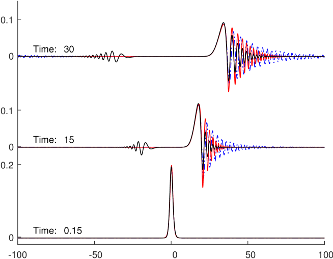
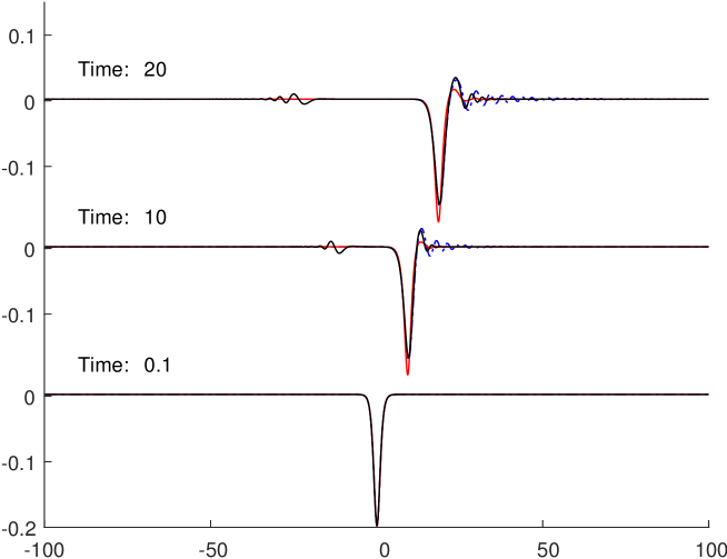
Figure 1. Wave profiles at three different times: – the Euler (black line), – Whitham (red line) and – KdV (blue line) with amplitude $\alpha=0.2$, wavelength $\lambda=\sqrt{5}$ and capillarity parameter $\varkappa=1/2$.

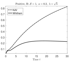
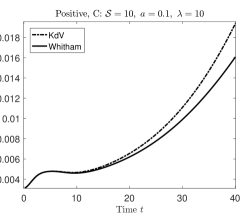
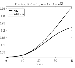
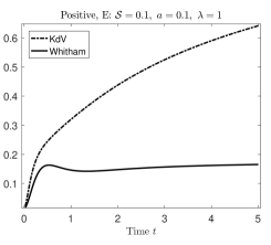
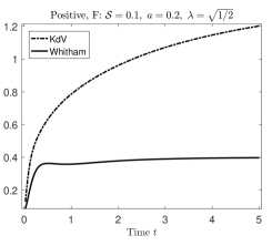
Figure 2. $L^{2}$ errors in approximation of solutions to the full Euler equations by different model equations with the positive initial wave $\eta_{0}(x)$ and the surface tension $\varkappa=\frac{1}{2}$.

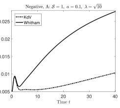
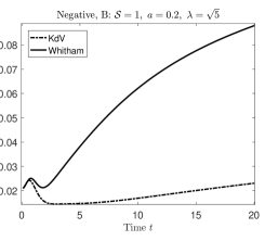
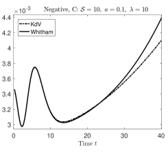
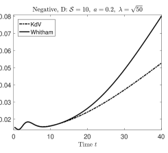
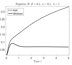
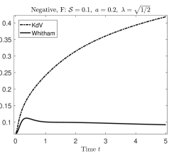
Figure 3. $L^{2}$ errors in approximation of solutions to the full Euler equations by different model equations with the negative initial wave $\eta_{0}(x)$ and the surface tension $\varkappa=\frac{1}{2}$.

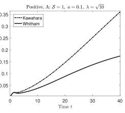
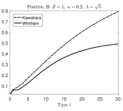
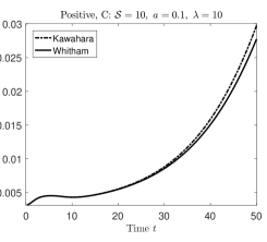
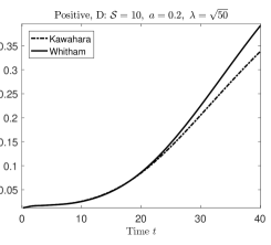
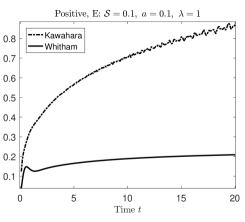
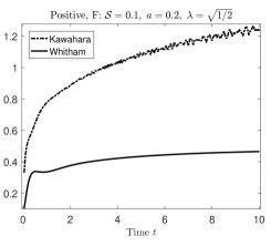
Figure 4. $L^{2}$ errors in approximation of solutions to the full Euler equations by different model equations with the positive initial wave $\eta_{0}(x)$ and the surface tension $\varkappa=\frac{1}{3}$.

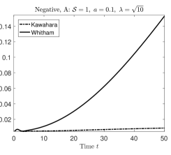
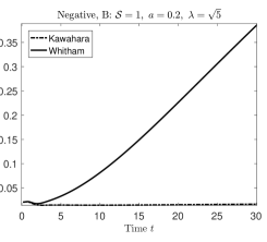
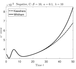
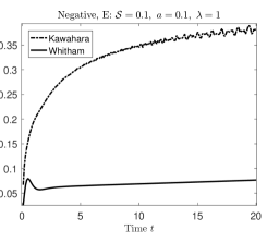
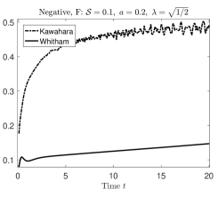
Figure 5. $L^{2}$ errors in approximation of solutions to the full Euler equations by different model equations with the negative initial wave $\eta_{0}(x)$ and the surface tension $\varkappa=\frac{1}{3}$.

Initial conditions for the Euler equations are chosen in such a way that the solutions are expected to be right moving. This can be achieved by imposing an initial surface disturbance $\eta_{0}$ together with the initial trace of the potential $\Phi(x)=\int_{0}^{x}\eta_{0}(\xi)\,d\xi.$ Indeed, the right-going wave condition is $s(x,t)=0$ which together with (4.3) and (4.5) imply

$$\Phi(x)=\int_{0}^{x}u(\xi,0)d\xi=\int_{0}^{x}K^{-1}\eta_{0}(\xi)d\xi\approx\int_{0}^{x}\eta_{0}(\xi)d\xi.$$

This last provision makes our numerical experiments more natural, since it is not assumed that the regarded surface waves are strictly right-moving $s=O(\mu^{2}\alpha)$ and $\eta=r+O(\mu^{2}\alpha)$. In Figure 1 one can see the corresponding small wave $s$ moving to the left given by solving the Euler system. In order to normalize the data, we choose $\eta_{0}$ in such a way that the average of $\eta_{0}$ over the computational domain is zero. The experiments are performed with several different amplitudes $\alpha$ and wavelengths $\lambda$. For the purpose of this section, we define the wavelength $\lambda$ as the distance between the two points $x_{1}$ and $x_{2}$ at which $\eta_{0}(x_{1})=\eta_{0}(x_{2})=\alpha/2$. Both positive and negative initial disturbances are considered. Numerical experiments were performed with a range of parameters for amplitude $\alpha$ and the wave-length $\lambda$. The summary of experiments’ settings is given in Table 1. All experiments are made with initial wave of elevation and wave of depression, labeled as “positive” and “negative” respectively. The domain for computations is $-L\leq x\leq L$, with $L=100$. The “positive” initial data is

$$\eta_{0}(x)=a\cdot\operatorname{sech}^{2}(f(\lambda)x)-C,$$ (5.1)

where

$$f(\lambda)=\frac{2}{\lambda}\log\left(\frac{1+\sqrt{1/2}}{\sqrt{1/2}}\right),\qquad C=\frac{1}{L}\frac{a}{f(\lambda)}\tanh\left(\frac{L}{f(\lambda)}\right).$$

Here $C$ and $f(\lambda)$ are chosen so that $\int_{-L}^{L}\eta_{0}(x)dx=0$, and the wave-length $\lambda$ is the distance between the two points $x_{1}$ and $x_{2}$ at which $\eta_{0}(x_{1})=\eta_{0}(x_{2})=a/2$. The velocity potential in this case is:

$$\Phi(x)=\frac{a}{f(\lambda)}\tanh(f(\lambda)x)-Cx,$$ (5.2)

The “negative” case function is just the “reverse” of the first one

$$\eta_{0}(x)=-a\cdot\operatorname{sech}^{2}(f(\lambda)x)+C.$$ (5.3)

The definitions for $f(\lambda)$ and $C$ are the same. And the velocity potential is

$$\Phi(x)=-\frac{a}{f(\lambda)}\tanh(f(\lambda)x)+Cx,$$ (5.4)

We calculate solutions of the Whitham equation and the Euler system. We also calculate solutions of the KdV for the capillarity $\varkappa=1/2$, and solutions of the Kawahara in the case $\varkappa=1/3$.

In Figure 1, the time evolution of a wave with an initial narrow peak is shown according to the Euler (black line), Whitham (red line) and KdV (blue line) equations. Here the amplitude $\alpha=0.2$, the wavelength $\lambda=\sqrt{5}$ and the capillary parameter $\varkappa=1/2$ are used. This case corresponds the Stokes number $\mathcal{S}=1$. It appears that the KdV equation produces a significant amount of spurious oscillations and the Whitham equation gives the closest approximation of the corresponding Euler solution. As one can expect the unidirectional models also lag in the description of waves going to the left.

In order to compare the accuracy of each approximate model we calculate the differences, firstly between the Whitham and Euler equations, and secondly between the KdV (or Kawahara) and Euler equations. These differences are measured in the integral $L^{2}$-norm normalized by initial condition $\lVert\eta_{0}\rVert$ as follows

$$\frac{\lVert\eta_{E}(t)-\eta(t)\rVert}{\lVert\eta_{0}\rVert}=\sqrt{\frac{\int(\eta_{E}(x,t)-\eta(x,t))^{2}dx}{\int\eta_{0}(x)^{2}dx}}$$

where $\eta_{E}(x,t)$ is the solution for the Euler system and $\eta(x,t)$ corresponds either to the Whitham, KdV or Kawahara equation. The next figures 2, 3, 4, 5 show the dependence of $L^{2}$-error on time for different initial situations. Thus as one can see, the Whitham model performs better then the KdV and Kawahara equations, in nearly all situations except the cases with a negative initial wave of depression and Stokes number approximately unity.

Acknowledgments.

This research was supported in part by the Research Council of Norway under grant no. 213474/F20 and grant no. 239033/F20.

References

- [1] Aceves-Sánchez, P., Minzoni, A.A. and Panayotaros, P. Numerical study of a nonlocal model for water-waves with variable depth, Wave Motion 50 (2013), 80–93.
- [2] Alazard, T., Burq, N. and Zuily, C. On the water-wave equations with surface tension, Duke Math. Journal 158 (2011), 413–99.
- [3] Biswas A. Solitary wave solution for the generalized Kawahara equation, Appl. Math. Lett. 22 (2009), 208–210.
- [4] Benjamin, T. B., Bona, J. L. and Mahony, J. J. Model equations for long waves in nonlinear dispersive systems. Philos. Trans. R. Soc. Lond., Ser. A 272 (1972), 47–78.
- [5] Borluk, H., Kalisch, H. and Nicholls, D.P. A numerical study of the Whitham equation as a model for steady surface water waves, J. Comput. Appl. Math. 296 (2016) 293–302.
- [6] Chardard, F. Stabilité des ondes solitaires, PhD thesis, 2009.
- [7] Choi, W. and Camassa, R. Exact Evolution Equations for Surface Waves. J. Eng. Mech. 125 (1999), 756–760.
- [8] Craig, W. and Groves, M.D. Hamiltonian long-wave approximations to the water-wave problem. Wave Motion 19 (1994), 367–389.
- [9] Craig, W., Guyenne, P. and Kalisch, H. Hamiltonian long-wave expansions for free surfaces and interfaces. Comm. Pure Appl. Math. 58 (2005), 1587–1641.
- [10] Craig, W. and Sulem, C. Numerical simulation of gravity waves. J. Comp. Phys. 108 (1993), 73–83.
- [11] Dyachenko, A.I., Kuznetsov, E.A., Spector, M.D. and Zakharov, V.E. Analytical description of the free surface dynamics of an ideal fluid (canonical formalism and conformal mapping). Phys. Lett. A 221 (1996), 73–79.
- [12] De Frutos, J. and Sanz-Serna, J.M. An easily implementable fourth-order method for the time integration of wave problems. J. Comp. Phys. 103 (1992), 160–168.
- [13] Ehrnström, M., Groves, M.D. and Wahlén, E. Solitary waves of the Whitham equation - a variational approach to a class of nonlocal evolution equations and existence of solitary waves of the Whitham equation. Nonlinearity 25 (2012 ), 2903–2936.
- [14] Ehrnström, M. and Kalisch, H. Traveling waves for the Whitham equation. Differential Integral Equations 22 (2009), 1193–1210.
- [15] Ehrnström, M. and Kalisch, H. Global bifurcation for the Whitham equation. Math. Mod. Nat. Phenomena 8 (2013), 13–30.
- [16] Fornberg, B. and Whitham, G.B. A Numerical and Theoretical Study of Certain Nonlinear Wave Phenomena. Phil. Trans. Roy. Soc. A 289 (1978 ), 373–404.
- [17] Hammack, J.L. and Segur, H. The Korteweg-de Vries equation and water waves. Part 2. Comparison with experiments. J. Fluid Mech. 65 (1974), 289-314.
- [18] Hur, V.M. and Johnson, M. Modulational instability in the Whitham equation of water waves. Studies in Applied Mathematics 134 (2015), 120–143.
- [19] Hur, V.M. and Johnson, M. Modulational instability in the Whitham equation with surface tension and vorticity. Nonlinear Anal. 129 (2015), 104–118.
- [20] Kawahara, T. Oscillatory solitary waves in dispersive media. J. Phys. Soc. Japan 33 (1972), 260–264.
- [21] Koop, C.G. and Butler, G. An investigation of internal solitary waves in a two-fluid system. J. Fluid Mech., 112 (1981), 225–251.
- [22] Lannes, D. The Water Waves Problem. Mathematical Surveys and Monographs, vol. 188 (Amer. Math. Soc., Providence, 2013).
- [23] Lannes, D. and Saut, J.-C. Remarks on the full dispersion Kadomtsev-Petviashvli equation, Kinet. Relat. Models 6 (2013), 989–1009.
- [24] Li, Y.A., Hyman, J.M. and Choi, W. A Numerical Study of the Exact Evolution Equations for Surface Waves in Water of Finite Depth. Stud. Appl. Math. 113 (2004), 303–324.
- [25] Milewski, P., Vanden-Broeck, J.-M. and Wang, Z. Dynamics of steep two-dimensional gravity-capillary solitary waves. J. Fluid Mech. 664 (2010), 466–477.
- [26] Mitsotakis, D., Dutykh, D. and Carter, J.D. On the nonlinear dynamics of the traveling-wave solutions of the Serre equations. Wave Motion, to appear.
- [27] Moldabayev, D., Kalisch, H. and Dutykh, D. The Whitham Equation as a model for surface water waves, Phys. D 309 (2015), 99–107.
- [28] Nicholls, D.P. and Reitich, F. A new approach to analyticity of Dirichlet-Neumann operators. Proc. Roy. Soc. Edinburgh Sect. A 131 (2001), 1411–1433.
- [29] Ovsyannikov, L.V. To the shallow water theory foundation. Arch. Mech. 26 (1974), 407–422.
- [30] Peregrine, D.H. Calculations of the development of an undular bore. J. Fluid Mech. 25 (1966), 321–330.
- [31] Petrov, A.A. Variational statement of the problem of liquid motion in a container of finite dimensions. Prikl. Math. Mekh. 28 ( 1964 ), 917–922.
- [32] Sanford, N., Kodama, K., Carter, J. D. and Kalisch, H. Stability of traveling wave solutions to the Whitham equation. Phys Lett. A 378 (2014), 2100–2107.
- [33] Stepanyants, Y. Dispersion of long gravity-capillary surface waves and asymptotic equations for solitons, Proceedings of the Russian Academy of Engineering Sciences Series: Applied Mathematics and Mechanics 14 (2005), 33-40.
- [34] Whitham, G.B. Variational methods and applications to water waves. Proc. Roy. Soc. London A 299 (1967), 6–25.
- [35] Whitham, G.B. Linear and Nonlinear Waves (Wiley, New York, 1974).
- [36] Zakharov, V.E. Stability of periodic waves of finite amplitude on the surface of a deep fluid. J. Appl. Mech. Tech. Phys. 9 (1968), 190–194.