Clustering in Networks Via
Kernel-ARMA Modeling and the Grassmannian:
The Brain-Network Case

Abstract

This paper introduces a clustering framework for networks with nodes are annotated with time-series data. The framework addresses all types of network-clustering problems: State clustering, node clustering within states (a.k.a. topology identification or community detection), and even subnetwork-state-sequence identification/tracking. Via a bottom-up approach, features are first extracted from the raw nodal time-series data by kernel autoregressive-moving-average modeling to reveal non-linear dependencies and low-rank representations, and then mapped onto the Grassmann manifold (Grassmannian). All clustering tasks are performed by leveraging the underlying Riemannian geometry of the Grassmannian in a novel way. To validate the proposed framework, brain-network clustering is considered, where extensive numerical tests on synthetic and real functional Magnetic Resonance Imaging (fMRI) data demonstrate that the advocated learning framework compares favorably versus several state-of-the-art clustering schemes.

1 Introduction

1.1 Background

Network clustering is the task of assigning nodes to groups via user-defined (statistical) “similarities” among nodal time series (signals), and is ubiquitous across a plethora of disciplines such as computer vision [1], wireless-sensor [2], social [3] and brain networks [4]. In brain networks, the choice of scale and type of data determine how networks are built. At the microscopic level, network nodes might be neurons, and edges could represent anatomical connections such as synapses (structural connectivity), or statistical relationships between firing patterns of neurons (functional connectivity). Similarly, at the macroscopic level, nodes can represent brain regions. At this scale, in structural networks, edges might represent long range anatomical connections between brain regions or, in functional networks, statistical relationships between regional brain dynamics recorded via functional Magnetic Resonance Imaging (fMRI) or encephalopathy (EEG). Here, we are interested in functional brain networks in which network nodes represent brain regions whose activity can be represented by a time series describing the dynamic evolution of brain activity.[5]; e.g., Fig. 1. In the brain-network context, network clustering has been instrumental in verifying and describing the dynamic nature of brain networks, as well as in detecting and predicting brain disorders such as epilepsy [6], schizophrenia [7], Alzheimer disease and autism [8].

Network clustering aims at three primary goals: State clustering, node clustering within a given state (a.k.a. community detection or topology identification), and subnetwork-state-sequence clustering/tracking. Loosely speaking, a “state” corresponds to a specific network-wide (“global”) network topology or nodal connectivity pattern which stays fixed over a time interval. For example, Fig. 1 depicts two states of a given brain network, with distinct nodal connectivity patterns. Node clustering parcellates nodes within a state via “similarities” of their time series. Two communities can be seen in the first state, while three communities emerge in the second state of Fig. 1. Furthermore, a “subnetwork state sequence”, defined as the latent (stochastic) process that drives a subnetwork/subgroup of nodal time series, may span several “global” states, and the collaborating nodes may even change as the network topology transitions from one state to another. For example, it is conceivable that a specific latent (stochastic) process spans different states of a brain network to drive the time-series data of the “blue” nodes in Fig. 1.

Figure 1: States, communities and subnetwork state sequences in brain networks. Nodes connected by soild line are driven by a common latent (stochastic) process. The “blue” nodes in states 1 and 2 are driven by a common latent (stochastic) process and they belong to same sub-network.

1.2 Prior Art

Most network-clustering methods are used for state and nodal clustering, while only very few schemes identify/track subnetwork state sequences. To avoid an exhaustive list of references, only a few examples on state clustering are mentioned here. Studies [9, 10] utilize independent vector analysis and K-means to detect changes in connectivity patterns. Moreover, [11, 12] advocate hidden Markov models to characterize and cluster network-topology dynamics/states, while [13] applies hierarchical clustering onto a time series of graph-distance measures to identify discrete states of networks.

Node clustering (a.k.a. community detection or topology identification) has been studied extensively for both static and dynamic networks. Modularity maximization [14, 15] is by-now a classical method for community detection. In [16], K-means is applied onto the wavelet coefficients of nodal signals, while [4, 17] promote network “motifs” as features to detect network communities. In [18], EEG-data topography via Renyi’s entropy was proposed as a feature extraction mapping, before applying self-organizing maps as the off-the-shelf clustering algorithm. In the recently popular graph-signal-processing context [19, 20], topology inference is achieved by solving optimization problems formed via the Laplacian matrix of the network. Moreover, motivated by the observation that changes in nodal communities suggest changes in network states, [21] uses fMRI data to perform community detection, and subsequently state clustering, by capitalizing on K-means, multi-layer modeling, (Tucker) tensor and higher-order singular value decompositions.

There are only few methods that can cluster subnetwork state sequences, especially in the brain-network context. In [22], features extracted from the frequency content of time series are fed into the classical K-means to yield the subnetwork state sequences. A computer-vision approach is introduced in [23] where time series data are transformed into dynamic topographic maps via motion vectors.

1.3 Contributions

The contributions of this manuscript are as follows:

1. By capitalizing on the directions established by [24], a unifying clustering framework with strong geometric flavor is introduced that makes no assumptions on the network’s stationarity and can carry through all possible brain-clustering duties, i.e., state and node clustering, as well as subnetwork-state-sequence tracking.

2. A kernel (vector-valued) autoregressive-moving-average (K-ARMA) model, which appears to be novel in the network-science literature, is proposed to capture latent non-linear and causal dependencies among network time-series. This K-ARMA model propels the network-feature extraction of any network-clustering task in this article. Per application of the K-ARMA model, a system-identification problem is solved to extract a low-rank observability matrix. Features are defined as the low-rank column spaces of those observability matrices. For a fixed rank, those features become points of the Grassmann manifold (Grassmannian), which enjoys the rich Riemannian geometry.

3. The framework assumes no prior knowledge on affinity/adjacency matrices of the network, as it is customary done in the literature; e.g., Laplacian matrices [25]. All such information can be computed from scratch in the proposed framework via the K-ARMA feature-extraction scheme.

4. Having computed features, the Riemannian multi-manifold modeling (RMMM) [26, 27, 24] postulates that clusters take the form of sub-manifolds in the Grassmannian. To identify clusters, the underlying Riemannian geometry is exploited by the geodesic-clustering-with-tangent-spaces (GCT) algorithm [26, 27, 24]. Unlike the standard practice of using only the Riemannian distance, e.g., [28], GCT considers both distance and angular information to improve clustering accuracy.

5. In contrast to [26, 27, 24], where the number of clusters needs to be known a priori, this paper incorporates hierarchical clustering to render GCT free from any a-priori knowledge of the number of clusters.

6. Extensive numerical tests on synthetic and real fMRI data demonstrate that the proposed framework compares favorably versus state-of-the-art manifold-learning and brain-network clustering schemes.

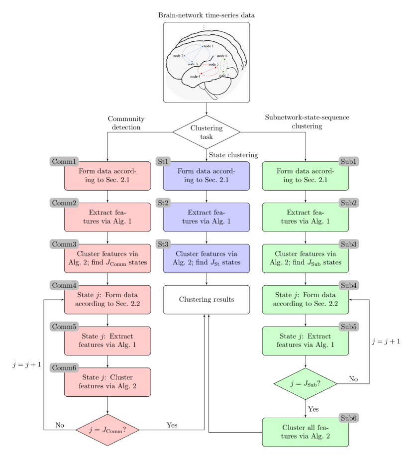
Figure 2: The pipeline of the proposed clustering framework.

For convenience, the proposed clustering framework is summarized in Fig. 2, and its building blocks, or modules, are delineated in the rest of the paper. The K-ARMA model and the feature-extraction mechanism are introduced in Section 2. The new variant of the GCT clustering algorithm is presented in Section 3, while numerical tests on synthetic and real fMRI data are showed in Section 4. Numerical tests and results that do not fit in the main manuscript are deferred to the supplementary file. Sections, figures, and tables of the supplementary manuscript are marked with the “S” qualifier.

2 Network-Feature Extraction by Kernel-ARMA Modeling

Consider a (brain) network/graph $\mathcal{G}\coloneqq(\mathcal{N},\mathcal{E})$, with sets of nodes $\mathcal{N}$, of cardinality $\lvert\mathcal{N}\rvert$, and edges $\mathcal{E}$. Each node $\nu\in\mathcal{N}$ is annotated with a stochastic process (time series) $(\prescript{}{\nu}{y}_{t})_{t\in\mathbb{Z}}$, where $t$ denotes discrete time and $\mathbb{Z}$ the set of all integer numbers; cf. Fig. 1. To avoid congestion in notations, $\prescript{}{\nu}{y}_{t}$ stands for both the random variable (RV) and its realization. In fMRI, nodes $\mathcal{N}$ comprise regions of interest (ROI) of the brain which are created either anatomically or functionally, and $(\prescript{}{\nu}{y}_{t})_{t\in\mathbb{Z}}$ becomes a blood-oxygen-level dependent (BOLD) time series [29], e.g., Fig. 4e. For index $\mathcal{V}\subset\mathcal{N}$ and $q\in\mathbb{Z}_{>0}$, the $q\times 1$ vector $\prescript{}{\mathcal{V}}{\mathbf{y}}_{t}$ is used in this manuscript to collect all signal samples from node(s) $\mathcal{V}$ of the network at time $t$, and to unify several scenarios of interest as the following discussion demonstrates.

2.1 State Clustering ($\mathcal{V}\coloneqq\mathcal{N}$)

Since a “state” is a global attribute of the network, vector $\prescript{}{\mathcal{N}}{\mathbf{y}}_{t}\coloneqq[\prescript{}{1}{y}_{t},\ldots,\prescript{}{\lvert\mathcal{N}\rvert}{y}_{t}]^{\intercal}$, with $\mathcal{V}\coloneqq\mathcal{N}$ and $q\coloneqq\lvert\mathcal{N}\rvert$, stands as the "snapshot" of the network at time $t$. The time series $(\prescript{}{\mathcal{N}}{\mathbf{y}}_{t})_{t}$ are the data formed in modules St1, Comm1 and Sub1 of Fig. 2.

2.2 Community Detection and Subnetwork-State-Sequence Clustering ($\mathcal{V}\coloneqq\nu$)

In the case of community detection and subnetwork-state-sequence clustering, nodes $\mathcal{N}$ need to be partitioned through the (dis)similarities of their time series. To detect common features and to identify those nodes, it is desirable first to extract individual features from each nodal time series. To this end, $\mathcal{V}$ is assigned the value $\nu$, so that $\forall\nu\in\mathcal{N}$, for a given buffer length $\texttt{Buff}_{\nu}\in\mathbb{Z}_{>0}$ and with $q=\texttt{Buff}_{\nu}$, $\prescript{}{\nu}{\mathbf{y}}_{t}$ takes the form of $[\prescript{}{\nu}{y}_{t},\ldots,\prescript{}{\nu}{y}_{t+\texttt{Buff}_{\nu}-1}]^{\intercal}$. If $\mathfrak{T}_{j}$ comprises all time indices of the $j$th state of a network, then the time series $\{(\prescript{}{\nu}{\mathbf{y}}_{t})_{t\in\mathfrak{T}_{j}}\}_{\nu\in\mathcal{N}}$ are the data formed in modules Comm4 and Sub4 of Fig. 2.

2.3 Extracting Grassmannian Features

Consider now a user-defined RKHS $\mathcal{H}$ with its kernel mapping $\varphi(\cdot)$; cf. Sec. A. Given $N\in\mathbb{Z}_{>0}$ and assuming that the sequence $(\prescript{}{\mathcal{V}}{\mathbf{y}}_{t})_{t}$ is available, define $\bm{\varphi}_{t}\coloneqq[\varphi(\prescript{}{\mathcal{V}}{\mathbf{y}}_{t}),\varphi(\prescript{}{\mathcal{V}}{\mathbf{y}}_{t+1}),\ldots,\varphi(\prescript{}{\mathcal{V}}{\mathbf{y}}_{t+N-1})]^{\intercal}\in\mathcal{H}^{N}$. This work proposes the following kernel (K-)ARMA model to fit the variations of features $\{\bm{\varphi}_{t}\}_{t}$ within space $\mathcal{H}^{N}$: There exist matrices $\mathbf{C}\in\mathbb{R}^{N\times\rho}$, $\mathbf{A}\in\mathbb{R}^{\rho\times\rho}$, the latent variable $\bm{\psi}_{t}\in\mathcal{H}^{\rho}$, and vectors $\bm{\upsilon}_{t}\in\mathcal{H}^{N}$, $\bm{\omega}_{t}\in\mathcal{H}^{\rho}$ that capture noise and approximation errors, s.t. $\forall t$,

$$\bm{\varphi}_{t} =\mathbf{C}\bm{\psi}_{t}+\bm{\upsilon}_{t}\,,$$ (1a)

$$\bm{\psi}_{t} =\mathbf{A}\bm{\psi}_{t-1}+\bm{\omega}_{t}\,.$$ (1b)

Kernel-based ARMA models have been already studied in the context of support-vector regression [30, 31, 32]. However, those models are different than (1) since only the AR and MA vectors of coefficients are mapped to an RKHS feature space, while the observed data $\prescript{}{\nu}{y}_{t}$ (of only a single time series) are kept in the input space. Here, (1) offers a way to map even the observed data to an RKHS to capture non-linearities in data via applying the ARMA idea to properly chosen feature spaces. In a different context [33], time series of graph-distance metrics are fitted by ARMA modeling to detect anomalies and thus identify states in networks. Neither the Grassmannian nor kernel functions were investigated in [33].

Proposition 1.

Given parameter $m\in\mathbb{Z}_{>0}$, define the “forward” matrix-valued function

$$\bm{\mathcal{F}}_{t} \coloneqq\begin{bmatrix}\bm{\varphi}_{t}&\bm{\varphi}_{t+1}&\ldots&\bm{\varphi}_{t+\tau_{\text{f}}-1}\\ \bm{\varphi}_{t+1}&\bm{\varphi}_{t+2}&\ldots&\bm{\varphi}_{t+\tau_{\text{f}}}\\ \vdots&\vdots&\ddots&\vdots\\ \bm{\varphi}_{t+m-1}&\bm{\varphi}_{t+m}&\ldots&\bm{\varphi}_{t+\tau_{\text{f}}+m-2}\end{bmatrix}\in\mathcal{H}^{mN\times\tau_{\text{f}}}\,,$$ (2a)

and the “backward” matrix-valued function

$$\bm{\mathcal{B}}_{t} \coloneqq\begin{bmatrix}\bm{\varphi}_{t}&\bm{\varphi}_{t+1}&\ldots&\bm{\varphi}_{t+\tau_{\text{f}}-1}\\ \bm{\varphi}_{t-1}&\bm{\varphi}_{t}&\ldots&\bm{\varphi}_{t+\tau_{\text{f}}-2}\\ \vdots&\vdots&\ddots&\vdots\\ \bm{\varphi}_{t-\tau_{\text{b}}+1}&\bm{\varphi}_{t-\tau_{\text{b}}+2}&\ldots&\bm{\varphi}_{t+\tau_{\text{f}}-\tau_{\text{b}}}\end{bmatrix}\in\mathcal{H}^{\tau_{\text{b}}N\times\tau_{\text{f}}}\,.$$ (2b)

Then, there exist matrices $\bm{\Pi}_{t+1}\in\mathbb{R}^{\rho\times\tau_{\text{b}}N}$ and $\bm{\mathcal{E}}_{t+1}^{\tau_{\text{f}}}\in\mathbb{R}^{mN\times\tau_{\text{b}}N}$ s.t. the following low-rank factorization holds true:

$$\tfrac{1}{\tau_{\text{f}}}\bm{\mathcal{F}}_{t+1}\operatorname{\otimes_{\mathcal{H}}}\bm{\mathcal{B}}_{t}^{\intercal}=\mathbf{O}\bm{\Pi}_{t+1}+\bm{\mathcal{E}}_{t+1}^{\tau_{\text{f}}}\,,$$ (3)

where product $\operatorname{\otimes_{\mathcal{H}}}$ is defined in Sec. A, and $\mathbf{O}$ is the so-called observability matrix: $\mathbf{O}\coloneqq\left[\mathbf{C}^{\intercal},(\mathbf{CA})^{\intercal},\ldots,(\mathbf{CA}^{m-1})^{\intercal}\right]^{\intercal}\in\mathbb{R}^{mN\times\rho}$.

With regards to a probability space, if (i) $(\bm{\upsilon}_{t})_{t}$and $(\bm{\omega}_{t})_{t}$ in (1) are considered to be zero-mean, independent and identically distributed stochastic processes, as well as independent of each other, (ii) $(\bm{\omega}_{t})_{t}$is independent of $(\bm{\psi}_{t})_{t}$, and (iii) $\bm{\omega}_{t}$and $\bm{\psi}_{t^{\prime}}$, $\forall(t,t^{\prime})$ s.t. $t>t^{\prime}$, are independent, then

$$\operatorname{\mathbb{E}}\left\{\tfrac{1}{\tau_{\text{f}}}\bm{\mathcal{F}}_{t+1}\operatorname{\otimes_{\mathcal{H}}}\bm{\mathcal{B}}_{t}^{\intercal}\nonscript\,\middle|\allowbreak\nonscript\,\mathopen{}\{\bm{\psi}_{t^{\prime}}\}_{t^{\prime}=t-\tau_{\text{b}}+1}^{t+\tau_{\text{f}}+m-1}\right\}=\mathbf{O}\bm{\Pi}_{t+1}\,.$$ (4)

If, in addition, (iv) $(\bm{\omega}_{t})_{t}$, $(\bm{\upsilon}_{t})_{t}$, $(\bm{\psi}_{t})_{t}$, and $(\bm{\omega}_{t}\operatorname{\otimes_{\mathcal{H}}}\bm{\psi}_{t-\tau}^{\intercal})_{t}$, $\forall\tau\in\mathbb{Z}_{>0}$, are wide-sense stationary, then $\lim_{\tau_{\text{f}}\to\infty}\bm{\mathcal{E}}_{t}^{\tau_{\text{f}}}=\mathbf{0}$, $\forall t$, in the mean-square ($\mathcal{L}_{2}$-) sense w.r.t. the probability space.

Proof of Proposition 1 1.

See B.

Motivated by (3) and (4), the result ($\lim_{\tau_{\text{f}}\to\infty}\bm{\mathcal{E}}_{t}^{\tau_{\text{f}}}=\mathbf{0}$, $\forall t$), and the fact that the conditional expectation is the least-squares-best estimator [34, §9.4], the following task is proposed to obtain an estimate of the observability matrix:

$$\left(\prescript{}{\mathcal{V}}{\hat{\mathbf{O}}}_{t},\hat{\bm{\Pi}}_{t}\right)\in\operatorname*{arg\,min}_{\begin{subarray}{c}\mathbf{O}\in\mathbb{R}^{mN\times\rho}\\ \bm{\Pi}\in\mathbb{R}^{\rho\times\tau_{\text{b}}N}\end{subarray}}\left\lVert\tfrac{1}{\tau_{\text{f}}}\bm{\mathcal{F}}_{t+1}\operatorname{\otimes_{\mathcal{H}}}\bm{\mathcal{B}}_{t}^{\intercal}-\mathbf{O}\bm{\Pi}\right\rVert_{\text{F}}^{2}\,.$$ (5)

To solve (5), the singular value decomposition (SVD) is applied to obtain $(1/\tau_{\text{f}})\bm{\mathcal{F}}_{t+1}\operatorname{\otimes_{\mathcal{H}}}\bm{\mathcal{B}}_{t}^{\intercal}=\mathbf{U}\bm{\Sigma}\mathbf{V}^{\intercal}$, where $\mathbf{U}\in\mathbb{R}^{mN\times mN}$ is orthogonal. Assuming that $\rho\leq\operatorname{rank}[(1/\tau_{\text{f}})\bm{\mathcal{F}}_{t+1}\operatorname{\otimes_{\mathcal{H}}}\bm{\mathcal{B}}_{t}^{\intercal}]$, the Schmidt-Mirsky-Eckart-Young theorem [35] provides the estimates $\prescript{}{\mathcal{V}}{\hat{\mathbf{O}}}_{t}\coloneqq\mathbf{U}_{:,1:\rho}$ and $\hat{\bm{\Pi}}_{t}\coloneqq\bm{\Sigma}_{1:\rho,1:\rho}\mathbf{V}^{\intercal}_{:,1:\rho}$, where $\mathbf{U}_{:,1:\rho}$ is the orthogonal matrix that collects those columns of $\mathbf{U}$ that correspond to the top (principal) $\rho$ singular values in $\bm{\Sigma}$.

Due to the factorization $\mathbf{O}\bm{\Pi}$, identifying the observability matrix becomes ambiguous, since for any non-singular matrix $\mathbf{P}\in\mathbb{R}^{\rho\times\rho}$, $\mathbf{O}\bm{\Pi}=\mathbf{O}\mathbf{P}\cdot\mathbf{P}^{-1}\bm{\Pi}$, and $\prescript{}{\mathcal{V}}{\hat{\mathbf{O}}}_{t}\mathbf{P}$ can serve also as an estimate. By virtue of the elementary observation that the column (range) spaces of $\prescript{}{\mathcal{V}}{\hat{\mathbf{O}}}_{t}\mathbf{P}$ and $\prescript{}{\mathcal{V}}{\hat{\mathbf{O}}}_{t}$ coincide, it becomes preferable to identify the column space of $\prescript{}{\mathcal{V}}{\hat{\mathbf{O}}}_{t}$, denoted hereafter by $[\prescript{}{\mathcal{V}}{\hat{\mathbf{O}}}_{t}]$, rather than the matrix $\prescript{}{\mathcal{V}}{\hat{\mathbf{O}}}_{t}$ itself. If $\rho=\operatorname{rank}[\prescript{}{\mathcal{V}}{\hat{\mathbf{O}}}_{t}]$, then $[\prescript{}{\mathcal{V}}{\hat{\mathbf{O}}}_{t}]$ becomes a point in the Grassmann manifold $\text{Gr}(\rho,mN)$, or Grassmannian, which is defined as the collection of all linear subspaces of $\mathbb{R}^{mN}$ with rank equal to $\rho$ [36, p. 73]. The Grassmannian $\text{Gr}(\rho,mN)$ is a Riemannian manifold with dimension equal to $\rho(mN-\rho)$ [36, p. 74]. The algorithmic procedure of extracting the feature $[\prescript{}{\mathcal{V}}{\hat{\mathbf{O}}}_{t}]$ from the available data is summarized in Alg. 1. To keep notation as general as possible, instead of using all of the signal samples, a subset $\mathfrak{T}\subset\mathbb{Z}$ is considered and signal samples are gathered in $(\prescript{}{\nu}{y}_{t})_{t\in\mathfrak{T}}$ per node $\nu$.

1

Parameters : Time indices $\mathfrak{T}$, and positive integers $N$, $m$, $\rho$, $\tau_{\text{f}}$, $\tau_{\text{b}}$.

2

Input : Time series $(\prescript{}{\mathcal{V}}{\mathbf{y}}_{t})_{t\in\mathfrak{T}}$.

3

Output : Grassmannian features $\{x_{t}\}_{t\in\mathfrak{T}}$.

4

5for all $t\in\mathfrak{T}$ do

6      

7      Form $(1/\tau_{\text{f}})\bm{\mathcal{F}}_{t+1}\operatorname{\otimes_{\mathcal{H}}}\bm{\mathcal{B}}_{t}^{\intercal}$ via (2).

8      Apply SVD: $(1/\tau_{\text{f}})\bm{\mathcal{F}}_{t+1}\operatorname{\otimes_{\mathcal{H}}}\bm{\mathcal{B}}_{t}^{\intercal}=\mathbf{U}\bm{\Sigma}\mathbf{V}^{\intercal}$.

9      Feature $x_{t}\coloneqq[\prescript{}{\mathcal{V}}{\hat{\mathbf{O}}}_{t}]\in\text{Gr}(\rho,mN)$ is the linear subspace spanned by the $\rho$ “principal” columns of $\mathbf{U}$.

10

Algorithm 1 Extracting Grassmannian features

There can be many choices for the reproducing kernel function $\kappa(\cdot,\cdot)$ (cf. Sec. A). If the linear kernel $\kappa_{\text{lin}}$ is chosen, then $\mathcal{H}=\mathbb{R}^{q}$, $\varphi(\cdot)$ becomes the identity mapping, $\bm{\varphi}_{t}=[\mathbf{y}_{t}^{\intercal},\mathbf{y}_{t+1}^{\intercal},\ldots,\mathbf{y}_{t+N-1}^{\intercal}]^{\intercal}\in\mathbb{R}^{qN}$, and $\operatorname{\otimes_{\mathcal{H}}}$ boils down to the usual matrix product. This case was introduced in [24]. The most popular choice for $\kappa$ is the Gaussian kernel $\kappa_{\text{G};\sigma}$, where parameter $\sigma>0$ stands for standard deviation. However, pinpointing the appropriate $\sigma_{*}$ for a specific dataset is a difficult task which may entail cumbersome cross-validation procedures [37]. A popular approach to circumvent the judicious selection of $\sigma_{*}$ is to use a dictionary of parameters $\{\sigma_{j}\}_{j=1}^{J}$, with $J\in\mathbb{Z}_{>0}$, to cover an interval where $\sigma_{*}$ is known to belong to. A reproducing kernel function $\kappa(\cdot,\cdot)$ can be then defined as the convex combination $\kappa(\cdot,\cdot)\coloneqq\sum_{j=1}^{J}\gamma_{j}\kappa_{\text{G};\sigma_{j}}(\cdot,\cdot)$, where $\{\gamma_{j}\}_{j=1}^{J}$ are convex weights, i.e., non-negative real numbers s.t. $\sum_{j=1}^{J}\gamma_{j}=1$ [37]. Such a strategy is followed in Section 4. Examples of non-Gaussian kernels can be also found in Sec. A.

Parameters in Alg. 1 need to be chosen properly to guarantee that features $\{x_{i}\}_{i\in\mathfrak{I}}$ capture the statistical information of the time series. Parameters $N$, $m$ and $\rho$ control the dimension $\rho(mN-\rho)$ of the Grassmannian, which should be large enough to capture the variability of the assumed low-dimensional feature point-cloud. The sum $m+\tau_{\text{f}}+\tau_{\text{b}}$ should not be greater than the length of the time series due to the size of "forward" and "backward’ matrices $\bm{\mathcal{F}}_{t}$ and $\bm{\mathcal{B}}_{t}$, while large values of $\tau_{\text{f}}$ can help in reducing the estimation error of ${\prescript{}{\mathcal{V}}{\hat{\mathbf{O}}}}_{t}$.

3 Network Clustering In The Grassmannian

3.1 Extended Geodesic Clustering by Tangent Spaces

Having extracted and mapped features into the Grassmannian, the next task in the pipeline of the framework is clustering. To keep this module as generic as possible, the index set $\mathfrak{I}$ will be used henceforth to mark features in $\{x_{i}\}_{i\in\mathfrak{I}}$.

This work follows the Riemannian multi-manifold modeling (RMMM) hypothesis [27, 26, 24], where clusters $\{\mathcal{C}_{k}\}_{k=1}^{K}$ are considered to be submanifolds of the Grassmannian, and data $\{x_{i}\}_{i}$ are located close to or onto $\{\mathcal{C}_{k}\}_{k=1}^{K}$ (see Fig. 3a for the case of $K=2$ clusters). RMMM allows for clusters to intersect; a case where the classical K-means, for example, is known to face difficulties [38].

Clustering is performed by Alg. 2, coined geodesic clustering by tangent spaces (GCT). The present GCT extends its initial form of [27, 26, 24] to the case of Alg. 2 where there is no need to know the number $K$ of clusters a-priori. This desirable feature of Alg. 2 is also along the lines of usual practice, where it is unrealistic to know $K$ before employing a clustering algorithm.

In a nutshell, Alg. 2 computes the affinity matrix $\mathbf{W}$ of features $\{x_{i}\}_{i\in\mathfrak{I}}$ in step 2, comprising information about sparse data approximations, via weights $\{\alpha_{ii^{\prime}}\}_{i,i^{\prime}\in\mathfrak{I}}$, as well as the angular information $\{\theta_{ii^{\prime}}\}_{i,i^{\prime}\in\mathfrak{I}}$. Although the incorporation of sparse weights originates from [39], one of the novelties of GCT is the usage of the angular information via $\{\theta_{ii^{\prime}}\}_{i,i^{\prime}\in\mathfrak{I}}$. GCT’s version of [27, 26, 24] applies spectral clustering in step 2, where knowledge of the number of clusters $K$ is necessary. To surmount the obstacle of knowing $K$ beforehand, Louvain clustering method [40] is adopted in step 2. The Louvain method belongs to the family of hierarchical-clustering algorithms that attempt to maximize a modularity function, which monitors the intra- and inter-cluster density of links/edges. Needless to say that any other hierarchical-clustering scheme can be used at step 2 instead of Louvain method.

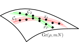
(a) Clusters on $\text{Gr}(\rho,mN)$

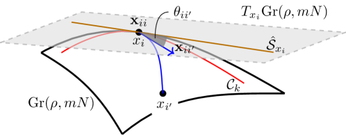
(b) Angular information

Figure 3: (a) The Riemannian multi-manifold modeling (RMMM) hypothesis. (b) Angular information computed in tangent spaces and used in Alg. 2.

1

Input : Grassmannian features $\{x_{i}\}_{i\in\mathfrak{I}}$.

2

Parameters : $K_{\text{NN}}\in\mathbb{Z}_{>0}$ and $\sigma_{\alpha},\sigma_{\theta}\in\mathbb{R}_{>0}$.

3

Output : Clusters $\{\mathcal{C}_{k}\}_{k=1}^{K}$.

4

5for all $i\in\mathfrak{I}$ do

6      

7      Define the $K_{\text{NN}}$-nearest-neighbors $\mathscr{N}_{\text{NN}}(x_{i})$.

8      Map $\mathscr{N}_{\text{NN}}(x_{i})$ into the tangent space $T_{x_{i}}\text{Gr}(\rho,mN)$ of the Grassmannian at $x_{i}$ via the logarithm map: $\mathbf{x}_{ii^{\prime}}\coloneqq\log_{x_{i}}(x_{i^{\prime}})$, $\forall x_{i^{\prime}}\in\mathscr{N}_{\text{NN}}(x_{i})$.

9      Identify $\{\alpha_{ii^{\prime}}\}_{x_{i^{\prime}}\in\mathscr{N}_{\text{NN}}(x_{i})}$ via (6). Set $\alpha_{ii^{\prime}}\coloneqq 0$, for all $i^{\prime}$ s.t. $x_{i^{\prime}}\notin\mathscr{N}_{\text{NN}}(x_{i})$.

10      Compute the sample correlation matrix $\hat{\mathbf{C}}_{x_{i}}$ in (7).

11      Perform principal component analysis (PCA) on $\hat{\mathbf{C}}_{x_{i}}$ to extract the eigenspace $\hat{\mathcal{S}}_{x_{i}}$.

12      Compute angle $\theta_{ii^{\prime}}$ between vector $\mathbf{x}_{ii^{\prime}}-\mathbf{x}_{ii}$ and $\hat{\mathcal{S}}_{x_{i}}$, $\forall x_{i^{\prime}}\in\mathscr{N}_{\text{NN}}(x_{i})$ (${\theta_{ii}}\coloneqq 0$). Let also $\theta_{ii^{\prime}}\coloneqq 0$ for $x_{i^{\prime}}\notin\mathscr{N}_{\text{NN}}(x_{i})$.

13

14Form the symmetric $\lvert\mathfrak{I}\rvert\times\lvert\mathfrak{I}\rvert$ affinity (adjacency) matrix $\mathbf{W}\coloneqq[w_{ii^{\prime}}]_{(i,i^{\prime})\in\mathfrak{I}^{2}}$, where entry $w_{ii^{\prime}}$ is defined as

$$w_{ii^{\prime}}\coloneqq\exp(\lvert\alpha_{ii^{\prime}}\rvert+\lvert\alpha_{i^{\prime}i}\rvert)\cdot\exp[-(\theta_{ii^{\prime}}+\theta_{i^{\prime}i})/\sigma_{\theta}]\,.$$

15Apply Louvain method [40] to $\mathbf{W}$ to parcellate the data $(x_{i})_{i\in\mathfrak{I}}$ into clusters $\{\mathcal{C}_{k}\}_{k=1}^{K}$.

Algorithm 2 Extended geodesic clustering by tangent spaces (eGCT)

A short description of the steps in Alg. 2 follows, with Riemannian-geometry details deferred to [27, 26, 24]. Alg. 2 visits $\{x_{i}\}_{i\in\mathfrak{I}}$ sequentially (step 2). At step 2, the $K_{\text{NN}}$-nearest-neighbors $\mathscr{N}_{\text{NN}}(x_{i})$ of $x_{i}$ are identified, i.e., those $K_{\text{NN}}$ points, taken from $\{x_{i}\}_{i}$, which are placed the closest from $x_{i}$ with respect to the Grassmannian distance [41]. The neighbors $\mathscr{N}_{\text{NN}}(x_{i})$ are then mapped at step 2 to the Euclidean vectors $\{\mathbf{x}_{ii^{\prime}}\}_{x_{i^{\prime}}\in\mathscr{N}_{\text{NN}}(x_{i})}$ in the tangent space $T_{x_{i}}\text{Gr}(\rho,mN)$ of the Grassmannian at $x_{i}$ (the gray-colored plane in Fig. 3b) via the logarithm map $\log_{x_{i}}(\cdot)$, whose computation (non-closed form via SVD) is provided in [27, 24]. Step 2 computes the weights $\{\alpha_{ii^{\prime}}\}_{x_{i^{\prime}}\in\mathscr{N}_{\text{NN}}(x_{i})}$, with $\alpha_{ii}\coloneqq 0$, via the following sparse-coding task:

$$\min_{\{\alpha_{ii^{\prime}}\}}{} {}\left\lVert\mathbf{x}_{ii}-\sum\nolimits_{x_{i^{\prime}}\in\mathscr{N}_{\text{NN}}(x_{i})\setminus\{x_{i}\}}\alpha_{ii^{\prime}}\mathbf{x}_{ii^{\prime}}\right\rVert^{2}$$

$${}+\sum\nolimits_{x_{i^{\prime}}\in\mathscr{N}_{\text{NN}}(x_{i})\setminus\{x_{i}\}}\exp[{\lVert\mathbf{x}_{ii^{\prime}}-\mathbf{x}_{ii}\rVert/\sigma_{\alpha}}]\cdot|\alpha_{ii^{\prime}}|$$

s.to $${}\sum\nolimits_{x_{i^{\prime}}\in\mathscr{N}_{\text{NN}}(x_{i})\setminus\{x_{i}\}}\alpha_{ii^{\prime}}=1\,.$$ (6)

The affine constraint in (6), imposed on the $\{\alpha_{ii^{\prime}}\}$ coefficients in representing $\mathbf{x}_{ii}$ via its neighbors, is motivated by the affine nature of the tangent space (Fig. 3b). Moreover, the larger the distance of neighbor $\mathbf{x}_{ii^{\prime}}$ from $\mathbf{x}_{ii}$, the larger the weight $\exp[{\lVert\mathbf{x}_{ii^{\prime}}-\mathbf{x}_{ii}\rVert/\sigma_{\alpha}}]$, which in turn penalizes severely the coefficient $\alpha_{ii^{\prime}}$ by pushing it to values close to zero. Step 2 computes the sample covariance matrix

$$\hat{\mathbf{C}}_{x_{i}}\coloneqq\tfrac{1}{\lvert\mathscr{N}_{\text{NN}}(x_{i})\rvert-1}\sum\nolimits_{x_{i^{\prime}}\in\mathscr{N}_{\text{NN}}(x_{i})}(\mathbf{x}_{ii^{\prime}}-\bar{\mathbf{x}}_{i})(\mathbf{x}_{ii^{\prime}}-\bar{\mathbf{x}}_{i})^{\intercal}\,,$$ (7)

where $\bar{\mathbf{x}}_{i}\coloneqq(1/\lvert\mathscr{N}_{\text{NN}}(x_{i})\rvert)\sum_{x_{i^{\prime}}\in\mathscr{N}_{\text{NN}}(x_{i})}\mathbf{x}_{ii^{\prime}}$ denotes the sample average of the neighbors of $\mathbf{x}_{ii}$. PCA is applied to $\hat{\mathbf{C}}_{x_{i}}$ at step 2 to compute the principal eigenspace $\hat{S}_{x_{i}}$, which may be viewed as an approximation of the image of the cluster (submanifold) $\mathcal{C}_{k}$, via the logarithm map, into the tangent space $T_{x_{i}}\text{Gr}(\rho,mN)$ (see Fig. 3b). Once $\hat{S}_{x_{i}}$ is computed, the angle $\theta_{ii^{\prime}}$ between vector $\mathbf{x}_{ii^{\prime}}-\mathbf{x}_{ii}$ and $\hat{\mathcal{S}}_{x_{i}}$ is also computed at step 2 to extract angular information. The larger the angle $\theta_{ii^{\prime}}$ is, the less the likelihood for $x_{i^{\prime}}$ to belong to cluster $\mathcal{C}_{k}$. The additional use of angular information by GCT advances the boundary of state-of-the-art clustering methods in the Grassmannian, where, usually, the weights of the adjacency matrix are defined via the Grassmannian (geodesic) distance or sparse-coding schemes [39].

3.2 Summarizing the Network-Clustering Framework

To summarize, the flowchart of the network-clustering framework is presented in Fig. 2. The most straightforward path is the (blue-colored) state-clustering one, where data are firstly formed (St1), then Alg. 1 is applied to those data to collect features (St2), and finally Alg. 2 is utilized to assign those features into clusters $\{\mathcal{C}_{k}\}_{k=1}^{K}$ (St3). In this context, clustering is equivalent to parcellating the time horizon $\mathfrak{T}$ into a partition $\{\mathfrak{T}_{j}\}_{j=1}^{J}$ of time intervals s.t. data $(\prescript{}{\lvert\mathcal{N}\rvert}{y}_{t})_{t\in\mathfrak{T}_{j}}$ are mapped to the same state $j$.

The “community-detection” (red color) and “subnetwork-state-sequence-clustering” (green color) paths require state clustering as a pre-processing part. This is necessary in order to achieve high accuracy clustering results. Without knowing the starting and ending points of different states, there will be time-series vectors $\prescript{}{\nu}{\mathbf{y}}_{t}$ in Alg. 1 which capture data from two consecutive states, since $\prescript{}{\nu}{\mathbf{y}}_{t}$ takes the form of $[\prescript{}{\nu}{y}_{t},\ldots,\prescript{}{\nu}{y}_{t+\texttt{Buff}_{\nu}-1}]^{\intercal}$. Features corresponding to those vectors will decrease the clustering accuracy since the extracted features do not correspond to any actual state or community. Once states are determined, the features that come from two consecutive states are ignored and the time horizon $\mathfrak{T}$ is partitioned in $\{\mathfrak{T}_{j}\}_{j=1}^{J}$, then Algs. 1 and 2 are applied per state $j$ to detect communities (Comm4–Comm6). In “subnetwork-state-sequence clustering,” states are again identified first. Per state, nodal time-series data are formed according to Sec. 2.2 (Sub4) and nodal features are extracted by Alg. 1 (Sub5). All those features from all states are collected and finally Alg. 2 is applied to track/identify subnetwork state sequences (Sub6).

3.3 Computational Complexity

The main computational burden comes from the feature extracting and clustering steps in Alg. 1 and Alg. 2. If $\mathfrak{I}$ denotes the points in the Grassmannian, the computational complexity for computing features $\{x_{i}\}_{i\in\mathfrak{I}}$ in Alg. 1 is $\mathcal{O}(|\mathfrak{I}|\mathcal{C}_{\operatorname{\otimes_{\mathcal{H}}}})$, where $\mathcal{C}_{\operatorname{\otimes_{\mathcal{H}}}}$ denotes the cost of computing $\bm{\mathcal{F}}_{t+1}\operatorname{\otimes_{\mathcal{H}}}\bm{\mathcal{B}}_{t}^{\intercal}$, which includes SVD computations. In Alg. 2, the complexity for computing the $\mathscr{N}_{\text{NN}}(x_{i})$ nearest neighbors of $x_{i}$ is $\mathcal{O}(|\mathfrak{I}|\mathcal{C}_{\text{dist}}+\mathscr{N}_{\text{NN}}\log|\mathfrak{I}|)$, where $\mathcal{C}_{\text{dist}}$ denotes the cost of computing the Riemannian distance between any two points, and $\mathscr{N}_{\text{NN}}\log|\mathfrak{I}|$ refers to the cost of finding the $\mathscr{N}_{\text{NN}}$ nearest neighbors of $x_{i}$. Step 2 of Alg. 2 is a sparsity-promoting optimization task of (6) and let $\mathcal{C}_{\text{SC}}$ denotes the complexity to solve it. Under $\mathcal{M}\coloneqq\text{Gr}(\rho,mN)$, step 2 of Alg. 2 involves the computation of the eigenvectors of the sample covariance matrix $\hat{\mathbf{C}}_{x_{i}}$, with complexity of $\mathcal{O}(\dim\mathcal{M}+K_{\text{NN}}^{3})$. In step 2, the complexity for computing empirical geodesic angles is $\mathcal{O}[|\mathfrak{I}|(\mathcal{C}_{\log}+\dim\mathcal{M})]$, where $\mathcal{C}_{\log}$ is the complexity of computing the logarithm map $\log_{x_{i}}(\cdot)$; for details, see [24]. For the last step of Alg. 2, the exact complexity of Louvain method is not known but the method seems to run in time $\mathcal{O}(|\mathfrak{I}|\log|\mathfrak{I}|)$ with most of the computational effort spent on modularity optimization at first level, since modularity optimization is known to be NP-hard [42]. To summarize, the complexity of Alg. 2 is $\mathcal{O}[|\mathfrak{I}|^{2}(\mathcal{C}_{\text{dist}}+\mathcal{C}_{\log}+\dim\mathcal{M})+(K_{\text{NN}}+1)|\mathfrak{I}|\log|\mathfrak{I}|+|\mathfrak{I}|(\dim\mathcal{M}+K_{\text{NN}}^{3})]$.

4 Numerical Tests

This section validates the proposed framework on synthetic and real data. Tags eGCT[Sker] and eGCT[Mker] denote the proposed framework whenever a single and multiple kernel functions are employed, respectively. In the case where the linear kernel is used, the K-ARMA method boils down to the eGCT method of [24]. Apart from the classical K-means, other competing algorithms are: (i) The sparse manifold clustering and embedding (SMCE) [39]; (ii) interaction K-means with PCA (IKM-PCA) [43]; (iii) graph-shift-operator estimation (GOE) [20] from the popular graph-signal-processing framework; (iv) independent component analysis (ICA) [44, 45]; (v) multivariate Granger causality (MVGC) [46, 47]; (vi) 3D-windowed tensor approach (3D-WTA) [48]. More details are given in Sec. 5 of the supplementary file to abide by the thirty-pages limit for new paper submissions imposed by this journal. SMCE, 3D-WTA, ICA and the classical K-means will be compared against proposed framework on state clustering. SMCE, IKM-PCA, 3D-WTA, GOA, ICA, MVGC and K-means will be used in community detection. Since none of IKM-PCA, GOA, MVGC and 3D-WTA can perform subnetwork-state-sequence clustering across multiple states, only the results of proposed framework and SMCE are reported. To ensure fair comparisons, the parameters of all methods were tuned to reach optimal performance for every scenario at hand.

The evaluation of all methods was based on the following two criteria: (i) Clustering accuracy, defined as the number of correctly clustered data points (ground-truth labels are known) over the total number of points; (ii) normalized mutual information (NMI) [49]; and In what follows, every numerical value of the previous criteria is the uniform average of $20$ independently performed tests for the particular scenario at hand.

4.1 Synthetic Data

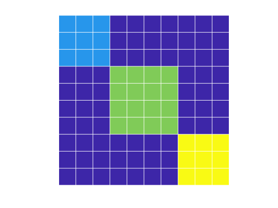
(a) State 1

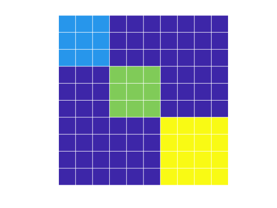
(b) State 2

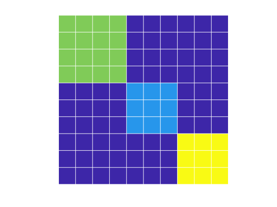
(c) State 3

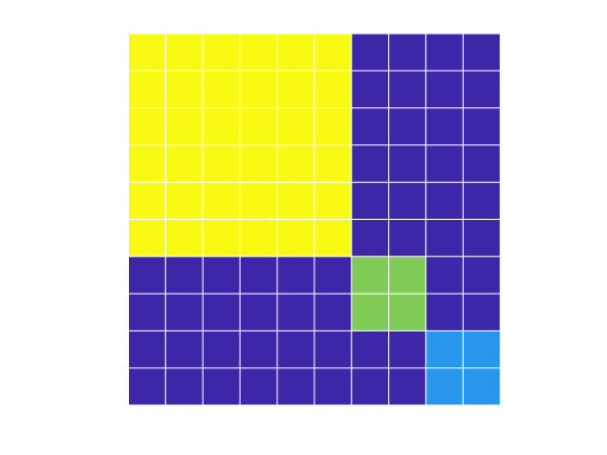
(d) State 4

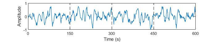
(e) BOLD time series of node #2, dataset #5

Figure 4: Synthetic data generated by the Matlab SimTB toolbox [44]. (a)-(d) Noiseless and outlier-free connectivity matrices corresponding to four network states. Nodes that share the same color cooperate to perform a common task.

Data were generated by the open-source Matlab SimTB toolbox [44]. A $10$-node network is considered that transitions successively between $4$ distinct network states. Every state corresponds to a certain connectivity matrix, generated via the following path. Each connectivity matrix, fed to the SimTB toolbox, is modeled as the superposition of three matrices: 1) The ground-truth (noiseless) connectivity matrix (cf. Fig. 4), where nodes sharing the same color belong to the same cluster and collaborate to perform a common task; 2) a symmetric matrix whose entries are drawn independently from a zero-mean Gaussian distribution with standard deviation $\sigma$ to model noise; and 3) a symmetric outlier matrix where $36$ entries are equal to $\mu$ to account for outlier neural activity.

Different states may share different outlier matrices, controlled by $\mu$. Aiming at extensive numerical tests, six datasets were generated (corresponding to the columns of Table 1) by choosing six pairs of parameters $(\mu,\sigma)$ in the modeling of the connectivity matrices and the SimTB toolbox. Datasets D1, D2 and D3 were created without outliers, while datasets D4, D5 and D6 include outlier matrices with different $\mu$s in different states. Table 6 details the parameters of those six datasets. Driven by the previous connectivity matrices, the SimTB toolbox generates BOLD time series [29]. Each state contributes $150$ signal samples, for a total of $4\times 150=600$ samples, to every nodal time series, e.g., Fig. 4e.

Table 1: Synthetic fMRI Data: State clustering

Methods	Without Outliers						With Outliers
	Clustering Accuracy			NMI			Clustering Accuracy			NMI
	D1	D2	D3	D1	D2	D3	D4	D5	D6	D4	D5	D6
eGCT	0.969	0.805	0.640	0.948	0.766	0.596	0.944	0.743	0.589	0.860	0.627	0.340
eGCT[Sker]	1	0.824	0.681	1	0.791	0.622	0.983	0.775	0.599	0.930	0.651	0.379
eGCT[Mker]	1	0.839	0.708	1	0.808	0.641	0.992	0.800	0.626	0.967	0.689	0.435
3DWTA [48]	1	0.792	0.603	1	0.735	0.556	0.943	0.731	0.517	0.872	0.562	0.281
SMCE [39]	0.920	0.784	0.583	0.887	0.673	0.480	0.883	0.712	0.508	0.713	0.558	0.246
ICA [44, 45]	0.943	0.734	0.527	0.821	0.605	0.364	0.926	0.719	0.474	0.795	0.533	0.215
Kmeans	0.866	0.670	0.402	0.800	0.560	0.307	0.768	0.621	0.337	0.476	0.403	0.168

Table 1 demonstrates the results of state clustering. The parameters used for eGCT, eGCT[Sker] and eGCT[Mker] are: $N\coloneqq 30$, $m\coloneqq 2$, $\rho\coloneqq 2$, $\tau_{f}\coloneqq 60$, $\tau_{b}\coloneqq 20$. The Gaussian kernel $\kappa_{\text{G};0.8}(\cdot,\cdot)$ (cf. Sec. A) is used in the single-kernel method eGCT[Sker], while kernel $\kappa(\cdot,\cdot)\coloneqq 0.6\,\kappa_{\text{G};0.8}(\cdot,\cdot)+0.4\,\kappa_{\text{L};1}(\cdot,\cdot)$ is used in the eGCT[Mker] case since it performed the best among other choices of kernel functions. Fig. 6 depicts also the standard deviations of the results of Table 1, computed after performing independent repetitions of the same test. To save space, the figures which include the standard deviations of the subsequent tests will be omitted.

Among all methods, eGCT[Mker] scores the highest clustering accuracy and NMI over all six datasets. It can be observed by Table 1 that the existence of outliers affects negatively the ability of all methods to cluster data. The main reason is that the algorithms tend to detect outliers and gather those in clusters different from the nominal ones. Ways to reject those outliers are outside of the scope of this study and will be provided in a future publication.

Table 2: Synthetic fMRI data: Community detection

Methods	Without Outliers						With Outliers
	Clustering Accuracy			NMI			Clustering Accuracy			NMI
	D1	D2	D3	D1	D2	D3	D4	D5	D6	D4	D5	D6
eGCT	1	0.960	0.842	1	0.876	0.775	0.973	0.910	0.817	0.940	0.793	0.664
eGCT[Sker]	1	1	0.915	1	1	0.838	1	0.942	0.852	1	0.864	0.710
eGCT[Mker]	1	1	0.945	1	1	0.907	1	0.958	0.879	1	0.892	0.803
3DWTA [48]	1	0.951	0.839	1	0.927	0.754	0.925	0.863	0.799	0.842	0.780	0.638
SMCE [39]	0.965	0.929	0.827	0.902	0.865	0.691	0.909	0.773	0.745	0.769	0.647	0.563
GOE [20]	1	0.933	0.809	1	0.915	0.655	0.918	0.740	0.684	0.833	0.652	0.409
ICA [44, 45]	0.974	0.936	0.830	0.917	0.883	0.702	0.910	0.826	0.761	0.828	0.715	0.592
MVGC [46, 47]	1	0.948	0.834	1	0.920	0.722	0.914	0.845	0.759	0.826	0.742	0.611
IKM-PCA [43]	0.948	0.907	0.791	0.890	0.814	0.629	0.892	0.756	0.712	0.738	0.551	0.486
Kmeans	0.908	0.876	0.725	0.810	0.729	0.547	0.843	0.672	0.605	0.620	0.391	0.314

Table 2 presents the results of community detection. The numerical values in Table 2 stand for the average values over the $4$ states for each one of the datasets. Parameters of eGCT, eGCT[Sker] and eGCT[Mker] were set as follows: $N\coloneqq 30$, $\texttt{Buff}_{\nu}\coloneqq 20$, $m\coloneqq 3$, $\rho\coloneqq 2$, $\tau_{f}\coloneqq 50$, $\tau_{b}\coloneqq 10$. In eGCT[Sker], the utilized kernel function is $\kappa_{\text{G};0.5}(\cdot,\cdot)$, while in eGCT[Mker] the kernel is defined as $\kappa(\cdot,\cdot)\coloneqq 0.5\,\kappa_{\text{G};0.5}(\cdot,\cdot)+0.5\,\kappa_{\text{L}0;1}(\cdot,\cdot)$ (cf. Sec. A). Table 2 demonstrates that eGCT[Mker] consistently outperforms all other methods across all datasets and even for the case where outliers contaminate the data. Fig. 7 depicts also the standard deviations of the results of Table 2.

Table 3: Synthetic fMRI data: Subnetwork state sequences

Methods	Without Outliers						With Outliers
	Clustering Accuracy			NMI			Clustering Accuracy			NMI
	D1	D2	D3	D1	D2	D3	D4	D5	D6	D4	D5	D6
eGCT	1	0.816	0.749	1	0.767	0.684	0.928	0.701	0.633	0.874	0.484	0.355
eGCT[Sker]	1	0.856	0.781	1	0.791	0.702	0.956	0.728	0.664	0.913	0.534	0.410
eGCT[Mker]	1	0.884	0.817	1	0.821	0.739	1	0.757	0.721	1	0.602	0.485
SMCE [39]	0.936	0.792	0.691	0.804	0.617	0.495	0.851	0.665	0.580	0.785	0.416	0.318

Table 3 illustrates the results of subnetwork-state-sequence clustering. The parameters of eGCT, eGCT[Sker] and eGCT[Mker] were set as follows: $N\coloneqq 20$, $\texttt{Buff}_{\nu}\coloneqq 50$, $m\coloneqq 3$, $\rho\coloneqq 3$, $\tau_{f}\coloneqq 45$, $\tau_{b}\coloneqq 5$. The kernel functions used in eGCT[Sker] and eGCT[Mker] are identical to those employed in Table 2. Similarly to the previous cases, eGCT[Mker] outperforms all other methods across all datasets and scenarios on both clustering accuracy and NMI. Fig. 8 depicts also the standard deviations of the results of Table 3.

4.2 Real Data

To validate the community detection framework,we tested our algorithm on functional networks derived for two subjects taken from the S1200 dataset of the Human Connectome Project (HCP) [50] were considered.

To avoid irrelevant influence, only the part of cleaned volume data in single run with left-to-right phase encoding direction was employed. In addition to the HCP preprocessing, each voxel was standardized by first subtracting the temporal mean and then applying global signal regression. Specifically, motion outliers was used to estimate framewise displacement (FD) [51] and volumes with FD>0.2 mm were censored and removed from further analysis. In addition, we standardized each voxel by first subtracting the temporal mean and then applying global signal regression. Brain regions were defined using either the standard 116 region AAL-atlas [52]. The temporal activity for a given brain region was computed by averaging the signal over all voxels within the region.

Table 4: Real fMRI data: community detection results

Community	Fitting rate
Cerebellum	0.381
Control	0.440
Default Mode	0.642
Dorsal Attention	0.422
Limbic	0.386
Salience/Ventral Attention	0.700
Somatomotor	0.554
Subcortical	0.357
Visual	0.633

Table 4 and Fig. 5 shows the community-detection results with 116 brain ROIs. Ten subjects are randomly selected from the HCP resting state fMRI data set. Nine cortical regions are considered as nine communities as labels of cognitive system. Each cortical region from the AAL atlas was mapped onto a cognitive system from the 7-Network parcellation scheme from the Schaefer-100 atlas, respectively [53]. Community label assignment was based on minimizing the Euclidian distance from the centroid of a region in the AAL to the corresponding Schaefer-100atlas over more than 1000 samples. Subcortical and Cerebellar regions were combined into their respective systems.

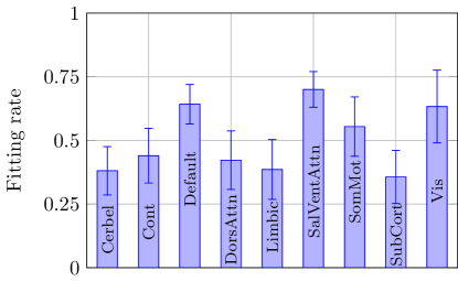
Figure 5: Real fMRI data : Community detection

Table 4 and Fig. 5 shows the community-detection results with 116 brain ROIs. Nodes/ROIs with the same color are in the same cluster. Ten samples are randomly selected from the data set. .

The state clustering results of real fMRI are briefly described in Sec. 7 of the supplementary file.

5 Supplementary: Competing Algorithms

5.1 Sparse Manifold Clustering and Embedding (SMCE) [39]

Each point on the Grassmannian is described by a sparse affine combination of its neighbors. The computed sparse weights define the entries of a similarity matrix, which is subsequently used to identify data-cluster associations. SMCE does not utilize any angular information, as step 2 of Alg. 2 does.

5.2 Interaction K-means with PCA (IKM-PCA) [43]

IKM is a clustering algorithm based on the classical K-means and Euclidean distances within a properly chosen feature space. To promote time-efficient solutions, the classical PCA is employed as a dimensionality-reduction tool for feature-subset selection. In this algorithm, the dimension of fMRI data is reduced by classical PCA first, then the PCA-processed data are clustered using IKM.

5.3 Graph-shift-operator estimation (GOE) [20]

The graph shift operator is a symmetric matrix capturing the network’s structure, i.e., topology. There are widely adopted choices of graph shift operators, including the adjacency and Laplacian matrices, or their various degree-normalized counterparts. An estimation algorithm in [20] computes the optimal graph shift operator via convex optimization. The computed graph shift operator is fed to a spectral-clustering module to identify communities within a single brain state, since [20] assumes stationary time-series data.

5.4 Independent Component Analysis based algorithms (ICA) [44, 45]

Independent component analysis discovers hidden features or factors from a set of observed data such that the discovered features are maximally independent. For state clustering, group ICA [44] is introduced. In this algorithm, features are extracted and examined for relationships among the data types at the group level (i.e., variations among time sliding windows, patients or controls). Then, functional connectivity matrices are estimated as covariance matrices and clustered by K-means. For community detection, [45] proposed a framework with ICA and hierarchical clustering to identify functional brain connectivity patterns of EEG and fMRI datasets.

5.5 Multivariate Granger causality (MVGC) [46, 47]

To explore the knowledge of functional brain network as well as connectivity patterns and community structures, multivariate Granger causality (MVGC) has recently been applied to incorporate information about the influence exerted by a brain region onto another. A MVGC toolbox is provided by [46] that estimates “Granger causality” and vector autoregressive coefficients on time or frequency domain of time series. A community detection framework based on MVGC toolbox is proposed in [47]. “Granger causality” strength between each pair of nodes/ROIs become the entries of an adjacency matrix, which is fed into spectral clustering for community detection.

5.6 3D-Windowed Tensor Approach (3D-WTA) [48]

3D-WTA was originally introduced for community detection in dynamic networks by applying tensor decompositions onto a sequence of adjacency matrices indexed over the time axis. 3D-WTA was modified in [21] to accommodate multi-layer network structures. High-order SVD (HOSVD) and high-order orthogonal iteration (HOOI) are used within a pre-defined sliding window to extract subspace information from the adjacency matrices. The “asymptotic-surprise” metric is used as the criterion to determine the number of clusters. 3D-WTA is capable of performing both state clustering and community detection.

6 Supplementary: Synthetic fMRI data

Table 6 provides the parameters $\mu$ and $\sigma$ used to generate noise matrices and symmetric matrices to simulate outlier neural activities. By choosing different combinations of $(\mu,\sigma)$, $6$ different synthetic fMRI datasets were created.

Table 5: Parameters $(\mu,\sigma)$ used to generate synthetic BOLD time series

o |X|X|X|X|X| $Dataset$	$State\ 1$	$State\ 2$	$State\ 3$	$State\ 4$
1	$(0,-10\text{dB})$	$(0,-10\text{dB})$	$(0,-10\text{dB})$	$(0,-10\text{dB})$
2	$(0,-8\text{dB})$	$(0,-8\text{dB})$	$(0,-8\text{dB})$	$(0,-8\text{dB})$
3	$(0,-6\text{dB})$	$(0,-6\text{dB})$	$(0,-6\text{dB})$	$(0,-6\text{dB})$
4	$(0.2,-10\text{dB})$	$(0.3,-10\text{dB})$	$(0.4,-10\text{dB})$	$(0.5,-10\text{dB})$
5	$(0.2,-8\text{dB})$	$(0.3,-8\text{dB})$	$(0.4,-8\text{dB})$	$(0.5,-8\text{dB})$
6	$(0.2,-6\text{dB})$	$(0.3,-6\text{dB})$	$(0.4,-6\text{dB})$	$(0.5,-6\text{dB})$

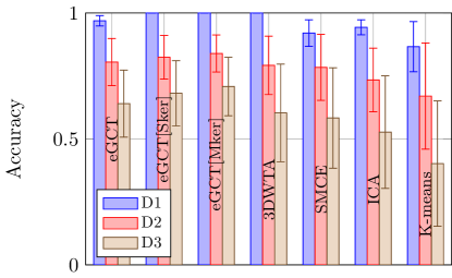
(a) Datasets 1, 2, 3

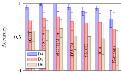
(b) Datasets 4, 5, 6

Figure 6: State-clustering results of synthetic fMRI datasets. (a) Data without an independent event; (b) Data with an independent event. These data sets are the same as D1, D2, etc, in Table 1.

Standard-deviation results of state clustering on synthetic fMRI datasets are demonstrated in Fig. 6. Standard deviation of all algorithms increase when the strength of the noisy matrix increases. For dataset D1, eGCT[Sker] , eGCT[Mker] and 3DWTA reach $100\%$ accuracy; for other datasets, eGCT[Mker] exhibits the highest accuracy and the smallest standard deviation.

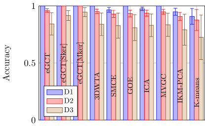
(a) Datasets 1, 2, 3

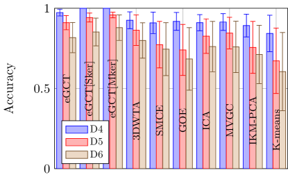
(b) Datasets 4, 5, 6

Figure 7: Community detection results of synthetic fMRI datasets. (a) Data without an independent event; (b) Data with an independent event. These data sets are the same as D1, D2, etc, in Table 2.

Fig. 7 illustrates the results of community detection for the synthetic fMRI datasets. eGCT, eGCT[Sker] , eGCT[Mker] and 3DWTA score $100\%$ accuracy for dataset D1, while eGCT[Sker] and eGCT[Mker] show $100\%$ accuracy for dataset D4. eGCT[Mker] shows the highest accuracy on all other datasets.

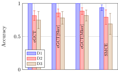
(a) Datasets 1, 2, 3

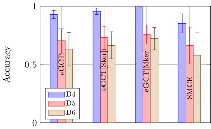
(b) Datasets 4, 5, 6

Figure 8: Subnetwork-state-sequence clustering results of synthetic fMRI datasets. (a) Data without an independent event; (b) Data with an independent event. These data sets are the same as D1, D2, etc, in Table 3.

Standard-deviation results for subnetwork-state-sequence clustering on synthetic fMRI datasets are demonstrated in Fig. 8. eGCT, eGCT[Sker] and eGCT[Mker] score $100\%$ accuracy on dataset D1. eGCT[Mker] shows the highest accuracy with the smallest standard deviation on all other datasets.

7 Supplementary: Real data

Real fMRI behavioral data, acquired from the Stellar Chance 3T scanner (SC3T) at the University of Pennsylvania, were used to cluster different states. The time series in data are collected in two arms before and after an inhibitory sequence of transcranial magnetic stimulation (TMS) known as continuous theta burst stimulation [54]. Real and Sham stimulation of two different tasks were applied for TMS. The two behavioral tasks are: 1) Navon task: A big shape made up of little shapes is shown on the screen. The big shape can either be green or white in color. If green, participant identifies the big shape, while if white, the participant identifies the little shape. The task was presented in three blocks: All white stimuli, all green stimuli, and switching between colors on 70% of trials to introduce switching demands. Responses given via button box are in the order of circle, x, triangle, square; 2) Stroop task: Words are displayed in different color inks. There are two difficulty conditions; one where subjects respond to words that introduced low color-word conflict (far, deal, horse, plenty) or high conflict with color words differing from the color the word is printed in (e.g., red printed in blue, green printed in yellow, etc.) [55]. The participant has to tell the color of the ink the word is printed in using a button box in the order of red, green, yellow, blue.

Each BOLD time series was collected during an $8$min scan with $\text{TR}=500$ms, which means that the length of time series is $956$. The time series has $83$ cortical and subcortical regions so $|\mathcal{N}|\coloneqq 83$. To test the state clustering results of fMRI time series, 3 states are concatenated to create a single time series with length $3\times 956=2,868$. The 3 states are: 1) Before real stimulation of the Navon task; 2) after real stimulation of the Navon task; and 3) after real stimulation of the Stroop task.

Parameters of eGCT, eGCT[Sker] and eGCT[Mker] are defined as: $N\coloneqq 180$, $m\coloneqq 4$, $\rho\coloneqq 2$, $\tau_{f}\coloneqq 350$, $\tau_{b}\coloneqq 20$. In eGCT[Sker] , the kernel function is set equal to $\kappa_{\text{G};0.45}(\cdot,\cdot)$, while in eGCT[Mker] $\kappa(\cdot,\cdot)\coloneqq 0.3\,\kappa_{\text{G};0.25}(\cdot,\cdot)+0.3\,\kappa_{\text{G};0.9}(\cdot,\cdot)+0.4\,\kappa_{\text{L};0.75}(\cdot,\cdot)$. Notice here that due to the sliding-window implementation in the proposed framework, there are cases where the sliding window captures samples from two consecutive states.

Table 6: Real fMRI data: State clustering results

Methods	Clustering accuracy	NMI
eGCT	0.885	0.809
eGCT[Sker]	0.904	0.843
eGCT[Mker]	0.919	0.875
SMCE	0.893	0.816
ICA	0.873	0.776
Kmeans	0.801	0.720

Results of state clustering on real fMRI data are revealed in Table 6. Fig. 9 depicts also the standard deviations of the results of Table 6. eGCT[Mker] scores the best performance among all methods.

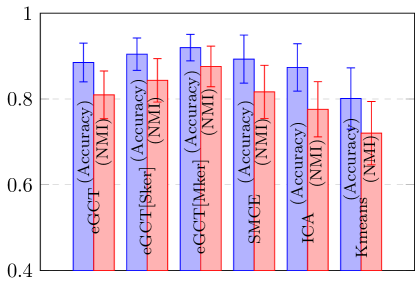
Figure 9: Real fMRI data: State clustering.

8 Conclusions

This paper introduced a novel clustering framework to address all possible clustering tasks in dynamic (brain) networks: state clustering, community detection and subnetwork-state-sequence tracking/identification. Features were extracted by a kernel-based ARMA model, with column spaces of observability matrices mapped to the Grassmann manifold (Grassmannian). A clustering algorithm, the geodesic clustering with tangent spaces, was also provided to exploit the rich underlying Riemannian geometry of the Grassmannian, without the need to know the number of clusters a-priori. The framework was validated on multiple simulated and real datasets and compared against state-of-the-art clustering algorithms. Test results demonstrate that the proposed framework outperforms the competing methods in all clustering tasks. Current research effort includes finding ways to reduce the size of the computational footprint of the framework, and techniques to reject network-wide outlier data.

9 Acknowledgements

The brain network data [50] were provided by the Human Connectome Project, MGH-USC Consortium (Principal Investigators: Bruce R. Rosen, Arthur W. Toga and Van Wedeen; U01MH093765) funded by the NIH Blueprint Initiative for Neuroscience Research grant; the National Institutes of Health grant P41EB015896; and the Instrumentation Grants S10RR023043, 1S10RR023401, 1S10RR019307.

Appendix A Reproducing Kernel Hilbert Spaces

A reproducing kernel Hilbert space $\mathcal{H}$, equipped with inner product $\langle\cdot\mathop{}|\mathop{}\cdot\rangle_{\mathcal{H}}$, is a functional space where each point $g\in\mathcal{H}$ is a function $g:\mathbb{R}^{q}\to\mathbb{R}:\mathbf{y}\mapsto g(\mathbf{y})$, for some $q\in\mathbb{Z}_{>0}$, s.t. the mapping $g\mapsto g(\mathbf{y})$ is continuous, for any choice of $\mathbf{y}$ [56, 37, 57]. There exists a kernel function $\kappa(\cdot,\cdot):\mathbb{R}^{q}\times\mathbb{R}^{q}\to\mathbb{R}$, unique to $\mathcal{H}$, such that (s.t.) $\varphi(\mathbf{y})\coloneqq\kappa(\mathbf{y},\cdot)\in\mathcal{H}$ and $g(\mathbf{y})=\langle g\mathop{}|\mathop{}\varphi(\mathbf{y})\rangle_{\mathcal{H}}$, for any $g\in\mathcal{H}$ and any $\mathbf{y}\in\mathbb{R}^{q}$ [56, 57]. The latter property is the reason for calling kernel $\kappa$ reproducing, and yields the celebrated “kernel trick”: $\kappa(\mathbf{y}_{1},\mathbf{y}_{2})=\langle\kappa(\mathbf{y}_{1},\cdot)\mathop{}|\mathop{}\kappa(\mathbf{y}_{2},\cdot)\rangle_{\mathcal{H}}=\langle\varphi(\mathbf{y}_{1})\mathop{}|\mathop{}\varphi(\mathbf{y}_{2})\rangle_{\mathcal{H}}$, for any $\mathbf{y}_{1},\mathbf{y}_{2}\in\mathbb{R}^{q}$.

Popular examples of reproducing kernels are: 1. The linear $\kappa_{\text{lin}}(\mathbf{y}_{1},\mathbf{y}_{2})\coloneqq\mathbf{y}_{1}^{\intercal}\mathbf{y}_{2}$, where space $\mathcal{H}$ is nothing but $\mathbb{R}^{q}$; 2. the Gaussian $\kappa_{\text{G};\sigma}(\mathbf{y}_{1},\mathbf{y}_{2})\coloneqq\exp[-\lVert\mathbf{y}_{1}-\mathbf{y}_{2}\rVert^{2}/(2\sigma^{2})]$, where $\sigma\in\mathbb{R}_{>0}$ and $\lVert\cdot\rVert$ is the standard Euclidean norm. In this case, $\mathcal{H}$ is infinite dimensional [57]; 3. the Laplacian $\kappa_{\text{L};\sigma}(\mathbf{y}_{1},\mathbf{y}_{2})\coloneqq\exp[-\lVert\mathbf{y}_{1}-\mathbf{y}_{2}\rVert_{1}/\sigma]$, where $\lVert\cdot\rVert_{1}$ stands for the $\ell_{1}$-norm [58]; and 4. the polynomial $\kappa_{\text{poly};r}(\mathbf{y}_{1},\mathbf{y}_{2})\coloneqq(\mathbf{y}_{1}^{\intercal}\mathbf{y}_{2}+1)^{r}$, for some parameter $r\in\mathbb{Z}_{>0}$. There are several ways of generating reproducing kernels via certain operations on well-known kernel functions such as convex combinations, products, etc. [37].

Define $\mathcal{H}^{p}$, for some $p\in\mathbb{Z}_{>0}$, as the space whose points take the following form: $\bm{g}\coloneqq[g_{1},\ldots,g_{p}]^{\intercal}\in\mathcal{H}^{p}$ s.t. $g_{j}\in\mathcal{H}$, $\forall j\in\overline{1,p}$, where $\overline{1,p}$ is a compact notation for $\{1,\ldots,p\}$. For $p^{\prime}\in\mathbb{Z}_{>0}$ and given a matrix $\mathbf{A}\coloneqq[a_{ij}]\in\mathbb{R}^{p^{\prime}\times p}$, the product $\mathbf{A}\bm{g}\in\mathcal{H}^{p^{\prime}}$ stands for the vector-valued function whose $i$th entry is $\sum_{j=1}^{p}a_{ij}g_{j}$. Similarly, define $\mathcal{H}^{p_{1}\times p_{2}}$, for some $p_{1},p_{2}\in\mathbb{Z}_{>0}$, as the space comprising all

$$\bm{\mathcal{G}}\coloneqq\begin{bmatrix}g_{11}&\cdots&g_{1p_{2}}\\ \vdots&\ddots&\vdots\\ g_{p_{1}1}&\cdots&g_{p_{1}p_{2}}\end{bmatrix}\in\mathcal{H}^{p_{1}\times p_{2}}\,,$$

s.t. $g_{ij}\in\mathcal{H}$, $\forall i\in\overline{1,p_{1}}$, $\forall j\in\overline{1,p_{2}}$. Moreover, given $\bm{\mathcal{G}}\in\mathcal{H}^{p_{1}\times p}$ and $\bm{\mathcal{G}}^{\prime}\in\mathcal{H}^{p\times p_{2}}$, define the “product” $\bm{\mathcal{G}}\operatorname{\otimes_{\mathcal{H}}}\bm{\mathcal{G}}^{\prime}$ as the $p_{1}\times p_{2}$ matrix whose $(i,j)$th entry is $[\bm{\mathcal{G}}\operatorname{\otimes_{\mathcal{H}}}\bm{\mathcal{G}}^{\prime}]_{ij}\coloneqq\sum\nolimits_{l=1}^{p}\langle g_{il}\mathop{}|\mathop{}g_{lj}^{\prime}\rangle_{\mathcal{H}}$. In the case where $g_{il}\coloneqq\varphi(\mathbf{y}_{il})=\kappa(\mathbf{y}_{il},\cdot)$ and $g_{lj}^{\prime}\coloneqq\varphi(\mathbf{y}_{lj}^{\prime})=\kappa(\mathbf{y}_{lj}^{\prime},\cdot)$, for some $\mathbf{y}_{il},\mathbf{y}_{lj}^{\prime}$, as in (3), then the kernel trick suggests that the previous formula simplifies to $[\bm{\mathcal{G}}\operatorname{\otimes_{\mathcal{H}}}\bm{\mathcal{G}}^{\prime}]_{ij}=\sum_{l=1}^{p}\kappa(\mathbf{y}_{il},\mathbf{y}_{lj}^{\prime})$.

Appendix B Proof of Proposition 1

By considering a probability space $(\Omega,\Sigma,\operatorname{\mathbb{P}})$, a basis $\{e_{n}\}_{n\in\mathbb{Z}_{>0}}$ of $\mathcal{H}$, and by omitting most of the entailing measure-theoretic details, the expectation of $g=\sum_{n\in\mathbb{Z}_{>0}}\gamma_{n}e_{n}\in\mathcal{H}$, where $\{\gamma_{n}\}_{n\in\mathbb{Z}_{>0}}$ are real-valued RVs, is defined as $\operatorname{\mathbb{E}}(g)\coloneqq\sum_{n\in\mathbb{Z}_{>0}}\operatorname{\mathbb{E}}(\gamma_{n})e_{n}$, provided that the latter sum converges in $\mathcal{H}$. Conditional expectations are similarly defined. All of the expectations appearing in this manuscript are assumed to exist. Due to the linearity of the inner product $\langle\cdot\mathop{}|\mathop{}\cdot\rangle_{\mathcal{H}}$, it can be verified that the conditional expectation $\operatorname{\mathbb{E}}\{\langle g\mathop{}|\mathop{}g^{\prime}\rangle_{\mathcal{H}}{\mathbin{}\mid\mathbin{}}g^{\prime}\}=\operatorname{\mathbb{E}}\{\sum_{n,n^{\prime}}\gamma_{n}\gamma_{n^{\prime}}\langle e_{n}\mathop{}|\mathop{}e_{n^{\prime}}\rangle_{\mathcal{H}}{\mathbin{}\mid\mathbin{}}g^{\prime}\}=\sum_{n^{\prime}}\gamma_{n^{\prime}}\sum_{n}\operatorname{\mathbb{E}}\{\gamma_{n}{\mathbin{}\mid\mathbin{}}g^{\prime}\}\langle e_{n}\mathop{}|\mathop{}e_{n^{\prime}}\rangle_{\mathcal{H}}=\langle\sum_{n}\operatorname{\mathbb{E}}\{\gamma_{n}{\mathbin{}\mid\mathbin{}}g^{\prime}\}e_{n}\mathop{}|\mathop{}\sum_{n^{\prime}}\gamma_{n^{\prime}}e_{n^{\prime}}\rangle_{\mathcal{H}}=\langle\operatorname{\mathbb{E}}\{g{\mathbin{}\mid\mathbin{}}g^{\prime}\}\mathop{}|\mathop{}g^{\prime}\rangle_{\mathcal{H}}$, and $\operatorname{\mathbb{E}}\{\langle g\mathop{}|\mathop{}g^{\prime}\rangle_{\mathcal{H}}\}=\langle\operatorname{\mathbb{E}}(g)\mathop{}|\mathop{}\operatorname{\mathbb{E}}(g^{\prime})\rangle_{\mathcal{H}}$ in the case where $g$ and $g^{\prime}$ are independent. It can be similarly verified that these properties, which hold for the inner product $\langle\cdot\mathop{}|\mathop{}\cdot\rangle$, are inherited by $\operatorname{\otimes_{\mathcal{H}}}$.

Induction on (1) suggests that $\forall\tau\in\mathbb{Z}_{\geq 0}$, $\bm{\varphi}_{t+\tau}=\mathbf{CA}^{\tau}\bm{\psi}_{t}+\sum_{k=1}^{\tau}\mathbf{CA}^{\tau-k}\bm{\omega}_{t+k}+\bm{\upsilon}_{t+\tau}$, where $\sum_{k=1}^{0}\mathbf{CA}^{-k}\bm{\omega}_{t+k}\coloneqq\mathbf{0}$. Then,

$$\bm{f}_{t} \coloneqq\left[\bm{\varphi}_{t}^{\intercal},\bm{\varphi}_{t+1}^{\intercal},\ldots,\bm{\varphi}_{t+m-1}^{\intercal}\right]^{\intercal}$$

$$=\mathbf{O}\bm{\psi}_{t}+\bm{e}_{t}\,,$$ (8)

where

$$\bm{e}_{t}\coloneqq\begin{bmatrix}\bm{\upsilon}_{t}\\ \mathbf{C}\bm{\omega}_{t+1}+\bm{\upsilon}_{t+1}\\ \sum_{k=1}^{2}\mathbf{CA}^{2-k}\bm{\omega}_{t+k}+\bm{\upsilon}_{t+2}\\ \vdots\\ \sum_{k=1}^{m-1}\mathbf{CA}^{m-1-k}\bm{\omega}_{t+k}+\bm{\upsilon}_{t+m-1}\end{bmatrix}\in\mathcal{H}^{mN}\,.$$

By observing that $\bm{\mathcal{F}}_{t}=[\bm{f}_{t},\bm{f}_{t+1},\ldots,\bm{f}_{t+\tau_{\text{f}}-1}]$, it can be verified that $\bm{\mathcal{F}}_{t}=\mathbf{O}\left[\bm{\psi}_{t},\bm{\psi}_{t+1},\ldots,\bm{\psi}_{t+\tau_{\text{f}}-1}\right]+\left[\bm{e}_{t},\bm{e}_{t+1},\ldots,\bm{e}_{t+\tau_{\text{f}}-1}\right]$. Moreover, notice that $\bm{\mathcal{B}}_{t}=[\bm{b}_{t},\bm{b}_{t+1},\ldots,\bm{b}_{t+\tau_{\text{f}}-1}]$, where $\bm{b}_{t}\coloneqq\left[\bm{\varphi}_{t}^{\intercal},\bm{\varphi}_{t-1}^{\intercal},\ldots,\bm{\varphi}_{t-\tau_{\text{b}}+1}^{\intercal}\right]^{\intercal}\in\mathcal{H}^{\tau_{\text{b}}N}$. Hence,

$$\tfrac{1}{\tau_{\text{f}}}\bm{\mathcal{F}}_{t+1}\operatorname{\otimes_{\mathcal{H}}}\bm{\mathcal{B}}_{t}^{\intercal}$$

$${}={} \tfrac{1}{\tau_{\text{f}}}\mathbf{O}\left[\bm{\psi}_{t+1},\ldots,\bm{\psi}_{t+\tau_{\text{f}}}\right]\operatorname{\otimes_{\mathcal{H}}}\bm{\mathcal{B}}_{t}^{\intercal}$$

$$+\tfrac{1}{\tau_{\text{f}}}\left[\bm{e}_{t+1},\ldots,\bm{e}_{t+\tau_{\text{f}}}\right]\operatorname{\otimes_{\mathcal{H}}}\bm{\mathcal{B}}_{t}^{\intercal}$$

$$= \mathbf{O}\,\tfrac{1}{\tau_{\text{f}}}\sum\nolimits_{l=1}^{\tau_{\text{f}}}\bm{\psi}_{t+l}\operatorname{\otimes_{\mathcal{H}}}\bm{b}_{t+l-1}^{\intercal}$$

$$+\tfrac{1}{\tau_{\text{f}}}\sum\nolimits_{l=1}^{\tau_{\text{f}}}\bm{e}_{t+l}\operatorname{\otimes_{\mathcal{H}}}\bm{b}_{t+l-1}^{\intercal}$$

$$= \mathbf{O}\,\tfrac{1}{\tau_{\text{f}}}\sum\nolimits_{l=1}^{\tau_{\text{f}}}\bm{\psi}_{t+l}\operatorname{\otimes_{\mathcal{H}}}[\bm{\psi}_{t+l-1}^{\intercal}\mathbf{C}^{\intercal},\ldots,\bm{\psi}_{t+l-\tau_{\text{b}}}^{\intercal}\mathbf{C}^{\intercal}]$$

$$+\mathbf{O}\,\tfrac{1}{\tau_{\text{f}}}\sum\nolimits_{l=1}^{\tau_{\text{f}}}\bm{\psi}_{t+l}\operatorname{\otimes_{\mathcal{H}}}[\bm{\upsilon}_{t+l-1}^{\intercal},\ldots,\bm{\upsilon}_{t+l-\tau_{\text{b}}}^{\intercal}]$$

$$+\tfrac{1}{\tau_{\text{f}}}\sum\nolimits_{l=1}^{\tau_{\text{f}}}\bm{e}_{t+l}\operatorname{\otimes_{\mathcal{H}}}\bm{b}_{t+l-1}^{\intercal}\,,$$

and (3) is established under the following definitions:

$$\bm{\Pi}_{t+1} {}\coloneqq{} \tfrac{1}{\tau_{\text{f}}}\sum\nolimits_{l=1}^{\tau_{\text{f}}}\bm{\psi}_{t+l}\operatorname{\otimes_{\mathcal{H}}}[\bm{\psi}_{t+l-1}^{\intercal}\mathbf{C}^{\intercal},\ldots,\bm{\psi}_{t+l-\tau_{\text{b}}}^{\intercal}\mathbf{C}^{\intercal}]\,,$$

$$\bm{\mathcal{E}}_{t+1}^{\tau_{\text{f}}} \coloneqq \mathbf{O}\,\tfrac{1}{\tau_{\text{f}}}\sum\nolimits_{l=1}^{\tau_{\text{f}}}\bm{\psi}_{t+l}\operatorname{\otimes_{\mathcal{H}}}[\bm{\upsilon}_{t+l-1}^{\intercal},\ldots,\bm{\upsilon}_{t+l-\tau_{\text{b}}}^{\intercal}]$$

$$+\tfrac{1}{\tau_{\text{f}}}\sum\nolimits_{l=1}^{\tau_{\text{f}}}\bm{e}_{t+l}\operatorname{\otimes_{\mathcal{H}}}\bm{b}_{t+l-1}^{\intercal}\,.$$ (9)

By virtue of the independency between $(\bm{\psi}_{t})_{t}$ and $(\bm{\upsilon}_{t})_{t}$, the zero-mean assumption on $(\bm{\upsilon}_{t})_{t}$, as well as standard properties of the conditional expectation [34, §9.7(k)] with respect to independency, it can be verified that

$$\operatorname{\mathbb{E}}\{\bm{\psi}_{t+l}\operatorname{\otimes_{\mathcal{H}}}[\bm{\upsilon}_{t+l-1}^{\intercal},\ldots,\bm{\upsilon}_{t+l-\tau_{\text{b}}}^{\intercal}]{\mathbin{}\mid\mathbin{}}\bm{\psi}_{t+l}\}$$

$$=\bm{\psi}_{t+l}\operatorname{\otimes_{\mathcal{H}}}[\operatorname{\mathbb{E}}\{\bm{\upsilon}_{t+l-1}^{\intercal}\},\ldots,\operatorname{\mathbb{E}}\{\bm{\upsilon}_{t+l-\tau_{\text{b}}}^{\intercal}\}]=\mathbf{0}\,.$$ (10)

Moreover, for any $i\in\overline{1,m}$ and any $j\in\overline{1,\tau_{\text{b}}}$, the $(i,j)$th $N\times N$ block of the second term in the expression of $\bm{\mathcal{E}}_{t+1}^{\tau_{\text{f}}}$ in (9) becomes equal to

$$\sum\nolimits_{k=1}^{i-1}\mathbf{CA}^{i-1-k}\tfrac{1}{\tau_{\text{f}}}\sum\nolimits_{l=1}^{\tau_{\text{f}}}\bm{\omega}_{t+l+k}\operatorname{\otimes_{\mathcal{H}}}\bm{\varphi}_{t+l-j}^{\intercal}$$

$$\hphantom{=\ }+\tfrac{1}{\tau_{\text{f}}}\sum\nolimits_{l=1}^{\tau_{\text{f}}}\bm{\upsilon}_{t+l+i-1}\operatorname{\otimes_{\mathcal{H}}}\bm{\varphi}_{t+l-j}^{\intercal}$$

$$=\sum\nolimits_{k=1}^{i-1}\mathbf{CA}^{i-1-k}\tfrac{1}{\tau_{\text{f}}}\sum\nolimits_{l=1}^{\tau_{\text{f}}}\bm{\omega}_{t+l+k}\operatorname{\otimes_{\mathcal{H}}}\bm{\psi}_{t+l-j}^{\intercal}\mathbf{C}^{\intercal}$$

$$\hphantom{=\ }+\sum\nolimits_{k=1}^{i-1}\mathbf{CA}^{i-1-k}\tfrac{1}{\tau_{\text{f}}}\sum\nolimits_{l=1}^{\tau_{\text{f}}}\bm{\omega}_{t+l+k}\operatorname{\otimes_{\mathcal{H}}}\bm{\upsilon}_{t+l-j}^{\intercal}$$

$$\hphantom{=\ }+\tfrac{1}{\tau_{\text{f}}}\sum\nolimits_{l=1}^{\tau_{\text{f}}}\bm{\upsilon}_{t+l+i-1}\operatorname{\otimes_{\mathcal{H}}}\bm{\psi}_{t+l-j}^{\intercal}\mathbf{C}^{\intercal}$$

$$\hphantom{=\ }+\tfrac{1}{\tau_{\text{f}}}\sum\nolimits_{l=1}^{\tau_{\text{f}}}\bm{\upsilon}_{t+l+i-1}\operatorname{\otimes_{\mathcal{H}}}\bm{\upsilon}_{t+l-j}^{\intercal}\,.$$ (11)

Since $t+l+k>t+l>t+l-j$ and $t+l+i-1\geq t+l>t+l-j$, $\bm{\psi}_{t+l-j}$ precedes $\bm{\omega}_{t+l+k}$ on the time axis, while $\bm{\upsilon}_{t+l+i-1}$ precedes $\bm{\upsilon}_{t+l-j}$. Hence, due to independency, $\operatorname{\mathbb{E}}\{\bm{\omega}_{t+l+k}\operatorname{\otimes_{\mathcal{H}}}\bm{\psi}_{t+l-j}^{\intercal}{\mathbin{}\mid\mathbin{}}\bm{\psi}_{t^{\prime}}\}=\operatorname{\mathbb{E}}\{\bm{\omega}_{t+l+k}{\mathbin{}\mid\mathbin{}}\bm{\psi}_{t^{\prime}}\}\operatorname{\otimes_{\mathcal{H}}}\bm{\psi}_{t+l-j}^{\intercal}=\operatorname{\mathbb{E}}\{\bm{\omega}_{t+l+k}\}\operatorname{\otimes_{\mathcal{H}}}\bm{\psi}_{t+l-j}^{\intercal}=\mathbf{0}$, and $\operatorname{\mathbb{E}}\{\bm{\upsilon}_{t+l+i-1}\operatorname{\otimes_{\mathcal{H}}}\bm{\upsilon}_{t+l-j}^{\intercal}{\mathbin{}\mid\mathbin{}}\bm{\psi}_{t^{\prime}}\}=\operatorname{\mathbb{E}}\{\bm{\upsilon}_{t+l+i-1}\}\operatorname{\otimes_{\mathcal{H}}}\operatorname{\mathbb{E}}\{\bm{\upsilon}_{t+l-j}^{\intercal}\}=\mathbf{0}$. It can be also similarly verified that $\operatorname{\mathbb{E}}\{\bm{\omega}_{t+l+k}\operatorname{\otimes_{\mathcal{H}}}\bm{\upsilon}_{t+l-j}^{\intercal}{\mathbin{}\mid\mathbin{}}\bm{\psi}_{t^{\prime}}\}=\mathbf{0}$ and $\operatorname{\mathbb{E}}\{\bm{\upsilon}_{t+l+i-1}\operatorname{\otimes_{\mathcal{H}}}\bm{\psi}_{t+l-j}^{\intercal}{\mathbin{}\mid\mathbin{}}\bm{\psi}_{t^{\prime}}\}=\mathbf{0}$. As a result, the conditional expectation of (11), given $\bm{\psi}_{t^{\prime}}$, becomes $\mathbf{0}$. This observation and (10) establish claim (4) of the proposition.

Under the assumptions on wide-sense stationarity, the covariance sequences of the processes $(\bm{\omega}_{t}\operatorname{\otimes_{\mathcal{H}}}\bm{\psi}_{t-\tau}^{\intercal})_{t}$, $(\bm{\omega}_{t}\operatorname{\otimes_{\mathcal{H}}}\bm{\upsilon}_{t-\tau}^{\intercal})_{t}$, $(\bm{\upsilon}_{t}\operatorname{\otimes_{\mathcal{H}}}\bm{\psi}_{t-\tau}^{\intercal})_{t}$, $(\bm{\psi}_{t}\operatorname{\otimes_{\mathcal{H}}}\bm{\upsilon}_{t-\tau}^{\intercal})_{t}$, $(\bm{\upsilon}_{t}\operatorname{\otimes_{\mathcal{H}}}\bm{\upsilon}_{t-\tau}^{\intercal})_{t}$, $\forall\tau\in\mathbb{Z}_{>0}$, are summable over all lags; in fact, the covariances of non-zero lags become zero due to the assumptions on independency. Hence, by the mean-square ergodic theorem [59], sample averages of the previous processes converge in the mean-square ($\mathcal{L}_{2}$-) sense to their ensemble means. For example, applying $\lim_{\tau_{\text{f}}\to\infty}$, in the mean-square sense, to the first part of $\bm{\mathcal{E}}_{t+1}^{\tau_{\text{f}}}$ in (9) and by recalling standard properties of the conditional expectation [34, §9.7(a)] yield

$$\mathbf{O}\lim_{\tau_{\text{f}}\to\infty}\tfrac{1}{\tau_{\text{f}}}\sum\nolimits_{l=1}^{\tau_{\text{f}}}\bm{\psi}_{t+l}\operatorname{\otimes_{\mathcal{H}}}[\bm{\upsilon}_{t+l-1}^{\intercal},\ldots,\bm{\upsilon}_{t+l-\tau_{\text{b}}}^{\intercal}]$$

$$=\mathbf{O}\operatorname{\mathbb{E}}\{\bm{\psi}_{t+l}\operatorname{\otimes_{\mathcal{H}}}[\bm{\upsilon}_{t+l-1}^{\intercal},\ldots,\bm{\upsilon}_{t+l-\tau_{\text{b}}}^{\intercal}]\}$$

$$=\mathbf{O}\operatorname{\mathbb{E}}\{\operatorname{\mathbb{E}}\{\bm{\psi}_{t+l}\operatorname{\otimes_{\mathcal{H}}}[\bm{\upsilon}_{t+l-1}^{\intercal},\ldots,\bm{\upsilon}_{t+l-\tau_{\text{b}}}^{\intercal}]{\mathbin{}\mid\mathbin{}}\bm{\psi}_{t+l}\}\}=\mathbf{0}\,.$$ (12)

By following similar arguments, it can be verified that the application of $\lim_{\tau_{\text{f}}\to\infty}$ to (11) renders the second part of (9) equal to $\mathbf{0}$. This finding and (12) establish the final claim of the proposition.

References

- Fan et al. [2018] H. Fan, L. Zheng, C. Yan, Y. Yang, Unsupervised person re-identification: Clustering and fine-tuning, ACM Transactions on Multimedia Computing, Communications, and Applications (TOMM) 14 (2018) 83.
- Abuarqoub et al. [2017] A. Abuarqoub, M. Hammoudeh, B. Adebisi, S. Jabbar, A. Bounceur, H. Al-Bashar, Dynamic clustering and management of mobile wireless sensor networks, Computer Networks 117 (2017) 62–75.
- Huang and Chen [2016] S.-Y. Huang, H. Chen, Exploring the online underground marketplaces through topic-based social network and clustering, in: 2016 IEEE Conference on Intelligence and Security Informatics (ISI), IEEE, 2016, pp. 145–150.
- Märtens et al. [2017] M. Märtens, J. Meier, A. Hillebrand, P. Tewarie, P. Van Mieghem, Brain network clustering with information flow motifs, Applied Network Science 2 (2017) 25.
- Feldt et al. [2011] S. Feldt, P. Bonifazi, R. Cossart, Dissecting functional connectivity of neuronal microcircuits: Experimental and theoretical insights, Trends in Neurosciences 34 (2011) 225–236.
- Pedersen et al. [2015] M. Pedersen, A. H. Omidvarnia, J. M. Walz, G. D. Jackson, Increased segregation of brain networks in focal epilepsy: An fMRI graph theory finding, NeuroImage: Clinical 8 (2015) 536–542.
- Broyd et al. [2009] S. J. Broyd, C. Demanuele, S. Debener, S. K. Helps, C. J. James, E. J. Sonuga-Barke, Default-mode brain dysfunction in mental disorders: A systematic review, Neuroscience & Biobehavioral Reviews 33 (2009) 279–296.
- Stam et al. [2009] C. J. Stam, W. De Haan, A. Daffertshofer, B. F. Jones, I. Manshanden, A. M. Van Cappellen Van Walsum, T. Montez, J. P. A. Verbunt, J. C. De Munck, B. W. Van Dijk, H. W. Berendse, P. Scheltens, Graph theoretical analysis of magnetoencephalographic functional connectivity in Alzheimer’s disease, Brain 132 (2009) 213–224.
- Anderson et al. [2014] M. Anderson, G.-S. Fu, R. Phlypo, T. Adalı, Independent vector analysis: Identification conditions and performance bounds, IEEE Transactions on Signal Processing 62 (2014) 4399–4410.
- Ma et al. [2014] S. Ma, V. D. Calhoun, R. Phlypo, T. Adali, Dynamic changes of spatial functional network connectivity in healthy individuals and schizophrenia patients using independent vector analysis, Neuroimage 90 (2014) 196–206.
- Ou et al. [2015] J. Ou, L. Xie, C. Jin, X. Li, D. Zhu, R. Jiang, Y. Chen, J. Zhang, L. Li, T. Liu, Characterizing and differentiating brain state dynamics via hidden Markov models, Brain Topography 28 (2015) 666–679.
- Zheng et al. [2017] Y. Zheng, B. Jeon, L. Sun, J. Zhang, H. Zhang, Student’s t-hidden Markov model for unsupervised learning using localized feature selection, IEEE Transactions on Circuits and Systems for Video Technology 28 (2017) 2586–2598.
- Masuda and Holme [2019] N. Masuda, P. Holme, Detecting sequences of system states in temporal networks, Scientific Reports 9 (2019) 795.
- Lu et al. [2015] H. Lu, M. Halappanavar, A. Kalyanaraman, Parallel heuristics for scalable community detection, Parallel Computing 47 (2015) 19–37.
- Xiang et al. [2016] J. Xiang, T. Hu, Y. Zhang, K. Hu, J.-M. Li, X.-K. Xu, C.-C. Liu, S. Chen, Local modularity for community detection in complex networks, Physica A: Statistical Mechanics and its Applications 443 (2016) 451–459.
- Orhan et al. [2012] U. Orhan, M. Hekim, M. Ozer, Epileptic seizure detection using probability distribution based on equal frequency discretization, J. Medical Systems 36 (2012) 2219–2224.
- Li et al. [2017] P. Li, H. Dau, G. Puleo, O. Milenkovic, Motif clustering and overlapping clustering for social network analysis, in: IEEE INFOCOM 2017-IEEE Conference on Computer Communications, IEEE, 2017, pp. 1–9.
- Mammone et al. [2011] N. Mammone, G. Inuso, F. La Foresta, M. Versaci, F. C. Morabito, Clustering of entropy topography in epileptic electroencephalography, Neural Computing and Applications 20 (2011) 825–833.
- Mateos et al. [2019] G. Mateos, S. Segarra, A. G. Marques, A. Ribeiro, Connecting the dots: Identifying network structure via graph signal processing, IEEE Signal Processing Magazine 36 (2019) 16–43.
- Segarra et al. [2017] S. Segarra, A. G. Marques, G. Mateos, A. Ribeiro, Network topology inference from spectral templates, IEEE Transactions on Signal and Information Processing over Networks 3 (2017) 467–483.
- Al-Sharoa et al. [2018] E. Al-Sharoa, M. Al-Khassaweneh, S. Aviyente, Tensor based temporal and multi-layer community detection for studying brain dynamics during resting state fMRI, IEEE Trans. Biomedical Engineering (2018). doi:10.1109/TBME.2018.2854676.
- Bréchet et al. [2019] L. Bréchet, D. Brunet, G. Birot, R. Gruetter, C. M. Michel, J. Jorge, Capturing the spatiotemporal dynamics of self-generated, task-initiated thoughts with EEG and fMRI, NeuroImage 194 (2019) 82–92.
- Lim et al. [2018] S. H. Lim, H. Nisar, K. W. Thee, V. V. Yap, A novel method for tracking and analysis of EEG activation across brain lobes, Biomedical Signal Processing and Control 40 (2018) 488–504.
- Slavakis et al. [2018] K. Slavakis, S. Salsabilian, D. S. Wack, S. F. Muldoon, H. E. Baidoo-Williams, J. M. Vettel, M. Cieslak, S. T. Grafton, Clustering brain-network time series by Riemannian geometry, IEEE Trans. Signal and Information Processing over Networks 4 (2018) 519–533.
- Mateos et al. [2019] G. Mateos, S. Segarra, A. G. Marques, A. Ribeiro, Connecting the dots: Identifying network structure via graph signal processing, IEEE Signal Processing Magazine 36 (2019) 16–43.
- Wang et al. [2015] X. Wang, K. Slavakis, G. Lerman, Multi-manifold modeling in non-euclidean spaces, in: Artificial Intelligence and Statistics, 2015, pp. 1023–1032.
- Wang et al. [2014] X. Wang, K. Slavakis, G. Lerman, Riemannian multi-manifold modeling, arXiv:1410.0095 (2014).
- Yger et al. [2017] F. Yger, M. Berar, F. Lotte, Riemannian approaches in brain-computer interfaces: A review, IEEE Transactions on Neural Systems and Rehabilitation Engineering 25 (2017) 1753–1762.
- Ogawa et al. [1990] S. Ogawa, T.-M. Lee, A. R. Kay, D. W. Tank, Brain magnetic resonance imaging with contrast dependent on blood oxygenation, Proc. National Academy of Sciences 87 (1990) 9868–9872.
- Drezet [1998] P. M. L. Drezet, Support vector machines for system identification, in: UKACC International Conference on Control, 1998, pp. 688–692.
- Martínez-Ramón et al. [2006] M. Martínez-Ramón, J. L. Rojo-Alvarez, G. Camps-Valls, J. Muñoz-Marí, E. Soria-Olivas, A. R. Figueiras-Vidal, Support vector machines for nonlinear kernel ARMA system identification, IEEE Transactions on Neural Networks 17 (2006) 1617–1622.
- Shpigelman et al. [2009] L. Shpigelman, H. Lalazar, E. Vaadia, Kernel-ARMA for hand tracking and brain-machine interfacing during 3D motor control, in: D. Koller, D. Schuurmans, Y. Bengio, L. Bottou (Eds.), Advances in Neural Information Processing Systems 21, Curran Associates, Inc., 2009, pp. 1489–1496.
- Pincombe [2005] B. Pincombe, Anomaly detection in time series of graphs using ARMA processes, ASOR Bull. 24 (2005) 1–10.
- Williams [1991] D. Williams, Probability with Martingales, Cambridge University Press, 1991.
- Ben-Israel and Greville [2003] A. Ben-Israel, T. N. Greville, Generalized Inverses: Theory and Applications, volume 15, Springer Science & Business Media, 2003.
- Tu [2008] L. W. Tu, An Introduction to Manifolds, Springer, 2008.
- Scholkopf and Smola [2001] B. Scholkopf, A. J. Smola, Learning with Kernels, MIT Press, 2001.
- Yang et al. [2011] W. Yang, C. Sun, L. Zhang, A multi-manifold discriminant analysis method for image feature extraction, Pattern Recognition 44 (2011) 1649–1657.
- Elhamifar and Vidal [2011] E. Elhamifar, R. Vidal, Sparse manifold clustering and embedding, in: Advances in Neural Information Processing Systems, 2011, pp. 55–63.
- Aynaud and Guillaume [2010] T. Aynaud, J.-L. Guillaume, Static community detection algorithms for evolving networks, in: Proc. IEEE WiOpt, 2010, pp. 513–519.
- Absil et al. [2004] P.-A. Absil, R. Mahony, R. Sepulchre, Riemannian geometry of Grassmann manifolds with a view on algorithmic computation, Acta Applicandae Mathematicae 80 (2004) 199–220.
- De Meo et al. [2011] P. De Meo, E. Ferrara, G. Fiumara, A. Provetti, Generalized Louvain method for community detection in large networks, in: Proc. IEEE International Conference on Intelligent Systems Design and Applications, 2011, pp. 88–93.
- Vijay and Selvakumar [2015] K. Vijay, K. Selvakumar, Brain fMRI clustering using interaction K-means algorithm with PCA, in: Proc. IEEE ICCSP, 2015, pp. 909–913.
- Allen et al. [2014] E. A. Allen, E. Damaraju, S. M. Plis, E. B. Erhardt, T. Eichele, V. D. Calhoun, Tracking whole-brain connectivity dynamics in the resting state, Cerebral Cortex 24 (2014) 663–676.
- Sockeel et al. [2016] S. Sockeel, D. Schwartz, M. Pélégrini-Issac, H. Benali, Large-scale functional networks identified from resting-state EEG using spatial ICA, PloS one 11 (2016) e0146845.
- Barnett and Seth [2014] L. Barnett, A. K. Seth, The MVGC multivariate Granger causality toolbox: A new approach to Granger-causal inference, Journal of neuroscience methods 223 (2014) 50–68.
- Duggento et al. [2018] A. Duggento, L. Passamonti, G. Valenza, R. Barbieri, M. Guerrisi, N. Toschi, Multivariate Granger causality unveils directed parietal to prefrontal cortex connectivity during task-free MRI, Scientific reports 8 (2018) 5571.
- Al-Sharoa et al. [2017] E. Al-Sharoa, M. Al-Khassaweneh, S. Aviyente, A tensor based framework for community detection in dynamic networks, in: Proc. IEEE ICASSP, 2017, pp. 2312–2316.
- Schütze et al. [2008] H. Schütze, C. D. Manning, P. Raghavan, Introduction to Information Retrieval, volume 39, Cambridge University Press, 2008.
- Glasser et al. [2013] M. F. Glasser, S. N. Sotiropoulos, J. A. Wilson, T. S. Coalson, B. Fischl, J. L. Andersson, J. Xu, S. Jbabdi, M. Webster, J. R. Polimeni, et al., The minimal preprocessing pipelines for the human connectome project, Neuroimage 80 (2013) 105–124.
- Jenkinson et al. [2002] M. Jenkinson, P. Bannister, M. Brady, S. Smith, Improved optimization for the robust and accurate linear registration and motion correction of brain images, Neuroimage 17 (2002) 825–841.
- Tzourio-Mazoyer et al. [2002] N. Tzourio-Mazoyer, B. Landeau, D. Papathanassiou, F. Crivello, O. Etard, N. Delcroix, B. Mazoyer, M. Joliot, Automated anatomical labeling of activations in SPM using a macroscopic anatomical parcellation of the MNI MRI single-subject brain, Neuroimage 15 (2002) 273–289.
- Schaefer et al. [2017] A. Schaefer, R. Kong, E. M. Gordon, T. O. Laumann, X.-N. Zuo, A. J. Holmes, S. B. Eickhoff, B. T. Yeo, Local-global parcellation of the human cerebral cortex from intrinsic functional connectivity mri, Cerebral Cortex 28 (2017) 3095–3114.
- Huang et al. [2005] Y.-Z. Huang, M. J. Edwards, E. Rounis, K. P. Bhatia, J. C. Rothwell, Theta burst stimulation of the human motor cortex, Neuron 45 (2005) 201–206.
- Medaglia et al. [2018] J. D. Medaglia, W. Huang, E. A. Karuza, A. Kelkar, S. L. Thompson-Schill, A. Ribeiro, D. S. Bassett, Functional alignment with anatomical networks is associated with cognitive flexibility, Nature Human Behaviour 2 (2018) 156.
- Aronszajn [1950] N. Aronszajn, Theory of reproducing kernels, Trans. American Mathematical Society 68 (1950) 337–404.
- Slavakis et al. [2014] K. Slavakis, P. Bouboulis, S. Theodoridis, Online learning in reproducing kernel Hilbert spaces, in: Academic Press Library in Signal Processing: Signal Processing Theory and Machine Learning, volume 1, 2014, pp. 883–987.
- Sriperumbudur et al. [2010] B. K. Sriperumbudur, A. Gretton, K. Fukumizu, B. Schölkopf, G. R. G. Lanckriet, Hilbert space embeddings and metrics on probability measures, J. Machine Learning Research 11 (2010) 1517–1561.
- Petersen [1983] K. Petersen, Ergodic Theory, Cambridge University Press, 1983.