Superfluid turbulence driven by cylindrically symmetric thermal counterflow

Abstract

We show by direct numerical simulations that the turbulence generated by steadily heating a long cylinder immersed in helium II is strongly inhomogeneous and consists of a dense turbulent layer of quantized vortices localized around the cylinder. We analyse the properties of this superfluid turbulence in terms of radial distribution of the vortex line density and the anisotropy and we compare these properties to the better known properties of homogeneous counterflow turbulence in channels.

I Introduction

Since the early experiments of Vinen Vinen , superfluid turbulence has been typically studied in a long channel which is closed at one end and connected to the helium bath at the other end. At the closed end, an electrical resistor steadily dissipates a known heat flux which drives helium’s two components in opposite directions: the normal fluid towards the bath and the superfluid towards the resistor; this motion is called thermal counterflow. If the applied heat flux exceeds a critical value, an extra thermal resistance is observed, caused by the appearance of a turbulent tangle of quantised vortex lines which limit the heat-conducting properties of liquid helium. Following Vinen’s work, thermal counterflow has been the subject of many experiments and numerical simulations which have revealed the nature and the dynamics of turbulent vortex lines. Recently-investigated aspects of the problem include the Lagrangian velocity statistics of tracer particles which are used to visualize the turbulence Svancara2018 ; Mastracci2019 , the coupled dynamics of normal fluid and vortex lines Yui2018 , the comparison with ordinary turbulence Biferale2019 , and the effects induced by the channel’s walls BaggaleyLaurie2015 . In the last case the density of vortex lines is not spatially uniform; indeed inhomogeneous superfluid turbulence is still poorly understood.

This work is concerned with perhaps the simplest configuration of inhomogeneous superfluid turbulence: steady radial counterflow around a long heated cylinder. This flow is simple to set-up in the laboratory, requiring only a thin metal wire across a cell containing liquid helium through which an electrical current dissipates a known heat flux into the surrounding liquid. The natural question which we address is whether the superfluid turbulence around the heated cylinder differs from the standard case studied by Vinen. In particular we want to find whether, and under what conditions, the local vortex line density achieves any statistically steady state, and determine its radial distribution. Besides turbulence, the problem of the heated cylinder has motivations of engineering heat transfer and applications such as hot-wire anemometry Duri2015 in liquid helium note0 .

II Formulation of the problem and numerical method

We numerically model the thermal counterflow generated by a heated, infinitely long, cylinder of radius $a$ immersed in liquid helium II. We assume that the cylinder generates a constant heat flux, $q$, which determines the radial normal velocity ${\mbox{$v_{0}$}}={\mbox{$v_{n}$}}(a)$ at the cylinder’s surface $r=a$ (hereafter $r$ is the radial coordinate).

We assume that the temperature of helium is uniform throughout the whole flow domain, $r>a$, so that the normal and superfluid densities and all other thermodynamic quantities are constant. First we consider the normal (${\bf{v}}_{n}$) and superfluid (${\bf{V}}_{s}$) velocity distributions in the case where there is no superfluid turbulence. In the thermal counterflow generated by the heated surface of the cylinder, the normal fluid moves radially out with positive radial velocity ${\mbox{$v_{n}$}}=a{\mbox{$v_{0}$}}/r$ taking heat away (hereafter the subscript $r$ in the radial components of ${\bf{v}}_{n}$ and ${\bf{V}}_{s}$ is omitted). In the steady-state flow regime, the counterflow condition

$${\mbox{$\rho_{n}$}}{\bf{v}}_{n}+{\mbox{$\rho_{s}$}}{\bf{V}}_{s}={\bf 0}\,,$$ (1)

(where $\rho_{n}$ and $\rho_{s}$ are respectively the normal and superfluid densities) yields the following radial superfluid velocity:

$${\mbox{$V_{s}$}}=-{\mbox{$\rho_{n}$}}a{\mbox{$v_{0}$}}/({\mbox{$\rho_{s}$}}r),$$ (2)

where the minus sign means that ${\bf{V}}_{s}$ points radially inwards.

Hereafter we consider the case in which helium II becomes turbulent. For the sake of simplicity, we assume that the driving velocity $v_{0}$ is large enough that superfluid vortex lines are generated, but not so large that the normal fluid becomes turbulent. In other words, we assume the so-called T1 regime Tough of counterflow turbulence. We treat the superfluid velocity, ${\bf{V}}_{s}$, which enforces the counterflow condition (1) and therefore is radially distributed according to Eq. (2), as the externally applied superflow; in this way, in the presence of the turbulent vortex tangle, the total superfluid velocity ${\bf{v}}_{s}$ can be decomposed as ${\bf{v}}_{s}={\bf{v}}_{s}^{i}+{\bf{V}}_{s}$, where ${\bf{v}}_{s}^{i}$ is the self-induced velocity generated by the vortex tangle. In the framework of the vortex filament method, we model quantum vortex filaments as infinitesimally thin space curves $\bf{s}(\xi,\,t)$ which move according to the Schwarz equation Schwarz1988

$$\frac{{\rm d}\bf{s}}{{\rm d}t}={\bf{v}}_{s}+\alpha\bf{s}^{\prime}\times({\bf{v}}_{n}-{\bf{v}}_{s})-\alpha^{\prime}\bf{s}^{\prime}\times[\bf{s}^{\prime}\times({\bf{v}}_{n}-{\bf{v}}_{s})],$$ (3)

where $t$ is time, $\alpha$ and $\alpha^{\prime}$ are dimensionless temperature-dependent friction coefficients Donnelly-Barenghi , $\bf{s}^{\prime}=\rm{d}\bf{s}/\rm{d}\xi$ is the unit tangent vector at the point $\bf{s}$, and $\xi$ is the arc length.

At the point $\bf{s}$, the self-induced velocity is given by the Biot-Savart law Adachi ; BagBar2012

$${\bf{v}}_{s}^{i}=-\frac{\kappa}{4\pi}\oint_{\cal L}\frac{(\bf{s}-\bf{r})}{|\bf{s}-\bf{r}|^{3}}\times\rm{d}\bf{r},$$ (4)

where $\kappa=9.97\times 10^{-4}\,{\rm cm^{2}/s}$ is the quantum of circulation, and the line integral extends over the entire vortex configuration $\cal L$.

We numerically simulate the emergence and evolution of the vortex tangle for a cylinder of given radius $a$ and normal fluid velocity $v_{0}$ at the cylinder’s surface. In all simulations reported here we assume the values $a=0.1~{}\rm cm$ and ${\mbox{$v_{0}$}}=0.6~{}\rm cm/s$. We also assume that, in the bulk, the temperature of the liquid helium is $T=1.3~{}\rm K$. At this temperature, the normal fluid and superfluid densities are ${\mbox{$\rho_{n}$}}=6.522\times 10^{-3}\,{\rm g/cm^{3}}$ and ${\mbox{$\rho_{s}$}}=0.1386\,{\rm g/cm^{3}}$ respectively, and the mutual friction coefficients are $\alpha=0.034$ and $\alpha^{\prime}=1.383\times 10^{-2}$.

Our calculation is performed in a domain open in the direction orthogonal to the cylinder and periodic in the coordinate $z$ along the axis of cylinder, with a period of $0.2~{}\rm cm$. The vortex lines are discretized by Lagrangian points $\bf{s}_{j}$ for $j=1,\dots,N$ held at minimum separation $\Delta\xi=2\times 10^{-3}$ cm; the Schwarz equation (3) is time-stepped using a fourth-order Adams-Bashforth method with typical time step $\Delta t=5\times 10^{-5}$ s. The de-singularization of the Biot-Savart integrals and the technique to numerically perform vortex reconnections when vortex lines approach each other sufficiently close are all described in Refs. BagBar2012 ; Baggaley2012 ; Laurie-Baggaley2015 . The number of Lagrangian points changes with time and becomes very large (typically of the order of $N\approx 10^{5}$) in the final statistically steady-state regime of turbulence. To reduce the computation time, during the initial transient from time $t=0$ to the time $t_{s}$ when the tangle is still dilute and the vortex length builds up, the Biot-Savart integral is approximated by the Local Induction Approximation (LIA) Schwarz1978 . At the somewhat arbitrary moment $t_{s}$, when the tangle becomes dense in the region adjacent to the cylinder’s surface note1 , we switch from the LIA to the full Biot-Savart integral in the tree-algorithm approximation (the switching criterion will be described in section IV). The tree-algorithm (described and tested in Ref. BagBar2012 ), is clearly suitable for random tangles such as ours, where contributions to the velocity field at a point arising from far-away vortex lines are less important than contributions arising from vortex lines in the immediate neighbourhood of that point.

The initial transient under LIA does not affect our final results for the following reason. The characteristic time scale for the Biot-Savart interaction between the vortex lines is of the order of the eddy turnover time $\tau\approx\ell/u_{\ell}\approx\ell^{2}/\kappa$ where $\ell$ is the distance between vortices in a given region. Taking typical values $L\approx 1000$ to $6000~{}\rm cm^{-2}$ for the vortex line density in the saturated regime at distances $a<r<5a$, we find $\tau\approx 0.2$ to $1~{}\rm s$, which is much shorter than the time-scale $\approx 23~{}\rm s$ of the evolution computed under the Biot-Savart law.

The boundary conditions at the cylinder’s surface are implemented using the method of images, which enforces the condition by ensuring that the boundary is a streamline. An image of the vortex line configuration is generated with

$$\mathbf{s}_{\text{image}}=\left(\frac{a^{2}s_{x}}{s_{x}^{2}+s_{y}^{2}},\,\frac{a^{2}s_{y}}{s_{x}^{2}+s_{y}^{2}},\,s_{z}\right),$$ (5)

where $(s_{x},s_{y},s_{z})$ are the $(x,y,z)$ components of the Lagrangian discretization point $\mathbf{s}$ of the original vortex line. Similarly to the reconnection procedure used in the bulk of the fluid when two vortex lines collide, vortex lines that pass within a distance of the order of the minimum separation from the surface of the cylinder are reconnected algorithmically to their images.

The initial state consists of vortex rings placed in the immediate vicinity of the cylinder’s surface, whose orientations are chosen such that the initial velocity of each ring is in the outward radial direction, see Figure 1. The initial radii of the rings are drawn from a normal distribution with mean $0.007~{}\rm~{}cm$ and standard deviation $0.001~{}\rm cm$. We have also experimented with simpler initial vortex configurations, such as randomly oriented vortex rings, finding that they tend to require a longer transient to achieve a statistically identical turbulent steady-state.

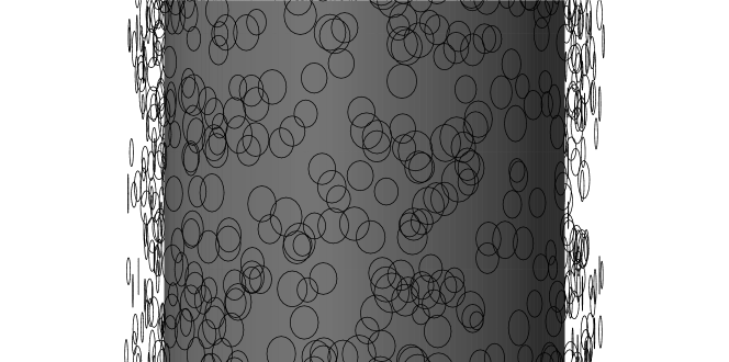
Figure 1: Typical initial vortex configuration of vortex rings in the vicinity of the cylinder.

III Absence of steady-state for uniform temperature

First we consider the case in which the temperature is uniform throughout the whole flow domain $r>a$ with value $T=1.3~{}\rm K$. As it can be seen from Figure 2, which illustrates the time evolution of the total vortex line length $\Lambda$ within the whole flow domain, the vortex tangle does not saturate to a statistically steady state. We find that at first $\Lambda$ increases, and then crashes to zero, independently of the initial condition used. This result (the absence of a steady-state), which we obtain both under an initial LIA evolution, as described in the previous section, and also under the Biot-Savart law from start to finish, is consistent with recent calculations by Varga Varga2019 who simulated spherically symmetric counterflow using the same vortex filament method. In a recent paper Sergeev-EPL , we have explained the absence of a steady-state solution using the Hall-Vinen-Bekarevich-Khalatnikov (HVBK) equations Khalatnikov-book , i.e. a continuous model of the laminar vortex flow as well as the turbulent flow Roche2009 of helium II. According to the HVBK equations, if the temperature is uniform and the helium’s properties are constant in the flow domain, then there exists only one steady-state solution corresponding to a particular choice of $v_{0}$, that is, a single value of heat flux. For an arbitrary heat flux, there is no steady-state solution.

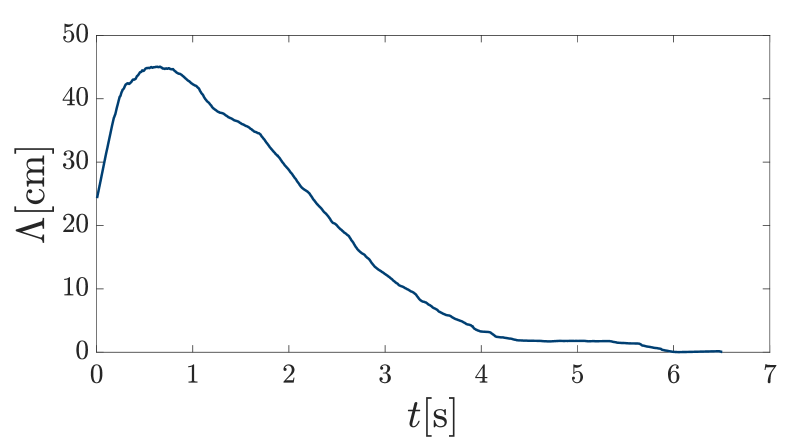
Figure 2: The total vortex line length $\Lambda$ vs time in the case where the temperature and mutual friction coefficients are uniform throughout the entire flow domain. Notice that the turbulence decays.

IV Turbulent steady-state for nonuniform friction

According to Ref. Sergeev-EPL , the HVBK equations allow steady-state solutions only in the case where the temperature in the bulk of helium is no longer assumed constant, but is found as a function of radial coordinate from the equations; this means that the normal fluid and superfluid densities as well as all other thermodynamic variables and the mutual friction coefficients depend on the radial coordinate. Unfortunately it would be computationally and conceptually difficult to include this spatial variability in the vortex filament method (for example, Eq. (4) assumes that the superfluid is incompressible). At the same time, in order to make progress in this problem, it would be useful to go beyond the HVBK equations and their limitations when applied to turbulence (if the vortex lines are randomly oriented, the superfluid vorticity is not related to the vortex line density BaggaleyLaurie2012 in the simple way assumed by the HVBK equations).

Based on these motivations and our previous findings Sergeev-EPL here we develop a minimal numerical model of turbulent radial counterflow which captures the essential physics of the problem and lets us use the vortex filament model (the best model available for turbulent helium II at nonzero temperatures): we assume that the normal fluid and superfluid densities are constant throughout the whole flow domain, but the mutual friction coefficients vary with the radial coordinate, that is $\alpha=\alpha(r)$ and $\alpha^{\prime}=\alpha^{\prime}(r)$. Furthermore, we assume that the behavior of $\alpha$ and $\alpha^{\prime}$ mimics the radial profiles of these coefficients that follow from a typical radial distribution of temperature described in Ref. Sergeev-EPL . The radial distributions of $\alpha$ and $\alpha^{\prime}$ used in our numerical simulations are shown in the top panel of Figure 3.

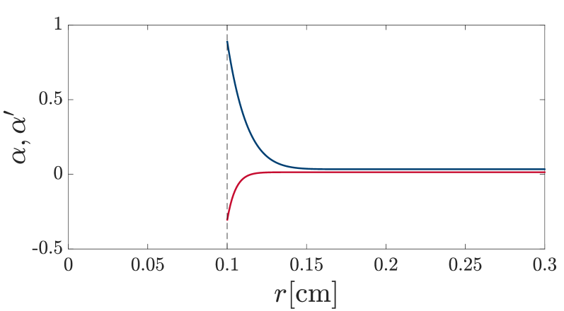
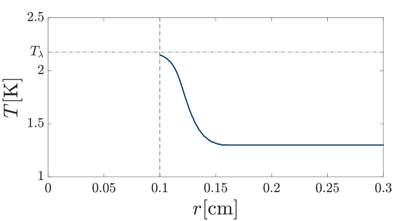
Figure 3: Top panel: mutual friction coefficients $\alpha$ (top, blue) and $\alpha^{\prime}$ (bottom,red) as functions of the radial coordinate. Bottom panel: radial profile of temperature corresponding to the distributions of mutual friction coefficients shown in the top panel.

These distributions conform to $\alpha(r)$ and $\alpha^{\prime}(r)$ corresponding to the case where the surface temperature is ${\mbox{$T_{0}$}}=2.15$ K, and the bulk temperature of helium is $1.3\rm~{}K$. Note that the mutual friction coefficients undergo a rapid change only within a relatively narrow region (about half a radius $a$ from the cylinder’s surface) before saturating to constant values in the bulk of helium. The radial profile of temperature corresponding to the distributions of $\alpha$ and $\alpha^{\prime}$ shown in the top panel of Figure 3 is illustrated in the bottom panel of this figure.

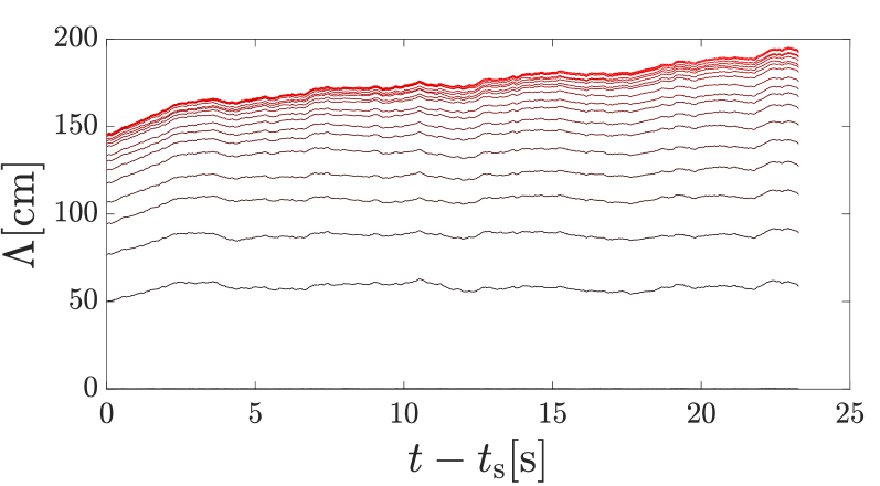
Figure 4: Evolution of the total line length, $\Lambda_{n}$ vs time (starting from the time $t_{s}$ defined in the text) within cylindrical shells, of outer radii increasing with $n$, adjacent to the cylinder’s surface, see text for details. The curves, from bottom to top, correspond to $n=1,\,2,\,3,\,\dots$.

Under the assumptions of our minimal model, the saturation of the tangle to a statistically steady-state is illustrated by Figure 4 which shows the total vortex line length, $\Lambda_{n}$ ($n=1,\,2,\,3,\,\dots$) vs time (starting from the time $t_{s}$) within cylindrical shells whose inner radius is that of the cylinder, $r=a=0.1\rm~{}cm$, and the outer radius of the $n$th shell is $(n+1)a$. The curves, from bottom to top, correspond to $n=1,\,2,\,3,\,\dots$. The top red line shows the total line length within the whole simulation domain. Figure 4 clearly shows the trend to saturation (within each shell) of the vortex line density to a statistically steady state. It can be seen that saturation is achieved very quickly within the first shell, and in about $5$ - $10~{}\rm s$ from $t_{s}$ within the fifth shell. Times of saturation become longer within shells of bigger outer radii, as the outer regions may contains some large vortex loops which may slowly move away. It is surprising that the saturation of the vortex tangle throughout the whole flow domain is the consequence of the radial dependence of the mutual friction coefficients within a rather small region, just about half a cylinder’s radius from the surface. Figure 4 also illustrates the criterion for switching from LIA to Biot-Savart: $t_{s}$ is the time when $\Lambda\approx 120~{}\rm cm$ in the fifth shell, corresponding to a turnover time $\tau\approx 1.8~{}\rm s$ which is much shorter than the computed Biot-Savart evolution.

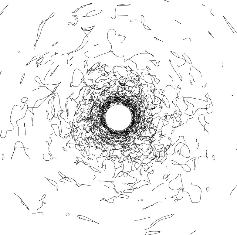
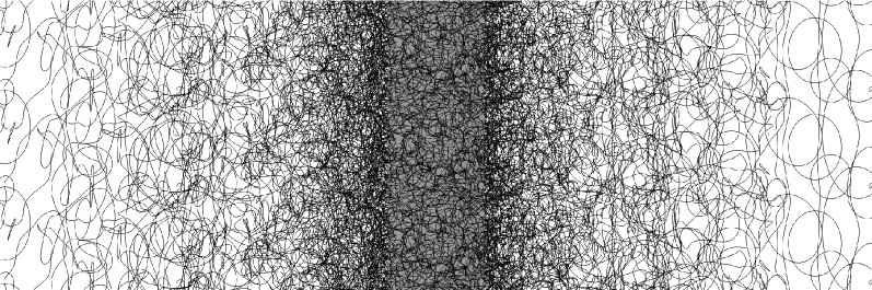
Figure 5: Configuration of quantized vortex lines in the statistically steady-state regime. Top: top view, bottom: side view.

Figure 5 illustrates the numerically simulated, statistically steady-state vortex tangle. It is interesting to notice that whereas in the inner regions the tangle is dense and apparently random, in the outer region large irregular vortex loops are visible which are oriented in the plane perpendicular to the radial direction of the heat flux. This effect can be understood in terms of the the dynamics of simpler circular vortex rings. Starting from the dense region, a vortex ring which travels in the outward radial direction gains energy from the normal fluid which flows in the same direction (radially out), slows down and becomes larger (thus gaining energy), until it collides with similar large loops, forming the large stationary vortex structures visible at the edge of Figure 5(top) near $r\approx 8a$.

To gain geometrical insight into the turbulence, at each instant of time we can divide the vortex configuration of vortex lines in two groups depending whether they are closed or attached to the boundary: ”vortex handles” (which are connected to the cylinder), and ”vortex loops” (distorted vortex rings) which are disconnected from the cylinder. Figure 6 displays the former in red and the latter in black. Figure 7 shows that the relative proportion of vortex handles is larger near the cylinder, whereas vortex loops are predominant far from the cylinder.

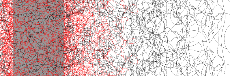
Figure 6: Enlarged view of the vortex configuration near the cylinder. Vortex handles (which are connected to the cylinder) are plotted in red, vortex loops (which are disconnected) are plotted in black.

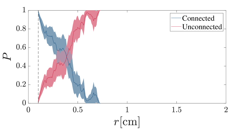
Figure 7: Relative proportion, $P$, of vortex loops (disconnected from the cylinder, pink) and vortex handles (connected to the cylinder, blue) as a function of radial distance, $r$. The coloured bands represent one standard deviation after time-averaging in the statistically stead-state regime.

It is interesting to analyse the properties of radial counterflow turbulence and compare them quantitatively to traditional counterflow turbulence in a channel. From our numerical solution we calculate the local average vortex line density in the statistically steady state regime as follows: we divided the flow domain for $0.1~{}{\rm cm}\leqslant r\leqslant 1~{}{\rm cm}$ into thin cylindrical shells of thickness $0.005\rm~{}cm$. Within each shell the vortex line density is then ensemble-averaged over a number of realizations of the initial vortex configuration. Figure 8 shows the result with the top panel plotted in the linear-linear scale and the bottom panel in the log-log scale. The large radial inhomogeneity of radial counterflow turbulence is apparent.

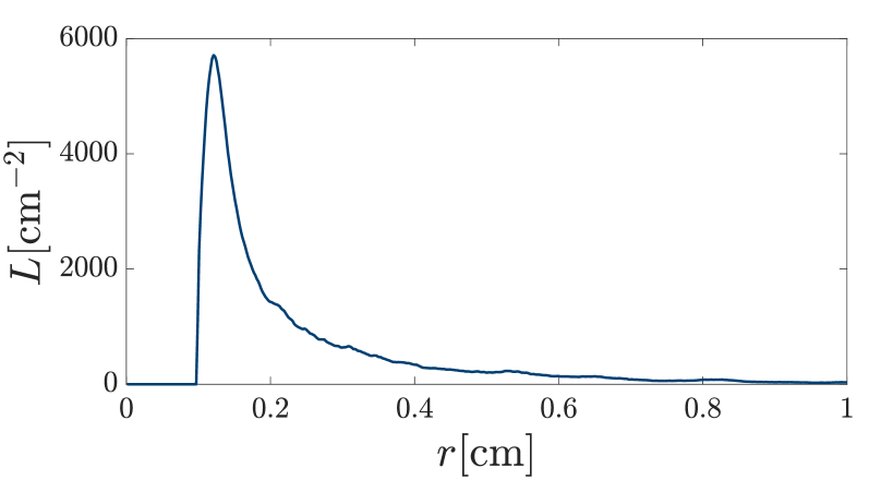
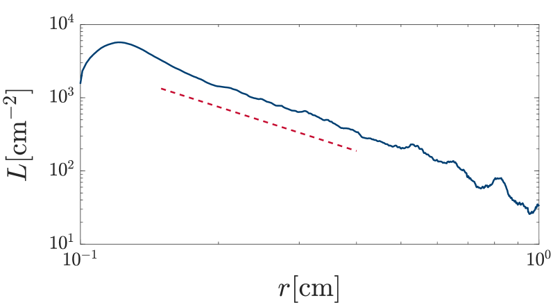
Figure 8: Top: radial distribution of the vortex line density $L(r)$ in the flow domain $r>a=0.1~{}\rm cm$ where $a$ is the radius of the cylinder. Bottom: $L(r)$ versus $r$ plotted on the log-log scale; the dashed (red) straight line shows the expected $r^{-2}$ scaling.

If the temperature is constant and the flow is steady, in the framework of the HVBK equations, the mass conservation equations reduce to ${\mbox{\boldmath$\nabla$}}\cdot{\bf{v}}_{s}=0$ and ${\mbox{\boldmath$\nabla$}}\cdot{\bf{v}}_{n}=0$. In the case of cylindrically symmetric radial counterflow these equations yield the radial distributions of the normal and superfluid velocities which scale with the radial coordinate as $r^{-1}$. Then, from the well-known Gorter-Mellink relation

$$L=\gamma^{2}{\mbox{$v_{ns}$}}^{2},$$ (6)

where ${\mbox{$v_{ns}$}}=|{\bf{v}}_{n}-{\bf{v}}_{s}|$ is the counterflow velocity and $\gamma=\gamma(T)$ is a temperature-dependent constant (see e.g. Refs. Adachi ; Kondaurova ), we expect that the vortex line density scales as $L\sim r^{-2}$. As seen from the bottom panel of Figure 8, at distances larger than about half a cylinder’s radius from the surface, the vortex line density behaves reasonably close to $\sim r^{-2}$ indeed, although some deviation from this scaling is apparent. This deviation is most likely due to the well-known observation that Eq. (6) should also include the so-called intercept velocity, $v_{i}$, and hence be written in a slightly different form Tough :

$$L=\gamma^{2}({\mbox{$v_{ns}$}}-v_{i})^{2}.$$ (7)

The intercept velocity is typical of turbulence at low counterflow velocities, corresponding to rather dilute vortex tangles Tough . Calculated from our numerical solution, the local average vortex line density as a function of the radially dependent counterflow velocity ${\mbox{$v_{ns}$}}={\mbox{$v_{n}$}}-{\mbox{$v_{s}$}}$ is shown in Figure 9. Within the interval of counterflow velocities roughly corresponding to the flow region where the line density is fully saturated, the behavior of the vortex line density is close note2 to the expected scaling $L\propto{\mbox{$v_{ns}$}}^{2}$, although some deviation from this scaling is apparent at low velocities. Note that our numerical results allow us to estimate the intercept velocity as $v_{i}\approx 0.002~{}\rm cm/s$, a value that is one order of magnitude smaller than that reported in Ref. Kondaurova (see also references therein) for counterflow in straight channels.

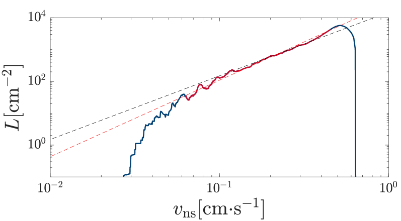
Figure 9: Vortex line density as a function of the counterflow velocity. The black dashed line shows the scaling $L\propto{\mbox{$v_{ns}$}}^{2}$, in good agreement with our data. The red dashed line shows the best fitnote2 , which is $L\propto{\mbox{$v_{ns}$}}^{2.4}$.

Finally, we measure the anisotropy of the turbulence as a function of radius using the anisotropy parameters of Schwarz Schwarz1988 :

$$I_{\parallel}=\frac{1}{\Lambda}\int_{\mathcal{L}}\left[1-(\mathbf{s}^{\prime}\cdot\hat{\mathbf{r}}_{\parallel})^{2}\right]d\xi,$$ (8)

$$I_{\perp}=\frac{1}{\Lambda}\int_{\mathcal{L}}\left[1-(\mathbf{s}^{\prime}\cdot\hat{\mathbf{r}}_{\perp})^{2}\right]d\xi,$$ (9)

where $\hat{\mathbf{r}}_{\parallel}$ and $\hat{\mathbf{r}}_{\perp}$ are unit vectors, respectively parallel and perpendicular to the direction of the counterflow velocity. Schwarz’s anisotropy parameters satisfy $I_{\parallel}/2+I_{\perp}=1$. If the vortex lines are aligned in the plane perpendicular to the counterflow direction, then $I_{\parallel}=1$ and $I_{\perp}=1/2$, while if the vortex lines are isotropic $I_{\parallel}=I_{\perp}=2/3$. Simulations of counterflow turbulence in a periodic box at $T=1.3~{}\rm K$ report Adachi $I_{\parallel}\approx 0.74$ in agreement with counterflow channel experiments ($I_{\parallel}\approx 0.77$).

In our case $\hat{\mathbf{r}}_{\parallel}$ is the outward radial unit vector. $I_{\parallel}$ and $I_{\perp}$ are estimated locally by calculating them over radial shells of width $0.01$ cm, with $\Lambda$ then being the total vortex line length within the shell and $\mathcal{L}$ being the vortex lines within the shell. Figure 10(top) shows that the turbulence is not isotropic anywhere. In the inner region very near the cylinder ($r\geq a$) and in the outer region ($r\geq 7a$), most vortex length lies in the plane perpendicular to the radial direction of the counterflow; in the intermediate region the anisotropy of radial counterflow is comparable to what is observed in standard channels. Figure 10(bottom) shows the average radius of curvature, $R$, of the vortex loops, defined locally as $R=1/|\bf{s}^{\prime\prime}|$. This geometrical property determines the dynamics (large vortex loops move slower than small loops). The graphs shows clearly that away from the cylinder there is a region dominated by large slow-moving vortex loops, consistently with Figure 5.

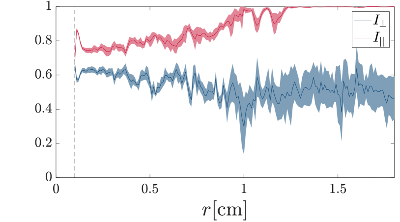
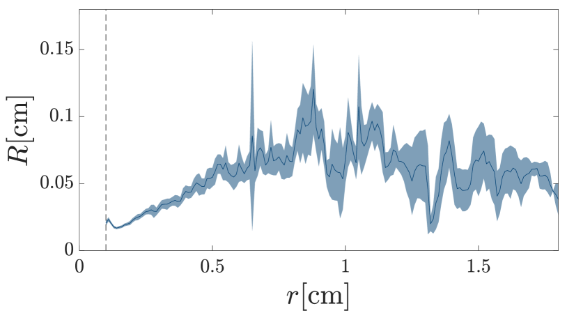
Figure 10: Top panel: anisotropy parameters of Schwarz Schwarz1988 , $I_{\parallel}$ (bottom, blue) and $I_{\perp}$ (top, pink), as a function of radial distance, $r$; the coloured bands represent one standard deviation. Bottom panel: average radius of curvature of the vortex lines, $R$, as a function of $r$; again the coloured band represents one standard deviation

.

V Conclusions

In our previous work Sergeev-EPL we have shown that, in the framework of the HVBK model applied to turbulence, the governing equations do not have a steady radial counterflow solution if the temperature of helium is assumed uniform throughout the whole flow domain. We have also shown that the vortex line density saturates to a steady state value only in the case where the radial distributions of temperature, normal fluid and superfluid densities, thermodynamic properties, and mutual friction coefficients are accounted for.

Using these  Sergeev-EPL findings, here we have developed a minimal model of turbulent radial counterflow which identifies the essential physics of the problem from the point of view of the vortex dynamics: the radial dependence of the friction. Our model assumes that the mutual friction coefficients are radially dependent and leaves the normal and superfluid densities and all thermodynamic properties constant throughout the flow domain. This radial dependence of the mutual friction coefficients (which mimics the changes calculated from the HVBK equations Sergeev-EPL ) takes place only within a relatively narrow region, about a half of the cylinder’s radius adjacent to the cylinder’s surface; outside this region the mutual friction coefficients retain constant values corresponding to the temperature in the bulk of helium. With this minimal model, the numerical simulations of turbulent counterflow based on the Biot-Savart law which we present here show that a dense layer of turbulent vortex lines forms near the heated cylinder and saturates to a statistical steady-state.

We have analysed the inhomogeneous vortex line density $L$ of this turbulent steady state and determined its anisotropy and its scalings with the radial coordinate, $r$, and with the counterflow velocity, $v_{ns}$. We have found scalings which are reasonably close to $L\propto r^{-2}$ and $L\propto{\mbox{$v_{ns}$}}^{2}$ expected from homogeneous counterflow turbulence in standard channels.

At present, a numerical model based on the Biot-Savart law that goes beyond the current minimal model and properly incorporates spatial variations of temperature together with temperature-dependent densities, thermodynamic properties, and mutual friction coefficients seems too ambitious, considering limitations of computing power. However, the identification of the spatial dependence of the mutual friction as the main physical mechanism responsible for the saturation of the vortex tangle to a statistically steady state, which is the main result of this paper, should help the study of thermal counterflow in the case of other non-trivial flow geometries. Moreover, the validity of Vinen’s scaling $L\propto{\mbox{$v_{ns}$}}^{2}$ in strongly inhomogeneous turbulence which we have directly verified in this work is going to help develop further the theory of inhomogeneous superfluid turbulence.

We acknowledge the support of the EPSRC (Engineering and Physical Sciences Research Council) grant EP/R005192/1.

References

- (1) W.F. Vinen, Mutual friction in a heat current in liquid helium II, Proc. Roy. Soc. A 240, 114; 240, 128; 242, 493; 243 400, (1957).
- (2) P. Švančara, P. Hrubcová, M. Rotter, and M. La Mantia, Visualization study of thermal counterflow of superfluid helium in the proximity of the heat source by using solid deuterium hydride particles, Phys. Rev. Fluids 3, 114701 (2018).
- (3) B. Mastracci, S. Bao, W. Guo, and W. F. Vinen, Particle tracking velocimetry applied to thermal counterflow in superfluid 4He: Motion of the normal fluid at small heat fluxes. Phys. Rev. Fluids 4, 083305 (2019).
- (4) S. Yui, M. Tsubota, and H. Kobayashi, Three-dimensional coupled dynamics of the two-fluid model in superfluid 4He: deformed velocity profile of normal fluid in thermal counterflow, Phys. Rev. Lett. 120, 155301 (2018).
- (5) L. Biferale, D. Khomenko, V. L’vov, A. Pomyalov, I. Procaccia, and G. Sahoo, Superfluid helium in three-dimensional counterflow differs strongly from classical flows: anisotropy on small scales. Phys. Rev. Lett. 122, 144501 (2019).
- (6) A.W. Baggaley and J. Laurie, Thermal counterflow in a periodic channel with solid boundaries. J. Low Temp. Phys. 178, 35 (2015).
- (7) D. Duri, C. Baudet, J.-P. Moro, P.-E. Roche, and P. Diribarne, Hot-wire anemometry for superfluid turbulent coflows, Rev. Sci. Instruments 86, 025007 (2015).
- (8) The results which we present here do not apply directly to current anemometry experiments, as in these experiments the temperature may exceed and in the lambda region the vortex line density would become to large for our simulations.
- (9) J. T. Tough, Superfluid turbulence, in Progress in Low Temperature Physics, edited by D. F. Brewer, Vol. 8 (North Holland, Amsterdam, 1982), p. 133.
- (10) K. W. Schwarz, Three-dimensional vortex dynamics in superfluid 4He: Homogeneous superfluid turbulence, Phys. Rev. B 38, 2398 (1988).
- (11) R. J. Donnelly and C. F. Barenghi, The observed properties of liquid helium at the saturated vapor pressure, J. Phys. Chem. Ref. Data 27, 1217 (1998).
- (12) H. Adachi, S. Fujiyama, and M. Tsubota, Steady-state counterflow turbulence: Simulation of vortex filaments using the full Biot-Savart law, Phys. Rev. B 81, 104511 (2010).
- (13) More precisely, to define we monitor the vortex length within the fifth shell around the cylinder, as defined in the caption of Figure 4.
- (14) A. W. Baggaley and C. F. Barenghi, Tree method for quantum vortex dynamics, J. Low Temp. Phys. 166, 3 (2012).
- (15) A. W. Baggaley, The sensitivity of the vortex filament method to different reconnection models, J. Low Temp. Phys. 168, 18 (2012).
- (16) J. Laurie and A. W. Baggaley, Reconnection dynamics and mutual friction in quantum turbulence, J. Low Temp. Phys. 180, 82 (2015).
- (17) K. W. Schwarz, Turbulence in superfluid helium: Steady homogeneous counterflow, Phys. Rev. B 18, 245 (1978).
- (18) E. Varga, Peculiarities of spherically symmetric counterflow, J. Low Temp. Phys. 196, 28 (2019).
- (19) Y. A. Sergeev and C. F. Barenghi, Turbulent radial thermal counterflow in the framework of the HVBK model, Europhys. Lett. 128, 26001 (2019).
- (20) I. M. Khalatnikov, An Introduction to the Theory of Superfluidity (Benjamin, New York – Amsterdam, 1965).
- (21) P.-E. Roche, C. F. Barenghi, and E. Leveque, Quantum turbulence at finite temperature: the two-fluids cascade. Europhys. Letters 87, 54006 (2009).
- (22) A.W. Baggaley, J. Laurie, and C.F. Barenghi, Vortex density fluctuations, energy spectra and vortical regions in superfluid turbulence. Phys. Rev. Letters 109, 205303 (2012).
- (23) Kondaurova L., L’vov V., Pomyalov A. and Procaccia I., Structure of a quantum vortex tangle in 4He counterflow turbulence. Phys. Rev. B 89, 014502 (2014).
- (24) A slightly better fit (shown by the red dashed line in Figure 9) is provided by with cm/s corresponding to the region .