Event Classification with Quantum Machine Learning in High-Energy Physics

Abstract

We present studies of quantum algorithms exploiting machine learning to classify events of interest from background events, one of the most representative machine learning applications in high-energy physics. We focus on variational quantum approach to learn the properties of input data and evaluate the performance of the event classification using both simulators and quantum computing devices. Comparison of the performance with standard multi-variate classification techniques based on a boosted-decision tree and a deep neural network using classical computers shows that the quantum algorithm has comparable performance with the standard techniques at the considered ranges of the number of input variables and the size of training samples. The variational quantum algorithm is tested with quantum computers, demonstrating that the discrimination of interesting events from background is feasible. Characteristic behaviors observed during a learning process using quantum circuits with extended gate structures are discussed, as well as the implications of the current performance to the application in high-energy physics experiments.

1 Introduction

The field of particle physics has been recently driven by large experiments to collect and analyze data produced in particle collisions occurred using high-energy accelerators. In high-energy physics (HEP) experiments, particles created by collisions are observed by layers of high-precision detectors surrounding collision points, producing a large amount of data. The large data volume has motivated the use of machine learning (ML) techniques in many aspects of experiments to improve their performances (see, e.g, hepmllivingreview for a living review of ML techniques to particle physics). In addition, computational resources are expected to be reduced for specific tasks by adopting relatively new techniques such as ML. This will continue over next decades; for example, a next-generation proton-proton collider, called High-Luminosity Large Hadron Collider (HL-LHC) ApollinariG.:2017ojx ; Evans:2008zzb , at CERN  is expected to deliver a few exabytes of data every year and requires very large computing resources for the data processing. Quantum computing (QC), on the other hand, has been evolving rapidly over the past years, with a promise of a significant speed-up or reduction of computational resources in certain tasks. Early attempts to use QC for HEP have been made, e.g, on data analysis Mott:2017xdb ; Zlokapa:2019lvv , identification of charged particle trajectories Shapoval:2019txi ; Bapst:2019llh ; Zlokapa:2019tkn ; Tuysuz:2020ocw , reconstruction of particle collision points Das:2019hrw and particle spray called jets Wei:2019rqy , as well as the simulation of event generation called parton shower Bauer:2019qx ; Bauer:2019qxa . The techniques developed in HEP are also adapted to QC, e.g, the unfolding techniques for physics measurement are applied to QC in Refs. Cormier:2019kcq ; Bauer:2019uf . Among these attempts, the quantum machine learning (QML) is considered as one of the QC algorithms that could bring quantum advantages over classical methods, as discussed in literatures, e.g, Preskill2018quantumcomputingin .

Most frequently-used ML technique in HEP data analysis is the discrimination of events of interest, e.g, signal events originating from new physics beyond the Standard Model of particle physics, from background events. In this paper, we have investigated the application of QML techniques to the task of the event classification in HEP data analysis. To our knowledge, the first attempt to utilize QC for HEP data analysis is performed in Ref. Mott:2017xdb for the classification of the Higgs boson using quantum annealing Johnson2011Quantum .

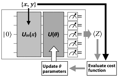
Figure 1: Representative variational quantum circuit used for the event classification in this study. $\{\boldsymbol{x},\boldsymbol{y}\}$ is a set of pairs composed of an input data $\boldsymbol{x}$ and an input label $\boldsymbol{y}$ (desired output value). $\langle Z\rangle$ is an output from the quantum circuit. The components of the circuit and their roles are explained in the text.

We focus on QML algorithms developed for gate-based quantum computer, in particular the algorithms based on variational quantum circuit Peruzzo2014vqe . In the variational circuit approach, the classical input data are encoded into quantum states and a quantum computer is used to obtain and measure the quantum states which vary with tunable parameters. Exploiting a complex Hilbert space that grows exponentially with the number of “quantum bits” (or qubits) in quantum computer, the representational ability of the QML is far superior to classical ML that grows only linearly with the number of classical bits. This motivates the application of ML techniques to quantum computer, which could lead to an advantage over the classical approach. The optimization of the parameters is performed using classical computer, therefore the variational method is considered to be suitable for the present quantum computer, which has difficulty in processing deep quantum circuits due to limited quantum coherence. Practically, actual performance of the variational quantum algorithm depends on the implementation of the algorithm and the properties of the QC device. The primary aim of this paper is to demonstrate the feasibility of ML for the event classification in HEP data analysis using gate-based quantum computer.

First, the variational quantum algorithms are described in Sect. 2, followed by the classical approaches that are used for the comparison. Section 3 discusses the experimental setup used in the study, including the dataset, software simulator and quantum computer. Results of the experiments are discussed in Sect. 4, followed by discussions on several observations about the performance of the quantum algorithms in Sect. 5. We conclude the studies in Sect. 6.

2 Algorithms

2.1 Variational Quantum Approaches

In this study we consider an approach based on variational quantum circuit with tunable parameters Peruzzo2014vqe . The quantum circuit used in this algorithm is constr-ucted, as shown in Fig. 1, using three components: 1) quantum gates to encode classical input data $\boldsymbol{x}$ into quantum states (denoted as $U_{\text{in}}(\boldsymbol{x})$), 2) quantum gates to produce output states used for supervised learning (denoted as $U(\boldsymbol{\theta})$) and 3) measurement gates to obtain output values from the circuit, that are subsequently compared with the corresponding input labels $\boldsymbol{y}$. In this study, the measurement is performed 1,024 times on each event with the Pauli-$Z$ operators and the average value of the measurements is used for improving the statistical accuracy. For the classification of events into two categories, the first two qubits are typically measured. The $U(\boldsymbol{\theta})$ gates used in 2) are parameterized such that they are optimized to model input training data by iterating the computational processes of 1)–3) by $N_{\text{iter}}$ times and tuning the parameters $\boldsymbol{\theta}$. The parameter tuning is performed using a classical computer by minimizing a cost function, which is defined such that a difference between the input labels $\boldsymbol{y}$ and the measured values $\langle Z\rangle$ can be quantified. The optimized $U(\boldsymbol{\theta})$ circuit with the tuned parameters is used, with the same $U_{\text{in}}(\boldsymbol{x})$ gates, to classify unseen data for testing. The $U_{\text{in}}(\boldsymbol{x})$ and $U(\boldsymbol{\theta})$ are often built by using a same set of quantum gates with different parameters multiple times to enhance the representational ability of the data. The numbers of the repetition used for the $U_{\text{in}}(\boldsymbol{x})$ and $U(\boldsymbol{\theta})$ are denoted by $N_{\text{in}}^{\text{depth}}$ and $N_{\text{var}}^{\text{depth}}$, respectively.

In this study, we use two implementations of the variational quantum algorithms, called Quantum Circuit Learning (QCL) Mitarai_2018 and Variational Quantum Classification (VQC) Havlcek2019SupervisedLW . The QCL is used for testing the performance of the variational quantum algorithm on simulator. The VQC is used for testing the algorithm on both real quantum computer and simulator with small samples.

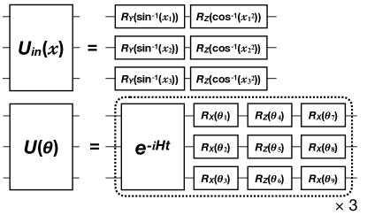
Figure 2: $U_{\text{in}}(\boldsymbol{x})$ and $U(\boldsymbol{\theta})$ circuits used in this study for the QCL algorithm.

2.1.1 Quantum Circuit Learning

A QCL circuit used in this study for the 3-variable classification is shown in Fig. 2. The $U_{\text{in}}(\boldsymbol{x})$ in QCL is characterized by the series of single-qubit rotation gates $R_{Y}$ and $R_{Z}$ Mitarai_2018 . The angles of the rotation gates are obtained from the input data $\boldsymbol{x}$ to be $\sin^{-1}(\boldsymbol{x})$ and $\cos^{-1}(\boldsymbol{x}^{2})$, respectively. The input data are needed to be normalized within the range [$-1$, $1$] by scaling linearly using the maximum and minimum values of the input variables. The normalization is performed separately for the training and testing samples to avoid data beyond the [$-1$, $1$] range. In this case, the classification performance is slightly suboptimal for the testing sample. The effect is however checked to be small by comparing the performance with the case where the testing sample is normalized with the scaling derived from the training sample and clipped to [$-1$, $1$]. The $U(\boldsymbol{\theta})$ is constructed using a time-evolution gate, denoted as $e^{-iHt}$, with the Hamiltonian $H$ of an Ising model with random coefficients (for creating entanglement between qubits) and the series of $R_{X}$, $R_{Z}$ and $R_{X}$ gates with angles as parameters. The nominal $N_{\text{var}}^{\text{depth}}$ value is set to 3 after optimization studies. This results in 27 parameters in total for the 3-variable case. The structure for the 5- and 7-variable circuits is the same as the 3-variable case, leading to the total parameters of 45 and 63, respectively. The measurement is performed on the first two qubits using the Pauli-$Z$ operators, and the outcome of the measurement is fed into the cost function via softmax. The cost function is defined using a cross-entropy function in scikit-learn package scikit-learn , and the minimization of the cost function is performed using COBYLA. See Mitarai_2018 for more details about the implementation.

2.1.2 Variational Quantum Classification

Figure 3 shows a VQC circuit for the 3-variable classification used in this study. The $U_{\text{in}}(\boldsymbol{x})$ consists of a set of Hadamard gates and rotation gates with angles from the input data $\boldsymbol{x}$ (the latter is represented as $U_{\phi}(\boldsymbol{x})$ in the figure). The $U_{\phi}(\boldsymbol{x})$ is composed of single-qubit rotation gates of the form $U_{\phi_{\{k\}}}(\boldsymbol{x})=\exp{(i\phi_{\{k\}}(\boldsymbol{x})Z_{k})}$, a diagonal phase gate with the linear function of $\phi_{\{k\}}(\boldsymbol{x})=x_{k}$. This is identical to the one used in Ref. Havlcek2019SupervisedLW as the single-qubit gate (see Eq. (32) of the supplementary information of Ref. Havlcek2019SupervisedLW ), and is referred to as the“First Order Expansion” (FOE). The $U_{\phi}(\boldsymbol{x})$ is not repeated in this study unless otherwise stated, thus $N_{\text{in}}^{\text{depth}}=1$. The $U(\boldsymbol{\theta})$ part of the circuit is also taken from that in Havlcek2019SupervisedLW but simplified by not repeating a set of entangling gate ($U_{\text{ent}}$) and single-qubit rotation gates $R_{Y}$ and $R_{Z}$ (surrounded by the dashed box in Fig. 3). The $U_{\text{ent}}$ is implemented using the Hadamard and CNOT gates, as in Fig. 3. The total number of $\boldsymbol{\theta}$ parameters is 12 (20, 28) for the 3 (5, 7)-variable classification. The measurement is performed on all the qubits using the Pauli $Z$ operators, and the measured outcomes are fed into the cost function. The cost function for the VQC algorithm is a cross-entropy function and the minimization is performed using COBYLA as well.

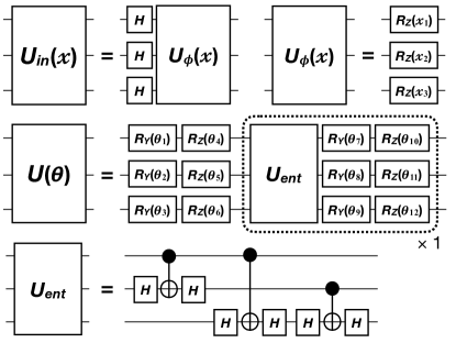
Figure 3: $U_{\text{in}}(\boldsymbol{x})$ and $U(\boldsymbol{\theta})$ circuits used in this study for the VQC algorithm.

2.2 Classical Approaches

The ML application to the classification of events has been widely attempted in HEP data analyses. Among others, a Boosted Decision Tree (BDT) in the TMVA framework Speckmayer_2010 is one of the most commonly used algorithms. A neural network (NN) is another class of multivariate analysis methods, and an algorithm with a deep neural network (DNN) has been proven to be powerful for modelling complex multi-dimensional problems. We use BDT and DNN as benchmark tools for comparison with the performance of the variational quantum algorithms.

In this study we use the TMVA package 4.2.1 for the BDT and the Keras 2.1.6 with TensorFlow 1.8.0 backend for the DNN. The BDT and DNN parameters used are summarized in Table 1. The maximum depth of the decision tree (MaxDepth) and the number of trees in the forest (NTrees) vary with the number of events used in the training ($N_{\text{event}}^{\text{train}}$) to avoid over-training. The DNN model is a fully-connected feed-forward network composed of 2–6 hidden layers with 16–256 nodes each. The numbers of hidden layers and nodes per layer are varied according to $N_{\text{event}}^{\text{train}}$ to avoid over-training.

Table 1: Parameter settings for the BDT and DNN used in this study. The definitions of the BDT parameters are documented in Ref. Speckmayer_2010 .

BDT Parameter	Value
BoostType	Grad
NTrees	10 ($N_{\text{event}}^{\text{train}}=0.1\text{K}$),
	100 ($0.5\text{K}\leq N_{\text{event}}^{\text{train}}\leq 10\text{K}$),
	1000 ($N_{\text{event}}^{\text{train}}\geq 50\text{K}$)
MaxDepth	1 ($N_{\text{event}}^{\text{train}}\leq 1\text{K}$),
	2 ($5\text{K}\leq N_{\text{event}}^{\text{train}}\leq 100\text{K}$),
	3 ($N_{\text{event}}^{\text{train}}\geq 200\text{K}$)
nCuts	20
MinimumNodeSize	2.5%
UseBaggedBoost	True
BaggedSampleFraction	0.5

DNN Parameter	Value
Layer Type	Dense
Number of hidden layers	2 ($N_{\text{event}}^{\text{train}}=0.1\text{K}$ or 1K),
	3 ($N_{\text{event}}^{\text{train}}=0.5\text{K}$),
	4 ($5\text{K}\leq N_{\text{event}}^{\text{train}}\leq 100\text{K}$),
	6 ($N_{\text{event}}^{\text{train}}\geq 200\text{K}$)
Number of nodes per	16 ($0.1\text{K}\leq N_{\text{event}}^{\text{train}}\leq 0.5\text{K}$),
hidden layer	64 ($1\text{K}\leq N_{\text{event}}^{\text{train}}\leq 10\text{K}$),
	128 ($50\text{K}\leq N_{\text{event}}^{\text{train}}\leq 100\text{K}$),
	256 ($N_{\text{event}}^{\text{train}}\geq 200\text{K}$)
Activation function	rectified linear unit
Optimizer	Adam
Learning rate	0.001
Batch size	None ($N_{\text{event}}^{\text{train}}\leq 10\text{K}$),
	2048 ($N_{\text{event}}^{\text{train}}\geq 50\text{K}$)
Batch normalization	No
Number of epochs	100 with early stopping

3 Experimental Setup

Our experimental test of the variational quantum algorithms is performed using both simulators of quantum computers and real quantum computers available via the IBM Q Network IBMQ . As a benchmark scenario for the HEP data analysis, we consider a problem of discriminating events with Supersymmetry (SUSY) particles from the most representative background events.

3.1 Dataset

We use the “SUSY Data Set” available in the UC Irvine Machine Learning Repository Dua:2019 , which was prepared for studies of Ref. Baldi:2014kfa . The signal process, labelled true, targets a chargino-pair production via a Higgs boson. Each chargino decays into a neutralino that escapes detection and a $W$-boson that subsequently decays into a charged lepton and a neutrino, resulting in a final state with two charged leptons and a missing transverse momentum. The background process, labelled false, is a $W$-boson pair production ($WW$) with each $W$-boson decaying into a charged lepton and a neutrino. Therefore, both the signal and background processes have the same final state. Monte Carlo simulation is used to produce events of these processes as described in Baldi:2014kfa .

In our main studies a small fraction of the data is used because the process of the full data (5 million events) with the quantum algorithms requires significant computing resources. For the comparison of the quantum and classical MLs, five sets of data containing 100, 500, 1,000, 5,000 and 10,000 events are used for training and other five sets of data with the same number of events for testing. For the classical MLs, additional four sets of data containing 50,000, 100,000, 200,000 and 500,000 events are used to study the dependence on the sample size.

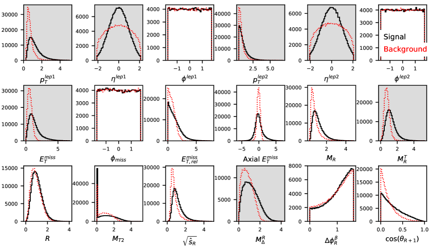
Figure 4: Normalized distributions of input variables for SUSY signal (solid histograms) and background (dashed histograms). The first nine variables up to $E_{\text{T, rel}}^{\text{miss}}$ are low-level features and the last nine are high-level ones. The main variables used in the study are highlighted in grey on the background while all the variables are considered for the DNN and BDT, as discussed in the text.

The dataset contains 18 variables characterizing the properties of the SUSY signal and $WW$ background events, ranging from low-level variables such as lepton transverse momenta to high-level variables such as those reflecting the kinematics of $W$-bosons and/or charginos (detailed in Baldi:2014kfa ). Figure 4 shows the normalized distributions of the 18 variables for the signal and background events. Among those, the following 3, 5 and 7 variables, which are quoted as $N_{\text{var}}=3$, 5 and 7 later, are considered in the main study:

   3 variables:

$p_{\text{T}}^{\text{lep1}}$, $p_{\text{T}}^{\text{lep2}}$ and $E_{T}^{\text{miss}}$,

   5 variables:

3 variables above, $M_{R}^{T}$, $M_{\Delta}^{R}$,

   7 variables:

5 variables above, $\eta^{\text{lep1}}$, $\eta^{\text{lep2}}$.

The choice of these variables is made as follows: first, the combination of 3 variables is determined by testing different combinations of the variables using the DNN algorithm and taking the one with the highest AUC (area under ROC curve) value. Starting with the selected variables of $N_{\text{var}}=3$, more variables are sequentially added and determined in the same way for $N_{\text{var}}=5$ and 7. In addition, all the 18 variables are used for evaluating the best performance which the classical MLs can reach (Sect. 4.1).

3.2 Simulator

We use quantum circuit simulators to evaluate the performance of the quantum algorithms. The QCL circuit is implemented using Qulacs 0.1.8 Qulacs , a fast quantum circuit simulator implemented in C++, with Python 3.6.5 and gcc 7.3.0, and the performance is evaluated on cloud Linux servers managed by OpenStack at CERN. The Qulacs supports the use of GPU, but it is not exploited in this study. The VQC circuit is implemented using Aqua 0.6.1 in the Qiskit 0.14.0 Qiskit , a quantum computing software development framework (Qiskit Aq-ua framework). The VQC performance is evaluated using a QASM simulator on a local machine as well as real quantum computer explained in the next section. No wall-time comparison is made between the simulators in this study.

The Qulacs simulator has capability of executing the variational quantum algorithm with more variables or more data events than the QASM simulator. This allows us to evaluate the performance of the quantum algorithm in more realistic settings.

3.3 Quantum Computer

We use the 20-qubit IBM Q Network quantum computers, called Johannesburg johannesburg and Boeblingen boeblingen , for evaluating the VQC performance. The quantum computers are accessed using the QuantumInstance class in the Qiskit Aqua framework. The $U_{\text{in}}(\boldsymbol{x})$ part of the VQC circuit (Fig. 3) is created separately for each event because the $U_{\phi}(\boldsymbol{x})$ gates depend on the input data $\boldsymbol{x}$. For the training and testing, we use 40 events each, composed of 20 signal and 20 background events. The $\boldsymbol{\theta}$ parameters are determined by iterating the training process as explained in Sect. 2.1. The $N_{\text{iter}}$ is set to 100 unless otherwise stated.

4 Results

4.1 Qulacs Simulator

First, the classification performance of the QCL algorithm evaluated using the Qulacs simulator is compared with those of the BDT and DNN. Due to a significant increase of the computational resources with $N_{\text{var}}$ for the QCL (discussed in Sect. 5.4), the $N_{\text{var}}$ is considered only up to 7.

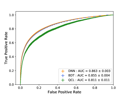
Figure 5: ROC curves obtained from the test sample for the BDT, DNN and QCL algorithms with $N_{\text{var}}=7$ and $N_{\text{event}}^{\text{train}}=10,000$. The error bands correspond to the standard deviations of the values obtained by repeating the calculation over the training and test samples.

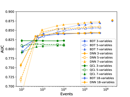
Figure 6: Average AUC values (calculated from the test samples) as a function of the training sample size for the BDT, DNN and QCL algorithms with $N_{\text{var}}=3$ (circles), 5 (squares) and 7 (triangles). For the BDT and DNN, the average AUC values for the training sample of 2,000,000 events and 18 variables are also shown with the plus markers. The error bars represent the standard deviations of the average AUC values. The BDT and DNN points are slightly shifted horizontally from the nominal $N_{\text{event}}^{\text{train}}$ values to avoid overlapping.

Figure 5 shows ROC curves in the testing for the three algorithms with $N_{\text{var}}=7$ and $N_{\text{event}}^{\text{train}}=10,000$, and Figure 6 shows the comparisons of the AUC values as a function of $N_{\text{event}}^{\text{train}}$ for $N_{\text{var}}=3$, 5 and 7. For each algorithm, a single AUC value is obtained from a test sample after each training, and the calculation is repeated 100 (30) times at $N_{\text{event}}^{\text{train}}\leq 10,000$ ($50,000\leq N_{\text{event}}^{\text{train}}\leq 500,000$). The center and the width of each curve in Fig. 5 correspond to the average value and the standard deviation of the true/false positive rates obtained from the repeated calculations over the training and test samples. Shown in Fig. 6 is the average of the resulting AUC values and the standard deviations of the average. As expected, it is apparent from the BDT and DNN curves that the performance of these two algorithms improves rapidly with increasing $N_{\text{event}}^{\text{train}}$ and then flattens out. The BDT works well over the entire $N_{\text{event}}^{\text{train}}$ range while the DNN performance appears to improve faster at very small $N_{\text{event}}^{\text{train}}$ and exceed BDT at $N_{\text{event}}^{\text{train}}$ beyond $\sim 1,000$. In the case of $N_{\text{var}}=7$ and $N_{\text{event}}^{\text{train}}=500,000$, the AUC values are $0.8729\pm 0.0003$ for the DNN and $0.8696\pm 0.0006$ for the BDT. When using all the 18 variables with 2,000,000 events for the training and testing each, the average AUC value from only five trials is $0.8772\pm 0.0004$ ($0.8750\pm 0.0004$) for the DNN (BDT).

The performance of the QCL algorithm is characterized by the relatively flat AUC values regardless of $N_{\text{event}}^{\text{train}}$. Increasing the $N_{\text{var}}$ appears to degrade the performance if the $N_{\text{event}}^{\text{train}}$ is fixed, and the same behavior is also seen for the DNN with $N_{\text{event}}^{\text{train}}\leq 500$ (not clearly visible for the BDT). Further studies show that the QCL performance of the flat AUC value and the degradation with increasing $N_{\text{var}}$ is related to the choice of the variables: the $N_{\text{var}}=3$ variables used have sufficient information for the QCL algorithm to discriminate the signal from background, and no positive impact is seen on the performance by adding more variables or more events. However, it is seen that the performance improves by adding them if different combinations of the variables are selected. The DNN algorithm overcomes the degradation and eventually improves the performance with increasing $N_{\text{var}}$ by using more data. Investigating how the QCL algorithm behaves with more data is a future subject. Nevertheless, for the $N_{\text{var}}$ and $N_{\text{event}}^{\text{train}}$ ($\leq$ 10,000) ranges considered all the three algorithms have a comparable discriminating power with the AUC values of 0.80–0.85.

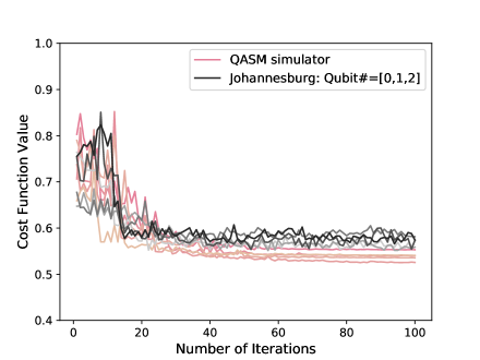
Figure 7: Evolution of the cost function value in the training of the VQC algorithm with $N_{\text{var}}=3$ and $N_{\text{event}}^{\text{train}}=40$. Shown are the cost function values observed in 5 training trials for quantum computer and QASM simulator.

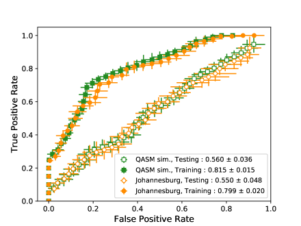
Figure 8: ROC curves in the training and testing of the VQC algorithm with $N_{\text{var}}=3$ and $N_{\text{event}}^{\text{train}}=40$. Shown are the ROC curves (averaged over five trials in the training or testing) for quantum computer and QASM simulator. The size of the markers represents the standard deviation of the trials. The values in the legend give the average AUC values and the standard deviations.

4.2 Quantum Computer and QASM Simulator

The VQC algorithm with $N_{\text{var}}=3$ has been tested on the 20-qubit IBM Q Network quantum computers and the QASM simulator, as explained in Sect. 3.3. The present study focuses only on the classification accuracy with the real quantum computer. Figure 7 shows the values of the cost function in the training as a function of $N_{\text{iter}}$ for both the quantum computer and the simulator. For each of the quantum computer and the simulator, the training is repeated five times over the same set of events and their cost-function values are shown. When running the algorithm on the quantum computer, the first three hardware qubits [0, 1, 2] are used IBMQConfMap . The figure shows that both the quantum computer and the simulator have reached the minimum values in the cost function after iterating about 50 times. However, the cost values for the quantum computer are constantly higher and more fluctuating after reaching the minimum values.

Table 2: AUC values in the testing and training for the VQC algorithm running the QASM simulator. The training condition is fixed to $N_{\text{var}}=3$ and $N_{\text{iter}}=100$ for all $N_{\text{event}}^{\text{train}}$ cases. The uncertainties correspond to the standard deviations of the average AUC values over the trials.

$N_{\text{event}}^{\text{train}}$ ($=N_{\text{event}}^{\text{test}}$)	Testing	Training
40	$0.555\pm 0.032$	$0.813\pm 0.012$
70	$0.716\pm 0.037$	$0.741\pm 0.022$
100	$0.708\pm 0.039$	$0.761\pm 0.025$
200	$0.812\pm 0.012$	$0.741\pm 0.014$
500	$0.779\pm 0.008$	$0.796\pm 0.007$
1000	$0.779\pm 0.008$	$0.789\pm 0.005$

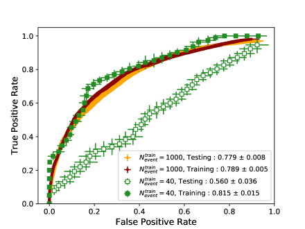
Figure 9: ROC curves in the training and testing of the VQC algorithm with $N_{\text{event}}^{\text{train}}=40$ and 1,000 for $N_{\text{var}}=3$. Shown are the ROC curves (averaged over five trials in the training or testing) for QASM simulator. The size of the markers or the band width represent the standard deviation of the trials. The values in the legend give the average AUC values and the standard deviations.

The ROC curves for the quantum computer and the simulator obtained from the training and testing samples are shown in Fig. 8, averaged over the five trials of the training or testing. The AUC values for the testing samples are considerably worse than those for the training ones because of the small sample sizes. This has been checked by increasing the $N_{\text{event}}^{\text{train}}$ from 40 to 70, 100, 200, 500 and 1,000 for the simulator (Table 2). As seen in the table, the over-training largely disappears as the sample sizes increase. Figure 9 shows the ROC curves from the simulator for the two sample sizes of $N_{\text{event}}^{\text{train}}=40$ and 1,000, confirming that the over-taining is not significant for the latter.

The AUC values are consistent between the quantum computer and the simulator within the standard deviation (Fig. 8), but the simulator results are considered to be systematically better because the input samples are identical. In Table 3, the VQC results are compared with the QCL being executed at the same condition, i.e, $N_{\text{var}}=3$, $N_{\text{event}}^{\text{train}}=40$ and $N_{\text{iter}}=100$. The QCL results vary with the depth of the $U(\boldsymbol{\theta})$ circuit (the nominal $N_{\text{var}}^{\text{depth}}$ is 3), but they agree with the VQC results within relatively large uncertainties. Summarized in Table 3 are the AUC values and their standard deviations in the training of the VQC and QCL algorithms.

Table 3: AUC values in the training for the VQC and QCL algorithms running on quantum computers and simulators. The QCL results are given for $N_{\text{var}}^{\text{depth}}=1$ and 3. The training condition is fixed to $N_{\text{var}}=3$, $N_{\text{event}}^{\text{train}}=40$ and $N_{\text{iter}}=100$ for both algorithms. The uncertainties correspond to the standard deviations of the average AUC values over the trials.

	Device/Condition	AUC
VQC	Johannesburg	$0.799\pm 0.020$
	Boeblingen	$0.807\pm 0.010$
	QASM simulator	$0.815\pm 0.015$
QCL	Qulacs simulator ($N_{\text{var}}^{\text{depth}}=1$)	$0.768\pm 0.082$
	Qulacs simulator ($N_{\text{var}}^{\text{depth}}=3$)	$0.833\pm 0.063$

5 Discussion

5.1 Performance with different QCL models

As seen in Fig. 6, the QCL performance stays approximately flat in $N_{\text{event}}^{\text{train}}$ and gets slightly worse when increasing the $N_{\text{var}}$ at fixed $N_{\text{event}}^{\text{train}}$. Since the computational resources needed to explore the QCL model with more variables ($N_{\text{var}}>\approx 10$) or larger sample sizes ($N_{\text{event}}^{\text{train}}>10$K) are beyond our capacity (Sect. 5.4), understanding the behavior and the dependence on the $N_{\text{var}}$ or $N_{\text{event}}^{\text{train}}$ is a subject for future study.

To investigate a possibility that the QCL performance could be limited by insufficient flexibility of the circuit used (Fig. 2), alternative QCL models with the $U(\boldsymbol{\theta})$ circuit of $N_{\text{var}}^{\text{depth}}=5$ or 7, instead of 3, are tested. This changes the AUC values by 1-2% at most for the $N_{\text{event}}^{\text{train}}$ of 100 or 1,000 events, which is negligible compared to the statistical fluctuation. Another type of QCL circuit is also considered by modifying the $U_{\text{in}}(\boldsymbol{x})$ to include 2-qubit gates for creating entanglement, as shown in Fig. 10 (as motivated by the Second Order Expansion in VQC; see Sect. 5.2). It turns out that the QCL with the new $U_{\text{in}}(\boldsymbol{x})$ does not increase the AUC values when the $U(\boldsymbol{\theta})$ is fixed to the original model with $N_{\text{var}}^{\text{depth}}=3$ in Fig. 2. On the other hand, the new $U_{\text{in}}(\boldsymbol{x})$ appears to improve the performance by 5–10% with respect to the original $U_{\text{in}}(\boldsymbol{x})$ when $N_{\text{var}}^{\text{depth}}$ is set to 1. This indicates that a more complex structure in the $U_{\text{in}}(\boldsymbol{x})$ could help improve the performance when the $U(\boldsymbol{\theta})$ is simplified. However, the performance of the new $U_{\text{in}}(\boldsymbol{x})$ with $N_{\text{var}}^{\text{depth}}=1$ is still considerably worse than the nominal QCL model in Fig. 2.

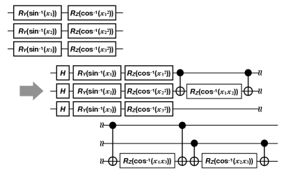
Figure 10: Nominal and alternative $U_{\text{in}}(\boldsymbol{x})$ circuits used in QCL to check impact on the performance.

5.2 Performance with different VQC models

The VQC circuit used in this study (Fig. 3) is simplified with respect to the one used in Ref. Havlcek2019SupervisedLW . To examine whether more extended circuits could improve the performance, alternative VQC models are tested using the QASM simulator. The first alternative model is the one in which the $U_{\phi}(\boldsymbol{x})$ in Fig. 3 (FOE) is replaced with the combination of single- and two-qubit gates of $U_{\phi_{\{k\}}}(\boldsymbol{x})=\exp{(i\phi_{\{k\}}(\boldsymbol{x})Z_{k})}$ and $U_{\phi_{\{l,m\}}}(\boldsymbol{x})=\exp{(i\phi_{\{l,m\}}(\boldsymbol{x})Z_{l}Z_{m})}$ with $\phi_{\{l,m\}}(\boldsymbol{x})=(\pi-x_{l})(\pi-x_{m})$, as used in Ref. Havlcek2019SupervisedLW . This type of $U_{\phi}(\boldsymbol{x})$ is referred to as the “Second Order Expansion” (SOE). The second alternative model is the one with extended $U_{\text{in}}(\boldsymbol{x})$ and $U(\boldsymbol{\theta})$ gates by increasing the $N_{\text{in}}^{\text{depth}}$ and $N_{\text{var}}^{\text{depth}}$; this model includes the combinations of $N_{\text{in}}^{\text{depth}}$ up to 2 and $N_{\text{var}}^{\text{depth}}$ up to 3, separately for the FOE and SOE in $U_{\phi}(\boldsymbol{x})$.

Testing these models using the QASM simulator show that the AUC values stay almost constant (within at most 2%) regardless of the $N_{\text{in}}^{\text{depth}}$ or $N_{\text{var}}^{\text{depth}}$ if the $U_{\phi}(\boldsymbol{x})$ is fixed to either FOE or SOE. But, the performance improves by about 10% when changing the $U_{\phi}(\boldsymbol{x})$ from FOE to SOE at fixed $N_{\text{in}}^{\text{depth}}$ and $N_{\text{var}}^{\text{depth}}$. On the other hand, no improvement is observed when testing the SOE with a real quantum computer. Moreover, the standard deviation of the AUC values becomes significantly larger for the SOE with quantum computer. These could be qualitatively understood to be due to increased errors from hardware noise because the number of single- and two-qubit gate operations increases by 60% when switching from the FOE to SOE at $N_{\text{in}}^{\text{depth}}=N_{\text{var}}^{\text{depth}}=1$, therefore the VQC circuit with SOE suffers more from the gate errors.

5.3 Comparison with DNN model with less number of parameters

A characteristic difference between the QCL and DNN algorithms is on the number of trainable parameters ($N_{\text{par}}$). As in Sect. 2.1, the $N_{\text{par}}$ is fixed to 27 (45, 63) for the QCL with 3 (5, 7) variable case. For the DNN model in Table 1, the $N_{\text{par}}$ varies with $N_{\text{event}}^{\text{train}}$ as given in Table 4. Typically the $N_{\text{par}}$ of the DNN model is about 6-13 times more than that of the QCL model at $N_{\text{event}}^{\text{train}}=100$, and the ratio increases to 75-165 (200-470) at $N_{\text{event}}^{\text{train}}=1,000$ (10,000). Comparing the two algorithms with a similar number of trainable parameters could give more insight into the QCL performance and reveal a potential advantage of the variational quantum approach over the classical method. A new DNN model is thus constructed to contain only one hidden layer with 5 (6, 7) nodes for 3 (5, 7) variable case, resulting in the $N_{\text{par}}$ of 26 (43, 64). The rest of the model parameters is identical to that in Table 1. Shown in Fig. 11 is the comparison of the AUC values for the new DNN and QCL models at $N_{\text{event}}^{\text{train}}\leq 10,000$. It is indicated from the figure that the QCL can learn more efficiently than the simple feed-forward network with the similar number of parameters when the sample size is below 1,000. Exploiting this feature in the application to HEP data analysis would be an interesting future subject.

Table 4: Number of trainable parameters used in the DNN model of Table 1.

$N_{\text{event}}^{\text{train}}$	$N_{\text{par}}$
	$N_{\text{var}}=3$	$N_{\text{var}}=5$	$N_{\text{var}}=7$
100	353	385	417
500	625	657	689
1,000	4,481	4,609	4,737
5,000	12,801	12,929	13,057
10,000	12,801	12,929	13,057
50,000	50,117	50,433	50,689
100,000	50,117	50,433	50,689
200,000	330,241	330,753	331,265
500,000	330,241	330,753	331,265

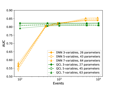
Figure 11: Average AUC values (calculated from the test samples) as a function of the training sample size up to $N_{\text{event}}^{\text{train}}=10,000$ for the new DNN and QCL models with $N_{\text{var}}=3$ (circles), 5 (squares) and 7 (triangles). The error bars represent the standard deviations of the average AUC values. The DNN points are slightly shifted horizontally from the nominal $N_{\text{event}}^{\text{train}}$ values to avoid overlapping.

5.4 CPU/memory usages for QCL implementation

The QCL algorithm runs on the Qulacs simulator with cloud Linux servers, as described in Sect. 3.2. Under this condition, we examine how the computational resources scale with the problem size. For the creation of input quantum states with $U_{\text{in}}(\boldsymbol{x})$, both CPU time and memory usage grow approximately linearly with $N_{\text{var}}$ or $N_{\text{event}}^{\text{train}}$. The creation of the variational quantum states with $U(\boldsymbol{\theta})$ shows an exponential increase in CPU time and memory usage with $N_{\text{var}}$ (i.e, number of qubits) up to $N_{\text{var}}=12$, roughly a factor 8 (4) increase in CPU time (memory) by incrementing the $N_{\text{var}}$ by one. The overall CPU time is by far dominated by the minimization process with COBYLA. It increases linearly with $N_{\text{event}}^{\text{train}}$ but grows exponentially with $N_{\text{var}}$, making it impractical to run the algorithm a sufficient number of times for $N_{\text{var}}\sim 10$ or more. The memory usage stays constant over $N_{\text{var}}$ during the COBYLA minimization process.

6 Conclusion

In this paper, we present studies of quantum machine learning for the event classification, commonly used as the application of conventional machine learning techniques to high-energy physics. The studies focus on the application of variational quantum algorithms using the implementations in QCL and VQC, and evaluate the performance in terms of AUC values of the ROC curves. The QCL performance is compared with the standard classical multi-variate classification techniques based on the BDT and DNN, and the VQC performance is tested using the simulator and real quantum computers. The overall QCL performance is comparable to the standard techniques if the problem is restricted to $N_{\text{var}}\leq 7$ and $N_{\text{event}}^{\text{train}}<\sim 10,000$. The QCL algorithm shows relatively flat AUC values in $N_{\text{event}}^{\text{train}}$, in contrast to the BDT and DNN algorithms, which show that the AUC values increase with increasing $N_{\text{event}}^{\text{train}}$ in the considered $N_{\text{event}}^{\text{train}}$ range. This characteristic QCL behavior could be considered as a possible advantage over the classical method at small $N_{\text{event}}^{\text{train}}$ where the DNN performance gets considerably worse if the number of trainable parameters of the DNN model is constrained to be similar to that of the QCL.

The VQC algorithm has been tested on quantum computers only for a small problem of $N_{\text{event}}^{\text{train}}=40$, but it shows that the algorithm does acquire the discrimination power. The VQC performances are similar on the simulator and real quantum computer within the measured accuracy. There is however an indication of increased errors due to hardware noise, that could prevent us from using an extended quantum circuit such as the SOE for the encoding of classical input data. The QCL and VQC algorithms show similar performance when they run on the simulators with the same conditions for the $N_{\text{var}}$ and $N_{\text{event}}^{\text{train}}$ values.

With a better control of the measurement and gate errors, it is expected that the performance of the variational quantum machine learning on quantum computers further improves, as demonstrated in Ref. Havlcek2019SupervisedLW with the SOE and increased depth of the variational circuit. Another potentially promising approach, proposed in Ref. Lloyd2020QuantumEF , is to train the encoding part of the variational algorithm to carry out a maximally separating embedding of classical input data into Hilbert space. This could provide a way to perform optimized measurements to distinguish different classes of data with a shallow quantum circuit, potentially reducing the impact from hardware errors on the variational part of the algorithm.

Conflict of interest

On behalf of all authors, the corresponding author states that there is no conflict of interest.

Code availability

The analysis code used in this study is available in https://github.com/kterashi/QML_HEP.

References

- (1) HEP ML Community: A Living Review of Machine Learning for Particle Physics. URL https://iml-wg.github.io/HEPML-LivingReview/
- (2) Apollinari, G., Béjar Alonso, I., Brüning, O., Fessia, P., Lamont, M., Rossi, L., Tavian, L.: High-Luminosity Large Hadron Collider (HL-LHC). CERN Yellow Rep. Monogr. 4, 1–516 (2017). DOI 10.23731/CYRM-2017-004
- (3) Evans, L., Bryant, P.: LHC Machine. JINST 3, S08001 (2008). DOI 10.1088/1748-0221/3/08/S08001
- (4) Mott, A., Job, J., Vlimant, J.R., Lidar, D., Spiropulu, M.: Solving a Higgs optimization problem with quantum annealing for machine learning. Nature 550(7676), 375–379 (2017). DOI 10.1038/nature24047
- (5) Zlokapa, A., Mott, A., Job, J., Vlimant, J.R., Lidar, D., Spiropulu, M.: Quantum adiabatic machine learning with zooming (2019)
- (6) Shapoval, I., Calafiura, P.: Quantum Associative Memory in HEP Track Pattern Recognition. EPJ Web Conf. 214, 01012 (2019). DOI 10.1051/epjconf/201921401012
- (7) Bapst, F., Bhimji, W., Calafiura, P., Gray, H., Lavrijsen, W., Linder, L.: A pattern recognition algorithm for quantum annealers. Comput. Softw. Big Sci. 4, 1 (2019). DOI 10.1007/s41781-019-0032-5
- (8) Zlokapa, A., Anand, A., Vlimant, J.R., Duarte, J.M., Job, J., Lidar, D., Spiropulu, M.: Charged Particle Tracking with Quantum Annealing-Inspired Optimization (2019)
- (9) Tüysüz, C., Carminati, F., Demirköz, B., Dobos, D., Fracas, F., Novotny, K., Potamianos, K., Vallecorsa, S., Vlimant, J.R.: Particle Track Reconstruction with Quantum Algorithms. p. 09013 (2020). DOI 10.1051/epjconf/202024509013
- (10) Das, S., Wildridge, A.J., Vaidya, S.B., Jung, A.: Track clustering with a quantum annealer for primary vertex reconstruction at hadron colliders (2019)
- (11) Wei, A.Y., Naik, P., Harrow, A.W., Thaler, J.: Quantum Algorithms for Jet Clustering. Phys. Rev. D 101(9), 094015 (2020). DOI 10.1103/PhysRevD.101.094015
- (12) Provasoli, D., Nachman, B., Bauer, C., de Jong, W.A.: A quantum algorithm to efficiently sample from interfering binary trees. Quantum Science and Technology 5(3), 035004 (2020). DOI 10.1088/2058-9565/ab8359
- (13) Bauer, C.W., De Jong, W.A., Nachman, B., Provasoli, D.: A quantum algorithm for high energy physics simulations (2019)
- (14) Cormier, K., Di Sipio, R., Wittek, P.: Unfolding measurement distributions via quantum annealing. JHEP 11, 128 (2019). DOI 10.1007/JHEP11(2019)128
- (15) Bauer, C.W., De Jong, W.A., Nachman, B., Urbanek, M.: Unfolding quantum computer readout noise. npj Quantum Inf. 6, 84 (2020). DOI 10.1038/s41534-020-00309-7
- (16) Preskill, J.: Quantum Computing in the NISQ era and beyond. Quantum 2, 79 (2018). DOI 10.22331/q-2018-08-06-79. URL https://doi.org/10.22331/q-2018-08-06-79
- (17) Johnson, M.W., Amin, M.H.S., Gildert, S., Lanting, T., Hamze, F., Dickson, N., Harris, R., Berkley, A.J., Johansson, J., Bunyk, P., Chapple, E.M., Enderud, C., Hilton, J.P., Karimi, K., Ladizinsky, E., Ladizinsky, N., Oh, T., Perminov, I., Rich, C., Thom, M.C., Tolkacheva, E., Truncik, C.J.S., Uchaikin, S., Wang, J., Wilson, B., Rose, G.: Quantum annealing with manufactured spins. Nature 473(7346), 194–198 (2011). DOI 10.1038/nature10012. URL http://dx.doi.org/10.1038/nature10012
- (18) Peruzzo, A., McClean, J., Shadbolt, P., Yung, M.H., Zhou, X.Q., Love, P., Aspuru-Guzik, A., O’Brien, J.: A variational eigenvalue solver on a photonic quantum processor. Nature Communications 5 (2014). DOI 10.1038/ncomms5213
- (19) Mitarai, K., Negoro, M., Kitagawa, M., Fujii, K.: Quantum circuit learning. Physical Review A 98(3) (2018). DOI 10.1103/physreva.98.032309. URL http://dx.doi.org/10.1103/PhysRevA.98.032309
- (20) Havlícek, V., Córcoles, A.D., Temme, K., Harrow, A.W., Kandala, A., Chow, J.M., Gambetta, J.M.: Supervised learning with quantum-enhanced feature spaces. Nature 567, 209–212 (2019). DOI 10.1038/s41586-019-0980-2
- (21) Pedregosa, F., Varoquaux, G., Gramfort, A., Michel, V., Thirion, B., Grisel, O., Blondel, M., Prettenhofer, P., Weiss, R., Dubourg, V., Vanderplas, J., Passos, A., Cournapeau, D., Brucher, M., Perrot, M., Duchesnay, E.: Scikit-learn: Machine learning in Python. Journal of Machine Learning Research 12, 2825–2830 (2011)
- (22) Speckmayer, P., Höcker, A., Stelzer, J., Voss, H.: The toolkit for multivariate data analysis, TMVA 4. Journal of Physics: Conference Series 219(3), 032057 (2010). DOI 10.1088/1742-6596/219/3/032057. URL https://doi.org/10.1088/1742-6596/219/3/032057
- (23) IBM Q Network. URL https://www.ibm.com/quantum-computing/network/overview/
- (24) Dua, D., Graff, C.: UCI machine learning repository (2017). URL http://archive.ics.uci.edu/ml
- (25) Baldi, P., Sadowski, P., Whiteson, D.: Searching for Exotic Particles in High-Energy Physics with Deep Learning. Nature Commun. 5, 4308 (2014). DOI 10.1038/ncomms5308
- (26) Qulacs. URL http://qulacs.org/index.html
- (27) Abraham, H., Akhalwaya, I.Y., Aleksandrowicz, G., Alexander, T., Alexandrowics, G., Arbel, E., Asfaw, A., Azaustre, C., AzizNgoueya, Barkoutsos, P., Barron, G., Bello, L., Ben-Haim, Y., Bevenius, D., Bishop, L.S., Bosch, S., Bucher, D., CZ, Cabrera, F., Calpin, P., Capelluto, L., Carballo, J., Carrascal, G., Chen, A., Chen, C.F., Chen, R., Chow, J.M., Claus, C., Clauss, C., Cross, A.J., Cross, A.W., Cross, S., Cruz-Benito, J., Cryoris, Culver, C., Córcoles-Gonzales, A.D., Dague, S., Dartiailh, M., DavideFrr, Davila, A.R., Ding, D., Drechsler, E., Drew, Dumitrescu, E., Dumon, K., Duran, I., Eastman, E., Eendebak, P., Egger, D., Everitt, M., Fernández, P.M., Fernández, P.M., Ferrera, A.H., Frisch, A., Fuhrer, A., GEORGE, M., GOULD, I., Gacon, J., Gadi, Gago, B.G., Gambetta, J.M., Garcia, L., Garion, S., Gawel-Kus, Gomez-Mosquera, J., de la Puente González, S., Greenberg, D., Grinko, D., Guan, W., Gunnels, J.A., Haide, I., Hamamura, I., Havlicek, V., Hellmers, J., Herok, Ł., Hillmich, S., Horii, H., Howington, C., Hu, S., Hu, W., Imai, H., Imamichi, T., Ishizaki, K., Iten, R., Itoko, T., Javadi-Abhari, A., Jessica, Johns, K., Kanazawa, N., Kang-Bae, Karazeev, A., Kassebaum, P., Knabberjoe, Kovyrshin, A., Krishnan, V., Krsulich, K., Kus, G., LaRose, R., Lambert, R., Latone, J., Lawrence, S., Liu, D., Liu, P., Mac, P.B.Z., Maeng, Y., Malyshev, A., Marecek, J., Marques, M., Mathews, D., Matsuo, A., McClure, D.T., McGarry, C., McKay, D., Meesala, S., Mezzacapo, A., Midha, R., Minev, Z., Mooring, M.D., Morales, R., Moran, N., Murali, P., Müggenburg, J., Nadlinger, D., Nannicini, G., Nation, P., Naveh, Y., Nick-Singstock, Niroula, P., Norlen, H., O’Riordan, L.J., Ogunbayo, O., Ollitrault, P., Oud, S., Padilha, D., Paik, H., Perriello, S., Phan, A., Pistoia, M., Pozas-iKerstjens, A., Prutyanov, V., Puzzuoli, D., Pérez, J., Quintiii, Raymond, R., Redondo, R.M.C., Reuter, M., Rodríguez, D.M., Ryu, M., SAPV, T., SamFerracin, Sandberg, M., Sathaye, N., Schmitt, B., Schnabel, C., Scholten, T.L., Schoute, E., Sertage, I.F., Shammah, N., Shi, Y., Silva, A., Siraichi, Y., Sitdikov, I., Sivarajah, S., Smolin, J.A., Soeken, M., Steenken, D., Stypulkoski, M., Takahashi, H., Taylor, C., Taylour, P., Thomas, S., Tillet, M., Tod, M., de la Torre, E., Trabing, K., Treinish, M., TrishaPe, Turner, W., Vaknin, Y., Valcarce, C.R., Varchon, F., Vogt-Lee, D., Vuillot, C., Weaver, J., Wieczorek, R., Wildstrom, J.A., Wille, R., Winston, E., Woehr, J.J., Woerner, S., Woo, R., Wood, C.J., Wood, R., Wood, S., Wootton, J., Yeralin, D., Yu, J., Zachow, C., Zdanski, L., Zoufalc, anedumla, azulehner, bcamorrison, brandhsn, chlorophyll zz, dime10, drholmie, elfrocampeador, faisaldebouni, fanizzamarco, gruu, kanejess, klinvill, kurarrr, lerongil, ma5x, merav aharoni, mrossinek, neupat, ordmoj, sethmerkel, strickroman, sumitpuri, tigerjack, toural, willhbang, yang.luh, yotamvakninibm: Qiskit: An open-source framework for quantum computing (2019). DOI 10.5281/zenodo.2562110
- (28) ibmq_johannesburg, IBM Quantum team. Retrieved from https://quantum-computing.ibm.com (2020). URL https://quantum-computing.ibm.com/docs/cloud/backends/systems/
- (29) ibmq_boeblingen, IBM Quantum team. Retrieved from https://quantum-computing.ibm.com (2020). URL https://quantum-computing.ibm.com/docs/cloud/backends/systems/
- (30) IBM Q system configuration maps. URL https://www.ibm.com/blogs/research/2019/09/quantum-computation-center/
- (31) Lloyd, S., Schuld, M., Ijaz, A., Izaac, J.A., Killoran, N.: Quantum embeddings for machine learning (2020)