CATCH: Characterizing and Tracking Colloids Holographically using deep neural networks

Abstract

In-line holographic microscopy provides an unparalleled wealth of information about the properties of colloidal dispersions. Analyzing one colloidal particle’s hologram with the Lorenz-Mie theory of light scattering yields the particle’s three-dimensional position with nanometer precision while simultaneously reporting its size and refractive index with part-per-thousand resolution. Analyzing a few thousand holograms in this way provides a comprehensive picture of the particles that make up a dispersion, even for complex multicomponent systems. All of this valuable information comes at the cost of three computationally expensive steps: (1) identifying and localizing features of interest within recorded holograms, (2) estimating each particle’s properties based on characteristics of the associated features, and finally (3) optimizing those estimates through pixel-by-pixel fits to a generative model. Here, we demonstrate an end-to-end implementation that is based entirely on machine-learning techniques. Characterizing and Tracking Colloids Holographically (CATCH) with deep convolutional neural networks is fast enough for real-time applications and otherwise outperforms conventional analytical algorithms, particularly for heterogeneous and crowded samples. We demonstrate this system’s capabilities with experiments on free-flowing and holographically trapped colloidal spheres.

I Introduction

Lorenz-Mie microscopy is a powerful technology for analyzing the properties of colloidal particles and measuring their three-dimensional motions Lee et al. (2007). Starting from in-line holographic microscopy images Sheng et al. (2006); Lee and Grier (2007), Lorenz-Mie microscopy measures the three-dimensional location, size and refractive index of each micrometer-scale particle in the microscope’s field of view. A typical measurement yields each particle’s position with nanometer precision over a hundred-micrometer range Cheong et al. (2010), its size with few-nanometer precision and its refractive index to within a part per thousand Krishnatreya et al. (2014). Results from sequences of holograms can be linked into trajectories for flow visualization Cheong et al. (2009), microrheology Cheong et al. (2008), photonic force microscopy Roichman et al. (2008), and to monitor transformations in colloidal dispersions’ properties Cheong et al. (2009); Shpaisman et al. (2012); Wang et al. (2015a, b). The availability of in situ data on particles’ sizes, compositions and concentrations is valuable for product development, process control and quality assurance in such areas as biopharmaceuticals Wang et al. (2016), semiconductor processing Cheong et al. (2017), and wastewater management Philips et al. (2017).

Unlocking the full potential of Lorenz-Mie microscopy requires an implementation that operates in real time and robustly interprets the non-ideal holograms that emerge from real-world samples. Here, we demonstrate that this challenge can be met with machine-learning techniques, specifically deep convolutional neural networks (CNNs) that are trained with synthetic data derived from physics-based models.

The analytical pipeline for Lorenz-Mie microscopy involves (1) identifying and localizing features of interest in recorded holograms and (2) estimating single-particle properties from the measured intensity pattern in each feature Lee et al. (2007); Soulez et al. (2007); Fung et al. (2011); Perry et al. (2012); Fung et al. (2012). The CATCH network performs these analytical steps over an exceptionally wide range of operating conditions, yielding results more robustly and $100$ times faster than the best reference implementations based on conventional algorithms Cheong et al. (2009); Krishnatreya and Grier (2014); Dimiduk et al. ; Hannel et al. (2018). The results are sufficiently accurate to solve real-world materials-characterization problems and can bootstrap nonlinear least-squares fits for the most demanding applications.

II Methods and Materials

II.1 Lorenz-Mie Microscopy

The custom-built holographic microscope used for Lorenz-Mie microscopy is shown schematically in Fig. 1(a). It illuminates the sample with a collimated laser beam whose electric field may be modeled as a plane wave of frequency $\omega$ and vacuum wavelength $\lambda$ propagating along the $\hat{z}$ axis,

$$\mathbf{E}_{0}(\mathbf{r})=u_{0}e^{ikz}e^{-i\omega t}\,\hat{x}.$$ (1)

Here, $u_{0}$ is the field’s amplitude and $k=2\pi n_{m}/\lambda$ is the wavenumber of light in a medium of refractive index $n_{m}$. The beam is assumed to be linearly polarized along $\hat{x}$. Our implementation uses a fiber-coupled diode laser (Coherent Cube) operating at $\lambda=$447\text{\,}\mathrm{nm}$$. The $10\text{\,}\mathrm{mW}$ beam is collimated at a diameter of $3\text{\,}\mathrm{mm}$, which more than fills the input pupil of the microscope’s objective lens (Nikon Plan Apo, $100\times$, numerical aperture 1.4, oil immersion). In combination with a $200\text{\,}\mathrm{mm}$ tube lens, this objective relays images to a grayscale camera (FLIR Flea3 USB 3.0) with a $1280\text{\times}1024\text{\,}\mathrm{p}\mathrm{i}\mathrm{x}\mathrm{e}\mathrm{l}$ sensor, yielding a system magnification of $48\text{\,}\mathrm{n}\mathrm{m}\mathrm{/}\mathrm{p}\mathrm{i}\mathrm{x}\mathrm{e}\mathrm{l}$.

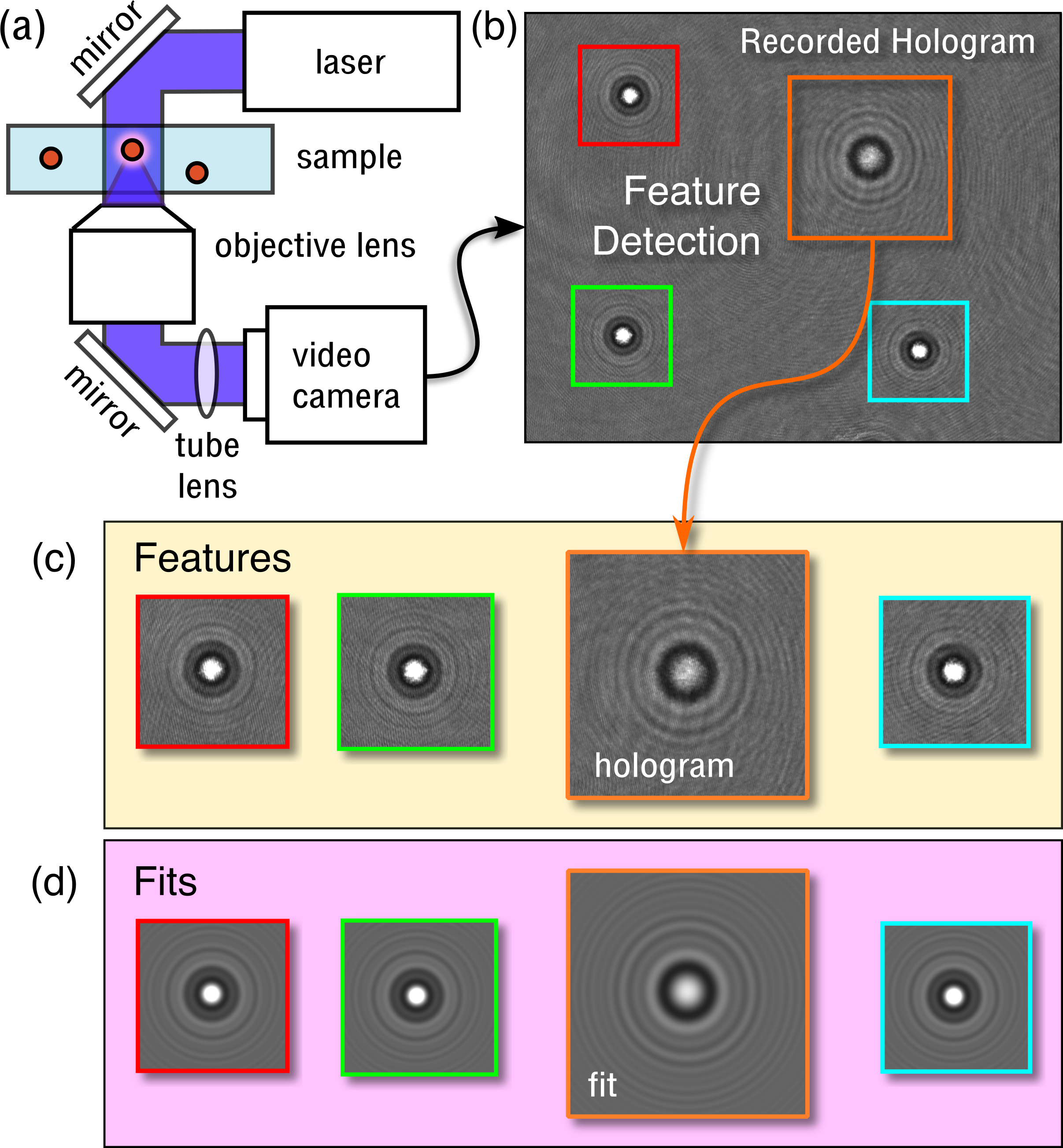
Figure 1: Schematic representation of Lorenz-Mie microscopy. (a) A fiber-coupled laser illuminates a colloidal sample. Light scattered by a particle interferes with the rest of the illumination in the focal plane of a microscope that magnifies and relays the interference pattern to a video camera. (b) Each recorded hologram is analyzed to detect features of interest. (c) Each feature is localized within a region whose size is dictated by the local signal-to-noise ratio. (d) Fitting a feature to the model in Eq. (3) yields estimates for $\mathbf{r}_{p}$, $a_{p}$ and $n_{p}$.

A colloidal particle located at $\mathbf{r}_{p}$ relative to the center of the microscope’s focal plane scatters a small proportion of the illumination to position $\mathbf{r}$ in the focal plane of the microscope,

$$\mathbf{E}_{s}(\mathbf{r})=E_{0}(\mathbf{r}_{p})\,\mathbf{f}_{s}(k(\mathbf{r}-\mathbf{r}_{p})).$$ (2)

The scattered wave’s relative amplitude, phase and polarization are described by the Lorenz-Mie scattering function, $\mathbf{f}_{s}(k\mathbf{r})$, which generally depends on the particle’s size, shape, orientation and composition Bohren and Huffman (1983); Mishchenko et al. (2001); Gouesbet and Gréhan (2011). For simplicity, we model the particle as an isotropic homogeneous sphere, so that $\mathbf{f}_{s}(k\mathbf{r})$ depends only on the particle’s radius, $a_{p}$, and its refractive index, $n_{p}$.

The incident and scattered waves interfere in the microscope’s focal plane. The resulting interference pattern is magnified by the microscope and is relayed to the camera Leahy et al. (2020), which records its intensity. Each snapshot in the camera’s video stream constitutes a hologram of the particles in the observation volume. The image in Fig. 1(b) is a typical experimentally recorded hologram of four colloidal silica spheres.

The distinguishing feature of Lorenz-Mie microscopy is the method used to extract information from recorded holograms. Rather than attempting to reconstruct the three-dimensional light field that created the hologram, Lorenz-Mie microscopy instead treats the analysis as an inverse problem, modeling the recorded intensity pattern as Lee et al. (2007)

$$I(\mathbf{r})=u_{0}^{2}\left|\hat{x}+e^{ikz_{p}}\mathbf{f}_{s}(k(\mathbf{r}-\mathbf{r}_{p}))\right|^{2}+I_{0},$$ (3)

where $I_{0}$ is the calibrated dark count of the camera. Fitting Eq. (3) to a measured hologram, such as the examples in Fig. 1(c), yields the ideal holograms shown in Fig. 1(d) together with values for each particle’s three-dimensional position, $\mathbf{r}_{p}$, as well as its radius, $a_{p}$, and its refractive index, $n_{p}$, at the imaging wavelength.

Lorenz-Mie microscopy also is implemented in a commercial holographic particle characterization instrument (Spheryx xSight), whose optical train differs significantly from that of the custom-built instrument and whose analytical software was developed independently. We use a combination of our own refined measurements and results obtained with xSight to provide experimental validatation for our machine-learning implementation.

II.1.1 Holographic optical trapping

Holographic optical traps with a vacuum wavelength of $1064\text{\,}\mathrm{nm}$ are projected into the sample using the same objective lens that is used for holographic microscopy. The traps are powered by a fiber laser (IPG Photonics YLR-10-LP) whose wavefronts are imprinted with computer-generated phase holograms Grier (2003) using a liquid crystal spatial light modulator (Holoeye Pluto). The modified beam is relayed into the objective lens with a dielectric multilayer dichroic mirror (Semrock), which permits simultaneous holographic trapping and holographic imaging.

II.2 Conventional Analysis

The first challenge in using Eq. (3) to analyze a hologram is to detect features of interest due to particles in the field of view. The concentric-ring pattern of a colloidal particle’s hologram can confound traditional object-detection algorithms that seek out simply connected regions of similar intensity. This problem has been addressed with two-dimensional mappings such as circular Hough transforms that coalesce concentric rings into compact peaks Cheong et al. (2009); Parthasarathy (2012); Krishnatreya and Grier (2014) that can be detected and localized with standard peak-finding algorithms Crocker and Grier (1996). This approach is reasonably effective for detecting and localizing holograms of well-separated particles. It performs poorly for concentrated samples, however, because overlapping scattering patterns create spurious peaks in the transformed image that can trigger false positive detections. These artifacts can be mitigated by limiting the range over which rings are coalesced at the cost of reducing sensitivity to larger holographic features. Optimizing the trade-off between false-positive and false-negative detections requires tuning the search range in parameter space and therefore creates a barrier to a fully-automated implementation.

Having selected regions of interest such as the examples in Fig. 1(c), the next step is to obtain estimates for the particles’ positions and properties that are good enough to bootstrap nonlinear least-squares fits. Reference implementations Dimiduk et al. ; Lee et al. (2007) of Lorenz-Mie microscopy use the initial localization estimate for the in-plane position and wavefront-curvature estimates for $a_{p}$ and $z_{p}$. The initial value of $n_{p}$ often is based on a priori knowledge, which is undesirable for unattended operation.

Ideally, these initial stages of analysis should proceed with minimal intervention, robustly identifying features and yielding reasonable estimates for parameters over the widest domain of possible values. Applications that would benefit from real-time performance also place a premium on fast algorithms, particularly those that perform effectively on standard computer hardware. These requirements can be satisfied with machine-learning algorithms, which surpass conventional algorithms in robustness, generality and speed.

II.3 Machine Learning Analysis

Previous efforts to streamline holographic particle characterization with machine-learning techniques Yevick et al. (2014); Hannel et al. (2018); Schneider et al. (2016), have addressed separate facets of the problem, specifically feature localization Hannel et al. (2018); Newby et al. (2018) and property estimation Yevick et al. (2014); Schneider et al. (2016). The former problem has been addressed with convolutional neural networks (CNNs), which are widely used for object localization Hannel et al. (2018); Redmon and Farhadi (2018). CNNs being far less common in regression applications, the latter problem has been addressed by feeding features’ radial intensity profiles into standard feed-forward neural networks Schneider et al. (2016) or support vector machines Yevick et al. (2014). Although each effort has been successful in its domain, combining them into an end-to-end analytical pipeline has provided only modest improvements in processing speed and robustness because of the overhead involved in extracting radial profiles and accounting for inevitable localization errors.

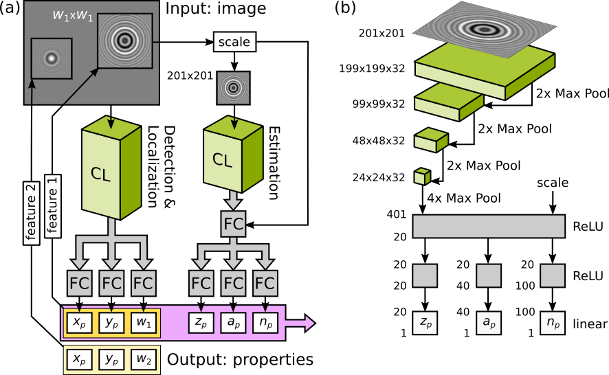
Figure 2: (a) CATCH uses a deep convolutional neural network (YOLOv3) to detect, localize and estimate the extent, $w_{n}$, of features in normalized holograms. Each feature is cropped from the image, scaled to a standard $201\text{\times}201\text{\,}\mathrm{p}\mathrm{i}\mathrm{x}\mathrm{e}\mathrm{l}$ format, and transferred to a second network that estimates the particle’s axial position, radius and refractive index. Each network consists of convolutional layers (CL) that analyze image data and feed their results into fully connected (FC) layers that perform regression. (b) Detailed view of the estimation network. Four convolutional layers alternate with max-pooling layers to map the input image into a $400$-element vector that is concatenated with the image’s scale factor. The resulting $401$-element vector is reduced to a $20$-element vector that describes the particle by a fully-connected layer with ReLU activation. The particle description is parsed into estimates for the axial position, $z_{p}$, particle radius, $a_{p}$, and refractive index, $n_{p}$, by three fully connected ReLU-activated layers feeding into three output layers with linear activation.

We address the need for fast, fully automated hologram analysis with a modular machine-learning system based entirely on highly optimized deep convolutional neural networks. The system, shown in Fig. 2, is trained with synthetic data that cover the entire anticipated domain of operating conditions without requiring manual annotation. Each module yields useful intermediate results, and the end-to-end system effectively bootstraps full-resolution fits, which we validate with experimental data.

The first module identifies features of interest in whole-field holograms, localizes them, and estimates their extents. Each detected feature then is cropped from the image and passed on to the second module, which estimates the particle’s radius, refractive index and axial position. A feature’s pixels and parameter estimates then can be passed on to the third module, not depicted in Fig. 2, which refines the parameter estimates by performing a nonlinear least-squares fit to Eq. (3). This modular architecture permits limiting the analysis to just what is required for the application at hand.

II.3.1 Detection and Localization

The detection module is based on the darknet implementation of YOLOv3, a state-of-the-art real-time object-detection framework that uses a convolutional neural network to identify features of interest in images, to localize them and, optionally, to classify them Redmon and Farhadi (2018). Given our focus on detection and localization, we adopt the comparatively simple and fast TinyYOLO variant, which consists of $23$ convolutional layers with a total of $25\,620$ adjustable parameters defining convolutional masks and their weighting factors.

Taking a grayscale image as input, the model returns estimates for each of the detected features’ in-plane positions, $(x_{p},y_{p})$, and their extents. These regions of interest can be used immediately to measure particle concentrations, for example, or they can be passed on to the next module for further analysis.

II.3.2 Parameter Estimation

CATCH estimates a particle’s axial position, $z_{p}$, radius, $a_{p}$, and refractive index, $n_{p}$, by passing the associated block of pixels through a second deep convolutional neural network for regression analysis. The regression network, depicted schematically in Fig. 2(b), consists of $19$ layers with a total of $34\,983$ trainable parameters and is constructed with the open-source Tensorflow framework Abadi et al. (2015) using the Keras application programming interface (API). The network’s input is a block of pixels cropped from the holographic image and then scaled down by an integer factor to $201\text{\times}201\text{\,}\mathrm{p}\mathrm{i}\mathrm{x}\mathrm{e}\mathrm{l}$. Scaling enables the estimator to accommodate scattering patterns with a wide range of extents in the camera plane.

The scaled image data initially pass through a series of convolutional and pooling layers that reduce the dimensionality of the regression space. The flattened output then is fed through a shared fully-connected layer along with the image’s scale factor to produce a $20$-element vector that describes the particle’s position in parameter space. This layer uses rectified linear activation units (ReLU) whose nonlinear response enables the network to learn complicated functions and whose near-linear form facilitates rapid training Glorot et al. (2011). The output of this layer is decoded by three independent ReLU-activated layers whose responses are scaled into dimensional values for $z_{p}$, $a_{p}$ and $n_{p}$ by linear output layers.

II.3.3 Training

Convolutional neural networks have the capacity to uncover low-dimensional approximate solutions to information-processing problems characterized by large numbers of internal degrees of freedom Rotskoff and Vanden-Eijnden (2018). To learn these patterns, however, the network must be trained with data that span the parameter range of interest at the desired resolution. Defining $R(p_{j})$ to be the range of the output parameter $p_{j}$ in a set of $M$ coupled parameters and $\Delta p_{j}$ to be the desired resolution in that parameter, naive scaling suggests that the number of elements required for a comprehensive training set should satisfy

$$N\leq\prod_{j=1}^{M}\frac{R(p_{j})}{\Delta p_{j}}.$$ (4)

The upper limit corresponds to sampling every possible solution, assuming that the generative function does not vary substantially over the range $\Delta p_{j}$. Smaller training sets suffice for problems that have an inherently lower-dimensional underlying structure. Because the two components of the CATCH network address different aspects of hologram analysis, we train them separately, thereby reducing the dimensionality of the overall problem and helping to ensure rapid and effective convergence with a reasonable amount of training.

We train the detection and localization network to recognize features in holographic microscopy images using a custom data set consisting of $N=$10\,000$$ synthetic holographic images for training and an additional $1000$ images for validation. If we assume that $x_{p}$ and $y_{p}$ are the only relevant output parameters, then this number of images should provide no worse than $\Delta x_{p}=\Delta y_{p}\approx$10\text{\,}\mathrm{p}\mathrm{i}\mathrm{x}\mathrm{e}\mathrm{l}$$ localization resolution for $1280\text{\times}1024\text{\,}\mathrm{p}\mathrm{i}\mathrm{x}\mathrm{e}\mathrm{l}$ images according to Eq. (4).

The synthetic images are designed to mimic experimental holograms over the anticipated domain of operation, with between zero and five particles positioned randomly in the field of view. Particles are assigned radii between $a_{p}=$200\text{\,}\mathrm{nm}$$ and $a_{p}=$5\text{\,}\mathrm{\SIUnitSymbolMicro m}$$ and refractive indexes between $n_{p}=$1.338$$ and $n_{p}=$2.5$$, and are located along the optical axis at distances from the focal plane between $z_{p}=$50\text{\,}\mathrm{p}\mathrm{i}\mathrm{x}\mathrm{e}\mathrm{l}\mathrm{s}$$ and $z_{p}=$600\text{\,}\mathrm{p}\mathrm{i}\mathrm{x}\mathrm{e}\mathrm{l}\mathrm{s}$$, with each axial pixel corresponding to the in-plane scale of $48\text{\,}\mathrm{nm}$. The extent, $w_{p}$, of each holographic feature is defined to be the diameter enclosing $20$ interference fringes and therefore scales with the particle’s size and axial position. Ideal holograms computed with Eq. (3) are degraded with $5\text{\,}\mathrm{\char 37\relax}$ additive Gaussian noise. The ground truth for localization training consists of the in-plane coordinates, $(x_{p},y_{p})$, of each feature in a hologram together with the features’ extents, $w_{p}$. We trained for $500\,000\text{\,}\mathrm{e}\mathrm{p}\mathrm{o}\mathrm{c}\mathrm{h}\mathrm{s}$ with a batch size of $64$ images and $32$ subdivisions.

We train the estimator network on a second set of $N=$10\,000$$ synthetic single-particle holograms with a validation set of $1000$ images, covering the same parameter range used to train the localization network. In addition to adding $5\text{\,}\mathrm{\char 37\relax}$ Gaussian noise to the intensity pattern, we also incorporate up to $10\text{\,}\mathrm{p}\mathrm{i}\mathrm{x}\mathrm{e}\mathrm{l}$ localization error and $10\text{\,}\mathrm{\char 37\relax}$ error in extent to simulate worst-case performance by the first stage of analysis. The network is trained with the Adam optimizer Kingma and Ba (2014) for $5000$ epochs with a batch size of $64$ images using minimal dropout and L2 regularization to prevent overfitting. Naive application of Eq. (4) then suggests that we should expect $\Delta z_{p}\leq$1.2\text{\,}\mathrm{\SIUnitSymbolMicro m}$$, $\Delta a_{p}\leq$0.22\text{\,}\mathrm{\SIUnitSymbolMicro m}$$ and $\Delta n_{p}\leq$0.05$$.

III Results and Discussion

III.1 Validation with Synthetic Data

The CATCH network’s performance is validated first with synthetic data and then through experiments on model systems. The synthetic validation data set consists of $10\,000$ holograms that were generated independently of the data used for training. This data set is designed to assess performance under ideal imaging conditions without the additional complexity of overlapping features in multi-particle holograms. Each synthetic hologram contains one particle with randomly selected properties placed at random in the $1280\text{\times}1024\text{\,}\mathrm{p}\mathrm{i}\mathrm{x}\mathrm{e}\mathrm{l}$ field of view and includes $5\text{\,}\mathrm{\char 37\relax}$ additive Gaussian noise.

III.1.1 Processing Speed

Tests were performed with hardware-accelerated versions of each algorithm running on a desktop workstation equipped with an NVIDIA Titan Xp GPU. On this hardware, conventional algorithms Cheong et al. (2009); Krishnatreya and Grier (2014); Crocker and Grier (1996); Allan et al. (2016); Dimiduk et al. perform a complete end-to-end single-frame analysis in roughly $1\text{\,}\mathrm{s}$. By contrast, the CATCH network’s detector and localizer requires $20\text{\,}\mathrm{ms}$ per frame and the machine-learning estimator requires an additional $0.9\text{\,}\mathrm{ms}$ per feature. This is fast enough for real-time performance assuming a typical frame rate of $30\text{\,}\mathrm{f}\mathrm{r}\mathrm{a}\mathrm{m}\mathrm{e}\mathrm{s}\mathrm{/}\mathrm{s}$.

III.1.2 Detection Accuracy

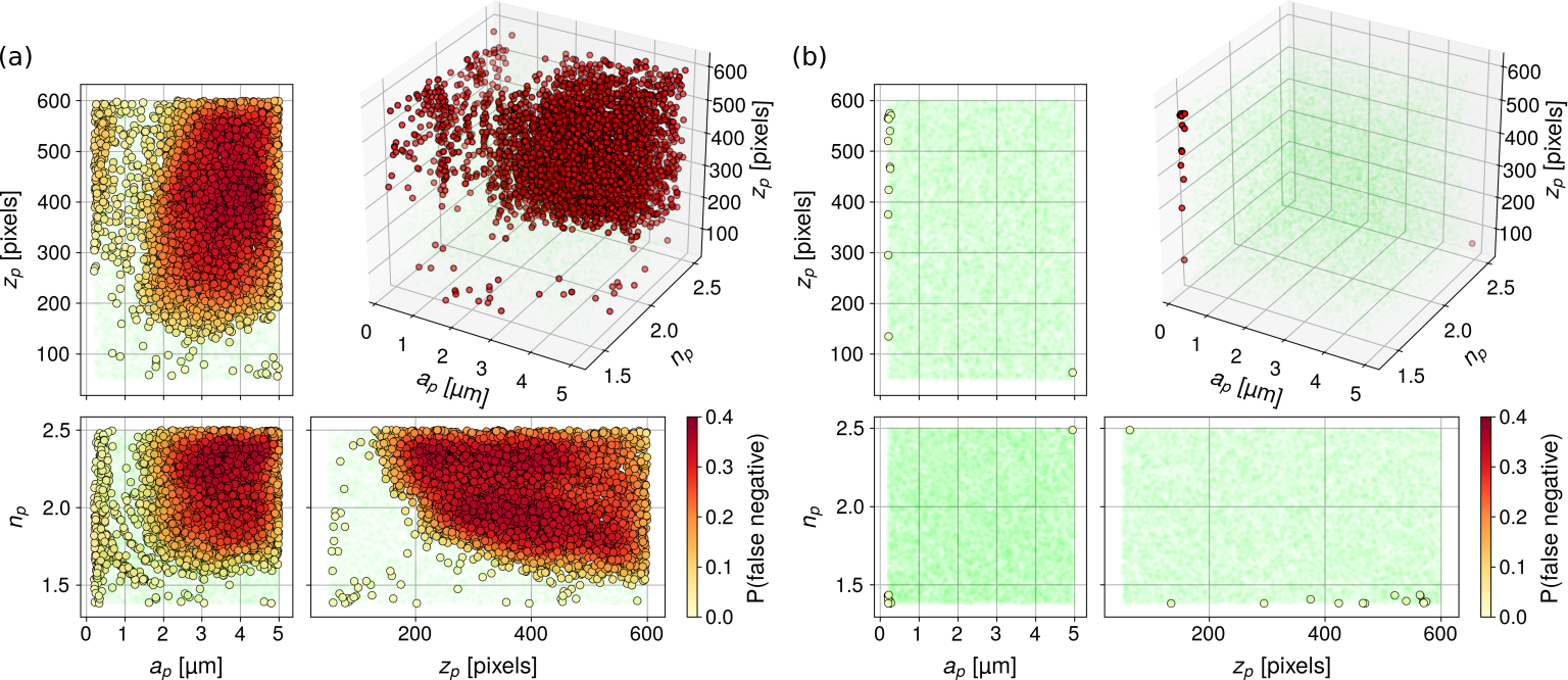
Figure 3: False negative detections in simulated holograms plotted as filled circles and colored by the local error probability. (Green) points denote correct positive detections. (a) Conventional feature detection algorithms miss up to $40\text{\,}\mathrm{\char 37\relax}$ of particles in $10\,000$ simulated single-particle holograms. (b) The convolutional neural network misses fewer than $0.1\text{\,}\mathrm{\char 37\relax}$ of the $25\,000\text{\,}\mathrm{p}$lotted features over the same parameter range.

When assessing detection accuracy, we are concerned primarily with the rate of false negative detections. False positive detections are less concerning because they can be identified and filtered through post-processing, but false negatives represent lost information. Conventional feature detection algorithms Cheong et al. (2009); Parthasarathy (2012); Krishnatreya and Grier (2014) have been shown to work well for small, weakly-scattering particles. Over the larger range of parameter space plotted in Fig. 3(a), however, conventional algorithms fail to detect up to $40\text{\,}\mathrm{\char 37\relax}$ of particles, even under ideal conditions. Over the same range, the neural network misses fewer than $0.1\text{\,}\mathrm{\char 37\relax}$ of features, as shown in Fig. 3(b), and proposes no false positives. The false negatives occur for very small particles that are nearly index matched to the medium whose holograms have the poorest signal-to-noise ratios in this study.

This dramatic improvement in detection reliability greatly expands the parameter space for unattended Lorenz-Mie particle characterization. It allows for automated analysis of larger volumes, larger particles and larger ranges of particle characteristics in a single sample. Such systems could have been analyzed previously, but would have required human intervention.

III.1.3 Localization and Feature Extent

Localization accuracy is assessed for true-positive detections on synthetic images using the input particle locations as the ground truth. As presented in Fig. 4, the net in-plane localization error is smaller than $\Delta x_{p}=\Delta y_{p}=$1.5\text{\,}\mathrm{p}\mathrm{i}\mathrm{x}\mathrm{e}\mathrm{l}$$, or $70\text{\,}\mathrm{nm}$, across the entire range of parameters, and typically is better than $1\text{\,}\mathrm{p}\mathrm{i}\mathrm{x}\mathrm{e}\mathrm{l}$. The localizer therefore outperforms the naive estimate for localization precision in Eq. (4), presumably because the CNN has identified a low-dimensional representation for the problem. Estimates for the features’ extents, $w_{p}$, vary from the ground truth by $15\text{\,}\mathrm{\char 37\relax}$ with a bias toward underprediction. This figure of merit is a target for future improvement because scaling errors propagate into the regression analysis and are found to increase errors in the estimates for $a_{p}$ and $z_{p}$.

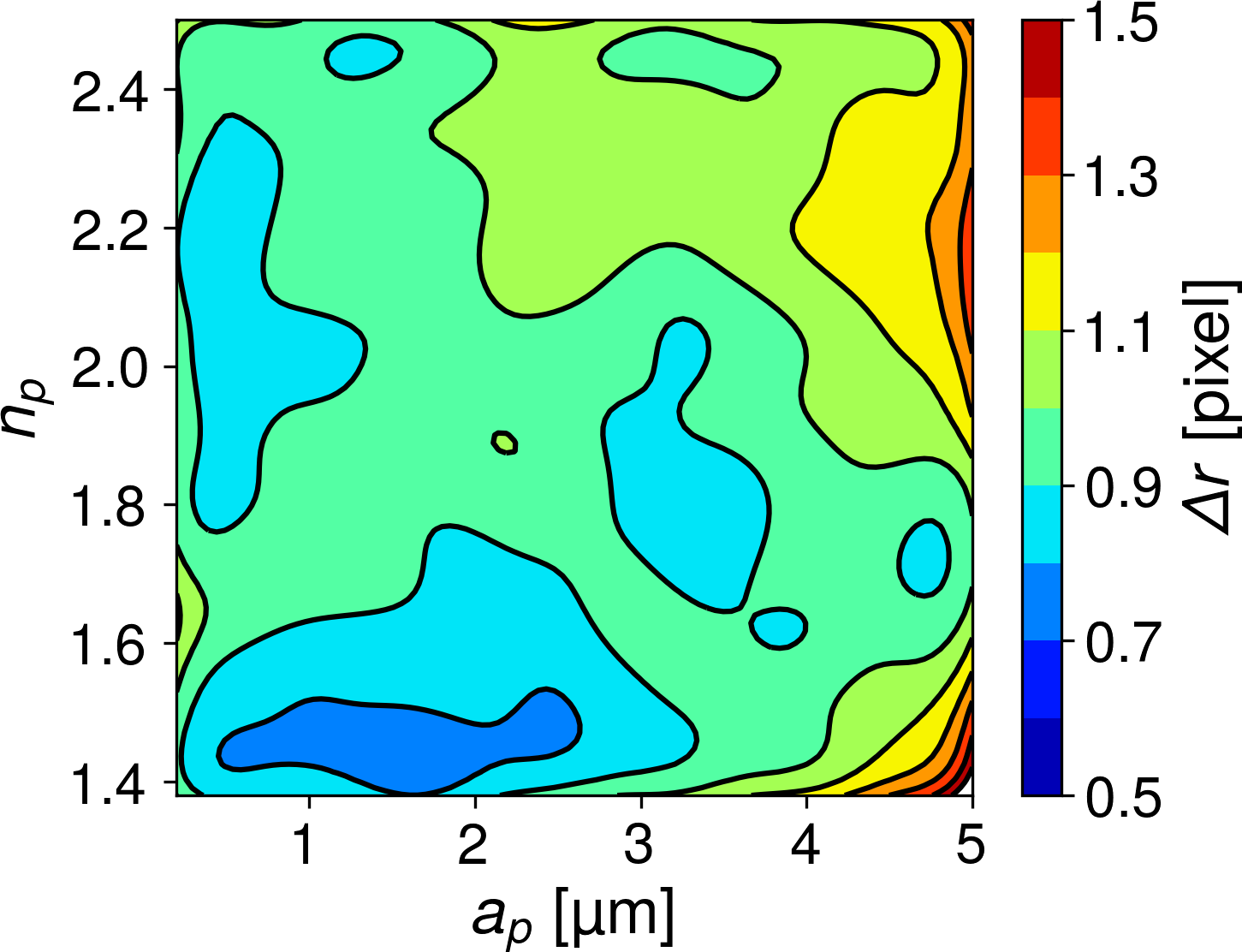
Figure 4: In-plane localization error, $\Delta r$, as a function of particle radius and refractive index, averaged over axial position, for all $24\,994$ true positive detections. Obtained from TinyYOLO implementation of the network localizer.

III.1.4 Characterization

Figure 5 summarizes the regression network’s performance for estimating axial position, particle size and refractive index in the validation set of synthetic data. Each panel shows the root-mean-square error for one parameter as a function of $a_{p}$ and $n_{p}$, averaged over $\mathbf{r}_{p}$. Over most of the parameter domain, the estimator predicts the relevant parameter to within $10\text{\,}\mathrm{\char 37\relax}$. This is not quite as good as the naive estimate from Eq. (4) proposes, which suggests that the parameter space has not been sampled finely enough to resolve the structure of the underlying Lorenz-Mie scattering problem. Achieving the part-per-thousand precision offered by nonlinear least-squares fits would require on the order of $N=${10}^{9}$$ images, according to naive scaling.

Conventional gradient-descent fits to the Lorenz-Mie theory display pronounced anticorrelations between $a_{p}$ and $n_{p}$ Ruffner et al. (2018). No strong cross-parameter correlation is evident in the error surfaces plotted in Fig. 5. This difference highlights a potential benefit of machine-learning regression for complex image-analysis tasks. Unlike conventional fitters, machine-learning algorithms do not attempt to follow smooth paths through complex error landscapes, but rather rely upon an internal representation of the error landscape that is built up during training. Directly reading out an optimal solution from such an internal representation is computationally efficient and less prone to trapping in local minima of the conventional error surface. Most importantly, unsupervised parameter estimation eliminates the need for a priori information or human intervention in colloidal materials characterization.

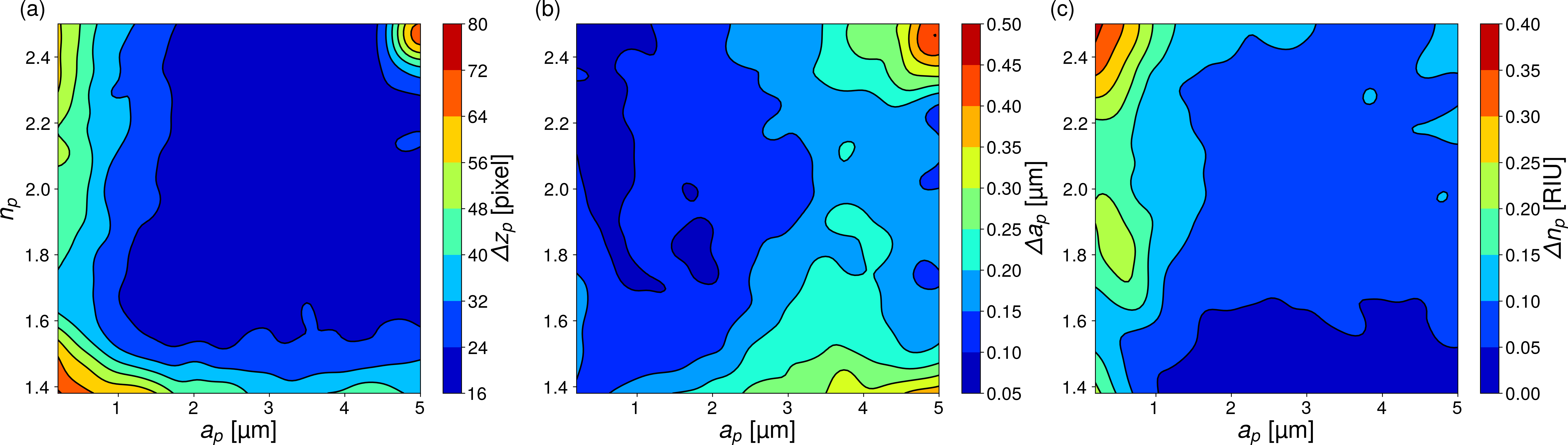
Figure 5: Root-mean-square errors in (a) axial position, $\Delta z_{p}$, (b) radius, $\Delta a_{p}$ and (c) refractive index, $\Delta n_{p}$, as a function of radius and refractive index on a set of $25\,000$ cropped holograms. Results are averaged over placement errors.

III.2 Validation with Experimental Data

Having validated the CATCH system’s performance with synthetic data, we use it to analyze experimental data. Some applications, such as measuring particle concentations, can be undertaken with the detection and localization module alone. Some other tasks require characterization data and can be performed with the output of the estimation module. Still others use machine-learning estimates to bootstrap nonlinear least-squares fits to Eq. (3). The full end-to-end mode of operation benefits from the speed and robustness of machine-learning estimation and delivers the precision of nonlinear optimization Lee et al. (2007); Krishnatreya et al. (2014).

III.2.1 Fast and accurate colloidal concentration measurements

CATCH’s detection subsystem rapidly counts particles passing through the microscope’s observation volume and thus can measure their concentration. Its ability to detect particles over a large axial range is an advantage relative to conventional image-based particle-counting techniques Ripple and Hu (2016), which have a limited depth of focus and thus a more restricted observation volume.

Although the holographic microscope’s measurement volume might be known a priori, CATCH also can estimate the effective observation volume from the least bounding rectangular prism that encloses all detected particle locations. This internal calibration is most effective for particles that remain dispersed throughout the height of the channel. For such samples, this protocol addresses uncertainties due to variations in actual channel dimensions and accounts for detection limits near the boundaries of the observation volume.

We demonstrate machine-learning concentration measurements on a heterogeneous sample created by mixing four different populations of monodisperse colloidal spheres: two sizes of polystyrene spheres (Thermo Scientific, catalog no. 5153A, $a_{p}=$0.79\text{\,}\mathrm{\SIUnitSymbolMicro m}$$; Duke Standards, catalog no. 4025A, $a_{p}=$1.25\text{\,}\mathrm{\SIUnitSymbolMicro m}$$), and two sizes of silica spheres (Duke Standards, catalog no. 8150, $a_{p}=$0.79\text{\,}\mathrm{\SIUnitSymbolMicro m}$$; Bangs Laboratories, catalog no. SS05N, $a_{p}=$1.15\text{\,}\mathrm{\SIUnitSymbolMicro m}$$). Each population of spheres is dispersed in water at a nominal concentration of $4\text{\times}{10}^{6}\text{\,}\mathrm{p}\mathrm{a}\mathrm{r}\mathrm{t}\mathrm{i}\mathrm{c}\mathrm{l}\mathrm{e}\mathrm{s}\mathrm{/}\mathrm{m}\mathrm{L}$. Equal volumes of these monodisperse stock dispersions are mixed to create the heterogeneous sample. Such mixtures can pose challenges for conventional techniques such as dynamic light scattering, which assume that the scatterers are drawn from a unimodal distribution. No other particle-characterization technique would be able to differentiate particles with similar sizes but different compositions.

A $30\text{\,}\mathrm{\SIUnitSymbolMicro L}$ aliquot of the four-component dispersion is introduced into a channel formed by bonding the edges of a #1.5 cover glass to the face of a glass microscope slide with UV-cured adhesive (Norland Products, catalog no. NOA81). The resulting channel is roughly $1\text{\,}\mathrm{mm}$ wide, $2\text{\,}\mathrm{cm}$ long and $15\text{\,}\mathrm{\SIUnitSymbolMicro m}$ deep. Once the cell is mounted on the stage of the holographic microscope, we transport roughly $10\text{\,}\mathrm{\SIUnitSymbolMicro L}$ of this sample through the microscope’s observation volume at roughly $1\text{\,}\mathrm{mm}\text{\,}{\mathrm{s}}^{-1}$ in a capillary-driven flow. A data set of $47\,539$ video frames recorded over $26\text{\,}\mathrm{min}$ probes a total volume of $0.83\pm 0.14\text{\,}\mathrm{\SIUnitSymbolMicro L}$ given the effective observation volume of $25\text{\times}38\text{\times}(18\pm 3.)\text{\,}\mathrm{\SIUnitSymbolMicro m}$, or $17\pm 3.\text{\,}\mathrm{pL}$. The $18\text{\,}\mathrm{\char 37\relax}$ uncertainty in the axial extent dominates the uncertainty in the effective observation volume. In-plane dimensions are determined to better than $1\text{\,}\mathrm{\char 37\relax}$.

The CATCH detection module reports $2967$ features in this sample, which corresponds to a net concentration of $(3.6\pm 0.6)\text{\times}{10}^{6}\text{\,}\mathrm{p}\mathrm{a}\mathrm{r}\mathrm{t}\mathrm{i}\mathrm{c}\mathrm{l}\mathrm{e}\mathrm{s}\mathrm{/}\mathrm{m}\mathrm{L}$. This value is consistent with expectations based on the concentrations of the stock dispersions and agrees reasonably well with the value of of $3.1\text{\times}{10}^{6}\text{\,}\mathrm{p}\mathrm{a}\mathrm{r}\mathrm{t}\mathrm{i}\mathrm{c}\mathrm{l}\mathrm{e}\mathrm{s}\mathrm{/}\mathrm{m}\mathrm{L}$ obtained with xSight. CATCH is fast enough to complete the concentration estimate in the time required to record the images.

III.2.2 Characterizing heterogeneous dispersions

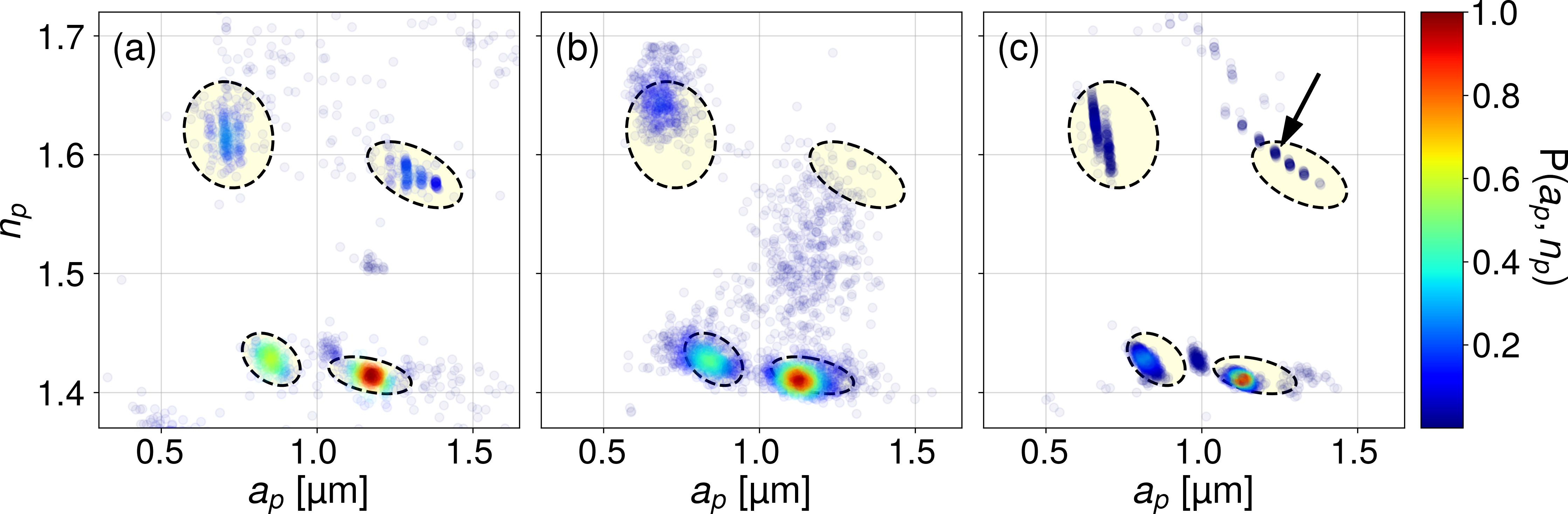
Figure 6: Measurements of the radius, $a_{p}$, and refractive index, $n_{p}$, of a mixture of four monodisperse populations of polystyrene and silica spheres. Each point represents the properties of a single particle and is colored by the relative probability density of observations, $P(a_{p},n_{p})$. (a) Properties of $1917$ particles reported by xSight. Ellipses represent $99\text{\,}\mathrm{\char 37\relax}$ confidence intervals for each population of particles. (b) Predictions for another $2967$ particles recorded on the custom-built microscope and analyzed by the CATCH convolutional neural network. (c) CATCH predictions refined by nonlinear least-squares fits to Eq. (3). The arrow indicates the globally optimal characterization parameters for the large polystyrene spheres in this system.

The detection subsystem is not trained to distinguish among different types of particles. The estimation subsystem, however, can differentiate particles both by size and also by refractive index. The scatter plots in Fig. 6 show holographic particle characterization data of thousands of particles from the four-component dispersion described in the previous section. Points are colored by the relative density of observations, $P(a_{p},n_{p})$.

The results plotted in Fig. 6(a) are obtained with xSight and will be treated as the ground truth. Dashed ellipses superimposed on the particle-resolved characterization data represent $99\text{\,}\mathrm{\char 37\relax}$ confidence intervals obtained with principal component analysis for each of the four populations of particles. Additional data points outside these regions correspond to impurity particles such as dimers as well as a small number of spurious results caused by overlapping holograms. The same ellipses are superimposed on the results obtained with CATCH in Fig. 6(b) and on the refined estimates bootstrapped by CATCH in Fig. 6(c).

The upper two ellipses centered on refractive index around $1.60$ correspond to the two sizes of polystyrene spheres in the mixture. The two lower ellipses correspond to the silica spheres with a refractive index around $1.40$. xSight clearly distinguishes the two compositions of spheres by their refractive indexes. The ability to differentiate particle populations both by size and by composition is a unique advantage of holographic particle characterization relative to all other particle characterization technologies.

Figure 6(b) shows results from a separate measurement on the same colloidal sample performed with the custom-built holographic video microscope and analyzed with CATCH. All four populations are visible in the scatter plot, and the silica characterization results agree quantitatively with xSight measurements. The larger polystyrene spheres appear as a poorly localized cloud of points because that range of parameter space is characterized by a large number of nearly degenerate solutions Ruffner et al. (2018).

Although CATCH does not achieve the full precision of the Lorenz-Mie analysis, its results still are close enough to the ground truth to bootstrap nonlinear least-squares fits. The results in Fig. 6(c) show the same data from Fig. 6(b) after nonlinear fitting. The predictions for all four populations are consistent with xSight measurements, albeit with systematic offsets that likely arise from differences in the two instruments’ optical trains that are not accounted for by the model in Eq. (3) Leahy et al. (2020). The root-mean-squared displacements of the CATCH estimates from the corresponding refined values, $\Delta a_{p}=$89\text{\,}\mathrm{nm}$$ and $\Delta n_{p}=$0.04$$, are consistent with the errors estimated with synthetic validation data in Sec. III.1.

Results for the larger polystyrene spheres do not converge into a well-defined cluster, but rather form a series of islands that constitute a set of nearly degenerate solutions Ruffner et al. (2018). The same structure also can be discerned in xSight results. The central island, indicated by an arrow in Fig. 6(c), appears to correspond to the globally optimal solution based on the chi-squared statistic for all fits. Neither the Levenberg-Marquardt least-squares optimizer nor the Nelder-Mead simplectic search algorithm consistently converges to this particular solution starting from the CATCH estimates for these particles. Even for this challenging case, however, the parameters proposed by CATCH converge to reasonable values within the expected confidence interval, which demonstrates that they are good enough for practical applications.

III.2.3 Tracking confined sedimentation

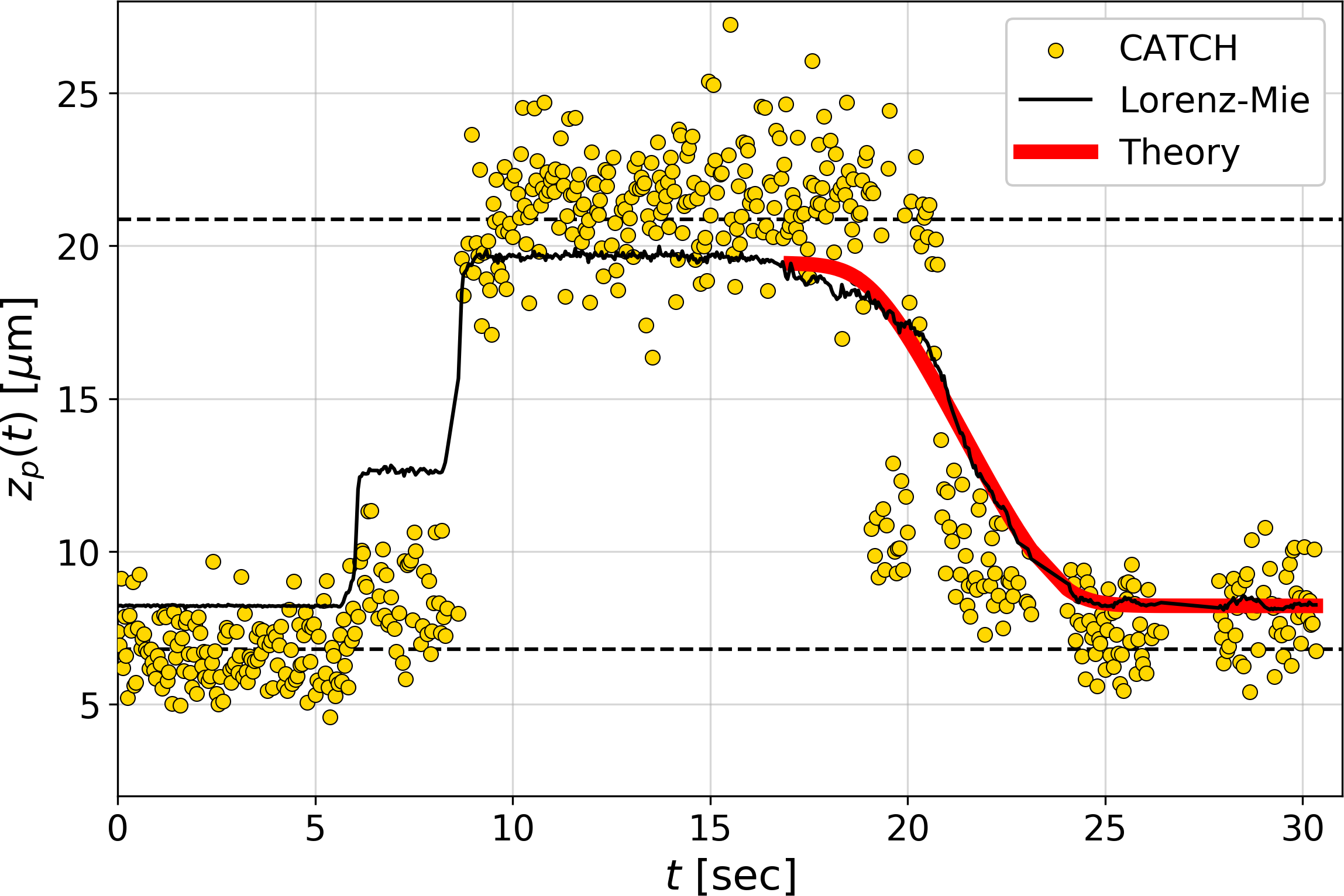
Figure 7: Estimated (points) and refined (solid black curve) axial trajectory of a colloidal silica sphere being lifted to the upper wall of a water-filled channel and allowed to sediment to the lower wall under gravity. The heavy (red) curve is a fit to Eq. (5) for the density of the particle and the positions of the walls, which are indicated by horizontal dashed lines.

To illustrate three-dimensional particle tracking based on CATCH estimation, we measure the sedimentation of a colloidal sphere between two parallel horizontal surfaces. The influence of slot confinement on a colloidal sphere’s in-plane drag coefficient has been reported previously using conventional imaging Dufresne et al. (2001). The axial drag coefficient has not been reported, presumably because of the difficulty of measuring the axial position with sufficient accuracy.

We perform the measurement on a colloidal silica sphere (Bangs Laboratories, catalog no. SS05N) dispersed in $30\text{\,}\mathrm{\SIUnitSymbolMicro L}$ of deionized water that is contained in a glass sample chamber formed by bonding the edges of a glass cover slip to the face of a glass microscope slide. Holographic optical traps are projected into the sample using the same objective lens that is used to record holograms Grier (2003). We lift the sphere to the top of its sample chamber using a holographic optical trap Grier (2003); O’Brien and Grier (2019) and then release it. Analyzing the particle’s trajectory then yields an estimate for the buoyant mass density that can be compared with an orthogonal estimate based on the particle’s holographically measured size and refractive index.

The discrete data points in Fig. 7 are machine-learning estimates of the particle’s axial position, $z_{p}(t)$, as a function of time, recorded at $24\text{\,}\mathrm{f}\mathrm{r}\mathrm{a}\mathrm{m}\mathrm{e}\mathrm{s}\mathrm{/}\mathrm{s}$. The solid (black) curve is obtained by fitting the sphere’s hologram to Eq. (3) starting from machine-learning estimates for $\mathbf{r}_{p}(t)$, $a_{p}$ and $n_{p}$. These fits converge to $a_{p}=$1.14\pm 0.04\text{\,}\mathrm{\SIUnitSymbolMicro m}$$ and $n_{p}=$1.398\pm 0.005$$, which are consistent with the manufacturer’s specification and with the population-averaged properties, $a_{p}=$1.17\pm 0.15\text{\,}\mathrm{\SIUnitSymbolMicro m}$$ and $n_{p}=$1.42\pm 0.02$$, obtained with xSight. The root-mean-square axial tracking error for this data set is $\Delta z_{p}=$2.8\text{\,}\mathrm{\SIUnitSymbolMicro m}$$, which is consistent with errors estimated in Sec. III.1.

In addition to being acted upon by gravity, the particle also is hydrodynamically coupled to the walls of its sample chamber, which reduces its mobility. The particle sediments under gravity at a rate,

$$\frac{dz_{p}}{dt}=-\frac{4}{3}\pi a_{p}^{3}\,(\rho_{p}-\rho_{m})\,g\,\mu(z_{p}),$$ (5a)

that depends on the difference between its mass density, $$\rho_{p} \rho_{m} \mu(z_{p}) z=z_{0} z=z_{0}+H$$, and the mass density of the medium, . Hydrodynamic coupling to the parallel glass walls reduces the sphere’s mobility, , by an amount that depends on its axial position within the channel. Specifically, the flow field due to the sedimenting sphere is modified by no-slip boundary conditions at the lower and upper walls, which are located at and relative to the microscope’s focal plane, respectively. For simplicity, we model the resulting dependence by combining lowest-order single-wall corrections Happel and Brenner (1991) with the Oseen linear superposition approximation to obtain

$$\mu(z)\approx\frac{1}{6\pi\eta a_{p}}\left(1-\frac{9}{8}\frac{a_{p}}{z-z_{0}}-\frac{9}{8}\frac{a_{p}}{H-z+z_{0}}\right),$$ (5b)

where $\eta=$0.89\text{\,}\mathrm{mPa}\text{\,}\mathrm{s}$$ is the viscosity of water. The solid (red) curve in Fig. 7 is a fit of the refined data (black curve) to the prediction of Eq. (5) with $z_{0}$, $H$ and $\rho_{p}$ as adjustable parameters. This fit yields $\rho_{p}=$2.18\begin{subarray}{c}+0.07\\ -0.20\end{subarray}\text{\,}\mathrm{g}\text{\,}{\mathrm{cm}}^{-3}$$ assuming $\rho_{m}=$0.997\text{\,}\mathrm{g}\text{\,}{\mathrm{cm}}^{-3}$$ for water.

The particle’s comparatively low mass density is consistent with its low refractive index. Maxwell Garnett effective medium theory Markel (2016) suggests that the particle’s density may be estimated from its refractive index as

$$\rho_{p}=\rho_{0}\frac{L_{m}(n_{p})-L_{m}(1)}{L_{m}(n_{0})-L_{m}(1)},$$ (6)

where $\rho_{0}=$2.20\text{\,}\mathrm{g}\text{\,}{\mathrm{cm}}^{-3}$$ is the density of fused silica, $n_{0}=$1.465$$ is the refractive index of fused silica at the imaging wavelength, and

$$L_{m}(n)=\frac{n^{2}-n_{m}^{2}}{n^{2}+2n_{m}^{2}}$$ (7)

is the Lorentz-Lorenz function. The result, $\rho_{p}=$1.90\pm 0.10\text{\,}\mathrm{g}\text{\,}{\mathrm{cm}}^{-3}$$, is consistent with the lower bound of the kinematic estimate, and so helps to validate Krishnatreya et al. (2014) the accuracy and precision with which CATCH characterizes and tracks colloidal particles.

IV Conclusions

CATCH is an end-to-end machine-learning system for analyzing the properties of colloidal dispersions from holographic microscopy images. Based on YOLO and a custom-designed deep convolutional neural network, this system delivers the full characterization and tracking power of Lorenz-Mie microscopy with greatly improved speed and robustness. This implementation has been validated both with simulated data and also through experimental measurements on model colloidal dispersions. These measurements illustrate the utility of CATCH for measuring the concentrations of colloidal dispersions, for characterizing the particles in heterogeneous dispersions, and for measuring single-particle dynamics.

More generally, CATCH embodies a paradigm shift in measurement theory, with machine-learning algorithms replacing physical mechanisms and physics-based models in precision measurements. The availability of such “brain-in-a-box” instruments increases the speed and robustness of such measurements and also promises access to physical phenomena that cannot readily be measured by other means.

Our open-source implementation of the end-to-end CATCH system is available online at https://github.com/laltman2/CNNLorenzMie.

References

- Lee et al. (2007) Sang-Hyuk Lee, Yohai Roichman, Gi-Ra Yi, Shin-Hyun Kim, Seung-Man Yang, Alfons van Blaaderen, Peter van Oostrum, and David G. Grier, “Characterizing and tracking single colloidal particles with video holographic microscopy,” Opt. Express 15, 18275–18282 (2007).
- Sheng et al. (2006) Jian Sheng, Edwin Malkiel, and Joseph Katz, “Digital holographic microscope for measuring three-dimensional particle distributions and motions,” Appl. Opt. 45, 3893–3901 (2006).
- Lee and Grier (2007) Sang-Hyuk Lee and David G Grier, “Holographic microscopy of holographically trapped three-dimensional structures,” Opt. Express 15, 1505–1512 (2007).
- Cheong et al. (2010) Fook Chiong Cheong, Bhaskar Jyoti Krishnatreya, and David G. Grier, “Strategies for three-dimensional particle tracking with holographic video microscopy,” Opt. Express 18, 13563–13573 (2010).
- Krishnatreya et al. (2014) Bhaskar Jyoti Krishnatreya, Arielle Colen-Landy, Paige Hasebe, Breanna A. Bell, Jasmine R. Jones, Anderson Sunda-Meya, and David G. Grier, “Measuring Boltzmann’s constant through holographic video microscopy of a single sphere,” Am. J. Phys. 82, 23–31 (2014).
- Cheong et al. (2009) Fook Chiong Cheong, Bo Sun, Rémi Dreyfus, Jesse Amato-Grill, Ke Xiao, Lisa Dixon, and David G. Grier, “Flow visualization and flow cytometry with holographic video microscopy,” Opt. Express 17, 13071–13079 (2009).
- Cheong et al. (2008) Fook Chiong Cheong, Simone Duarte, Sang-Hyuk Lee, and David G. Grier, “Holographic microrheology of polysaccharides from Streptococcus mutans biofilms,” Rheol. Acta 48, 109–115 (2008).
- Roichman et al. (2008) Yohai Roichman, Bo Sun, Allan Stolarski, and David G. Grier, “Influence of non-conservative optical forces on the dynamics of optically trapped colloidal spheres: The fountain of probability,” Phys. Rev. Lett. 101, 128301 (2008).
- Shpaisman et al. (2012) Hagay Shpaisman, Bhaskar Jyoti Krishnatreya, and David G. Grier, “Holographic microrefractometer,” Appl. Phys. Lett. 101, 091102 (2012).
- Wang et al. (2015a) Chen Wang, Hagay Shpaisman, Andrew D. Hollingsworth, and David G. Grier, “Celebrating Soft Matter’s 10th anniversary: Monitoring colloidal growth with holographic microscopy,” Soft Matter 11, 1062–1066 (2015a).
- Wang et al. (2015b) Chen Wang, Henrique W. Moyses, and David G. Grier, “Stimulus-responsive colloidal sensors with fast holographic readout,” Appl. Phys. Lett. 107, 051903 (2015b).
- Wang et al. (2016) Chen Wang, Xiao Zhong, David B. Ruffner, Alexandra Stutt, Laura A. Philips, Michael D. Ward, and David G. Grier, “Holographic characterization of protein aggregates,” J. Pharm. Sci. 105, 1074–1085 (2016).
- Cheong et al. (2017) Fook Chiong Cheong, Priya Kasimbeg, David B. Ruffner, Ei Hnin Hlaing, Jaroslaw M. Blusewicz, Laura A. Philips, and David G. Grier, “Holographic characterization of colloidal particles in turbid media,” Appl. Phys. Lett. 111, 153702 (2017).
- Philips et al. (2017) Laura A. Philips, David B. Ruffner, Fook Chiong Cheong, Jaroslaw M. Blusewicz, Priya Kasimbeg, Basma Waisi, Jeffrey McCutcheon, and David G. Grier, “Holographic characterization of contaminants in water: Differentiation of suspended particles in heterogeneous dispersions,” Water Research 122, 431–439 (2017).
- Soulez et al. (2007) Ferréol Soulez, Loïc Denis, Corinne Fournier, Éric Thiébaut, and Charles Goepfert, “Inverse-problem approach for particle digital holography: accurate location based on local optimization,” J. Opt. Soc. Am. A 24, 1164–1171 (2007).
- Fung et al. (2011) Jerome Fung, K. Eric Martin, Rebecca W. Perry, David M. Kaz, R. McGorty, and Vinothan N. Manoharan, “Measuring translational, rotational, and vibrational dynamics in colloids with digital holographic microscopy,” Opt. Express 19, 8051–8065 (2011).
- Perry et al. (2012) R. W. Perry, G. N. Meng, T. G. Dimiduk, J. Fung, and V. N. Manoharan, “Real-space studies of the structure and dynamics of self-assembled colloidal clusters,” Faraday Discuss. 159, 211–234 (2012).
- Fung et al. (2012) J. Fung, R. W. Perry, T. G. Dimiduk, and V. N. Manoharan, “Imaging multiple colloidal particles by fitting electromagnetic scattering solutions to digital holograms,” J. Quant. Spectr. Rad. Trans. 113, 2482–2489 (2012).
- Krishnatreya and Grier (2014) Bhaskar Jyoti Krishnatreya and David G. Grier, “Fast feature identification for holographic tracking: The orientation alignment transform,” Opt. Express 22, 12773–12778 (2014).
- (20) T. G. Dimiduk, J. Fung, R. W. Perry, and V. N Manoharan, “Holopy – hologram processing and light scattering in python,” .
- Hannel et al. (2018) Mark D. Hannel, Aidan Abdulali, Michael O’Brien, and David G. Grier, “Machine-learning techniques for fast and accurate feature localization in holograms of colloidal particles,” Opt. Express 26, 15221–15231 (2018).
- Bohren and Huffman (1983) Craig F. Bohren and Donald R. Huffman, Absorption and Scattering of Light by Small Particles (Wiley Interscience, New York, 1983).
- Mishchenko et al. (2001) M. I. Mishchenko, L. D. Travis, and A. A. Lacis, Scattering, Absorption and Emission of Light by Small Particles (Cambridge University Press, Cambridge, 2001).
- Gouesbet and Gréhan (2011) Gerard Gouesbet and Gérard Gréhan, Generalized Lorenz-Mie Theories (Springer-Verlag, Berlin, 2011).
- Leahy et al. (2020) Brian Leahy, Ronald Alexander, Caroline Martin, Solomon Barkley, and Vinothan N Manoharan, “Large depth-of-field tracking of colloidal spheres in holographic microscopy by modeling the objective lens,” Opt. Express 28, 1061–1075 (2020).
- Grier (2003) David G. Grier, “A revolution in optical manipulation,” Nature 424, 810–816 (2003).
- Parthasarathy (2012) Raghuveer Parthasarathy, “Rapid, accurate particle tracking by calculation of radial symmetry centers,” Nature Methods 9, 724–726 (2012).
- Crocker and Grier (1996) John C. Crocker and David G. Grier, “Methods of digital video microscopy for colloidal studies,” J. Colloid Interface Sci. 179, 298–310 (1996).
- Yevick et al. (2014) Aaron Yevick, Mark Hannel, and David G. Grier, “Machine-learning approach to holographic particle characterization,” Opt. Express 22, 26884–26890 (2014).
- Schneider et al. (2016) B. Schneider, J. Dambre, and P. Bienstman, “Fast particle characterization using digital holography and neural networks,” Appl. Opt. 55, 133 (2016).
- Newby et al. (2018) Jay M. Newby, Alison M. Schaefer, Phoebe T. Lee, M. Gregory Forest, and Samuel K. Lai, “Convolutional neural networks automate detection for tracking of submicron-scale particles in 2D and 3D,” Proc. Natl. Acad. Sci. U.S.A. 115, 9026–9031 (2018), arXiv:1704.03009 .
- Redmon and Farhadi (2018) Joseph Redmon and Ali Farhadi, “YOLOv3: An incremental improvement,” CoRR abs/1804.02767 (2018), arXiv:1804.02767 .
- Abadi et al. (2015) Martin Abadi, Ashish Agarwal, Paul Barham, Eugene Brevdo, Zhifeng Chen, Craig Citro, Greg S. Corrado, Andy Davis, Jeffrey Dean, Matthieu Devin, Sanjay Ghemawat, Ian Goodfellow, Andrew Harp, Geoffrey Irving, Michael Isard, Yangqing Jia, Rafal Jozefowicz, Lukasz Kaiser, Manjunath Kudlur, Josh Levenberg, Dan Mané, Rajat Monga, Sherry Moore, Derek Murray, Chris Olah, Mike Schuster, Jonathon Shlens, Benoit Steiner, Ilya Sutskever, Kunal Talwar, Paul Tucker, Vincent Vanhoucke, Vijay Vasudevan, Fernanda Viégas, Oriol Vinyals, Pete Warden, Martin Wattenberg, Martin Wicke, Yuan Yu, and Xiaoqiang Zheng, “TensorFlow: Large-scale machine learning on heterogeneous systems,” (2015), software available from tensorflow.org.
- Glorot et al. (2011) Xavier Glorot, Antoine Bordes, and Yoshua Bengio, “Deep sparse rectifier neural networks,” in Proceedings of the Fourteenth International Conference on Artificial Intelligence and Statistics, Proceedings of Machine Learning Research, Vol. 15, edited by Geoffrey Gordon, David Dunson, and Miroslav Dudík (PMLR, Fort Lauderdale, FL, USA, 2011) pp. 315–323.
- Rotskoff and Vanden-Eijnden (2018) Grant M. Rotskoff and Eric Vanden-Eijnden, “Trainability and Accuracy of Neural Networks: An Interacting Particle System Approach,” arXiv e-prints , arXiv:1805.00915 (2018), arXiv:1805.00915 [stat.ML] .
- Kingma and Ba (2014) Diederik P. Kingma and Jimmy Ba, “Adam: A method for stochastic optimization,” (2014), arXiv:1412.6980.
- Allan et al. (2016) D. Allan, T. Caswell, N. Keim, and C. van der Wel, “Trackpy v0.3.2,” http://doi.org/10.5281/zenodo.60550 (2016).
- Ruffner et al. (2018) David B Ruffner, Fook Chiong Cheong, Jaroslaw M Blusewicz, and Laura A Philips, “Lifting degeneracy in holographic characterization of colloidal particles using multi-color imaging,” Opt. Express 26, 13239–13251 (2018).
- Ripple and Hu (2016) Dean C. Ripple and Zhishang Hu, “Correcting the relative bias of light obscuration and flow imaging particle counters,” Pharm. Res. 33, 653–672 (2016).
- Dufresne et al. (2001) Eric R. Dufresne, David Altman, and David G. Grier, “Brownian dynamics of a sphere between parallel walls,” Europhys. Lett. 53, 264–270 (2001).
- O’Brien and Grier (2019) Michael J. O’Brien and David G. Grier, “Above and beyond: Holographic tracking of axial displacements in holographic optical tweezers,” Opt. Express 27, 24866–25435 (2019).
- Happel and Brenner (1991) J. Happel and H. Brenner, Low Reynolds Number Hydrodynamics (Kluwer, Dordrecht, 1991).
- Markel (2016) Vadim Markel, “Introduction to the Maxwell Garnett approximation: tutorial,” J. Opt. Soc. Am. A 33, 1244–1256 (2016).