Multiple measurements of quasars acing as standard probes: exploring the cosmic distance duality relation at higher redshift

Abstract

General relativity reproduces main current cosmological observations, assuming the validity of cosmic distance duality relation (CDDR) at all scales and epochs. However, CDDR is poorly tested in the redshift interval between the farthest observed Type Ia supernovae (SN Ia) and that of the Cosmic Microwave background (CMB). We present a new idea of testing the validity of CDDR, through the multiple measurements of high-redshift quasars. Luminosity distances are derived from the relation between the UV and X-ray luminosities of quasars, while angular diameter distances are obtained from the compact structure in radio quasars. This will create a valuable opportunity where two different cosmological distances from the same kind of objects at high redshifts are compared. Our constraints are more stringent than other currently available results based on different observational data and show no evidence for the deviation from CDDR at $z\sim 3$. Such accurate model-independent test of fundamental cosmological principles can become a milestone in precision cosmology.

1. Introduction

As a fundamental relation rooted in the very ground of modern cosmology, i.e., the validity of General Relativity (or more general – the metric theory of gravity), the so-called cosmic distance duality relation (CDDR) is very successful in explaining many observational facts concerning our Universe including large-scale distribution of galaxies and the near-uniformity of the CMB temperature (Planck Collaboration, 2018). More specifically, there are two basic measurable distances useful in cosmology: the angular diameter distance $D_{A}(z)$ and the luminosity distance $D_{L}(z)$. They are related to each other according to $D_{A}(z)(1+z)^{2}/D_{L}(z)=1$ (Etherington, 1933, 2007). This relation holds under three very general assumptions: metric theory of gravity, assumption that photons travel along null geodesics and assumption that the number of photons is conserved in the beam. Any deviation from this relation would signal violation of these assumptions, i.e. the new physics or that photon number is not conserved, most likely because of the impact of intergalactic medium (Liao et al., 2015; Qi et al., 2019).

Different methods have been used to test the validity of CDDR (Cao & Zhu, 2011; Cao & Liang, 2011; Li et al., 2011; Costa et al., 2015; Liao et al., 2016; Holanda et al., 2017; Rana et al., 2017). All these methods depend on the measurements of angular diameter distance and luminosity distance to cosmological sources and each of them have their own advantages or drawbacks according to the objects observed. Most of the CDDR tests performed so far were based on low redshift objects. For example, (Holanda et al., 2010; Li et al., 2011; Yang et al., 2013) combined angular diameter distances from galaxy clusters and luminosity distances from type Ia supernovae. Due to limitations concerning availability of appropriate observational data it has been hard to get distances (especially angular diameter distances) from high redshift objects. Liao et al. (2016) proposed a new method to test the CDDR with strong lensing systems in which the angular diameter distance ratio $R_{A}=D_{ls}/D_{s}$ can be measured from image separations, provided the stellar central velocity dispersion $\sigma_{0}$ is measured. In the above formula, $D_{ls}$ and $D_{s}$ denote angular diameter distances from the source to lens and from the source to observer, respectively. Benefiting from the higher redshift attainable in strong gravitational lensing systems (comparing to galaxy clusters), this method was extended to Gamma-Ray Burst measurements (Holanda et al., 2017) and strong gravitational lensing time delay measurements (Rana et al., 2017). Moreover, the possibility of using the angular size-redshift relation from compact radio sources (Kellermann, 1993; Gurvits, 1994; Jackson & Jannetta, 2006; Cao et al., 2015, 2017a) to get angular diameter distances has recently attracted attention. In particular, Li et al. (2018) combined the ultra-compact radio sources with type Ia supernova to test the validity of CDDR.

From the perspective of CDDR test it would be advantageous to have objects spanning a wide redshift range with both angular diameter and luminosity distances measurable. A lot of attempts have been made to explore whether quasars can be such a kind of probes. Their luminosity distances were proposed to be assessed from the relation between the broad line region (BLR) radius of the reverberation mapping (RM) method and monochromatic luminosity (Watson et al., 2011), the properties of super-Eddington accreting massive black holes (Wang et al., 2013), the non-linear relation between the ultraviolet (UV) and X-ray luminosity (Risaliti & Lusso, 2015). On the other hand, angular diameter distances to the quasars could be derived from the classical geometrical size of the BLR (Elvis & Karovska, 2002) or the angular size - redshift relation of compact structures in intermediate-luminosity radio quasars (Cao et al., 2017a). Although it is hard to test the CDDR on individual quasars having both luminosity and angular diameter distance measured, yet it is tempting to use already existing rich statistical material of objects falling into separate classes: standardizable candles and rulers. In this paper we will use luminosity distances to quasars from the non-linear relation between the UV and X-ray emission (Risaliti & Lusso, 2019) and angular diameter distances from the angular size - redshift relation of compact radio sources (Cao et al., 2017a).

In Section 2, we briefly introduce methodology of deriving two different cosmological distances from quasar measurements in X-ray, UV and radio bands. In order to discuss the influence of cosmological model on the theoretical angular sizes and the sensitivity of Gaussian processes to the choice of mean function, we assume the Hubble constant as $\rm H_{0}=70\;km\;s^{-1}\;Mpc^{-1}$. In Section 3, we present our results and discuss the advantages and disadvantages of our statistical method. Finally, we summarize our conclusions in Section 4.

2. Data and Methodology

2.1. Luminosity distances from a nonlinear X-UV luminosity relation of quasars

Benefitting from high luminosity and large redshift coverage, quasars are very promising cosmological probes. One can assess their luminosty distances indirectly from the correlations between spectral features and luminosities (Watson et al., 2011; Wang et al., 2013; La Franca et al., 2014). Quite recently, the nonlinear relation between the UV and X-ray luminosities of quasars has been used to construct the “Hubble Diagram” (Risaliti & Lusso, 2015; Lusso & Risaliti, 2016; Risaliti & Lusso, 2017; Bisogni et al., 2018; Risaliti & Lusso, 2019) and test the cosmological model. From now on we will use the abbreviation QSO[XUV] to denote this method. The nonlinear relation between the UV and X-ray luminosities can be expressed as $\log(L_{X})=\gamma\log(L_{UV})+\beta$ where $\gamma$ is the slope and $\beta$ is the intercept. According to the flux-luminosity relation of $F=L/4\pi D^{2}_{L}$, it can be rewritten as a relation between the observed fluxes:

$$\log F_{X}=\gamma\log F_{UV}+2(\gamma-1)\log D_{L}+(\gamma-1)\log(4\pi)+\beta$$ (1)

In order to be useful for cosmological inference, the $L_{X}$-$L_{UV}$ relation should not evolve with redshift, i.e. the slope $\gamma$ and the intercept $\beta$ should be constant. While one is able test the redshift evolution of the slope on quasar sub-samples in different redshift intervals, it is still hard to check the intercept before the solid physical understanding of the $L_{X}$-$L_{UV}$ relation is gained (for details see Risaliti & Lusso (2015)). Another issue worth consideration is the global intrinsic dispersion $\delta$ which is much larger than typical uncertainties of observational fluxes.

After discarding the broad absorption line and radio-loud quasars which obviously deviate from the $L_{X}$-$L_{UV}$ relation and considering the influence of dust extinction, Risaliti & Lusso (2015) extracted the “best sample” of 808 quasars suitable for cosmological inference. Analyzing the redshift dependence of the slope they derived the average value of $\gamma=0.6\pm 0.02$ and dispersion $\delta=0.3$. Most recently, Risaliti & Lusso (2019) collected a sample of 7238 quasars with available X-ray and UV measurements, and selected 1598 quasars suitable for cosmological applications. Richer statistics resulted in more accurate slope determination $\gamma=0.633\pm 0.002$ and smaller dispersion $\delta=0.24$. X-ray and UV fluxes of the above mentioned two samples are shown for comparison in Fig. 1. Both of them have large intrinsic dispersions, the slopes seem similar but the intercept displays deviating tendency. While using these measurements to perform the Markov chain Monte Carlo (MCMC) estimation of cosmological model parameters, one should fix the slope $\gamma$ at the value which was estimated from narrow redshift bins or treat it as a free parameter to provide consistent results (Risaliti & Lusso, 2015, 2019; Melia, 2019). The intercept $\beta$, however, needs to be cross-calibrated. We have used the most recent compilation from Risaliti & Lusso (2019). As discussed in more details in Section 2.3, we fixed the slope $\gamma$ and treated the intercept $\beta$ as a nuisance parameter. The dispersion $\delta$ was also treated as a free parameter contributing to the intrinsic scatter.

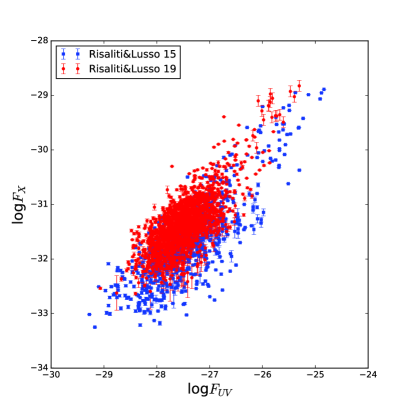
Figure 1.— $\log F_{X}$ vs. $\log F_{UV}$ diagram of quasars. Blue squares represent 808 data points from (Risaliti & Lusso, 2015), while the red circles represent 1598 data points from (Risaliti & Lusso, 2019).

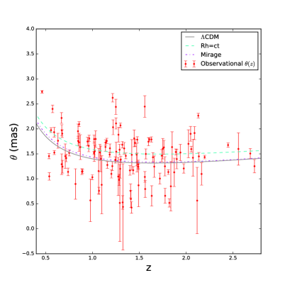
Figure 2.— Angular size $\theta$ versus redshift $z$ for the compact structure in 120 intermediate-luminosity quasars. Grey solid line, cyan dashed line and magenta dash-dot line illustrate theoretical angular size vs. redshift relation calculated from the fiducial $\Lambda$CDM cosmology with $\Omega_{m}=0.27$, the so called $\rm R_{h}=ct$ cosmology and the Mirage cosmology ($\Omega_{m}=0.27$, $w_{0}=-0.7$, $w_{1}=-1.09$), respectively. The linear size of $l_{m}=11.42\;\text{pc}$ calibrated with SN Ia in Cao et al. (2017b) was used to calculate the theoretical angular size.

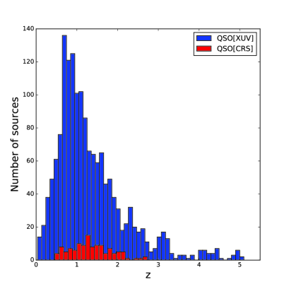
Figure 3.— The comparison of redshift distribution of the samples studied. Blue and red histograms represent redshift distributions of QSO[XUV] and QSO[CRS], respectively.

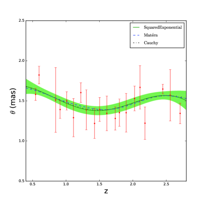
Figure 4.— Angular size vs. redshift relation reconstructed from binned data with different covariance functions and zero mean function. Red points represent median values of 20 redshift bins with width $\Delta z=0.1$ starting from the smallest redshift of the intermediate-luminosity quasars. Green solid line, blue dashed line and black dash-dot line means the reconstructed angular size with Squared Exponential, $\rm Mat\acute{e}rn$ and Cauchy covariance function, respectively. Green range means the $1\sigma$ uncertainty band of the reconstructed angular size based on the Squared Exponential convariance function.

2.2. Angular diameter distances from compact radio quasars

The angular size-redshift ($\theta-z$) relation of the compact structure in radio sources has been useful for cosmological studies. The angular size of compact sources at different redshifts $\theta(z)$ can be written as

$$\theta(z)=\frac{l_{m}}{D_{A}(z)}$$ (2)

where $l_{m}$ is the intrinsic metric length of the source and $D_{A}(z)$ is the angular diameter distance. The angular size-redshift relation was first proposed by Kellermann (1993) who attempted to estimate the deceleration parameter based on 79 compact sources obtained using Very Long Baseline Interferometry (VLBI) at 5 GHz frequency where the angular size was defined as a distance between the core and the component of $2\%$ core brightness. The method was extended by Gurvits (1994) who used 337 active galactic muclei (AGNs) observed at 2.29 GHz by Preston et al. (1985) to discuss the luminosity and redshift dependence of their characteristic size and estimate the deceleration parameter. Unlike the angular size definition of Kellermann (1993), Gurvits (1994) used the modulus of visibility $\Gamma=S_{c}/S_{t}$ to express source compactness and the characteristic angular size of radio sources can be calculated through the expression of $\theta(z)=2\sqrt{-\ln\Gamma\ln 2}/\pi B_{\theta}$ where $B_{\theta}$ is the interferometer baseline, $S_{c}$ and $S_{t}$ are correlated flux density and total flux density, respectively. Moreover, Gurvits et al. (1999) used another sample of 330 VLBI contour maps at 5 GHz collected from the literature and discussed the influence of dispersion in the “$\theta-z$” relation and these data was widely used to cosmological parameter inference (Chen & Ratra, 2003; Zhu et al., 2004). Then, Jackson et al. (2004) tried to establish a plausible model to understand the physical meaning of such standard rulers using the compilations from Gurvits (1994); Gurvits et al. (1999).

Phenomenological dependence of the intrinsic length in Eq. (2) on the source luminosity and the redshift can be expressed as

$$l_{m}=lL^{\rho}(1+z)^{n}$$ (3)

where $l$ is the linear size scaling factor, $\rho$ and $n$ power-law exponents capture the dependence of the intrinsic length on source luminosity and redshift, respectively. In Preston et al. (1985), 917 radio sources were detected in several VLBI studies at 2.29 GHz according to 1398 candidates selected from previous surveys while some of them did not have the necessary information like the total flux density or redshift. Then, Jackson & Jannetta (2006) complemented these data with relevant information obtained from the NASA/IPAC Extragalactic Database and contemporaneous radio measurements catalogue. The resulting compilation comprised 613 object in total. However, it was a mixture of extragalactic objects including quasars, BL Lacertae objects, radio galaxies, etc. As discussed in Cao et al. (2015), the dependence of the linear size on luminosity and redshift is different in different class of objects. This conclusion was based on the Gurvits (1994) sample under assumption of standard $\Lambda$CDM cosmological model and with best fitted parameters obtained from Planck/WMAP observations. Applying the selection criteria of flat spectral index $-0.38\leq\alpha\leq 0.18$ and luminosity in the range of $10^{27}\;\text{W/Hz}\leq L\leq 10^{28}\;\text{W/Hz}$ to the Jackson & Jannetta (2006) sample, Cao et al. (2017a, b) identified a sample of 120 intermediate-luminosity quasars displaying negligible dependence on both source luminosity and redshift ($|\rho|\approx 10^{-4},|n|\approx 10^{-3}$). Therefore the compact structure sizes of these quasars are potentially promising standard rulers with multi-frequency VLBI observations (Cao et al., 2018). This subsample was successfully used in cosmological applications including the measurements of speed of light (Cao et al., 2017b, 2020) and cosmic curvature at different redshifts (Cao et al., 2019), cosmological model selection (Li et al., 2017; Ma et al., 2017), testing modified gravity models (Qi et al., 2017; Xu et al., 2018) and interacting dark energy models (Zheng et al., 2017). We will use it in the present paper and denote it by the abbreviation QSO[CRS]. Fig. 2 displays the angular size-redshift relation in this sample (red points with corresponding error bars).

2.3. The test of CDDR

The validity of CDDR can be tested by the determination of the $\eta(z)$ parameter:

$$\eta(z)=\frac{D_{L}(z)}{D_{A}(z)(1+z)^{2}}$$ (4)

where $\eta(z)=1$ corresponds to the standard Etherington reciprocity relation and any statistically significant deviations from it might signal the violation of any of the underlying assumptions. In our study we derived luminosity distances and angular diameter distances from QSO[XUV] and QSO[CRS], respectively. The advantage of this approach is in covering the wide redshift range and using the same population of objects (the quasars) in the assessment of two different distance measures. As discussed above, we used the compilation of angular size measurements of compact radio quasar to determine the angular diameter distance, and the quasar flux measurements in X-ray and UV bands which can be used to derive the luminosity distance. Redshift distributions of QSO[XUV] and QSO[CRS] samples are shown in Fig. 3. One can see that the redshift range probed by quasars is considerable and that two samples overlap sufficiently with each other.

In order to test the CDDR, we use four parameterizations of $\eta(z)$

$$\eta(z)=\left\{\begin{array}[]{l@{\hspace{1cm}}l}1+\eta_{0}\;z\hfil\hskip 28.45274pt\\ (1+z)^{\eta_{1}}\hfil\hskip 28.45274pt\\ 1+\eta_{2}\;\frac{z}{1+z}\hfil\hskip 28.45274pt\\ 1+\eta_{3}\;{\rm ln}(1+z)\hfil\hskip 28.45274pt\\ \end{array}\right.$$ (5)

There is no guidance from the theory which parametrization could be distinguished, but mutually consistent results for different parameterizations would strengthen the robustness of the conclusion.

From Eq. (1), theoretical expression of the luminosity distance can be reformulated as

$$D_{L}^{QSO[XUV]}(z) = 10^{(\log F_{X}-\gamma\log F_{UV})/(2\gamma-2)}$$ (6)

$$\times 10^{-[\log(4\pi)/2+\beta/(2\gamma-2)]}$$

In principle, the parameters $\gamma$ and $\beta$ can be fitted to different cosmological models in a manner analogous to the Type Ia Supernova light-curve fitting (Betoule et al., 2014; Melia, 2019). Other approach is to derive the slope $\gamma$ from the nonlinear relation between the UV and X-ray luminosities with sub-samples in different redshift intervals and calibrate the $\beta$ intercept on external probes like SN Ia (Risaliti & Lusso, 2015). Risaliti & Lusso (2015) demonstrated that the $\gamma$ parameter does not display any significant redshift evolution pattern but is close to a certain average value. While it is not possible to test the redshift dependence of the intercept parameter $\beta$, one can anchor it by means of the cross-calibration on the SN Ia sample having redshifts overlapping with quasars. Following this method, we assumed $\gamma=0.633\pm 0.002$ derived in Risaliti & Lusso (2019) but we treated the intercept $\beta$ as a free parameter.

Similarly, according to Eq. (2), angular diameter distances can be calculated from observed angular sizes as

$$D_{A}^{QSO[CRS]}(z)=l_{m}/\theta(z)$$ (7)

and we also treated the length scale $l_{m}$ as a free parameter. In order to test the CDDR using different samples one should use a redshift matching criterion $\Delta z<0.005$ (Li et al., 2011; Liao et al., 2016). However, it turned out difficult to fulfill this criterion in order to compare distances derived from QSO[XUV] and QSO[CRS] directly. Therefore, proceeding in a similar manner as Li et al. (2018), we reconstruct QSO[CRS] angular size as a function of redshift from the binned data. The angular size of intermediate-luminosity quasars was grouped into 20 redshift bins of width $\Delta z=0.1$ starting from the smallest redshift of this sample. Median values of angular size plotted against the mean redshift in each bin are shown in Fig.4. The python package GaPP based on Gaussian Processes (Seikel et al., 2012) was used for the reconstruction process which depends on the mean function and the covariance function $k(x,\tilde{x})$. In order to discuss the influence of the choice of these two prior functions, we studied four mean functions and three covariance functions. The prior mean functions which we discussed are the following: zero mean function, the theoretical function of angular size calculated from the angular diameter distance under the assumption of three cosmological models: flat $\Lambda$CDM with $\Omega_{m}=0.27$, so called $R_{h}=ct$ Universe (Melia & Shevchuk, 2012), and a Mirage model with $\Omega_{m}=0.27$, $w_{0}=-0.7$ and $w_{1}=-1.09$ (Shafieloo et al., 2012). The linear size scaling factor $l_{m}=11.42\;\rm pc$ was assumed as calibrated with SN Ia in Cao et al. (2017b). These functions (except the zero mean function) are shown in Fig.2. There are many possible covariance functions and we studied three most popular ones. They comprise: the Squared Exponential function

$$k(x,\tilde{x})=\sigma_{f}^{2}\exp\left(-\frac{(x-\tilde{x})^{2}}{2\ell^{2}}\right)$$ (8)

the $\rm Mat\acute{e}rn$

$$k(x,\tilde{x})=\sigma_{f}^{2}\exp\left[-\frac{\sqrt{3}|x-\tilde{x}|}{\ell}\right]\left(1+\frac{\sqrt{3}|x-\tilde{x}|}{\ell}\right)$$ (9)

and Cauchy covariance function

$$k(x,\tilde{x})=\sigma_{f}^{2}\frac{\ell}{(x-\tilde{x})^{2}+\ell^{2}}$$ (10)

where $\sigma_{f}$ and $\ell$ are hyperparameters that control the amplitude of deviation from the mean function and the typical length scale in x-direction, respectively. It is instructive to discuss the effects of the mean function and covariance function selection (prior assumptions) on the reconstruction. In order to show the impact of covariance function choice, we fixed the zero mean and preformed reconstruction with three different covariance functions mentioned above. The result obtained under assumption of Squared Exponential covariance function is illustrated in Fig. 4, where the green solid line represents the reconstructed $\theta(z)$ relation and green region around it represents $1\sigma$ uncertainty band. The blue dashed line and black dash-dot line represent the reconstructed $\theta(z)$ relation with the Mat$\rm\acute{e}$rn and Cauchy covariance functions, respectively. Their uncertainty bands are not shown in order not to blur the picture since they are similar to the one displayed. One can see that differences between reconstructions performed with different choice of covariance function are insignificant. Similarly, we checked sensitivity of reconstructions with respect to the choice of the mean function fixing the covariance as Squared Exponential one and using three main functions mentioned above. It turned out that the impact of mean function choice on the reconstruction was even smaller that that of the covariance function. Therefore for further calculations we assumed the zero mean function and the Squared Exponential covariance function to get the reconstructed $\theta(z)$ function (i.e. the green line and region in Fig.4). Using this reconstructed relation we were able to have a one-to-one matching between the QSO[CRS] angular diameter distance and the QSO[XUV] luminosity distance at the same redshift.

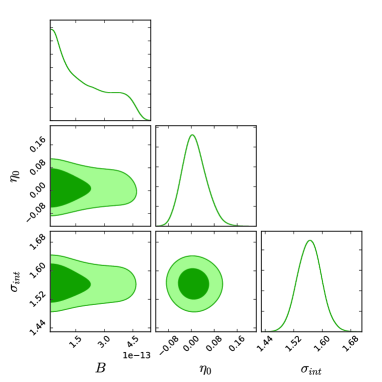
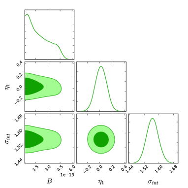
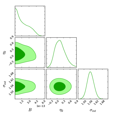
Figure 5.— Two dimensional and marginalized distributions of the nuisance parameter $B$, the CDDR validity parameter $\eta$ and the intrinsic scatter $\sigma_{int}$ in four parameterizations of $\eta(z)$ according to Eq. (5).

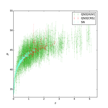
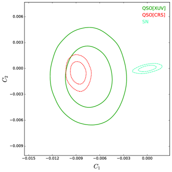
Figure 6.— Distance modulus and confidence contours of the crossing statistics hyperparameters based on Union2.1 SN, QSO[XUV] and QSO[CRS] data compilations. The QSO[CRS] linear size parameter $l=11.42\pm 0.28\;pc$ and the QSO[XUV] intercept parameter $\beta=8.24\pm 0.02$ were used to get corresponding distance modulus and both of them were calibrated from the same SN compilation (Union2.1).

Now the observed CDDR parameter $\eta_{obs}(z)$ can be expressed as

$$\eta_{obs}(z) = \frac{D_{L}^{QSO[XUV]}(z)}{D_{A}^{QSO[CRS]}(z)(1+z)^{2}}$$ (11)

$$= B(1+z)^{-2}\theta(z)10^{(\log F_{X}-\gamma\log F_{UV})/(2\gamma-2)}$$

where $B=[l_{m}\;10^{[\log(4\pi)/2+\beta/(2\gamma-2)]}]^{-1}$ is the nuisance parameter containing both the linear size scaling factor $l_{m}$ and the intercept $\beta$. Concerning the uncertainty budget, we considered uncertainties of $\theta(z)$, $\log F_{X}$, $\gamma$, and an intrinsic scatter $\sigma_{int}$ which is meant to capture the global intrinsic dispersion $\delta$ in QSO[XUV] data and other unconsidered uncertainties. Intrinsic scatter was treated as a free parameter. The uncertainty of ${\log F_{UV}}$ is negligible compared to the uncertainty of ${\sigma_{\log F_{X}}}$ hence we ignored it. So the total uncertainty of $\eta(z)$ can be expressed as

$$\sigma_{\eta}=\sqrt{\sigma_{\theta}^{2}+\sigma_{\gamma}^{2}+\sigma_{\rm logF_{X}}^{2}+\sigma_{int}^{2}}$$ (12)

where the subsequent components are following:

$$\sigma_{\theta} = \frac{B}{(1+z)^{2}}{10^{(\log F_{X}-\gamma\log F_{UV})/(2\gamma-2)}}d{\theta(z)}$$

$$\sigma_{\gamma} = \frac{B}{(1+z)^{2}}\theta(z){10^{(\log F_{X}-\gamma\log F_{UV})/(2\gamma-2)}}$$

$$\times {\ln 10}\frac{\log F_{UV}-\log F_{X}}{2(\gamma-1)^{2}}d{\gamma}$$

$$\sigma_{\log F_{X}} = \frac{B}{(1+z)^{2}}\theta(z){10^{(\log F_{X}-\gamma\log F_{UV})/(2\gamma-2)}}$$ (13)

$$\times {\ln 10}\frac{1}{2(\gamma-1)}d{\log F_{X}}$$

Free parameters in our calculations included: the nuisance parameter $B$ (in units of $10^{-13}$), the CDDR parameters $\eta_{i}$ ($i=0,...,3$) corresponding to four parametrizations of Eq. 5 and the intrinsic scatter parameter $\sigma_{int}$. We fitted the free parameters by maximizing the likelihood function

$$\mathcal{L}({\bf{p}})=\prod\frac{1}{\sqrt{2\pi}\sigma_{\eta}}{\rm exp}\left[-\frac{1}{2}\frac{(\eta_{obs}-\eta_{th})^{2}}{\sigma_{\eta}^{2}}\right]$$ (14)

using the Python package of $\bf{emcee}$ (Foreman-Mackey, 2013) to do the Markov Chain Monte Carlo analysis. We assumed the following uniform priors for these parameters: $P(B)=U[0,1]$, $P(\eta_{0})=U[-1,1]$, $\sigma_{int}=U[0,2]$.

3. Results and Discussion

The best fitted parameter values and corresponding $1\sigma$ uncertainties are listed in Table .1 and shown in Fig. 5. One can see that there is no evidence for the CDDR violation in none of the parameterizations considered. Hence the conclusion of CDDR validity seems robust. This is consistent with the conclusions of other works including the comparison between luminosity distances derived form SN Ia and angular diameter distances to galaxy clusters (Holanda et al., 2010; Li et al., 2011), gas mass fraction of clusters (Goncalves et al., 2015), Baryon Acoustic Oscillations (Wu et al., 2015) at low redshifts, strong gravitational lensing systems (Liao et al., 2016), gamma-ray bursts (Holanda et al., 2017) or compact radio sources (Li et al., 2018). Recently some authors made forecasts concerning CDDR testing based on the simulated luminosity distances of standard sirens detectable in the future by the Einstein Telescope combined with strong gravitational lensing systems (Yang et al., 2019) or simulated compact radio quasars (Qi et al., 2019). Assuming $\eta(z)=1+\eta_{0}z$ parametrization they shown that the 1$\sigma$ uncertainty level can reduced to 0.035 and 0.0093, respectively. Using a single population of objects, Holanda et al. (2012) tested the cosmic distance duality at low redshift ($0.14<z<0.89$) according to the measurements of the gas mass fraction of galaxy clusters from Sunyaev-Zeldovich and X-ray surface brightness. They obtained the following results: $\eta_{0}=-0.06\pm 0.16$ and $\eta_{2}=-0.07\pm 0.24$ after excluding objects with questionable reduced $\chi^{2}$. Comparing to other independent approaches mentioned above, our method is competitive and our results support the validity of CDDR. Underlying our approach is the use of the same kind of objects – quasars – visible at high redshifts. This might alleviate some systematics coming from different physical properties of different populations of objects. Even though the accuracy of our results is poorer than that forecasted from the simulated data, yet our method provided constraints on CDDR violation more stringent than other currently available results based on real observational data.

The linear size parameter $l_{m}$ and the intercept $\beta$ are hard to determine precisely due to, respectively: the ambiguous interpretation of the compact structure size in radio quasars and the variation of slope in X-UV luminosity relation of quasars. Therefore, it is necessary to calibrate the values of $l_{m}$ and $\beta$ separately before using them to investigate cosmological parameters. The linear size parameter $l_{m}$ was previously calibrated with Type Ia SN (Cao et al., 2017b) and with Hubble parameters (Cao et al., 2017a), while the calibration of $\beta$ was discussed by Risaliti & Lusso (2015). Being focused on the CCDR parameters, we entangled $l_{m}$ and $\beta$ in a single nuisance parameter $B$. However, we have checked the influence of $l_{m}$ and $\beta$ on the CDDR parameters using the priors based on the above mentioned calibrations. It turned out that it very slightly modified the results presented in this paper. The advantage of the approach we taken here (i.e. using a nuisance parameter $B$) was that we avoided external calibrations which might be cosmological model dependent and introduce tacit assumptions leading to circularity of reasoning.

Our result, i.e. confirmation of CDDR validity suggest to use it as an assumption and discuss the consistency between distances derived from QSO[XUV] and QSO[CRS]. The proper framework for this purpose is set by the Crossing Statistics approach as introduced in (Shafieloo et al., 2013) (for more detailed description of the method see the references therein). Instead of smooth reconstructed distances we will use distance moduli $\mu_{smooth}$ derived from them. Following (Shafieloo et al., 2013) we represent the Crossing function by a second order Chebyshev polynomial

$$F_{II}(C_{1},C_{2},z)=1+C_{1}(\frac{z}{z_{max}})+C_{2}[2(\frac{z}{z_{max}})^{2}-1]$$ (15)

where $C_{1}$, $C_{2}$ are the hyperparameters and $z_{max}$ is the maximum redshift in the data compilations. Then, we fit the data to the functions of $\mu_{smooth}^{F_{II}}(z)=\mu_{smooth}\times F_{II}(C_{1},C_{2},z)$ based on $\chi^{2}$ statistics. For comparison, we first use Union2.1 SN Ia data (Suzuki et al., 2012) to reconstruct $\mu_{smooth}$ using Gaussian processes and then use this function to fit SN data itself, QSO[XUV] data and QSO[CRS] data. The QSO[CRS] linear size parameter $l=11.42\pm 0.28\;pc$ and the QSO[XUV] intercept parameter $\beta=8.24\pm 0.02$ were used to derive corresponding distances and both of them were calibrated from the same supernovae compilation (Union2.1). The final results of the hyperparameters fitting are shown in Fig.6. The confidence contours of $C_{1}^{SN}$ and $C_{2}^{SN}$ is centered around the (0,0) point as expected because the prior of the smooth mean function is derived from supernovae data itself. According to the same smooth mean function, the confidence contours of ($C_{1}^{QSO[CRS]}$, $C_{2}^{QSO[CRS]}$) and ($C_{1}^{QSO[XUV]}$, $C_{2}^{QSO[XUV]}$) turn out inconsistent with ($C_{1}^{SN}$, $C_{2}^{SN}$) while having a good overlap region with each other. Inconsistency between supernova and QSO[CRS](or QSO[XUV]) data suggest that it might be some systematics in these data not properly accounted for. Moreover, this inconsistency implies that the cosmological models best fitted to these data compilations may be different. This issue is very important and will be investigated in a future work. Let us note that the QSO[CRS] and QSO[XUV] data, both having large intrinsic dispersions are hard to smooth directly except by using the redshift binned data and this process may result with systematics and impact the result. It is remarkable that the confidence contours of QSO[CRS] and QSO[XUV] are consistent with each other which further supports the validity of our method.

Table 1Results of CDDR test using four parameterizations according to Eq. (5). $B$ is the nuisance parameter containing both the linear size $l_{m}$ of QSO[CRS] standard rulers and the intercept $\beta$ for QSO[XUV] standard candles, $\eta_{i}$ is the CDDR parameter and $\sigma_{int}$ is the intrinsic scatter.

${\rm\eta(z)}$	$B\times 10^{-13}$	$\eta_{i}$	$\sigma_{int}$
${\rm 1+\eta_{0}z}$	$1.61^{+1.97}_{-1.12}$	$0.01^{+0.04}_{-0.04}$	$1.56^{+0.03}_{-0.03}$
${\rm(1+z)^{\eta_{1}}}$	$1.66^{+1.84}_{-1.11}$	$0.02^{+0.09}_{-0.09}$	$1.57^{+0.03}_{-0.03}$
${\rm 1+\eta_{2}z/(1+z)}$	$1.48^{+1.74}_{-1.02}$	$0.13^{+0.26}_{-0.21}$	$1.56^{+0.03}_{-0.03}$
${\rm 1+\eta_{3}ln(1+z)}$	$1.65^{+1.84}_{-1.15}$	$0.04^{+0.10}_{-0.09}$	$1.57^{+0.03}_{-0.03}$

4. Conclusion

As a fundamental relation rooted in the very ground of modern cosmology, i.e., the validity of General Relativity (or more general – the metric theory of gravity), the CDDR is very successful in explaining many observational facts concerning our Universe (Planck Collaboration, 2018). However, its slight violations might also signal non-conservation of photon number on the way from the source to the observer. Such effect could be due to photons decaying to axions or due to less exotic causes like absorption by intergalactic medium. Therefore it is very important to test it on available observational material. So far it has been tested mainly at lower redshifts where the observational measurements are abundant and it started to be extended to higher redshifts (Liao et al., 2016; Holanda et al., 2017). Interesting approach is to use for this purpose the gravitational wave measurements of coalescing compact binaries (Yang et al., 2019; Qi et al., 2019). However, we should wait for the future third generation GW detectors until the statistics and the redshift coverage will be sufficient to get competitive results.

In this paper, we proposed to test the CDDR using high redshift quasars which can provide both luminosity distances and the angular diameter distances. The angular diameter distances we used come from the angular size measurements of compact structures in intermediate-luminosity radio quasars (Cao et al., 2017a) and the luminosity distances come from the non-linear relation between the UV and X-ray emission (Risaliti & Lusso, 2019). We used four different cosmic distance duality relation parameterizations: linear in redshift $\eta(z)=1+\eta_{0}z$, power-law $\eta(z)=(1+z)^{\eta_{1}}$, linear in scale factor $\eta(z)=1+\eta_{2}\;z/(1+z)$, and logarithmic $\eta(z)=1+\eta_{3}\;{\ln}(1+z)$. The linear size parameter $l_{m}$ of compact structure and the intercept parameter $\beta$ in X-UV relation should in principle be calibrated independently. However, it is currently very hard to achieve due to lack of solid physical understanding of the X-UV relation and why the intermediate-luminosity quasars could be standardizable rulers. Moreover, external calibrators might introduce other systematics and hidden assumptions influencing the results. In order to circumvent these problems, we entangled both $l_{m}$ and $\beta$ parameter into one external parameter $B$, which was furthermore treated as a free parameter to fit and marginalized over. Our results, which support the validity of the CDDR at $z\sim 3$, turned out to be more competitive than other approaches. Given the wealth of available high-$z$ quasars in the future, we may be optimistic about detecting possible deviation from the CDDR within our observational volume. Such accurate model-independent measurements of the CDDR can become a milestone in precision cosmology.

This work was supported by the National Key R&D Program of China No. 2017YFA0402600; the National Natural Science Foundation of China under grant Nos. 11690023, 11633001 and 11920101003; the Strategic Priority Research Program of the Chinese Academy of Sciences, grant No. XDB23000000; Beijing Talents Fund of Organization Department of Beijing Municipal Committee of the CPC; the Interdiscipline Research Funds of Beijing Normal University; and the Opening Project of Key Laboratory of Computational Astrophysics, National Astronomical Observatories, Chinese Academy of Sciences. This work was performed in part at Aspen Center for Physics, which is supported by National Science Foundation grant PHY-1607611. This work was partially supported by a grant from the Simons Foundation. M.B. is grateful for this support.

References

- Betoule et al. (2014) Betoule, M., et al. 2014, A&A, 568, 22
- Bisogni et al. (2018) Bisogni, S., Risaliti, G. & Lusso, E. 2018, FrASS, 4, 68
- Cao & Liang (2011) Cao, S., & Liang, N. 2011, RAA, 11, 1199
- Cao & Zhu (2011) Cao, S., & Zhu, Z.-H. 2011, China Series G, 54, 12
- Cao et al. (2015) Cao, S., Biesiada, M., Zheng, X. G., Zhu, Z.-H. 2015, ApJ, 806, 66
- Cao et al. (2016) Cao, S., et al. 2016, MNRAS, 461, 2192
- Cao et al. (2017a) Cao, S., Zheng, X. G., Biesiada, M., et al. 2017a, A&A, 606, A15
- Cao et al. (2017b) Cao, S., Biesiada, M., Jackson, J., et al. 2017b, JCAP, 02, 012
- Cao et al. (2018) Cao, S., Biesiada, M., Zheng, X. G., et al. 2018, EPJC, 78, 749
- Cao et al. (2019) Cao, S., Qi, J. Z., Biesiada, M., et al. 2019, Physics of the Dark Universe, 24, 100274
- Cao et al. (2020) Cao, S., Qi, J. Z., Biesiada, M., Liu, T. H., Zhu, Z.-H. 2020, ApJL, 888, L25
- Chen & Ratra (2003) Chen, G. & Ratra, B. 2003, ApJ, 582, 586
- Costa et al. (2015) Costa, S. S., Busti, V. C., & Holanda, R. F. L. 2015, JCAP, 10, 061
- Elvis & Karovska (2002) Elivs, M., & Karovska, M. 2002, ApJL, 581, L67
- Etherington (1933) Etherington, I. M. H. 1933, Phil.Mag., 15, 761
- Etherington (2007) Etherington, I. M. H. 2007, Gen.Relativ.Gravit., 39, 1055
- Foreman-Mackey (2013) Foreman-Mackey, D., Hogg, D. W., Lang, D., & Goodman, J. 2013, PASA, 125,306
- Goncalves et al. (2015) Goncalves, R., Bernui, A., Holanda, R. F. L., & Alcaniz, J. 2015, A&A, 573, A88
- Gurvits (1994) Gurvits, L. I. 1994, ApJ, 425, 442
- Gurvits et al. (1999) Gurvits, L. I., Kellermann, K. I., & Frey, S. 1999, A&A, 342, 378
- Holanda et al. (2010) Holanda, R. F.L., Lima, J. A. S., Ribeiro, M. B. 2010, ApJL, 722, L233
- Holanda et al. (2012) Holanda, R. F.L., Goncalves, R. S., & Alcaniz, J. S. 2012, JCAP, 06, 022
- Holanda et al. (2017) Holanda, R. F.L., Busti, V. C., Lima, F. S., & Alcaniz, J. S. 2017, JCAP, 09, 039
- Jackson et al. (2004) Jackson, J. C. 2004, JCAP, 11, 007
- Jackson & Jannetta (2006) Jackson, J. C., & Jannetta, A. L. 2006, JCAP, 11, 002
- Kellermann (1993) Kellermann, K. I. 1993, Nature, 361, 134
- La Franca et al. (2014) La Franca, F., Bianchi, S., Ponti, G., Branchini, E., & Matt, G. 2014, ApJL, 787, L12
- Li et al. (2017) Li, X. L., Cao, S., Zheng, X. G., et al. 2017, EPJC, 77, 677
- Li et al. (2018) Li, X., & Lin, H. N. 2018, MNRAS, 474, 313
- Li et al. (2011) Li, Z. X., Wu, P. X., Yu, H. W. 2011, ApJL, 729, L14
- Liao et al. (2015) Liao, K., Avgoustidis, A., & Li, Z. X. 2015, PRD, 92, 123539
- Liao et al. (2016) Liao, K., Li, Z. X., Cao, S. et al. 2016, ApJ, 822, 74
- Lusso & Risaliti (2016) Lusso, E., & Risaliti, G. 2016, ApJ, 819, 154
- Melia & Shevchuk (2012) Melia, F., & Shevchuk, A. S. H. 2012, MNRAS, 419, 2579
- Ma et al. (2017) Melia, Y. B., Zhang, J., Cao, S., et al. 2017, EPJC, 77, 891
- Melia (2019) Melia, F. 2019, MNRAS, 489, 517
- Planck Collaboration (2018) Planck Collaboration, arXiv:1807.06209
- Preston et al. (1985) Preston, R. A., et al. 1985, AJ, 90, 1599
- Qi et al. (2017) Qi, J. Z., Cao, S., Biesiada, M., et al. 2017, EPJC, 77, 502
- Qi et al. (2019) Qi, J. Z., et al. 2019, Physics of the Dark Universe, 26, 100338
- Qi et al. (2019) Qi, J. Z., Cao, S., Zheng, C. F., et al. 2019, PRD, 99, 063507
- Rana et al. (2017) Rana, A., Jain, D., Mahajan, S., Mukherjee, A., Holanda, R. F. L. 2017, JCAP, 07, 010
- Risaliti & Lusso (2015) Risaliti, G., & Lusso, E. 2015, ApJ, 815, 33
- Risaliti & Lusso (2017) Risaliti, G., & Lusso, E. 2017, AN, 338, 329
- Risaliti & Lusso (2019) Risaliti, G., & Lusso, E. 2019, Nature Astronomy, 3, 272
- Seikel et al. (2012) Seikel, M., Clarkson, C., & Smith, M. 2012, JCAP, 1206, 036
- Shafieloo et al. (2012) Shafieloo, A., Kim, A. G., & Linder, E. V. 2012, PRD, 85, 123530
- Shafieloo et al. (2013) Shafieloo, A., Majumdar, S., Sahni, V., & Starobinsky, A. A. 2013, JCAP, 04, 042
- Suzuki et al. (2012) Suzuki, N., Rubin, D., Lidman, C., et al. 2012, ApJ, 746, 85
- Wang et al. (2013) Wang, J.M., Du, P., Valls-Gabaud, D., Hu, C., & Netzer, H., 2013, PRL, 110, 081301
- Watson et al. (2011) Watson, D., Denney, K. D., Vestergaard, M., & Davis, T. M. 2011, ApJL, 740, L49
- Wu et al. (2015) Wu, P. X., Li, Z. X., Yu, H. 2015, PRD, 92, 023520
- Xu et al. (2018) Xu, T. P., Cao, S., Qi, J. Z., et al. 2018, JCAP, 06, 042
- Yang et al. (2013) Yang, X., Yu, H. R., Zhang, T. J. 2013, JCAP, 06, 007
- Yang et al. (2019) Yang, T., Holanda, R. F. L., & Hu, B. 2019, Astroparticle Physics, 108, 57
- Zheng et al. (2017) Zheng, X. G., Biesiada, M., Cao, S., et al. 2017, JCAP, 10, 030
- Zhu et al. (2004) Zhu, Z.-H., Fujimoto, M. K., & He, X. T. 2004, A&A, 417, 833