What Can We Learn by Combining the Skew Spectrum and the Power Spectrum?

Abstract

Clustering of the large scale structure provides complementary information to the measurements of the cosmic microwave background anisotropies through power spectrum and bispectrum of density perturbations. Extracting the bispectrum information, however, is more challenging than it is from the power spectrum due to the complex models and the computational cost to measure the signal and its covariance. To overcome these problems, we adopt a proxy statistic, skew spectrum which is a cross-spectrum of the density field and its quadratic field. By applying a large smoothing filter to the density field, we show the theory fits the simulations very well. With the spectra and their full covariance estimated from $N$-body simulations as our “mock” Universe, we perform a global fits for the cosmological parameters. The results show that adding skew spectrum to power spectrum the $1\sigma$ marginalized errors for parameters $b_{1}^{2}A_{s},n_{s}$ and $f_{\rm NL}^{\rm loc}$ are reduced by $31\%,22\%,44\%$, respectively. This is the answer to the question posed in the title and indicates that the skew spectrum will be a fast and effective method to access complementary information to that enclosed in the power spectrum measurements, especially for the forthcoming generation of wide-field galaxy surveys.

1 Introduction

The origin of our Universe and its evolution have been extensively probed by the cosmic microwave background (CMB) anisotropies with a three decades long effort that culminated with the Planck mission [1]. The next generation of CMB observations will also provide more precise measurements of the CMB polarization anisotropies [2]. The large scale structure (LSS) of the Universe, that is, the distribution of matter and galaxies on large scales, is the result of the late-time evolution, powered by gravitational instability, of the same initial density perturbations responsible for the CMB anisotropies. Upcoming wide-field galaxy surveys, such as DESI [3], EUCLID [4] and LSST [5], are poised to provide massive amount of high-precision data carrying complementary information to that obtained from the CMB measurements.

To date, most of the cosmological information from LSS is captured using 2-point clustering statistics, such as the 2-point correlation function or the power spectrum in Fourier space. However, the large scale structure we observe at low redshift is highly non-Gaussian as a result of the non-linear growth of structures, even for Gaussian initial conditions. Further cosmological information can be obtained for the same surveys by using also higher-order statistics, such as 3-point correlation function and bispectrum [6, 7, 8, 9, 10]. In particular the bispectrum has been measured using galaxy survey data [11, 12, 13, 14] and has proven useful to break degeneracies among cosmological parameters which arise from considering the power spectrum alone [15, 16]. Future LSS surveys will enable us to reach a much larger signal-to-noise ratio for the bispectrum, providing a wealth of information, e.g., on primordial non-Gaussianity, non-linear bias and to further reduce the parameter degeneracies present at the level of the power spectrum e.g., [17] and Refs. therein.

However, extracting the information from the bispectrum is more challenging than it is from the power spectrum, due to the large number of triangle configurations and orientations. Measuring the bispectrum signal and its covariance requires a significant computational effort e.g., [18], and the comparison of theoretical models with measurements is rather complex e.g., [15, 16].

In practice, to bypass these challenges, several proxy statistics have been proposed to extract (some of) the information enclosed in the bispectrum; of particular interest are approaches that compress the bispectrum to a pseudo-power spectrum, such that the signal depends only on one wavenumber (rather than three as for the bispectrum). There are mainly two approaches: the integrated bispectrum proposed by Ref. [19] and the skew spectrum which was studied in CMB [20, 21], and then applied to LSS [22, 23, 24, 25, 26], but see also pioneering works [27, 28]. The integrated bispectrum is generated by cross correlating the position-dependent power spectrum with the mean overdensity of the corresponding subvolume. This measurement contains parts of the bispectrum information on squeezed configuration; the application of this statistic to real data can be found in Ref. [29]. The skew spectrum (and later, the weighted skew spectrum) are obtained by cross correlating the (weighted) square of a field with the field itself. This quantity has recently received renewed attention [23, 26]. Here we build on [22] and partially also on these two works, with the aim of developing the approach further and to bring it closer to a real application to observations. However, for simplicity, here we do not consider the weighted skew spectrum. In particular, we focus on prospects and possible challenges of the joint analysis of skew spectrum and power spectrum, and compare theoretical and analytical modelling to $N$-body simulations.

As a first step, we estimate the skew spectra from $N$-body simulations of the cosmological density field $\delta$ in a straightforward way by cross correlating $\delta(\bm{x})$ and $\delta^{2}(\bm{x})$, and then study the extra information that can be obtained by combining the skew spectrum and the power spectrum. We consider three main sources of (non-Gaussian) skew spectrum signal: primordial non-Gaussianity, gravitational instability and galaxy bias. The full covariance matrix for the two statistics is estimated from a large suite of $N$-body simulations. This step, although challenging, is particularly important, since an accurate estimation of the full covariance of the two quantities is a key ingredient to evaluate the added value offered by a joint analysis of the two statistics. The performance of our adopted ansatz for the likelihood function is also evaluated with a suite of simulations. All this enable us to quantify the usefulness of using skew spectrum and power spectrum jointly to constrain some key cosmological parameters. This has not been addressed before in the literatures, but it is a question worth asking before deciding whether to proceed to measure the skew spectrum from real galaxy surveys. Note that usually these type of analyses are done by Fisher matrix, which is much less computationally intensive. However, the high covariance between power spectrum and skew spectrum, and the complex properties of the skew-spectrum covariance, force us to resort to numerically computed covariance from a suite of simulations.

The rest of this paper is organized as follows. In section 2 we derive the full expression for the skew spectrum including primordial non-Gaussianity, gravitational instability, galaxy bias and redshift space distortions. We also compare the integrated bispectrum with the skew spectrum in this section. In section 3 we present measurements of the skew spectra from $N$-body simulations and introduce the covariance used in our analysis. In section 4 we list the resulting constraints using simulations and finally we conclude in section 5.

2 Methodology

This section is somewhat pedagogical and covers mostly background material, but is important to describe the methodology adopted and to define the notation used.

Let us define the over density field $\delta({\bm{x}})=\delta\rho(\bm{x})/\bar{\rho}$ where $\rho$ denotes the matter density field and $\bar{\rho}$ its (spatial) average. It is well known that the two point correlation function $\xi(r)=\langle\delta({\bm{x}})\delta({\bm{x}+\bm{r}})\rangle$, where $\langle.\rangle$ denotes the ensemble average is related to the power spectrum $P(k)$ via a Fourier transform. Similarly, the 3-point correlation function,

$$\xi^{(3)}(\bm{x_{1}},\bm{x_{2}},\bm{x}_{3})=\left\langle\delta\left(\bm{x}_{1}\right)\delta\left(\bm{x}_{2}\right)\delta\left(\bm{x}_{3}\right)\right\rangle,$$ (2.1)

is related to the bispectrum $B\left(\bm{k}_{1},\bm{k}_{2},\bm{k}_{3}\right)$ via,

$$\xi^{(3)}\left(\bm{x}_{1},\bm{x}_{2},\bm{x}_{3}\right)=(2\pi)^{3}\int_{\bm{k}_{1}}\int_{\bm{k}_{2}}\int_{\bm{k}_{3}}\delta^{D}\left(\bm{k}_{1}+\bm{k}_{2}+\bm{k}_{3}\right)B_{m}\left(\bm{k}_{1},\bm{k}_{2},\bm{k}_{3}\right){\rm e}^{\rm{i}\left[\bm{k}_{1}\cdot\bm{x}_{1}+\bm{k}_{2}\cdot\bm{x}_{2}+\bm{k}_{3}\cdot\bm{x}_{3}\right]},$$ (2.2)

where the Dirac delta $\delta^{D}$ ensures that the wavevectors correspond to the three sides of a triangle. The bispectrum is an effective statistic to recover information not present in power spectrum, but it is challenging to measure form large scale structure data.

The (auto) skew spectrum is defined from the cross correlation of the square of the field, $\delta^{2}$ with the $\delta$ field itself. The squaring operation is intrinsically a configuration space operation (very similar to local non-Gaussianity). For this reason we find it natural to start from configuration space.

In fact, let us assume $\bm{x}_{3}$ in Eq.(2.1) is located at the same point as $\bm{x}_{1}$:

$$\xi^{(3)}(\bm{x_{1}},\bm{x_{1}},\bm{x}_{2})=\xi^{(s)}(|\bm{x}_{1}-\bm{x}_{2}|)\equiv\xi^{(s)}(x_{12})\,,$$ (2.3)

where we have recognised the skew correlation function, $\xi^{(s)}$, and we have used the fact that the cosmological principle imposes that $\xi^{(s)}$ depends only on the magnitude of the separation vector. The Fourier transform of $\xi^{(s)}$ is the skew spectrum [22, 23, 24, 25, 26].

We can now interpret the skew spectrum in light of the bispectrum. Following Ref. [30] we have,

$$\xi^{(s)}(x_{12})=\int\frac{d^{3}\bm{k}_{12}}{(2\pi)^{3}}\int\frac{d^{3}\bm{k}_{1}}{(2\pi)^{3}}B_{m}(k_{1},k_{2},|\bm{k}_{12}|){\rm e}^{\rm{i}\bm{k}_{12}\bm{x}_{12}},$$ (2.4)

where $\bm{x}_{12}\equiv\bm{x}_{1}-\bm{x}_{2}$ and $\bm{k}_{12}\equiv\bm{k}_{1}+\bm{k}_{2}$. The Fourier transform of this function yields the skew spectrum which can be written as

$$P_{m}^{(s)}(k)=\int\frac{d^{3}\bm{q}}{(2\pi)^{3}}B_{m}(k,q,|\bm{q}-\bm{k}|)=\int_{-1}^{1}d\mu\int\frac{d{q}}{(2\pi)^{2}}q^{2}B_{m}(k,q,\alpha(\mu)),$$ (2.5)

we have adopted the replacement: $\bm{k}_{12}\rightarrow\bm{k},\bm{k}_{1}\rightarrow\bm{q},\bm{k}_{2}\rightarrow\bm{\alpha}$ where $\mu=\bm{k}\cdot\bm{q}/kq$, and $\alpha=\sqrt{q^{2}+k^{2}-2\mu kq}$. The skew spectrum encloses information beyond Gaussianity. Now we consider three main sources of non-Gaussianity in real space: primordial non-Gaussianity, non-Gaussianity from gravitational instability and non-Gaussianity from galaxy bias. We begin by discussing these three effects separately, see also Ref. [22, 23, 26].

2.1 Primordial Non-Gaussianity

The skew spectrum on large scales is sensitive to the statistical properties of the primordial fluctuations. For example, non-Gaussianity of the local type is given by [31, 32, 33, 34],

$$\Phi(\bm{x})=\Phi_{G}(\bm{x})+f_{\rm NL}^{\rm{loc}}\left[\Phi_{G}^{2}(\bm{x})-\left\langle\Phi_{G}^{2}(\bm{x})\right\rangle\right],$$ (2.6)

where $\Phi(\bm{x})$ denotes the Bardeen’s curvature perturbation during the matter era, $\Phi_{G}(\bm{x})$ is a Gaussian field and $f_{\rm NL}^{\rm{loc}}$ is a constant which characterizes the amplitude of primordial non-Gaussianity. The leading contribution to the bispectrum of the curvature field is given by

$$B_{\Phi}\simeq 2f_{\rm NL}^{\rm{loc}}\left[P_{\Phi}(k_{1})P_{\Phi}(k_{2})+\rm cyc.\right],$$ (2.7)

where $P_{\Phi}(k)=\left\langle\Phi(k)\Phi^{*}(k)\right\rangle$. For the local type non-Gaussianity, most of the signal is concentrated in the so-called squeezed triangular configurations, $k_{1}\ll k_{2},k_{3}$.

Density fluctuations in Fourier space, $\delta(k)$, are related to the curvature perturbations,

$$\delta(k)=M(k,a)\Phi(k);~{}M(k,a)=\frac{2k^{2}T(k)D(a)}{3\Omega_{m}H_{0}^{2}},$$ (2.8)

where $a$ is the scale factor, $H_{0}$ is the current Hubble constant, $\Omega_{m}$ is the current matter energy density parameter, $T(k)$ is the matter transfer function and $D(a)$ is the growth factor. This allows us to write the contribution to the primordial matter bispectrum as

$$B_{m,I}(k_{1},k_{2},k_{3})=M(k_{1})M(k_{2})M(k_{3})B_{\Phi}(k_{1},k_{2},k_{3})\,$$ (2.9)

here we have omitted $a$ for brevity. The matter skew spectrum caused by the primordial non-Gaussianity is

$$P_{m,I}^{(s)}(k)=2f_{\rm NL}^{\rm loc}M(k)P_{\Phi}(k)\int_{-1}^{1}d\mu\int\frac{d{q}}{(2\pi)^{2}}q^{2}M(q)P_{\Phi}(q)M(\alpha)\left[2+\frac{P_{\Phi}(\alpha)}{P_{\Phi}(k)}\right].$$ (2.10)

There are other non-Gaussian templates, motivated by general single-field models of inflation, yielding bispectra such as equilateral model $B_{\Phi}^{\rm eq}=6f_{\rm NL}^{\rm eq}F^{\rm eq}$ [35, 36] and orthogonal model $B_{\Phi}^{\rm or}=6f_{\rm NL}^{\rm or}F^{\rm or}$ [37], where

$$F^{\rm eq}\simeq-\left(P_{\Phi}\left(k_{1}\right)P_{\Phi}\left(k_{2}\right)+2\rm{cyc.}\right)-2\left[P_{\Phi}\left(k_{1}\right)P_{\Phi}\left(k_{2}\right)P_{\Phi}\left(k_{3}\right)\right]^{2/3}+\left(P_{\Phi}\left(k_{1}\right)^{1/3}P_{\Phi}\left(k_{2}\right)^{2/3}P_{\Phi}\left(k_{3}\right)+5\rm{cyc.}\right),$$ (2.11)

$$F^{\rm or}\simeq-3\left(P_{\Phi}\left(k_{1}\right)P_{\Phi}\left(k_{2}\right)+2\rm{cyc.}\right)-8\left[P_{\Phi}\left(k_{1}\right)P_{\Phi}\left(k_{2}\right)P_{\Phi}\left(k_{3}\right)\right]^{2/3}+3\left(P_{\Phi}\left(k_{1}\right)^{1/3}P_{\Phi}\left(k_{2}\right)^{2/3}P_{\Phi}\left(k_{3}\right)+5\rm{cyc.}\right).$$ (2.12)

We stress here that these are templates, their correspondence to explicit non-Gaussian models, especially in the limit of specific configurations, is not perfect. Nevertheless, as it is widespread in the literature, we work here with these templates which we sometimes refer to as shapes. The skew spectra for these non-Gaussian shapes are obtained simply as,

$$P_{m,I}^{(s)}(k)^{\rm eq(or)}=M(k)\int_{-1}^{1}d\mu\int\frac{d{q}}{(2\pi)^{2}}q^{2}M(q)M(\alpha)B^{\rm eq(or)}_{\Phi}(k,q,\alpha).$$ (2.13)

2.2 Non-Gaussianity from gravitational instability

Even for Gaussian initial conditions, the late-time non-linear gravitational evolution generates a non-zero bispectrum. At quasi-linear scales non-linear evolution of matter density fluctuations can be modelled by perturbation theory in which case the density field is expanded as [e.g., [38]]

$$\delta({\bm{k}})=\delta({\bm{k}})^{(1)}+\delta({\bm{k}})^{(2)}+\delta({\bm{k}})^{(3)}+\ldots,$$ (2.14)

here we truncate expansions at the second order, and $\delta({\bm{k}})^{(2)}$ is given by,

$$\delta({\bm{k}})^{(2)}=\int\mathrm{d}^{3}\bm{q}_{1}\mathrm{d}^{3}\bm{q}_{2}\delta_{D}\left(\bm{k}-\bm{q}_{12}\right)F_{2}\left(\bm{q}_{1},\bm{q}_{2}\right)\delta({\bm{q}_{1}})^{(1)}\delta({\bm{q}_{2}})^{(1)},$$ (2.15)

where $F_{2}(\bm{q}_{1},\bm{q}_{2})$ is the known second-order kernel of standard perturbation theory,

$$F_{2}\left(\bm{q}_{1},\bm{q}_{2}\right)=\frac{5}{7}+\frac{x}{2}\left(\frac{q_{1}}{q_{2}}+\frac{q_{2}}{q_{1}}\right)+\frac{2}{7}x^{2},$$ (2.16)

with $x\equiv{\bm{q}}_{1}\cdot{\bm{q}}_{2}/q_{1}q_{2}$.

At leading order, the gravitational instability bispectrum is

$$B_{m,G}\left(k_{1},k_{2},k_{3}\right)=2F_{2}\left(\bm{k}_{1},\bm{k}_{2}\right)P_{m,L}\left(k_{1}\right)P_{m,L}\left(k_{2}\right)+\mathrm{cyc.},$$ (2.17)

where $P_{m,L}\left(k\right)$ is the linear matter power spectrum. Hereafter, we use the subscript “$L$” to represent the linear terms. This expression for the perturbative bispectrum can of course be improved. A particularly interesting modification is the phenomenological one proposed by Ref. [39, 40], which maintains the same structure and adjusts the coefficients of Eq.(2.16) to fit $N$-body simulations. The matter skew spectrum contribution from non-linear gravitational evolution is therefore,

$$P_{m,G}^{(s)}(k)=\int_{-1}^{1}d\mu\int\frac{d{q}}{(2\pi)^{2}}q^{2}B_{m,G}(k,q,\alpha).$$ (2.18)

2.3 Non-Gaussianity from galaxy bias

Halos and galaxies are biased tracers of the dark matter field. In our analysis, we use a simple prescription in Eulerian space, where the galaxy overdensity is expanded in terms of the matter overdensity and the traceless part of the tidal tensor. Up to quadratic order, we have [e.g., [41]]

$$\delta_{g}(\bm{x})\simeq b_{1}\delta(\bm{x})+\frac{1}{2}b_{2}\delta^{2}(\bm{x})+\frac{1}{2}b_{K^{2}}\left[\left(\frac{\partial_{i}\partial_{j}}{\partial^{2}}-\frac{1}{3}\delta_{ij}\right)\delta(\bm{x})\right]^{2}~{},$$ (2.19)

where $b_{1},b_{2}$ represent the linear and non-linear bias and $b_{K^{2}}$ describes the non-local tidal shear bias. In Fourier space this becomes,

$$\delta_{g}(\bm{k})\simeq b_{1}\delta(\bm{k})+\frac{1}{2}b_{2}\int\mathrm{d}^{3}{\bm{q}}\delta({\bm{q}})\delta{({\bm{k}-\bm{q}})}+\frac{1}{2}b_{K^{2}}\int\mathrm{d}^{3}{\bm{q}}\delta({\bm{q}})\delta{({\bm{k}-\bm{q}})}S_{2}(\bm{q},\bm{k}-\bm{q})~{},$$ (2.20)

where $S_{2}$ is defined from the Fourier transform of the tidal tensor

$$S_{2}(\bm{q}_{1},\bm{q}_{2})=\frac{(\bm{q}_{1}\cdot{\bm{q}}_{2})^{2}}{(q_{1}q_{2})^{2}}-\frac{1}{3}~{}.$$ (2.21)

Since we are only interested in exploring the complementarity between power spectrum and skew spectrum and the relative reduction on the size of posterior errors of key cosmological parameters, we are not overly concerned about adopting the latest bias model, as long as the modelling adopted is a good description of the simulations (see Sec. 3). For simplicity, we assume that the galaxy (or halo) formation is a local process. A physically motivated choice for $b_{K^{2}}$ (also adopted e.g., in the bispectrum analysis of BOSS data [15]) is to consider a local bias in Lagrangian space [42, 43], where $b_{K^{2}}=-4/7(b_{1}-1)$. A careful inspection of Fig. 9 of [23] however, indicates that for the halo skew spectrum, the sensitivity to $b_{K^{2}}$ is very small, we will return to this below, but we anticipate that setting $b_{K^{2}}=0$ does not have any significant effect in this work.

The galaxy bispectrum with primordial part and gravitational part becomes,

$$B_{g}\left(k_{1},k_{2},k_{3}\right)= b_{1}^{3}\left[B_{m,I}\left(k_{1},k_{2},k_{3}\right)+B_{m,G}\left(k_{1},k_{2},k_{3}\right)\right]$$ (2.22)

$$+b_{1}^{2}\left[b_{2}P_{m,L}\left(k_{1}\right)P_{m,L}\left(k_{2}\right)+b_{K^{2}}P_{m,L}\left(k_{1}\right)P_{m,L}\left(k_{2}\right)S_{2}(\bm{k_{1}},\bm{k_{2}})+\rm{cyc.}\right].$$

2.4 Full expression for skew spectrum of biased tracers

The galaxy (or halo) skew spectrum can thus be written factoring out the galaxy power spectrum (the equations are shown for local type non-Gaussianity).

$$P_{g}^{(s)}(k)=\mathcal{F}(k)P_{g,L}(k),$$ (2.23)

$$\mathcal{F}(k)=\int_{-1}^{1}d\mu\int\frac{d{q}}{(2\pi)^{2}}q^{2}\left[C_{1}P_{g,L}(q)+C_{2}P_{g,L}(\alpha)+C_{3}\frac{P_{g,L}(q)P_{g,L}(\alpha)}{P_{g,L}(k)}\right],$$ (2.24)

where

$$C_{1}=\frac{1}{b_{1}}\left[2f_{\rm NL}^{\rm loc}\frac{M(\alpha)}{M(k)M(q)}\left(2+\frac{P_{\Phi}(\alpha)}{P_{\Phi}(k)}\right)+2{F_{2}\left(\bm{k},\bm{q}\right)}+\frac{b_{2}}{b_{1}}{+\frac{b_{K^{2}}}{b_{1}}S_{2}\left(\bm{k},\bm{q}\right)}\right],\\$$ (2.25)

$$C_{2}=\frac{1}{b_{1}}\left[2{F_{2}\left(\bm{k},\bm{\alpha}\right)}+\frac{b_{2}}{b_{1}}{+\frac{b_{K^{2}}}{b_{1}}S_{2}\left(\bm{k},\bm{\alpha}\right)}\right],\\$$ (2.26)

$$C_{3}=\frac{1}{b_{1}}\left[2{F_{2}\left(\bm{q},\bm{\alpha}\right)}+\frac{b_{2}}{b_{1}}{+\frac{b_{K^{2}}}{b_{1}}S_{2}\left(\bm{q},\bm{\alpha}\right)}\right].\\$$ (2.27)

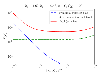
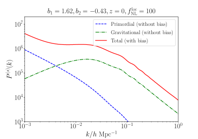
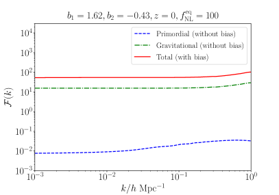
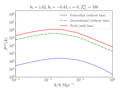
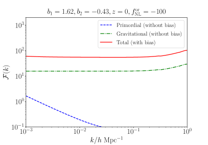
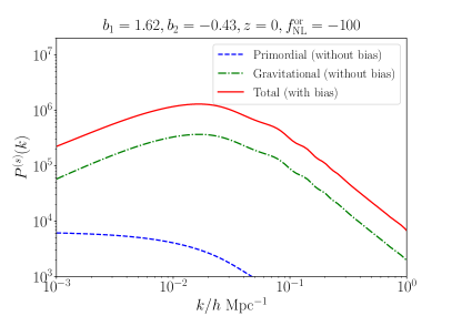
Figure 1: Left panel: The function of $\mathcal{F}(k)$ in Eq.(2.23) , for primordial non-Gaussianity for unbiased tracers at $z=0$ ($f^{\rm loc}_{\rm NL}=f^{\rm eq}_{\rm NL}=100,f^{\rm or}_{\rm NL}=-100$, blue dashed line), gravitational instability also for unbiased tracers at $z=0$ (green dotted-dashed line) and their combination for biased tracers (red solid line) with bias parameters $b_{1}=1.62,b_{2}=-0.43$, $b_{K^{2}}=0$; Right panel: Same as the left panel but for the skew spectra. The linear power spectrum adopted is that of a Planck LCDM cosmology. We also show the results for three different non-Gaussianity templates (upper: local; middle: equilateral; lower: orthogonal.)

Here $\mathcal{F}(k)$ depends weakly on cosmological parameters (via the weak dependence of the perturbation theory kernel and the transfer function), depends explicitly on bias parameters and depends linearly on the non-Gaussianity parameter $f^{\rm loc}_{\rm NL}$, which indicates how the skew spectrum carries information additional to that encoded in the the power spectrum.

The left panels of Fig. 1 shows the function of $\mathcal{F}(k)$ in Eq. (2.23) for three different non-Gaussianity templates (local, equilateral and orthogonal), gravitational instability, and their combination for biases tracers with: $f_{\rm NL}^{\rm loc}=f_{\rm NL}^{\rm eq}=100,f_{\rm NL}^{\rm or}=-100$, $z=0$ $b_{1}=1.62,b_{2}=-0.43$, $b_{K^{2}}=0$. This bias corresponds to that of halos above a minimum mass $M_{\min}=2.5\times 10^{13}h^{-1}M_{\odot}$ at $z=0$ (see Sec. 4).

For gravitational instability, $\mathcal{F}(k)$ is almost a constant on linear scales. This is not unexpected. To understand this in a simple way let us consider unbiased tracers. In this case, the function of $\mathcal{F}(k)$ for gravitational instability is,

$$\mathcal{F}(k)=2\int_{-1}^{1}d\mu\int\frac{d{q}}{(2\pi)^{2}}q^{2}\left[F_{2}(\bm{k},\bm{q})P_{g,L}(q)+F_{2}(\bm{k},\bm{\alpha})P_{g,L}(\alpha)+F_{2}(\bm{q},\bm{\alpha})\frac{P_{g,L}(q)P_{g,L}(\alpha)}{P_{g,L}(k)}\right],$$ (2.28)

if $\bm{k}\rightarrow 0$, $\bm{q}\simeq-\bm{\alpha}$, so $F_{2}(\bm{q},\bm{\alpha})=0$. We can simplify the function as,

$$\mathcal{F}(k)|_{k\rightarrow 0} = 4\int_{-1}^{1}d\mu\int\frac{d{q}}{(2\pi)^{2}}q^{2}F_{2}(\bm{k},\bm{q})P_{g,L}(q)$$ (2.29)

$$= 4\int_{-1}^{1}d\mu\int\frac{d{q}}{(2\pi)^{2}}q^{2}\left(\frac{5}{7}+\frac{2}{7}\mu^{2}\right)P_{g,L}(q)+4\int_{-1}^{1}d\mu\int\frac{d{q}}{(2\pi)^{2}}q^{2}\left[\frac{\mu}{2}\left(\frac{k}{q}+\frac{q}{k}\right)\right]P_{g,L}(q).$$ (2.30)

The first term is independent of $k$ and the second term goes to 0 because $\int_{-1}^{1}d\mu C(k)\mu=0$. Then it is proved that for gravitational instability, $\mathcal{F}(k)$ is almost a constant on large scales.

Primordial non-Gaussianity affects mostly large scales, $k<0.03~{}h\rm Mpc^{-1}$. The corresponding skew spectra (primordial non-Gaussianity, gravitational instability for unbiased tracers and their combination for biased tracers) are shown in the right panel of Fig. 1, also with $f_{\rm NL}^{\rm loc}=f_{\rm NL}^{\rm eq}=100,f_{\rm NL}^{\rm or}=-100,z=0,b_{1}=1.62,b_{2}=-0.43$, $b_{K^{2}}=0$. We find the local type non-Gaussianity has the most prominent effect at large scales, and the gravitational part becomes important at smaller scales. For the same value of the $f_{\rm NL}$ parameter, the other two templates only have a much weaker impact on the final skew spectra.

2.4.1 Comparison with other approaches to access the bispectrum information via the power spectrum

Another approach proposed to access bispectrum information via a suitable power spectrum is the “integrated bispectrum” proposed by Ref. [19], which measures an integral of the bispectrum which is dominated by the squeezed configurations.

This statistics is obtained by dividing the survey volume $V$ into $N_{s}$ subvolumes. In each sub volume, the local power spectrum (the so-called position-dependent power spectrum, $P(\bm{k},\bm{r_{L}})$) and local mean over-density , $\bar{\delta}_{r_{L}}$, are computed. Then correlating the position-dependent power spectrum with the local mean over density one obtains the so-called integrated bispectrum.

$$\left\langle P\left(\bm{k},\bm{r}_{L}\right)\bar{\delta}\left(\bm{r}_{L}\right)\right\rangle= \frac{1}{V_{L}^{2}}\int\frac{d^{3}\bm{q}_{1}}{(2\pi)^{3}}\int\frac{d^{3}\bm{q}_{3}}{(2\pi)^{3}}B_{m}\left(\bm{k}-\bm{q}_{1},-\bm{k}+\bm{q}_{1}+\bm{q}_{3},-\mathbf{q}_{3}\right)$$ (2.31)

$$\times W_{L}\left(\bm{q}_{1}\right)W_{L}\left(-\bm{q}_{1}-\bm{q}_{3}\right)W_{L}\left(\bm{q}_{3}\right),$$

where $V_{L}=V/N_{s}$, $\bm{r}_{L}$ is the center of the subvolume and $W_{L}$ are the window functions.

Because of the window functions, most of the contribution to the integrated bispectrum thus comes from values of $q_{1}$ and $q_{3}$ until approximately $1/\sqrt[3]{V_{L}}$. Ref. [19] pointed out that, if the wavenumber $\bm{k}$ is much larger than $1/\sqrt[3]{V_{L}}$, then the dominant contribution to the integrated bispectrum comes from the bispectrum in squeezed configurations, $B\left(\bm{k}-\bm{q}_{1},-\bm{k}+\bm{q}_{1}+\bm{q}_{3},-\bm{q}_{3}\right)\rightarrow B\left(\bm{k},-\bm{k},-\bm{q}_{3}\right)$ with $q_{1}\ll k$ and $q_{3}\ll k$. The integrated bispectrum becomes,

$$\left\langle P\left(\bm{k},\bm{r}_{L}\right)\bar{\delta}\left(\bm{r}_{L}\right)\right\rangle\simeq\frac{1}{V_{L}^{2}}\int^{1/\sqrt[3]{V_{L}}}\frac{d^{3}\bm{q}_{3}}{(2\pi)^{3}}B\left({k},{k},{q}_{3}\right).$$ (2.32)

By comparing this expression with the skew spectrum

$$P^{(s)}(k)=\int\frac{d^{3}\bm{q}}{(2\pi)^{3}}B(k,q,|\bm{q}-\bm{k}|),$$ (2.33)

we can appreciate that the two quantities are highly complementary; the integrated bispectrum is mostly sensitive to squeezed configurations while the skew spectrum is sensitive to a combination of all shapes. However, in the limit where $q_{3}<1/\sqrt[3]{V_{L}}$ and $k\gg q_{3}$ (i.e., $q_{3}\longrightarrow 0$) in Eq. (2.32) the skew spectrum is equivalent to the integrated bispectrum proposed by Ref. [19] for $k\longrightarrow 0$ in Eq. (2.33).

2.5 Smoothing

When comparing our theoretical predictions for the skew spectrum to data or $N$-body simulations, we should consider that the evolved field is likely highly non-linear. Our derived expression is valid on quasi-linear scales, and is expected to fail in the non-linear regime. There are several fitting formulae for the dark matter bispectrum we can use to derive a more reliable expression for the skew spectrum [39, 40]. However these formulae are only calibrated (and valid) in a specific $k$ range. To avoid this problem, we apply a smoothing filter to the field to suppress the small scales non-linear modes.

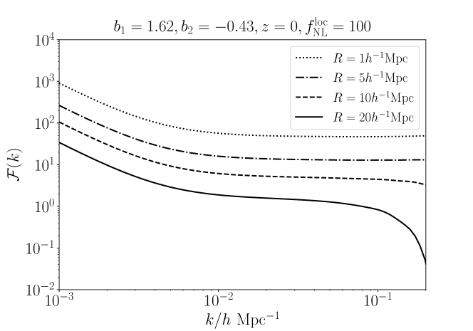
Figure 2: $\mathcal{F}(k)$ for different smoothing radii, from top to bottom: $R=1,5,10,20h^{-1}\rm Mpc$

By doing this, we may loose some information from the skew spectrum, but we can have analytical control. In this paper, we use a top-hat windows function whose Fourier transform is,

$$W_{R}(k)=\frac{3\sin(kR)}{k^{3}R^{3}}-\frac{3\cos(kR)}{k^{2}R^{2}}.$$ (2.34)

The smoothed skew spectrum becomes

$$P_{R}^{(s)}(k) = \int\frac{d^{3}\bm{q}}{(2\pi)^{3}}B(k,q,\alpha)W_{R}(k)W_{R}(q)W_{R}(\alpha).$$ (2.35)

In Fig. 2 we show ${\cal F}(k)$ with $f_{\rm NL}^{\rm loc}=100,z=0,b_{1}=1.62,b_{2}=-0.43$, for different smoothing radii. The introduction of a smoothing filter reduces the amplitude of ${\cal F}(k)$ and therefore also of $P^{(s)}(k)$. In Sec. 3 we compare the analytic expression for the skew spectrum to the measurements from $N$-body simulations.

2.6 Redshift space distortions

In this section, we extent our theory by including the RSD effect which is caused by the peculiar velocities of galaxies in the redshift measurements of surveys. This distortion depends on the growth rate of structures, and therefore in principle it can offer complementary information.

At tree-level, the galaxy bispectrum with local primordial non-Gaussianity can be conveniently written as [44, 45, 46]

$$B^{\rm RSD}_{g}(k_{1},k_{2},k_{3})=2Z_{2}\left(\bm{k}_{1},\bm{k}_{2}\right)Z_{1}\left(\bm{k}_{1}\right)Z_{1}\left(\bm{k}_{2}\right)P_{m,L}\left(k_{1}\right)P_{m,L}\left(k_{2}\right)+\mathrm{cyc.}$$ (2.36)

where the kernels $Z_{i}$ are defined as

$$Z_{1}(\bm{k}_{i})\equiv(b_{1}+f\nu_{i}^{2})$$ (2.37)

$$Z_{2}(\bm{k}_{1},\bm{k}_{2}) \equiv b_{1}\left[F_{2}\left(\bm{k}_{1},\bm{k}_{2}\right)+\frac{f\nu k}{2}\left(\frac{\nu_{1}}{k_{1}}+\frac{\nu_{2}}{k_{2}}\right)+f^{\rm loc}_{\rm NL}\frac{M(k_{3})}{M(k_{1})M(k_{2})}\right]+$$ (2.38)

$$f\nu^{2}\left[G_{2}\left(\bm{k}_{1},\bm{k}_{2}\right)+f^{\rm loc}_{\rm NL}\frac{M(k_{3})}{M(k_{1})M(k_{2})}\right]+\frac{f^{2}\nu k}{2}\nu_{1}\nu_{2}\left(\frac{\nu_{2}}{k_{1}}+\frac{\nu_{1}}{k_{2}}\right)+\frac{b_{2}}{2}~{},$$

where $f$ is the logarithmic growth rate ${\rm d}\ln\delta/{\rm d}\ln a$, $\nu_{i}$ denote the cosine of the angle between $\bm{k}_{i}$ and the line of sight, $\nu\equiv\left(\nu_{1}k_{1}+\nu_{2}k_{2}\right)/k$ and $k^{2}=\left(\bm{k}_{1}+\bm{k}_{2}\right)^{2}$. $G_{2}(\bm{k}_{1},\bm{k}_{2})$ is the second-order kernels of the velocities,

$$G_{2}\left(\bm{k}_{1},\bm{k}_{2}\right)=\frac{3}{7}+\frac{x}{2}\left(\frac{k_{1}}{k_{2}}+\frac{k_{2}}{k_{1}}\right)+\frac{4}{7}x^{2}$$ (2.39)

with $x\equiv{\bm{k}}_{1}\cdot{\bm{k}}_{2}/k_{1}k_{2}$. While the anisotropic signal of redshift space distortions for the power spectrum have been studied extensively, for the bispectrum only the angle-averaged (monopole) signal has been measured (see [47]). A closed expression for the bispectrum monopole can only be obtained for large scales where the non-linear Fingers-of-God (FoG) effect is small. This is indeed the case in the regime we are interested in. Here we model the bispectrum monopole as

$$B^{(0)}_{g}(k_{1},k_{2},k_{3}) = b_{1}^{4}\left\{\frac{1}{b_{1}}\left[F_{2}\left(\bm{k}_{1},\bm{k}_{2}\right)+f^{\rm loc}_{\rm NL}\frac{M(k_{3})}{M(k_{1})M(k_{2})}\right]\mathcal{D}_{\mathrm{SQ}1}^{(0)}+\frac{1}{b_{1}}\left[G_{2}\left(\bm{k}_{1},\bm{k}_{2}\right)+f^{\rm loc}_{\rm NL}\frac{M(k_{3})}{M(k_{1})M(k_{2})}\right]\mathcal{D}_{\mathrm{SQ}2}^{(0)}\right.$$ (2.40)

$$\left.+\frac{b_{2}}{b_{1}^{2}}\mathcal{D}_{\rm NLB}^{(0)}+\mathcal{D}_{\rm FoG}^{(0)}\right\}P_{m,L}(k_{1})P_{m,L}(k_{2})+\rm cyc.$$

where the terms $\mathcal{D}_{\mathrm{SQ}1}^{(0)}$ and $\mathcal{D}_{\mathrm{SQ}2}^{(0)}$ represent the linear and non-linear contributions to the large-scale squashing, $\mathcal{D}_{\rm NLB}^{(0)}$ is due to the non-linear biasing and $\mathcal{D}_{\rm FoG}^{(0)}$ describes (partially) the effect of damping due the Fingers of God. These terms are defined in [44].

Finally, we can write the smoothed galaxy skew spectrum monopole in redshift space as

$$P_{g}^{(s,0)}(k)=\int\frac{d^{3}\bm{q}}{(2\pi)^{3}}B_{g}^{(0)}(k,q,\alpha)W_{R}(k)W_{R}(q)W_{R}(\alpha).$$ (2.41)

The monopole redshift space power spectrum is described by

$$P_{g}^{0}(k)=\left[1+\frac{2}{3}\frac{f}{b_{1}}+\frac{1}{5}\left(\frac{f}{b_{1}}\right)^{2}\right]P_{g,L}(k)$$ (2.42)

where we also neglect the non-linear Fingers of God effects.

Of course it would not make sense to consider the real-world complications due to redshift space distortions, if the answer to the question posed in the title was ”nothing” or “very little” even in real space. For this reason we will first present real-space results and then generalise them to redshift space. This generalisation comes with a caveat: here we only consider the monopole signal (and large, linear scales), adding higher order multipoles such as the quadrupole might change quantitatively the results. But this is left for future work.

3 Simulations

We use 1000 realizations from the Quijote simulations suite [48]. The simulation’s cosmological parameters are $\Omega_{\rm m}=0.3175,\Omega_{\rm b}=0.049,h=0.6711,n_{s}=0.9624,\sigma_{8}=0.834,M_{\nu}=0.0~{}{\rm eV}$, and $f_{\rm NL}^{\rm loc}=0$, which are the matter and baryon density parameters, reduced Hubble constant, spectral index of primordial power law power spectrum, amplitude of perturbations parameter, total neutrino mass and amplitude of primordial non-Gaussianity respectively. All the simulations were run using the TreePM code Gadget-III, an improved version of Gadget-II [49]. Each realization has $512^{3}$ cold dark matter particles in a box with cosmological volume of 1$(h^{-1}\rm Gpc)^{3}$. We use the halo catalogues where halos were identified using the Friends-of-Friends algorithm [50] with linking length $b=0.2$ at $z=0$, and we set the minimal halo mass $M_{\min}=2.5\times 10^{13}h^{-1}M_{\odot}$. Details of the simulations can be found in [48].

These simulations have Gaussian initial conditions. Below we will explore forecasted error-bars also for local non-Gaussianity parameter $f^{\rm loc}_{\rm NL}$. Since the simulations have $f^{\rm loc}_{\rm NL}=0$ the resulting errors should be considered valid for a null-test hypothesis. In case of a significant detection of non-zero $f^{\rm loc}_{\rm NL}$ error-bars are expected to be different.

To calculate the skew spectra from simulations, we square the (smoothed) halo density field and treat it as a new field $\delta^{2}_{h}(\bm{x})$, then calculate the cross power spectrum with $\delta_{h}(\bm{x})$ using the routine provided in Pylians . When considering smoothing, we apply a top-hat smoothing filter with $R=20h^{-1}\rm Mpc$ before squaring the density field. With this smoothing choice we find that standard perturbation theory is sufficient to describe the skew spectra. This smoothing filter also ensures that in redshift space, non-linear Fingers-of-God effects are negligible.

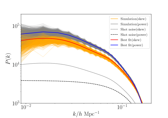
Figure 3: Power spectra (grey lines) and skew spectra (orange lines) from 1000 simulations, the black dotted line and dashed line are shot noise for skew spectrum and power spectrum, respectively. Solid lines correspond to the best-fit theoretical models (details can be found in Sec. 4). The smoothing radius is $R=20h^{-1}\rm Mpc$

3.1 Shot noise

Both power spectrum and skew spectrum of the halo density have an additional stochasticity contribution (shot noise) whose Poissonian predictions are [23]

$$P_{h,{\rm measured}}(k)=P_{h}(k)+P_{h,\rm shot}(k)\,;\,\,\,P_{h,\rm shot}(k)=\frac{1}{n_{h}},$$ (3.1)

and for the skew spectrum,

$$P^{(s)}_{h,\rm shot}(k)=\int\frac{d^{3}\bm{q}}{(2\pi)^{3}}\left[\frac{1}{n_{h}}\left(P_{h}(k)+P_{h}(q)+P_{h}(|\bm{q}-\bm{k}|)\right)+\frac{1}{n_{h}^{2}}\right],$$ (3.2)

where $n_{h}$ is the halo number density and $P_{h}(k)$ is the halo power spectrum with shot noise subtracted. Because of halo-exclusion e.g., [51, 52], we cannot expect the shot noise contribution to be exactly Poissonian. Following Ref. [45], who used a simple, 1-free parameter model for the halo shot noise, and found the shot noise for a halo population to be slight sub-Poisson, we adopt the following parameterizations,

$$P_{h,\rm shot}(k)=(1-A_{\rm noise})\frac{1}{n_{h}},$$ (3.3)

$$P^{(s)}_{h,\rm shot}(k)=(1-A_{\rm noise})\int\frac{d^{3}\bm{q}}{(2\pi)^{3}}\left[\frac{1}{n_{h}}\left(P_{h}(k)+P_{h}(q)+P_{h}(|\bm{q}-\bm{k}|)-\frac{3A_{\rm noise}}{n_{h}}\right)+\frac{1}{n_{h}^{2}}\right],$$ (3.4)

here $A_{\rm noise}$ is a free parameter to account for deviations from Poisson behaviour. Neither from BOSS data [15] nor from the simulations we use here there is evidence for the $A_{\rm noise}$ phenomenological shot noise correction to take different values for the power spectrum and the bispectrum or for the the power spectrum (Eq. (3.3)) and the skew spectrum (Eq. (3.4)). Here we therefore adopt only one $A_{\rm noise}$ parameter for both statistics. While this assumption may not hold in detail for future data, it is not expected to change the conclusions of this work. Since in practice a good prior on $A_{\rm noise}$ may be obtained e.g., from scale smaller than those considered here. We present our main results by fixing $A_{\rm noise}$ in the joint analysis to its best fit value obtained for a fixed (underling) cosmology. We then also show how results change when $A_{\rm noise}$ is allowed to float along with all the other parameters. We anticipate here that the first approach is slightly more conservative: including the skew spectrum give in this case slightly smaller gains (see also appendix B).

In Fig. 3 we plot the real-space power spectra (gray) and skew spectra (orange) obtained from the $z=0$ smoothed halo field (for halos above $M_{\min}=2.5\times 10^{13}h^{-1}M_{\odot}$) of the simulations and their corresponding shot noise. Each of the thin lines correspond to one simulation. The thick blue and red lines are our theoretical predictions for the best-fit parameters in particular for bias and shot noise which are $A_{\rm noise}=0.22,b_{1}=1.635,b_{2}=-0.426$. These values of the linear bias and of $A_{\rm noise}$ coincide with those obtained by fitting the ratio of the power spectra of the halos and of the dark matter at scales $k<0.1$ $h$/Mpc (see details in Sec. 4).

The skew spectra from simulations in Fig. 3 are smaller than the theory prediction (right panel of Fig. 1), because here we use a smoothing filter and the contribution from smaller scales is suppressed.

The corresponding plots in redshift space (monopole) are qualitatively very similar reported in appendix C.

3.2 Covariances

Before being able to perform a joint analysis of power spectrum and skew spectrum, we need to evaluate the full covariance of both of these two quantities. We estimate it from the Quijote simulations using a wavenumber range $k=[0.0089,0.1]h\rm Mpc^{-1}$, in 15 $k$ bins uniformly spaced in log $k$. We start by combining $P_{h}(k)$ and $P_{h}^{(s)}(k)$ into a “data” vector $P^{(p+s)}_{h}(K_{i})$ ($i=1,\ldots,15$ for the power spectrum and $i=16,\ldots,30$ for the skew spectrum).

In the left panel of Fig. 4 we plot the correlation matrix of $P^{(p+s)}_{h}(K_{i})$, defined as

$$\frac{C^{*}_{K_{i},K_{j}}}{\sqrt{C^{*}_{K_{i},K_{i}}C^{*}_{K_{j},K_{j}}}},$$ (3.5)

where $C^{*}_{K_{i},K_{j}}$ is the estimated covariance of $P^{(p+s)}_{h}(K_{i})$. As expected from Eq.(2.23), skew spectrum and power spectrum are highly coupled at the same $k$-mode. However in the linear-quasi-linear regime of interest here different $k$ modes are very weakly correlated.

Ref. [53] pointed that the inverse of the maximum-likelihood estimator of the covariance matrix is a biased estimator of the inverse population covariance matrix, and this bias depends on the ratio of the dimensionality of the matrix $p$ to the number of independent observations $n$. This bias can be corrected by introducing a Hartlap factor [53],

$$C^{-1}=\frac{n-p-2}{n-1}(C^{*})^{-1}.$$ (3.6)

In our analysis, $n=1000$ and $p=30$, which only leads to a percent level correlation which we include.

In the right panel of Fig. 4, we also show the relative error on the power spectrum $\Delta P_{h}(k)/\bar{P_{h}}(k)$ obtained from the simulations and the theory prediction,

$$\Delta P_{h}(k)/\bar{P_{h}}(k)=\frac{\sqrt{(2\pi)}}{\sqrt[3]{V}k}$$ (3.7)

where $V$ is the simulation volume. From the residuals we can appreciate that this estimation is unbiased. The errors are large at large scales due to cosmic variance.

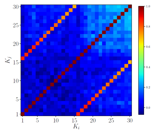
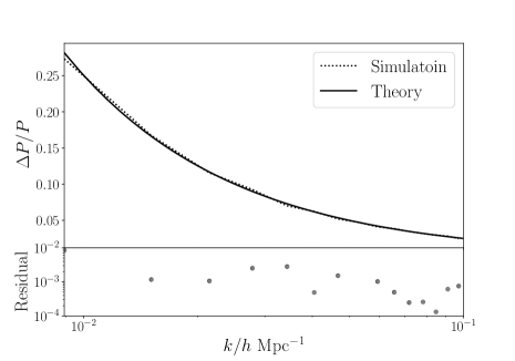
Figure 4: Left panel: the correlation matrix of $P^{(p+s)}_{h}(K_{i})$ defined in Eq.(3.5); Upper right panel: $\Delta P(k)/\bar{P}(k)$ for power spectrum from simulations (dotted line) and theory prediction (solid line); Lower right panel: corresponding residuals (in absolute value).

3.3 Fitting procedure and error estimate

We next consider one of the 1000 realisations as our “mock” Universe to try to constrain its cosmological parameters by fitting the power spectrum and skew spectrum; maximum and minimum scales are: $k_{\min}=0.0089~{}h\rm Mpc^{-1}$ and $k_{\max}=0.1~{}h\rm Mpc^{-1}$, respectively. Here we only consider the tree-level model of the power spectrum since we find that it is sufficient for our purposes in the range of scales considered (i.e. adding higher order corrections does not change the final results). This can be understood by considering non only that one loop corrections are small, but also that the covariance is obtained directly from simulations and we are only interested in the relative errors (i.e., with/without skew spectrum).

We modified the public software CosmoMC [54], a Markov Chain Monte Carlo (MCMC) code to calculate the skew spectrum and perform joint Bayesian parameter inference. A simple $\chi^{2}$ is used for parameter fitting in our analysis:

$$\chi^{2}=\left[\hat{P}_{h}^{(p+s)}(K_{i})-P^{(p+s)}(K_{i})\right]C^{-1}_{K_{i},K_{j}}\left[\hat{P}_{h}^{(p+s)}(K_{j})-P^{(p+s)}(K_{j})\right]^{T},$$ (3.8)

where $\hat{P}_{h}^{(p+s)}$ and $P_{h}^{(p+s)}$ represent the model and the measured spectra. We recognise that in principle one should use a more appropriate likelihood, the adopted procedure would be correct only if the data vector has a Gaussian distribution which covariance matrix does not depend on the parameters to be estimated. It is well known that the power spectrum does not follow a Gaussian distribution, however the adoption of Eq.(3.8) is a good approximation especially for well populated bandpowers see. e.g., [55] and Refs. therein. The distribution for the skew spectrum is certainly non-Gaussian so the adoption of Eq.(3.8) is not a priori justified, but we expect it would be valid with the central limit theorem. Here, we adopt Eq.(3.8) as our ansatz and we will assess its performance and show it is a sufficiently good approximation below.

Thus, with this in mind, the best-fit parameters are obtained by finding the minimal of $\chi^{2}$, and the confidence regions are then defined by the surfaces of constant $\Delta\chi^{2}=\chi^{2}-\chi_{\min}^{2}$, where $\chi_{\min}^{2}$ is the minimal value of $\chi^{2}$ and $\Delta\chi^{2}$ are functions of the number of parameters for the joint confidence levels.

We then repeat the fitting process for the other 999 simulations only to find their best-fit parameter values. By doing this, we can check that the scatter of recovered parameters among the simulations is consistent with the confidence contours given by the MCMC-based inference. This is the test that supports our adoption of Eq.(3.8).

4 Results

We start by determining the shot noise correction term and the bias parameters $\{A_{\rm noise},b_{1},b_{2}\}$ simultaneously with the fiducial cosmology fixed. Results are shown in Fig. 5 and Tab. 1.

We find that $b_{1}=1.635\pm 0.028$, $b_{2}=-0.426\pm 0.081$ and $A_{\rm noise}=0.22\pm 0.15$ (1$\sigma$ C.L.) which shows a slight sub-Poisson shot noise. The relationship between $b_{1}$ and $b_{2}$ is also consistent with expectations for the selected halos [56, 41]. We find no difference when adopting $b_{K^{2}}=0$ or $b_{K^{2}}=-4/7(b_{1}-1)$, this is further discussed in appendix A. To check consistency, we calculate the best-fit results of $b_{1}$ and $A_{\rm noise}$ using a direct measurement from the ratio of the halo power spectra and the dark matter power spectra at scales $0.0089<k<0.1$ $h$/Mpc. Using 1000 Quijote realizations, the fitting results of $b_{1}$ and $A_{\rm noise}$ are $b_{1}=1.629\pm 0.021$ and $A_{\rm noise}=0.183\pm 0.114$ ($1\sigma$ C.L.), which confirms our adopted values. The same analysis repeated in redshift space show fully consistent results, see appendix C.

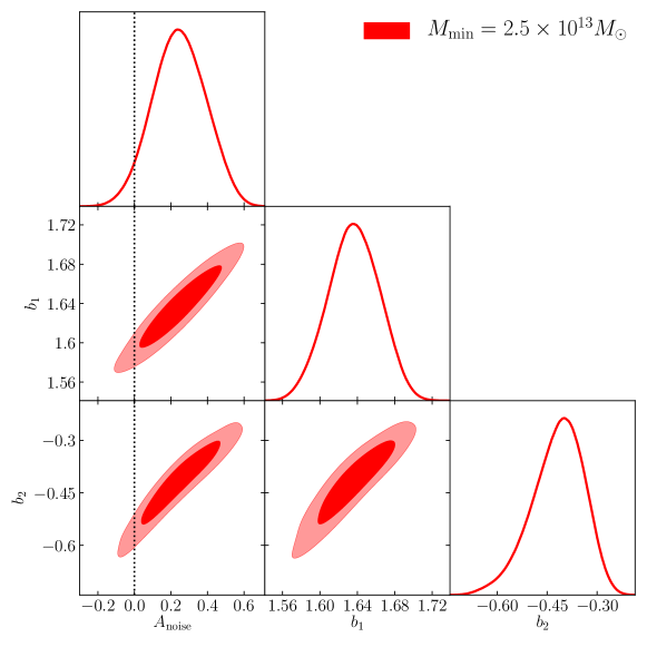
Figure 5: Marginalized two-dimensional distributions (1$\sigma$ and 2$\sigma$ contours) and posterior distributions for $A_{\rm noise}$, $b_{1}$ and $b_{2}$. This run is used only to set $A_{\rm noise}$.

Table 1: The best-fit results of $A_{\rm noise}$, $b_{1}$ and $b_{2}$ and their (marginalized, 1$\sigma$) errors. This run is used only to set $A_{\rm noise}$.

$b_{1}$	$b_{2}$	$A_{\rm noise}$
$1.635\pm 0.028$	$-0.426\pm 0.081$	$0.22\pm 0.15$

Now we fix $A_{\rm noise}$ at the best-fit value, and proceed to investigate the potential offered by the combination of power spectrum and skew spectrum. This is motivated by the fact that in a real application the shot noise and its correction can be determined much more accurately than we can do here by using for example non-linear scales (where the shot noise dominates).

In this paper we mainly focus on 5 parameters $\{A_{s},n_{s},f_{\rm NL}^{\rm loc},b_{1},b_{2}\}$, where $A_{s}$ and $n_{s}$ are the amplitude and spectral index of the primordial spectrum. The other cosmological parameters have been fixed at their fiducial values. It is worth mentioning that the Quijote simulations do not include primordial non-Gaussianity, hence we should recover $f_{\rm NL}^{\rm loc}=0$ within error bars. While the primordial non-Gaussianity contribution to the skew spectrum is shown in Eq.(2.10), the halo power spectrum can be greatly affected by relatively small values of $f_{\rm NL}^{\rm loc}$ via the non-Gaussian large-scale bias [57, 58, 59, 60, 30, 61, 62],

$$\frac{\Delta b_{1}}{b_{1}-1}=2f_{\rm NL}^{\rm loc}\frac{\delta_{c}}{M(k,z)W_{R}(k)}q~{},$$ (4.1)

where $\delta_{c}\simeq 1.686$ is the threshold for collapse and the correction $q=0.75$ is calibrated from $N$-body simulations [58].

In Fig. 6 we show the marginalized 2-D contours for all the parameters using the power spectrum alone and the combination of power spectrum and skew spectrum. We can see $A_{s},b_{1},b_{2}$ are highly correlated and show a very strong degeneracy. Therefore we construct a new variable $10^{9}\times b_{1}^{2}A_{s}$ to quantify the extra information the skew spectrum can give us. From the results, we find the constraints are consistent with the fiducial values, indicating that the procedure is not biased. As expected, adding the skew spectrum results in tighter constraints. For a more quantitative estimate of the constraining power of the skew spectrum, we list the best-fit values and their marginalized $1\sigma$ errors in Tab. 2. The addition of the skew spectrum to the power spectrum yields a reduction of the errors by $31\%,22\%,44\%$ for $b_{1}^{2}A_{s},n_{s}$ and $f_{\rm NL}^{\rm loc}$ respectively. The constraints on $b_{1}$ and $A_{s}$ are unrepresentative since they are strongly degenerate.

The figure also shows the scatter of the best-fit results (power spectrum and skew spectrum combined) of the 1000 realisations is consistent with the confidence contours obtained by the MCMC-based inference. This indicates that our ansatz for the likelihood in Eq.(3.8) is sufficiently accurate for this application for the joint analysis (perhaps not unexpectedly it is not too good for poorly constrained parameters which enter only in the skew spectrum). We find that if $A_{\rm noise}$ is allowed to vary as a nuisance parameter, along with the other cosmological parameters, the resulting cosmological constraints are weaker, but the gain arising from adding the skewed spectrum to the power spectrum is greater. In particular we find that $1\sigma$ marginalized errors for $b_{1}A_{s},n_{s},f_{\rm NL}^{\rm loc}$ are reduced by $44\%,39\%,47\%$ by including the skew spectrum. Details are in appendix B.

We repeated the analysis on redshift space for the power spectrum and skew spectrum monopole and find that by combining the skew spectrum to the power spectrum the 1-$\sigma$ marginalized errors $b^{2}A_{s}$, $n_{s}$ and $f^{\rm loc}_{\rm NL}$ are reduced by 41%, 26%, 39% respectively for fixed $A_{\rm noise}$. The details are reported in Appendix C.

The error reduction provided by the inclusion of the skew spectrum can be understood as follows. Eq.(2.23) and Eq.(2.24) indicate that the (tracer) skew spectrum can be seen as a (tracer) power spectrum modulated by a scale-dependent function, whose amplitude and scale dependence depend on the key parameters with a scaling that is different from the power spectrum dependence. Hence the additional information enclosed in $\mathcal{F}(k)$ can be used to reduce degeneracies among parameters that are present at the level of the power spectrum.

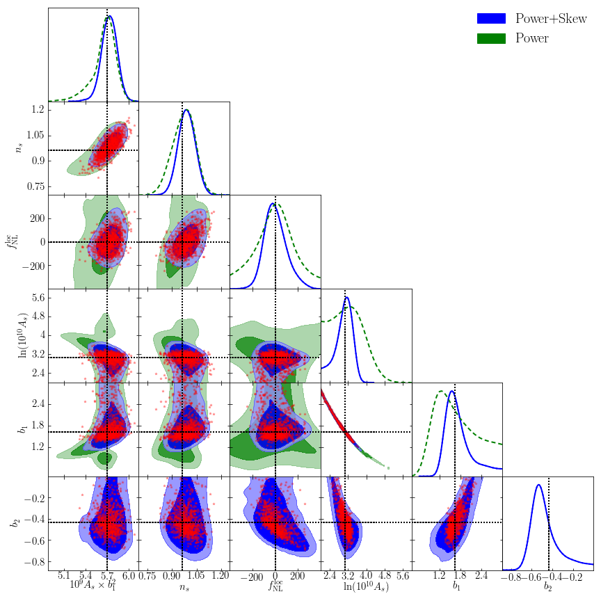
Figure 6: Marginalized two-dimensional distributions (1$\sigma$ and 2$\sigma$ contours) and posterior distributions for $10^{9}\times b_{1}^{2}A_{s},n_{s},f_{\rm NL}^{\rm loc},\ln(10^{10}A_{s}),b_{1}$ and $b_{2}$ from power spectrum only (green) and power spectrum together with skew spectrum (blue). The red stars indicate the best-fit points from 1000 simulations using power spectrum and skew spectrum, and black dotted lines are their input values used in the Quijote simulations.

Table 2: The best-fit results of $10^{9}\times b_{1}^{2}A_{s},n_{s}$ and $f_{\rm NL}^{\rm loc}$, together with their marginalized 1$\sigma$ errors.

Parameters	Power spectrum	Power + skew spectrum
$10^{9}\times b_{1}^{2}A_{s}$	$5.661\pm 0.163$	$5.714\pm 0.112$
$n_{s}$	$0.972\pm 0.068$	$0.983\pm 0.054$
$f_{\rm NL}^{\rm loc}$	$-2.9\pm 167.8$	$-8.9\pm 94.3$
$\ln(10^{10}A_{s})$	$2.37^{+0.84}_{-1.32}$	$3.31_{-0.77}^{+0.29}$
$b_{1}$	$2.29^{+0.71}_{-1.48}$	$1.45_{-0.31}^{+0.69}$
$b_{2}$	—	$-0.51^{+0.52}_{-0.41}$

5 Conclusions and discussion

In this paper, we have considered a relatively unexplored statistic, the skew spectrum, which is estimated using the cross spectrum of the squared density field $\delta^{2}(\bm{x})$ with the field $\delta(\bm{x})$ itself. Computationally, evaluation of skew spectrum is equivalent (in terms of speed and complications) to a power spectrum estimation, but the skew spectrum contains 3-point clustering (bispectrum) information. While the use of the full bispectrum provides optimal constraints, and it is the correct approach to access all the information enclosed in the three-point function, its practical implementation is challenging. This has motivated the search for alternative statistics that can capture partial information but a much reduced cost (and improved speed). One of them is the integrated bispectrum [19], the skew spectrum is another, complementary, alternative.

We have derived the general form of skew spectrum and then considered three main contributions: the primordial non-Gaussianity, gravitational instability and galaxy (halo) bias both in real space and redshift space. Finally we expressed this specific skew spectrum as a function of a scale-dependent function, $\mathcal{F}(k)$, times power spectrum. Because of the non-linear nature of $\mathcal{F}(k)$, and its peculiar dependence on key parameters such as the bias and non-Gaussianity parameters, the skew spectrum offers an extra handle on these. We have built on the works of Refs.[22, 23, 26] who also consider the skew spectrum for primordial non-Gaussianity, bias and gravitational evolution. However here we address a different issue: we ask what can be the added value of combining skew spectrum and power spectrum in a joint analysis. This has not been addressed before in the literature, but it is a question worth asking before deciding whether to proceed to measure the skew spectrum from real galaxy surveys. Usually these type of analyses are done via a Fisher matrix approach. Here however, because of the high covariance between power spectrum and Skew spectrum, and the complex properties of the skew-spectrum covariance, we resort to numerically computed covariance from a suite of 1000 state-of-the art simulations.

We have compared both the performance of our modelling for the skew spectrum and simulation results by resorting to the Quijote suite. We find that our analytic modelling of the skew spectrum reproduce the simulations well if the cosmological density (or halo) field is smoothed on linear or quasi-linear scales. The addition of the skew spectrum to the power spectrum provides a reduction of $31\%,22\%,44\%$ on the error of the parameters $b_{1}^{2}A_{s},n_{s}$ and $f_{\rm NL}^{\rm loc}$ respectively. this gains also hold in redshift space when considering only the monopole. However, by limiting the analysis to the linear scales considered here (we adopt a top hat smoothing filter of $20$ Mpc$/h$), the skew spectrum only lift very partially the degeneracy between $A_{s}$ and the linear and quadratic bias parameters. Nevertheless a reduction of $44\%$ on the error of $f_{\rm NL}^{\rm loc}$ is interesting as it would correspond to roughly doubling the survey volume if one were to use the power spectrum only (in the same $k$-range). It is possible that with a more sophisticated modelling of the gravitational instability kernel, the analysis could be pushed to higher $k$ further lifting the remaining degeneracies.

Because of its simplicity, the use of the skew spectrum in a standard pipeline for analysis of galaxy surveys could offer a powerful and fast cross check for possible systematics errors in a joint power spectrum+bispectrum analysis. Moreover, we envision that a statistics like the skew spectrum could be used, instead of the bispectrum in a practical application to a galaxy survey along the power spectrum, if one is only interested in reducing the errors on the linear and quadratic bias parameters. In fact Ref. [23] shows that for initially gaussian fields, this statistics is (near) optimal, in the sense that if used with inverse variance weighting, it captures virtually all the information present in the angle-independent part of the bispectrum, and therefore in the combination $b_{1}^{2}b_{2}$. Here we do not use the optimal weighting, but the resulting statistics, while sub-optimal, is still unbiased. We conclude by acknowledging that while only the auto skew spectrum was considered here, in the present era of multi-tracers cosmology, the (cross) skew spectrum can be a much richer quantity. For example, given two tracers, $i$ and $j$ of the same (density) field, one could form 4 cross skew spectra $\delta_{i}^{2}$$\times$ $\delta_{j}$, $\delta_{j}^{2}\times\delta_{i}$, $\delta_{i}\delta_{j}\times\delta_{j}$, $\delta_{i}\delta_{j}\times\delta_{i}$, compared to one cross power spectrum $P_{ij}$. We envision that the combination of the (auto+cross) skew spectra to the (auto+cross) power spectra could be very synergetic, both in terms of reducing error bars on cosmological parameters and in helping to control possible systematic errors in the measurement and/or its interpretation. We leave this exploration to future work.

Appendix A Effect of $b_{K^{2}}$

Here we show that the exact value adopted for $b_{K^{2}}$ does not affect our conclusions. Fig. 7 shows that the effect on the skew spectrum (in real space) is at the 1% level. We compare results obtained for two values: $b_{K^{2}}=0$ (no shear bias, as if bias was local in Eulerian space) and $b_{K^{2}}=-4/7(b_{1}-1)$ (bias is local in Lagrangian space. This is shown in Fig. 8 for real space.

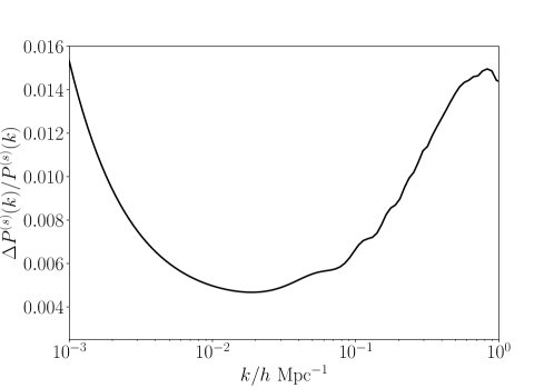
Figure 7: The relative difference in the skew spectrum induced by the tidal bias with $b_{K^{2}}=-4/7(b_{1}-1)$ where we fix $b_{1}=1.62,b_{2}=-0.43,f_{\rm NL}^{\rm loc}=0$ and the power spectrum adopted is a Planck $\Lambda$CDM model. Note that the scales adopted in this work are $k<0.1h/Mpc$.

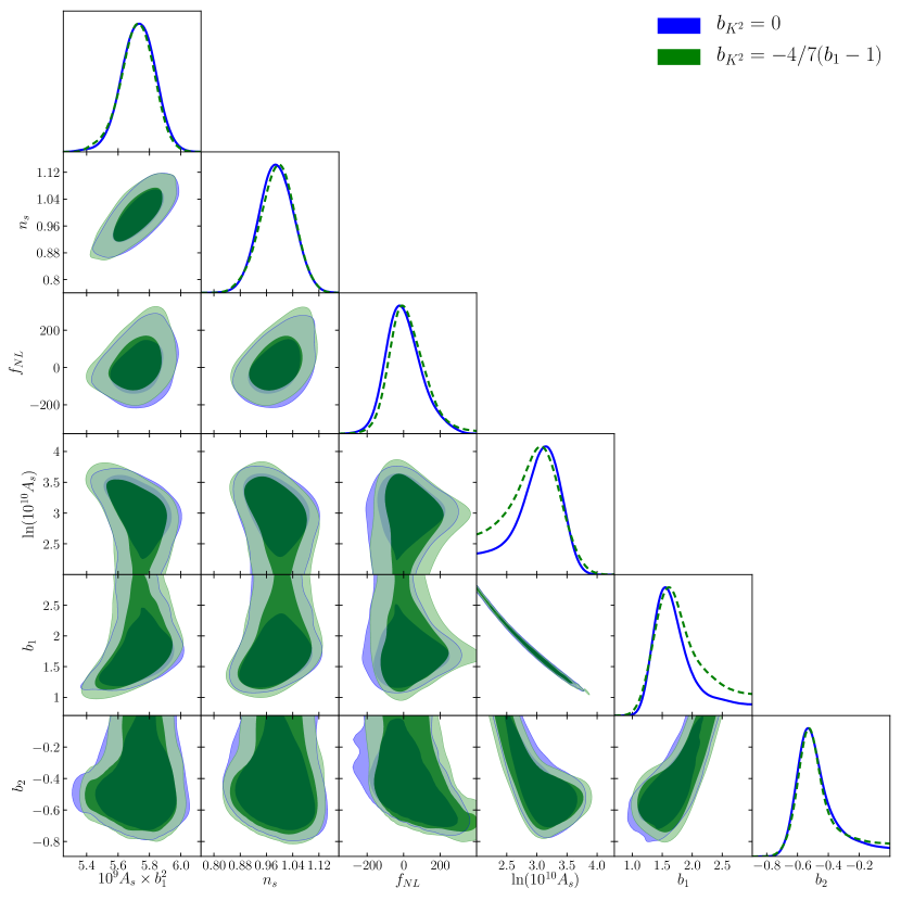
Figure 8: Effect of the adopted value for $b_{K^{2}}$. Marginalized two-dimensional distributions and posterior distributions for all the parameters of interest. We use the combination of power spectrum and skew spectrum and consider $b_{K^{2}}=-4/7(b_{1}-1)$ (green) and $b_{K^{2}}=0$ (blue, results in the main text.). This shows that our results are insensitive to the specific value of $b_{K^{2}}$ in this range.

Appendix B Effect of treating $A_{\rm noise}$ as a free parameter in the joint fit.

Here we show that, allowing $A_{\rm noise}$ to float along the other cosmological parameters in the joint fit does not invalidate our findings. On the contrary it yields slightly better forecasted improvement when adding the skew power spectrum. Fig. 9 is the analogous to Fig. 6 in the main text in real space, Fig.10 is in redshift space.

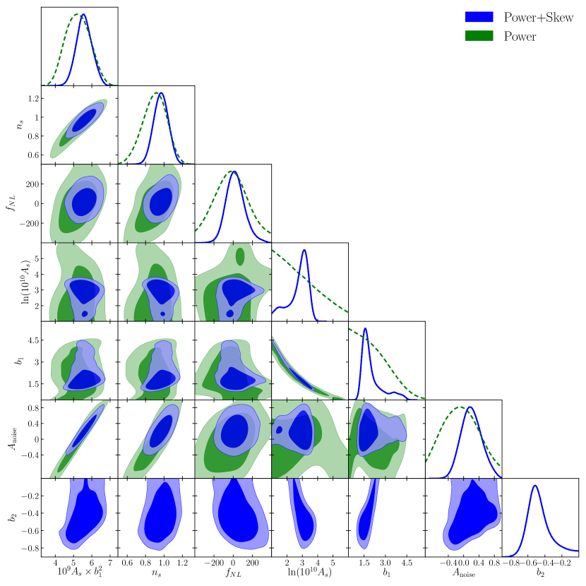
Figure 9: This is the analogous of Fig. 6 in the main text. Parameters constraints in real space, but treating $A_{\rm noise}$ as a free parameter. The conclusions to not change significantly but the errors are are larger due to the degeneracies with $A_{\rm noise}$ (especially $n_{s}$ and $b_{1}^{2}A_{s}$).

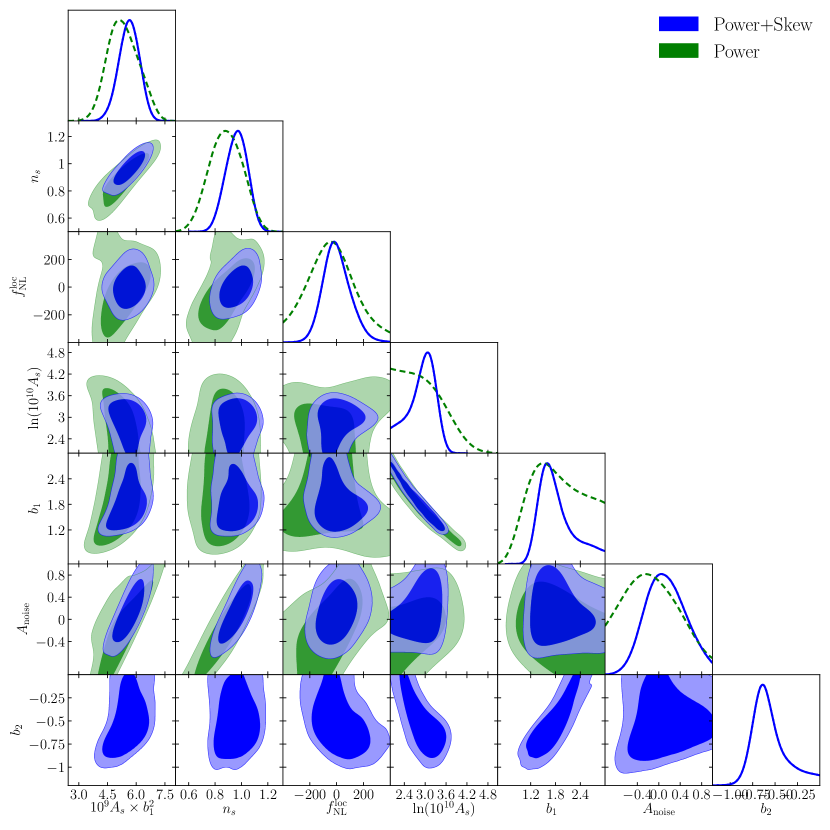
Figure 10: Same as Fig. 9 but in redshift space.

Appendix C Redshift space analysis

While we have presented real space results in the main text and discussed how the redshift space analysis yields very similar conclusions we report the details here.

In Fig. 11 and Fig. 12 we show the redshift-space fits to the skew spectrum and for the bias parameters and $A_{\rm noise}$, these figures correspond to Figs.  3 and 5 of the main text respectively. Here we use only the monopole signal. While the anisotropic signal in the power spectrum has been extensively used in the literature this is not the case for the bispectrum. For this reason for this initial investigation we limit ourselves to the monopole for both statistics. The resulting constraints on cosmological parameters of interest (also varying $A_{\rm noise}$) are shown in Fig. 10. In summary in redshift space adding skew spectrum to power spectrum the $1-\sigma$ marginalized errors for parameters $b_{2}A_{s}$, $n_{s}$ and $f_{\rm NL}^{\rm loc}$ are reduced by 41%, 26%, 39% respectively.

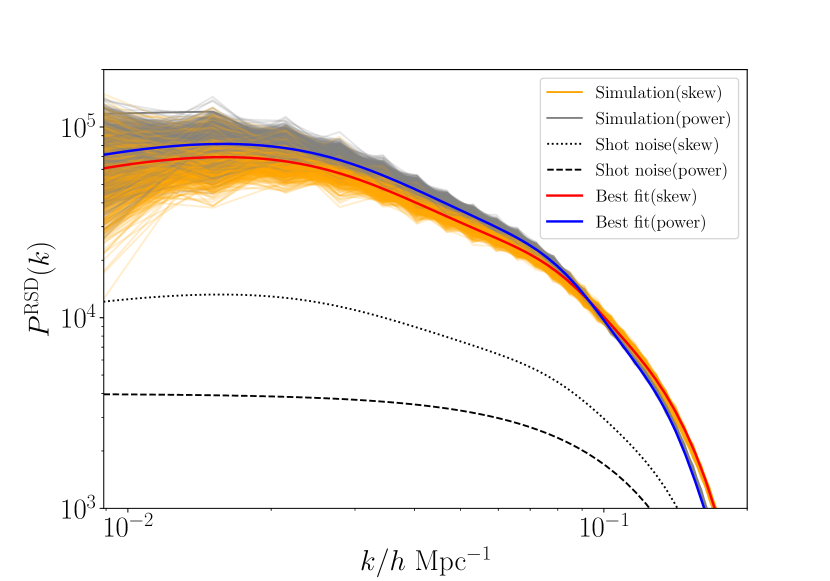
Figure 11: Same as Fig. 3 in the main text but in redshift space. The best-fit bias parameters and noise correction are: $b_{1}=1.61,b_{2}=-0.62,A_{\rm noise}=0.16$

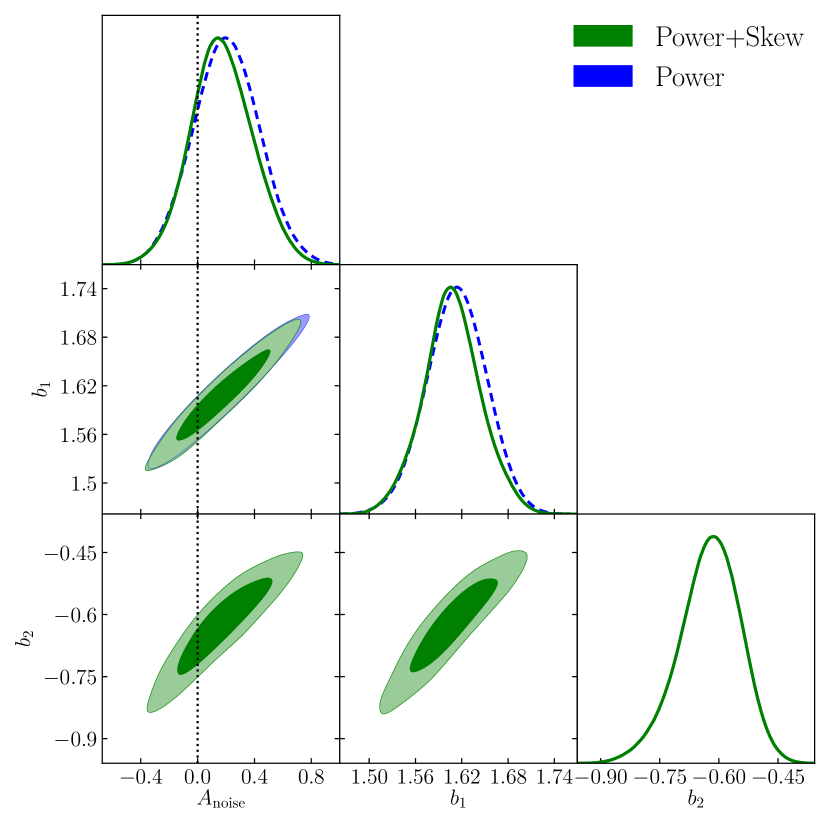
Figure 12: Same as Fig. 5 in the main text but in redshift space. When adopting the combination of power spectrum and skew spectrum, the marginalized $1\sigma$ constraints are: $b_{1}=1.606\pm 0.036,b_{2}=-0.619\pm 0.077,A_{\rm noise}=0.164\pm 0.218$, fully consistent with the real space analysis.

References

- [1] Planck collaboration, Planck 2018 results. VI. Cosmological parameters, 1807.06209.
- [2] K. Abazajian et al., CMB-S4 Science Case, Reference Design, and Project Plan, 1907.04473.
- [3] DESI collaboration, The DESI Experiment Part I: Science,Targeting, and Survey Design, 1611.00036.
- [4] L. Amendola et al., Cosmology and fundamental physics with the Euclid satellite, Living Rev. Rel. 21 (2018) 2 [1606.00180].
- [5] LSST Science, LSST Project collaboration, LSST Science Book, Version 2.0, 0912.0201.
- [6] S. Matarrese, L. Verde and A. F. Heavens, Large scale bias in the universe: Bispectrum method, Mon. Not. Roy. Astron. Soc. 290 (1997) 651 [astro-ph/9706059].
- [7] L. Verde, A. F. Heavens, S. Matarrese and L. Moscardini, Large scale bias in the universe. 2. Redshift space bispectrum, Mon. Not. Roy. Astron. Soc. 300 (1998) 747 [astro-ph/9806028].
- [8] R. Scoccimarro, The bispectrum: from theory to observations, Astrophys. J. 544 (2000) 597 [astro-ph/0004086].
- [9] E. Sefusatti, M. Crocce, S. Pueblas and R. Scoccimarro, Cosmology and the Bispectrum, Phys. Rev. D74 (2006) 023522 [astro-ph/0604505].
- [10] K. Hoffmann, J. Bel, E. Gazta aga, M. Crocce, P. Fosalba and F. J. Castander, Measuring the growth of matter fluctuations with third-order galaxy correlations, Mon. Not. Roy. Astron. Soc. 447 (2015) 1724 [1403.1259].
- [11] R. Scoccimarro, H. A. Feldman, J. N. Fry and J. A. Frieman, The Bispectrum of IRAS redshift catalogs, Astrophys. J. 546 (2001) 652 [astro-ph/0004087].
- [12] L. Verde et al., The 2dF Galaxy Redshift Survey: The Bias of galaxies and the density of the Universe, Mon. Not. Roy. Astron. Soc. 335 (2002) 432 [astro-ph/0112161].
- [13] WiggleZ collaboration, The WiggleZ Dark Energy Survey: constraining galaxy bias and cosmic growth with 3-point correlation functions, Mon. Not. Roy. Astron. Soc. 432 (2013) 2654 [1303.6644].
- [14] H. Gil-Mar n, J. Nore a, L. Verde, W. J. Percival, C. Wagner, M. Manera et al., The power spectrum and bispectrum of SDSS DR11 BOSS galaxies I. Bias and gravity, Mon. Not. Roy. Astron. Soc. 451 (2015) 539 [1407.5668].
- [15] H. Gil-Mar n, L. Verde, J. Nore a, A. J. Cuesta, L. Samushia, W. J. Percival et al., The power spectrum and bispectrum of SDSS DR11 BOSS galaxies II. Cosmological interpretation, Mon. Not. Roy. Astron. Soc. 452 (2015) 1914 [1408.0027].
- [16] H. Gil-Mar n, W. J. Percival, L. Verde, J. R. Brownstein, C.-H. Chuang, F.-S. Kitaura et al., The clustering of galaxies in the SDSS-III Baryon Oscillation Spectroscopic Survey: RSD measurement from the power spectrum and bispectrum of the DR12 BOSS galaxies, Mon. Not. Roy. Astron. Soc. 465 (2017) 1757 [1606.00439].
- [17] A. Eggemeier, R. Scoccimarro and R. E. Smith, Bias Loop Corrections to the Galaxy Bispectrum, Phys. Rev. D99 (2019) 123514 [1812.03208].
- [18] M. Colavincenzo et al., Comparing approximate methods for mock catalogues and covariance matrices III: bispectrum, Mon. Not. Roy. Astron. Soc. 482 (2019) 4883 [1806.09499].
- [19] C.-T. Chiang, C. Wagner, F. Schmidt and E. Komatsu, Position-dependent power spectrum of the large-scale structure: a novel method to measure the squeezed-limit bispectrum, JCAP 1405 (2014) 048 [1403.3411].
- [20] A. Cooray, Squared temperature-temperature power spectrum as a probe of the CMB bispectrum, Phys. Rev. D64 (2001) 043516 [astro-ph/0105415].
- [21] D. Munshi and A. Heavens, A New Approach to Probing Primordial Non-Gaussianity, Mon. Not. Roy. Astron. Soc. 401 (2010) 2406 [0904.4478].
- [22] G. Pratten and D. Munshi, Non-Gaussianity in Large Scale Structure and Minkowski Functionals, Mon. Not. Roy. Astron. Soc. 423 (2012) 3209 [1108.1985].
- [23] M. Schmittfull, T. Baldauf and U. Seljak, Near optimal bispectrum estimators for large-scale structure, Phys. Rev. D91 (2015) 043530 [1411.6595].
- [24] K. C. Chan and L. Blot, Assessment of the Information Content of the Power Spectrum and Bispectrum, Phys. Rev. D96 (2017) 023528 [1610.06585].
- [25] D. Munshi and P. Coles, The Integrated Bispectrum and Beyond, JCAP 1702 (2017) 010 [1608.04345].
- [26] A. Moradinezhad Dizgah, H. Lee, M. Schmittfull and C. Dvorkin, Capturing Non-Gaussianity of the Large-Scale Structure with Weighted Skew-Spectra, 1911.05763.
- [27] F. Bernardeau, The Large scale gravitational bias from the quasilinear regime, Astron. Astrophys. 312 (1996) 11 [astro-ph/9602072].
- [28] J. E. Pollack, R. E. Smith and C. Porciani, A new method to measure galaxy bias, Mon. Not. Roy. Astron. Soc. 440 (2014) 555 [1309.0504].
- [29] C.-T. Chiang, C. Wagner, A. G. S nchez, F. Schmidt and E. Komatsu, Position-dependent correlation function from the SDSS-III Baryon Oscillation Spectroscopic Survey Data Release 10 CMASS Sample, JCAP 1509 (2015) 028 [1504.03322].
- [30] S. Matarrese and L. Verde, The effect of primordial non-Gaussianity on halo bias, Astrophys. J. 677 (2008) L77 [0801.4826].
- [31] D. S. Salopek and J. R. Bond, Nonlinear evolution of long wavelength metric fluctuations in inflationary models, Phys. Rev. D42 (1990) 3936.
- [32] A. Gangui, F. Lucchin, S. Matarrese and S. Mollerach, The Three point correlation function of the cosmic microwave background in inflationary models, Astrophys. J. 430 (1994) 447 [astro-ph/9312033].
- [33] L. Verde, R. Jimenez, M. Kamionkowski and S. Matarrese, Tests for primordial nonGaussianity, Mon. Not. Roy. Astron. Soc. 325 (2001) 412 [astro-ph/0011180].
- [34] E. Komatsu and D. N. Spergel, Acoustic signatures in the primary microwave background bispectrum, Phys. Rev. D63 (2001) 063002 [astro-ph/0005036].
- [35] D. Seery and J. E. Lidsey, Primordial non-Gaussianities in single field inflation, JCAP 0506 (2005) 003 [astro-ph/0503692].
- [36] X. Chen, M.-x. Huang, S. Kachru and G. Shiu, Observational signatures and non-Gaussianities of general single field inflation, JCAP 0701 (2007) 002 [hep-th/0605045].
- [37] L. Senatore, K. M. Smith and M. Zaldarriaga, Non-Gaussianities in Single Field Inflation and their Optimal Limits from the WMAP 5-year Data, JCAP 1001 (2010) 028 [0905.3746].
- [38] F. Bernardeau, S. Colombi, E. Gaztanaga and R. Scoccimarro, Large scale structure of the universe and cosmological perturbation theory, Phys. Rept. 367 (2002) 1 [astro-ph/0112551].
- [39] R. Scoccimarro and H. M. P. Couchman, A fitting formula for the nonlinear evolution of the bispectrum, Mon. Not. Roy. Astron. Soc. 325 (2001) 1312 [astro-ph/0009427].
- [40] H. Gil-Marin, C. Wagner, F. Fragkoudi, R. Jimenez and L. Verde, An improved fitting formula for the dark matter bispectrum, JCAP 1202 (2012) 047 [1111.4477].
- [41] V. Desjacques, D. Jeong and F. Schmidt, Large-Scale Galaxy Bias, Phys. Rept. 733 (2018) 1 [1611.09787].
- [42] T. Baldauf, U. Seljak, V. Desjacques and P. McDonald, Evidence for Quadratic Tidal Tensor Bias from the Halo Bispectrum, Phys. Rev. D86 (2012) 083540 [1201.4827].
- [43] K. C. Chan, R. Scoccimarro and R. K. Sheth, Gravity and Large-Scale Non-local Bias, Phys. Rev. D85 (2012) 083509 [1201.3614].
- [44] R. Scoccimarro, H. Couchman and J. A. Frieman, The Bispectrum as a Signature of Gravitational Instability in Redshift-Space, Astrophys. J. 517 (1999) 531 [astro-ph/9808305].
- [45] H. Gil-Mar n, C. Wagner, J. Nore a, L. Verde and W. Percival, Dark matter and halo bispectrum in redshift space: theory and applications, JCAP 1412 (2014) 029 [1407.1836].
- [46] M. Tellarini, A. J. Ross, G. Tasinato and D. Wands, Galaxy bispectrum, primordial non-Gaussianity and redshift space distortions, JCAP 06 (2016) 014 [1603.06814].
- [47] D. Gualdi and L. Verde, Galaxy redshift-space bispectrum: the Importance of Being Anisotropic, 2003.12075.
- [48] F. Villaescusa-Navarro et al., The Quijote simulations, 1909.05273.
- [49] V. Springel, The Cosmological simulation code GADGET-2, Mon. Not. Roy. Astron. Soc. 364 (2005) 1105 [astro-ph/0505010].
- [50] M. Davis, G. Efstathiou, C. S. Frenk and S. D. M. White, The Evolution of Large Scale Structure in a Universe Dominated by Cold Dark Matter, Astrophys. J. 292 (1985) 371.
- [51] R. Casas-Miranda, H. J. Mo, R. K. Sheth and G. Boerner, On the Distribution of Haloes, Galaxies and Mass, Mon. Not. Roy. Astron. Soc. 333 (2002) 730 [astro-ph/0105008].
- [52] C. Bonatto and E. Bica, From proper motions to star cluster dynamics: measuring velocity dispersion in deconvolved distribution functions, Mon. Not. Roy. Astron. Soc. 415 (2011) 313 [1103.2292].
- [53] J. Hartlap, P. Simon and P. Schneider, Why your model parameter confidences might be too optimistic: Unbiased estimation of the inverse covariance matrix, Astron. Astrophys. (2006) [astro-ph/0608064].
- [54] A. Lewis and S. Bridle, Cosmological parameters from CMB and other data: A Monte Carlo approach, Phys. Rev. D66 (2002) 103511 [astro-ph/0205436].
- [55] J. Carron, On the assumption of Gaussianity for cosmological two-point statistics and parameter dependent covariance matrices, Astron. Astrophys. 551 (2013) A88 [1204.4724].
- [56] T. Lazeyras, C. Wagner, T. Baldauf and F. Schmidt, Precision measurement of the local bias of dark matter halos, JCAP 1602 (2016) 018 [1511.01096].
- [57] N. Dalal, O. Dore, D. Huterer and A. Shirokov, The imprints of primordial non-gaussianities on large-scale structure: scale dependent bias and abundance of virialized objects, Phys. Rev. D77 (2008) 123514 [0710.4560].
- [58] M. Grossi, L. Verde, C. Carbone, K. Dolag, E. Branchini, F. Iannuzzi et al., Large-scale non-Gaussian mass function and halo bias: tests on N-body simulations, Mon. Not. Roy. Astron. Soc. 398 (2009) 321 [0902.2013].
- [59] C. Wagner, L. Verde and L. Boubekeur, N-body simulations with generic non-Gaussian initial conditions I: Power Spectrum and halo mass function, JCAP 1010 (2010) 022 [1006.5793].
- [60] P. McDonald, Primordial non-Gaussianity: large-scale structure signature in the perturbative bias model, Phys. Rev. D78 (2008) 123519 [0806.1061].
- [61] E. Sefusatti, M. Liguori, A. P. S. Yadav, M. G. Jackson and E. Pajer, Constraining Running Non-Gaussianity, JCAP 0912 (2009) 022 [0906.0232].
- [62] J.-P. Dai and J.-Q. Xia, Constraints on Running of Non-Gaussianity from Large Scale Structure Probes, Mon. Not. Roy. Astron. Soc. 491 (2020) L61 [1911.01329].