Efficient numerical methods for computing the stationary states of phase field crystal models

Abstract

Finding the stationary states of a free energy functional is an important problem in phase field crystal (PFC) models. Many efforts have been devoted for designing numerical schemes with energy dissipation and mass conservation properties. However, most existing approaches are time-consuming due to the requirement of small effective step sizes. In this paper, we discretize the energy functional and propose efficient numerical algorithms for solving the constrained non-convex minimization problem. A class of gradient based approaches, which is the so-called adaptive accelerated Bregman proximal gradient (AA-BPG) methods, is proposed and the convergence property is established without the global Lipschitz constant requirements. A practical Newton method is also designed to further accelerate the local convergence with convergence guarantee. One key feature of our algorithms is that the energy dissipation and mass conservation properties hold during the iteration process. Moreover, we develop a hybrid acceleration framework to accelerate the AA-BPG methods and most of existing approaches through coupling with the practical Newton method. Extensive numerical experiments, including two three dimensional periodic crystals in Landau-Brazovskii (LB) model and a two dimensional quasicrystal in Lifshitz-Petrich (LP) model, demonstrate that our approaches have adaptive step sizes which lead to a significant acceleration over many existing methods when computing complex structures.

1 Introduction

The phase field crystal (PFC) model is an important approach to describe many physical processes and material properties, such as the formation of ordered structures, nucleation process, crystal growth, elastic and plastic deformations of the lattice, dislocations [9, 31]. More concretely, let the order parameter function be $\phi(\bm{r})$, the PFC model can be expressed by a free energy functional

(1) $$E(\phi;\Theta)=G(\phi;\Theta)+F(\phi;\Theta),$$

where $\Theta$ are the physical parameters, $F[\phi]$ is the bulk energy with polynomial type or log-type formulation and $G[\phi]$ is the interaction energy that contains higher-order differential operators to form ordered structures [6, 26, 36]. A typical interaction potential function for a domain $\Omega$ is

(2) $$G(\phi)=\frac{1}{|\Omega|}\int_{\Omega}\Big{[}\prod_{j=1}^{m}(\Delta+q_{j}^{2})\phi\Big{]}^{2}\,d\bm{r},~{}~{}m\in\mathbb{N}$$

which can be used to describe the pattern formation of periodic crystals, quasicrystals and multi-polynary crystals [26, 28]. In order to understand the theory of PFC models as well as predict and guide experiments, it requires to find stationary states $\phi_{s}(\bm{r};\Theta)$ and construct phase diagrams of the energy functional Eq. 1. Denote $V$ to be a feasible space, the phase diagram is obtained via solving the minimization problem

(3) $$\min_{\phi}E(\phi;\Theta),\mbox{ s.t. }\phi\in V,$$

with different physical parameters $\Theta$, which brings the tremendous computational burden. Therefore, within an appropriate spatial discretization, the goal of this paper is to develop efficient and robust numerical methods for solving Eq. 3 with guaranteed convergence while keeping the desired dissipation and conservation properties during the iterative process.

Most existing numerical methods for computing the stationary states of PFC models can be classified into two categories. One is to solve the steady nonlinear Euler-Lagrange equations of Eq. 3 through different spatial discretization approaches. The other class aims at solving the nonlinear gradient flow equation by using the numerical PDE methods. In these approaches, there have been extensive works of energy stable numerical schemes for the time-dependent PFC model and its various extensions, such as the modified PFC (MPFC) [40, 22, 15] and square PFC (SPFC) models [11]. Typical energy stable schemes to gradient flows include convex splitting methods [41, 35], and stabilized factor methods in both the first and second order temporal accuracy orders [33], the exponential time differencing schemes [13], and recently developed invariant energy quadrature [46] and scalar auxiliary variable approaches [32] for a modified energy. It is noted that the gradient flow approach is able to describe the quasi-equilibrium behavior of PFC systems. Numerically, the gradient flow is discretized in both space and time domain via different discretization techniques and the stationary state is obtained with a proper choice of initialization. Many popular spatial approximations have been used, such as the finite difference method [41, 40, 17], the finite element method [14, 12] and Fourier pseudo-spectral method [10, 20, 11].

Under an appropriate spatial discretization scheme, the infinite dimensional problem Eq. 3 can be formulated as a minimization problem in a finite dimensional space. Thus, there may exist alternative numerical methods that can converge to the steady states quickly by using modern optimization techniques. For example, similar ideas have shown success in computing steady states of the Bose-Einstein condensate [42] and the calculation of density functional theory [38, 27]. In this paper, in order to keep the mass conservation property, an additional constraint is imposed in Eq. 3 and the detail will be given in the next section. Inspired by the recent advances of gradient based methods which have been successfully applied in image processing and machine learning, we propose an adaptive accelerated Bregman proximal gradient (AA-BPG) method for computing the stationary states of Eq. 3. In each iteration, the AA-BPG method updates the estimation of the order parameter function by solving linear equations which have closed form when using the pseudo-spectral discretization and chooses step sizes by using the line search algorithm initialized with the Barzilai-Borwein (BB) method [1]. Meanwhile, a restart scheme is proposed such that the iterations satisfy energy dissipation property and it is proved that the generated sequence converges to a stationary point of Eq. 3 without the assumption of the existence of global Lipschitz constant of the bulk energy $F$. Moreover, an regularized Newton method is applied for further accelerating the local convergence. More specifically, an preconditioned conjugate gradient method is designed for solving the regularized Newton system efficiently. Extensive numerical experiments have demonstrated that our approach can quickly reach the vicinity of an optimal solution with moderately accuracy, even for very challenge cases.

The rest of this paper is organized as follows. In Section 2, we present the PFC models considered in this paper, and the projection method discretization. In Section 3, we present the AA-BPG method for solving the constrained non-convex optimization with proved convergence. In Section 4, two choices of Bregman distance are proposed and applied for the PFC problems. In Section 5, we design a practice Newton preconditioned conjugate gradient (Newton-PCG) method with gradient convergence guarantee. Then, a hybrid acceleration framework is proposed to further accelerate the calculation. Numerical results are reported in Section 6 to illustrate the efficiency and accuracy of our algorithms. Finally, some concluding remarks are given in Section 7.

1.1 Notations and definitions

Let $C^{k}$ be the set of $k$-th continuously differentiable functions on the whole space. The domain of a real-valued function $f$ is defined as $\mathrm{dom}f:=\{x:f(x)<+\infty\}$. We say $f$ is proper if $f>-\infty$ and $\mathrm{dom}f\neq\emptyset$. For $\alpha\in\mathbb{R}$, let $[f\leq\alpha]:=\{x:f(x)\leq\alpha\}$ be the $\alpha$-(sub)level set of $f$. We say that $f$ is level bounded if $[f\leq\alpha]$ is bounded for all $\alpha\in\mathbb{R}$. $f$ is lower semicontinuous if all level sets of $f$ are closed. For a proper function $f$, the subgradient [8] of $f$ at $x\in\mathrm{dom}f$ is defined as $\partial f(x)=\{u:f(y)-f(x)-\langle u,y-x\rangle\geq 0,\forall\,y\in\mathrm{dom}f\}$. A point $x$ is called a stationary point of $f$ if $0\in\partial f(x)$.

2 Problem formulation

2.1 Physical models

Two classes of PFC models are considered in the paper. The first one is the Landau-Brazovskii (LB) model which can characterize the phase and phase transitions of periodic crystals [6]. It has been discovered in many different scientific fields, e.g., polymeric materials [34]. In particular, the energy functional of LB model is

(4) $$E_{LB}(\phi)=\frac{1}{|\Omega|}\int_{\Omega}\left\{\underbrace{\frac{\xi^{2}}{2}[(\Delta+1)\phi]^{2}}_{G(\phi)}+\underbrace{\frac{\tau}{2!}\phi^{2}-\frac{\gamma}{3!}\phi^{3}+\frac{1}{4!}\phi^{4}}_{F(\phi)}\right\}\,d\bm{r},$$

where $\phi(\bm{r})$ is a real-valued function which measures the order of system in terms of order parameter. $\Omega$ is the bounded domain of system, $\xi$ is the bare correlation length, $\tau$ is the dimensionless reduced temperature, $\gamma$ is phenomenological coefficient. Compared with double-well bulk energy [36], the cubic term in the LB functional helps us study the first-order phase transition.

The second one is the Lifshitz-Petrich (LP) model that can simulate quasiperiodic structures, such as the bi-frequency excited Faraday wave [26], and explain the stability of soft-matter quasicrystals [25, 18]. Since quasiperiodic structures are space-filling without decay, it is necessary to define the average spacial integral over the whole space as ${\mathchoice{{-\mkern-19.0mu\int}}{{-\mkern-16.0mu\int}}{{-\mkern-16.0mu\int}}{{-\mkern-16.0mu\int}}}=\lim_{R\rightarrow\infty}\frac{1}{|B_{R}|}\int_{B_{R}},$ where $B_{R}\subset\mathbb{R}^{d}$ is the ball centred at origin with radii $R$. The energy functional of LP model is given by

(5) $$E_{LP}(\phi)={\mathchoice{{-\mkern-19.0mu\int}}{{-\mkern-16.0mu\int}}{{-\mkern-16.0mu\int}}{{-\mkern-16.0mu\int}}}\left\{\underbrace{\frac{c}{2}[(\Delta+q_{1}^{2})(\Delta+q_{2}^{2})\phi]^{2}}_{G(\phi)}+\underbrace{\frac{\varepsilon}{2}\phi^{2}-\frac{\kappa}{3}\phi^{3}+\frac{1}{4}\phi^{4}}_{F(\phi)}\right\}\,d\bm{r},$$

where $c$ is the energy penalty, $\varepsilon$ and $\kappa$ are phenomenological coefficients.

Furthermore, we impose the following mean zero condition of order parameter on LB and LP systems to ensure the mass conservation, respectively.

(6) $$\dfrac{1}{|\Omega|}\int_{\Omega}\phi(\bm{r})d\bm{r}=0\quad\text{ or }\quad{\mathchoice{{-\mkern-19.0mu\int}}{{-\mkern-16.0mu\int}}{{-\mkern-16.0mu\int}}{{-\mkern-16.0mu\int}}}\phi(\bm{r})d\bm{r}=0.$$

The equality constraint condition is from the definition of the order parameter which is the deviation from average density.

2.2 Projection method discretization

In this section, we introduce the projection method [20], a high dimensional interpretation approach which can avoid the Diophantine approximation error in computing quasiperiodic systems, to discretize the LB and LP energy functional. It is noted that the stationary states in LB model is periodic, and thus it can be discretized by the Fourier pseudo-spectral method which is a special case of projection method. Therefore, we only consider the projection method discretization of the LP model Eq. 5. We immediately have the following orthonormal property in the average spacial integral sense

(7) $${\mathchoice{{-\mkern-19.0mu\int}}{{-\mkern-16.0mu\int}}{{-\mkern-16.0mu\int}}{{-\mkern-16.0mu\int}}}e^{i\bm{k}\cdot\bm{r}}e^{-i\bm{k}^{\prime}\cdot\bm{r}}\,d\bm{r}=\delta_{\bm{k}\bm{k}^{\prime}},~{}~{}~{}\forall\bm{k},\bm{k}^{\prime}\in\mathbb{R}^{d}.$$

For a quasiperiodic function, we can define the Bohr-Fourier transformation as [21]

(8) $$\hat{\phi}(\bm{k})={\mathchoice{{-\mkern-19.0mu\int}}{{-\mkern-16.0mu\int}}{{-\mkern-16.0mu\int}}{{-\mkern-16.0mu\int}}}\phi(\bm{r})e^{-i\bm{k}\cdot\bm{r}}\,d\bm{r},~{}~{}\bm{k}\in\mathbb{R}^{d}.$$

In this paper, we carry out the above computation in a higher dimension using the projection method which is based on the fact that a $d$-dimensional quasicrystal can be embedded into an $n$-dimensional periodic structure ($n\geqslant d$) [16]. The dimension $n$ is the number of linearly independent numbers over the rational number field. Using the projection method, the order parameter $\phi(\bm{r})$ can be expressed as

(9) $$\phi(\bm{r})=\sum_{\bm{h}\in\mathbb{Z}^{n}}\hat{\phi}(\bm{h})e^{i[(\mathcal{P}\cdot\mathbf{B}\bm{h})^{\top}\cdot\bm{r}]},~{}~{}\bm{r}\in\mathbb{R}^{d},$$

where $\mathbf{B}\in\mathbb{R}^{n\times n}$ is invertible, related to the $n$-dimensional primitive reciprocal lattice. The corresponding computational domain in physical space is $2\pi\mathbf{B}^{-T}\tau$, $\tau\in[0,1)^{n}$. The projection matrix $\mathcal{P}\in\mathbb{R}^{d\times n}$ depends on the property of quasicrystals, such as rotational symmetry [16]. If consider periodic crystals, the projection matrix becomes the $d$-order identity matrix, then the projection reduces to the common Fourier spectral method. The Fourier coefficient $\hat{\phi}(\bm{h})$ satisfies

(10) $$X:=\left\{(\hat{\phi}(\bm{h}))_{\bm{h}\in\mathbb{Z}^{n}}:\hat{\phi}(\bm{h})\in\mathbb{C},~{}\sum_{\bm{h}\in\mathbb{Z}^{n}}|\hat{\phi}(\bm{h})|<\infty\right\}.$$

In practice, let $\bm{N}=(N_{1},N_{2},\dots,N_{n})\in\mathbb{N}^{n}$, and

(11) $$X_{\bm{N}}:=\{\hat{\phi}(\bm{h})\in X:\hat{\phi}(\bm{h})=0,~{}\mbox{for all}~{}|h_{j}|>N_{j}/2,~{}j=1,2,\dots,n\}.$$

The number of elements in the set is $N=(N_{1}+1)(N_{2}+1)\cdots(N_{n}+1)$. Together with Eq. 7 and Eq. 9, the discretized energy function Eq. 5 is

(12) $$E_{\bm{h}}(\hat{\Phi})=G_{\bm{h}}(\hat{\Phi})+F_{\bm{h}}(\hat{\Phi}),$$

where $G_{h}$ and $F_{h}$ are the discretized interaction and bulk energies:

(13) $$G_{\bm{h}}(\hat{\Phi}) =\frac{c}{2}\sum_{\bm{h}_{1}+\bm{h}_{2}=0}\left[q_{1}^{2}-(\mathcal{P}\mathbf{B}\bm{h})^{\top}(\mathcal{P}\mathbf{B}\bm{h})\right]^{2}\left[q_{2}^{2}-(\mathcal{P}\mathbf{B}\bm{h})^{\top}(\mathcal{P}\mathbf{B}\bm{h})\right]^{2}\hat{\phi}(\bm{h}_{1})\hat{\phi}(\bm{h}_{2})$$

$$F_{\bm{h}}(\hat{\Phi}) =\frac{\varepsilon}{2}\sum_{\bm{h}_{1}+\bm{h}_{2}={\bm{0}}}\hat{\phi}(\bm{h}_{1})\hat{\phi}(\bm{h}_{2})-\frac{\kappa}{3}\sum_{\bm{h}_{1}+\bm{h}_{2}+\bm{h}_{3}={\bm{0}}}\hat{\phi}(\bm{h}_{1})\hat{\phi}(\bm{h}_{2})\hat{\phi}(\bm{h}_{3})$$

$$+\frac{1}{4}\sum_{\bm{h}_{1}+\bm{h}_{2}+\bm{h}_{3}+\bm{h}_{4}={\bm{0}}}\hat{\phi}(\bm{h}_{1})\hat{\phi}(\bm{h}_{2})\hat{\phi}(\bm{h}_{3})\hat{\phi}(\bm{h}_{4}),$$

and $\bm{h}_{j}\in\mathbb{Z}^{n}$, , $\hat{\phi}_{j}\in X_{\bm{N}}$, $j=1,2,\dots,4$, $\hat{\Phi}=(\hat{\phi}_{1},\hat{\phi}_{2},\dots,\hat{\phi}_{N})\in\mathbb{C}^{N}$. It is clear that the nonlinear terms in $F_{h}$ are $n$-dimensional convolutions in the reciprocal space. A direct evaluation of these convolution terms is extremely expensive. Instead, these terms are simple multiplication in the $n$-dimensional physical space. Similar to the pseudo-spectral approach, these convolutions can be efficiently calculated through FFT. Moreover, the mass conservation constraint Eq. 6 is discretized as

(14) $$e_{1}^{\top}\hat{\Phi}=0,$$

where $e_{1}=(1,0,\ldots,0)^{\top}\in\mathbb{R}^{N}$. Therefore, we obtain the following finite dimensional minimization problem

(15) $$\min_{\hat{\Phi}\in\mathbb{C}^{N}}E_{\bm{h}}(\hat{\Phi})=G_{\bm{h}}(\hat{\Phi})+F_{\bm{h}}(\hat{\Phi}),\mbox{ s.t. }e_{1}^{\top}\hat{\Phi}=0.$$

For simplicity, we omit the subscription in $G_{\bm{h}}$ and $F_{\bm{h}}$ in the following context. According to Eq. 13, denoting $\mathcal{F}_{N}\in\mathbb{C}^{N\times N}$ as the discretized Fourier transformation matrix, we have

(16) $$\nabla G(\hat{\Phi})=D\hat{\Phi}, \quad\nabla F(\hat{\Phi})=\mathcal{F}_{N}^{-1}\Lambda\mathcal{F}_{N}\hat{\Phi}$$

(17) $$\nabla^{2}G(\hat{\Phi})=D, \quad\nabla^{2}F(\hat{\Phi})=\mathcal{F}_{N}^{-1}\Lambda^{(^{\prime})}\mathcal{F}_{N},$$

where $D$ is a diagonal matrix with nonnegative entries $c\left[q_{1}^{2}-(\mathcal{P}\mathbf{B}\bm{h})^{\top}(\mathcal{P}\mathbf{B}\bm{h})\right]^{2}\times\\ \left[q_{2}^{2}-(\mathcal{P}\mathbf{B}\bm{h})^{\top}(\mathcal{P}\mathbf{B}\bm{h})\right]^{2}$ and $\Lambda,\Lambda^{(^{\prime})}\in\mathbb{R}^{N\times N}$ are also diagonal matrices but related to $\hat{\Phi}$. In the next section, we propose the adaptive accelerated Bregman proximal gradient (AA-BPG) method for solving the constrained minimization problem Eq. 15.

3 The AA-BPG method

Consider the minimization problem that has the form

(18) $$\min_{x}E(x)=f(x)+g(x),$$

where $f\in C^{2}$ is proper but non-convex and $g$ is proper, lower semi-continuous and convex. Let the domain of $E$ to be $\mathrm{dom}E=\{x~{}|~{}E(x)<+\infty\}$, we make the following assumptions.

Assumption 3.1.

$E$ is bounded below and for any $x^{0}\in\mathrm{dom}E$, the sub-level set $\mathcal{M}(x^{0}):=\{x|E(x)\leq E(x^{0})\}$ is compact.

Let $h$ be a strongly convex function such that $\mathrm{dom}h\subset\mathrm{dom}f$ and $\mathrm{dom}g\,\cap\,\operatorname{\mathrm{int}\mathrm{dom}}h\neq\emptyset$. Then, it induces the Bregman divergence [7] defined as

(19) $$D_{h}(x,y)=h(x)-h(y)-\langle\nabla h(y),x-y\rangle,~{}\forall(x,y)\in\mathrm{dom}h\times\operatorname{\mathrm{int}\mathrm{dom}}h.$$

It is noted that $D_{h}(x,y)\geq 0$ and $D_{h}(x,y)=0$ if and only if $x=y$ due to the strongly convexity of $h$. Furthermore, $D_{h}(x,\bar{x})\to 0$ as $x\to\bar{x}$. In recent years, Bregman distance based proximal methods [2, 5] have been proposed and applied for solving the Eq. 18 in a general non-convex setting [24]. Basically, given the current estimation $x^{k}\in\operatorname{\mathrm{int}\mathrm{dom}}h$ and step size $\alpha_{k}>0$, it updates $x^{k+1}$ via

(20) $$x^{k+1}=\operatorname*{\mathrm{argmin}}_{x}\left\{g(x)+\langle x-x^{k},\nabla f(x^{k})\rangle+\dfrac{1}{\alpha_{k}}D_{h}(x,x^{k})\right\}.$$

Under suitable assumptions, it is proved in [24] that the iterates $\{x^{k}\}$ has similar convergence property as the traditional proximal gradient method [3] while iteration Eq. 20 does not require the Lipschitz condition on $\nabla f$. Motivated by the Nesterov acceleration technique [37, 3], we add an extrapolation step before Eq. 20 and thus the iterate becomes

(21) $$y^{k} =x^{k}+w_{k}(x^{k}-x^{k-1}),$$

$$x^{k+1} =\operatorname*{\mathrm{argmin}}_{x}\left\{g(x)+\langle x-y^{k},\nabla f(y^{k})\rangle+\dfrac{1}{\alpha_{k}}D_{h}(x,y^{k})\right\},$$

where $w_{k}\in[0,\bar{w}]$. It is noted that the minimization problems in Eq. 20 and Eq. 21 are well defined and single valued as $g$ is convex and $h$ is strongly convex. Although the extrapolation step accelerates the convergence in some cases, it may generate the oscillating phenomenon of the objective value $E(x)$ that slows down the convergence [30]. Therefore, we propose a restart algorithm that leads to a convergent algorithm for solving Eq. 18 with energy dissipation property. Given $\alpha_{k}>0$, define

(22) $$z^{k}=\operatorname*{\mathrm{argmin}}_{x}\left\{g(x)+\langle x-y^{k},\nabla f(y^{k})\rangle+\dfrac{1}{\alpha_{k}}D_{h}(x,y^{k})\right\},$$

we reset $w_{k}=0$ if the following does not hold

(23) $$E(x^{k})-E(z^{k})\geq c\|x^{k}-x^{k+1}\|^{2}$$

for some constant $c>0$. In the next section, we will show that Eq. 23 holds when $w_{k}=0$. Overall, the AA-BPG algorithm is presented in Algorithm 1.

Step size estimation. In each step, $\alpha_{k}$ is chosen adaptively by backtracking linear search method which is initialized by the BB step [1] estimation, i.e.

(24) $$\alpha_{k}=\dfrac{\langle s_{k},s_{k}\rangle}{\langle s_{k},v_{k}\rangle}\text{ or }\dfrac{\langle v_{k},s_{k}\rangle}{\langle v_{k},v_{k}\rangle},$$

where $s_{k}=x^{k}-x^{k-1}$ and $v_{k}=\nabla f(x^{k})-\nabla f(x^{k-1})$. Let $\eta>0$ be a small constant and $z^{k}$ be obtained from Eq. 22, we adopt the step size $\alpha_{k}$ whenever the following inequality holds

(25) $$E(y^{k})-E(z^{k})\geq\eta\|y^{k}-z^{k}\|^{2}.$$

The detailed estimation method is presented in Algorithm 2.

Algorithm 1 AA-BPG Algorithm

0:  $x^{1}=x^{0}$, $\alpha_{0}>0$, $w_{0}=0$, $\rho\in(0,1)$, $\eta,c,\bar{w}>0$ and $k=1$.

1:  while the stop criterion is not satisfied do

2:     Update $y^{k}=x^{k}+w^{k}(x^{k}-x^{k-1})$

3:     Estimate $\alpha_{k}$ by Algorithm 2

4:     Calculate $z^{k}$ via Eq. 22

5:     if Eq. 23 holds then

6:        $x^{k+1}=z^{k}$ and update $w_{k+1}\in[0,\bar{w}]$.

7:     else

8:        $x^{k+1}=x^{k}$ and reset $w_{k+1}=0$.

9:     end if

10:     $k=k+1$.

11:  end while

Algorithm 2 Estimation of $\alpha_{k}$ at $y^{k}$

0:  $x^{k}$, $y^{k}$, $\eta>0$ and $\rho\in(0,1)$ and $\alpha_{\min},\alpha_{\max}>0$

1:  Initialize $\alpha_{k}$ by BB step Eq. 24.

2:  for $j=1,2\ldots$ do

3:     Calculate $z^{k}$ via Eq. 22

4:     if Eq. 25 holds or $\alpha_{k}<\alpha_{\min}$ then

5:        break

6:     else

7:        $\alpha_{k}=\rho\alpha_{k}$

8:     end if

9:  end for

10:  Output $\alpha_{k}=\max(\min(\alpha_{k},\alpha_{\max}),\alpha_{\min})$.

3.1 Convergence analysis

In this section, we focus on the convergence analysis of the proposed AA-BPG method. Before proceeding, we introduce a significant definition used in analysis.

Definition 3.1.

A function $f\in C^{2}$ is $R_{f}$-relative smooth if there exists a strongly convex function $h\in C^{2}$ such that

(26) $$R_{f}\nabla^{2}h(x)-\nabla^{2}f(x)\succeq 0,\quad\forall x\in\operatorname{\mathrm{int}\mathrm{dom}}h.$$

Throughout this section, we impose the next assumption on $f$.

Remark 3.2.

If $h=\|\cdot\|^{2}/2$, the relative smoothness becomes the Lipschitz smoothness.

Assumption 2.

There exists $R_{f}>0$ such that $f$ is $R_{f}$-relative smooth with respect to a strongly convex function $h\in C^{2}$.

Remark 3.3.

In the LB model Eq. 4 and LP model Eq. 5, their bulk energies are fourth degree polynomials and its gradient are not Lipschitz continuous. However, we will show that relative smoothness constant $R_{f}$ can be $O(1)$ through appropriately choosing the strongly convex function $h$ in Lemma 4.7.

3.2 Convergence property

In this subsection, we will prove the convergence property of the Algorithm 1. The outline of the proof is given in Fig. 1.

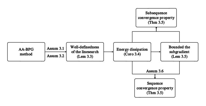
Figure 1: The flow chart of the convergence proof of Algorithm 1.

Under the 2, we have the following useful lemma as stated in [2].

Lemma 3.4 ([2]).

If $f$ is $R_{f}$-relative smooth with respect to $h$, then

(27) $$f(x)-f(y)-\langle\nabla f(y),x-y\rangle\leq R_{f}D_{h}(x,y),\quad\forall x,y\in\operatorname{\mathrm{int}\mathrm{dom}}h.$$

Based on the above Lemma, the descent property of the iteration generated by Bregman proximal operator Eq. 22 is established as follows.

Lemma 3.5.

Let $\alpha>0$ and suppose the 2 holds. If

(28) $$z=\operatorname*{\mathrm{argmin}}_{x}\left\{g(x)+\langle x-y,\nabla f(y)\rangle+\dfrac{1}{\alpha}D_{h}(x,y)\right\},$$

then there exists some $\sigma>0$ such that

(29) $$E(y)-E(z)\geq\left(\dfrac{1}{\alpha}-R_{f}\right)\frac{\sigma}{2}\|z-y\|^{2}.$$

Proof 3.6.

Since $h$ is strongly convex, there exists some constant $\sigma>0$ such that $h(x)-\sigma\|x\|^{2}/2$ is convex. Then, $\nabla^{2}h(x)-\sigma I\succeq 0$ and we have

(30) $$D_{h}(z,x)=h(z)-h(y)-\langle\nabla h(y),z-y\rangle\geq\frac{\sigma}{2}\|z-y\|^{2}.$$

From the optimal condition of Eq. 28, we have

$$E(y) =f(y)+g(y)=\left[f(y)+\langle\nabla f(y),x-y\rangle+\dfrac{1}{\alpha}D_{h}(x,y)+g(x)\right]_{x=y}$$

$$\geq f(y)+\langle\nabla f(y),z-y\rangle+\dfrac{1}{\alpha}D_{h}(z,y)+g(z)$$

$$\geq f(z)-R_{f}D_{h}(z,y)+\dfrac{1}{\alpha}D_{h}(z,y)+g(z)$$

$$=E(z)+\left(\dfrac{1}{\alpha}-R_{f}\right)D_{h}(z,y)\geq E(z)+\left(\dfrac{1}{\alpha}-R_{f}\right)\dfrac{\sigma}{2}\|z-y\|^{2},$$

where the second inequality is from Eq. 27 and the last inequality follows from Eq. 30.

Remark 3.7.

Lemma 3.5 shows that the non-restart condition Eq. 23 and the linear search condition Eq. 25 are satisfied when

(31) $$0<\alpha<\bar{\alpha}:=\min\left(\frac{1}{2c/\sigma+R_{f}},\frac{1}{2\eta/\sigma+R_{f}}\right)\mbox{ and }0<\alpha_{\min}\leq\bar{\alpha}$$

Therefore, the line search in Algorithm 2 stops in finite iterations, and thus the Algorithm 1 is well defined.

In the following analysis, we always assume that the parameter $\alpha_{\min}$ satisfies Eq. 31 for simplicity. Therefore, we can obtain the sufficient decrease property of the sequence generated by Algorithm 1.

Corollary 3.8.

Suppose the 3.1 and 2 hold. Let $\{x^{k}\}$ be the sequence generated by the Algorithm 1. Then, $\{x^{k}\}\subset\mathcal{M}(x^{0})$ and

(32) $$E(x^{k})-E(x^{k+1})\geq c_{0}\|x^{k}-x^{k+1}\|^{2},$$

where $c_{0}=\min(c,\eta)$.

The proof of Corollary 3.8 is a straightforward result as AA-BPG algorithm is well defined and the condition Eq. 23 or Eq. 25 holds at each iteration. Let $\mathcal{B}(x^{0})$ be the closed ball that contains $\mathcal{M}(x^{0})$. Since $h,F\in C^{2}$, there exist $\rho_{h},\rho_{f}>0$ such that

(33) $$\rho_{h}=\sup_{x\in\mathcal{B}(x^{0})}\|\nabla^{2}h(x)\|,\quad\rho_{f}=\sup_{x\in\mathcal{B}(x^{0})}\|\nabla^{2}f(x)\|.$$

Thus, we can show the subgradient of each step generated by Algorithm 1 is bounded by the movement of $x^{k}$.

Lemma 3.9 (Bounded the subgradient).

Suppose 3.1 and 2 holds. Let $\{x^{k}\}$ be the sequence generated by Algorithm 1. Then, there exists $c_{1}=\rho_{f}+\rho_{h}/\alpha_{\min}>0$ such that

(34) $$\mathrm{dist}(\mathbf{0},\partial E(x^{k+1}))\leq c_{1}(\|x^{k+1}-x^{k}\|+\bar{w}\|x^{k}-x^{k-1}\|),$$

where $\mathrm{dist}(\mathbf{0},\partial E(x^{k+1}))=\inf\{\|y\|:y\in\partial E(x^{k+1})\}$ and $\rho_{h}$, $\rho_{f}$ are defined as Eq. 33 and $\bar{w},\alpha_{\min}$ are constants defined in Algorithm 1 and Algorithm 2, respectively.

Proof 3.10.

By the first order optimality condition of Eq. 21, we get

$$\mathbf{0}\in\nabla f(y^{k})+\dfrac{1}{\alpha_{k}}\left(\nabla h(x^{k+1})-\nabla h(y^{k})\right)+\partial g(x^{k+1})$$

$$\iff -\nabla f(y^{k})-\dfrac{1}{\alpha_{k}}\left(\nabla h(x^{k+1})-\nabla h(y^{k})\right)\in\partial g(x^{k+1})$$

Since $f\in C^{2}$, we know [39, Theorem 5.38]

(35) $$\partial E(x)=\nabla f(x)+\partial g(x).$$

From Lemma 3.5, we have $x^{k},x^{k-1}\in\mathcal{M}(x^{0})$, then $y^{k}=(1+w_{k})x^{k}-w_{k}x^{k-1}\in\mathcal{B}(x^{0})$. Together with (35), we have

$$\mathrm{dist}(\mathbf{0},\partial E(x^{k+1})) =\inf_{y\in\partial g(x^{k+1})}\|\nabla f(x^{k+1})+y\|$$

$$\leq\|\nabla f(x^{k+1})-\nabla f(y^{k})-\dfrac{1}{\alpha_{k}}\left(\nabla h(x^{k+1})-\nabla h(y^{k})\right)\|$$

$$\leq\|\nabla f(x^{k+1})-\nabla f(y^{k})\|+\dfrac{1}{\alpha_{k}}\|\nabla h(x^{k+1})-\nabla h(y^{k})\|$$

$$\leq(\rho_{f}+\dfrac{\rho_{h}}{\alpha_{k}})\|x^{k+1}-y^{k}\|$$

$$\leq c_{1}(\|x^{k+1}-x^{k}\|+\bar{w}\|x^{k}-x^{k-1}\|),$$

where the last inequality is from $y^{k}=x^{k}+w_{k}(x^{k}-x^{k-1})$ and $w^{k}\in[0,\bar{w}]$.

Now, we are ready to establish the sub-convergence property of Algorithm 1.

Theorem 3.

Suppose 3.1 and 2 hold. Let $\{x^{k}\}$ be the sequence generated by Algorithm 1. Then, for any limit point $x^{*}$ of $\{x^{k}\}$, we have $\mathbf{0}\in\partial E(x^{*})$.

Proof 3.11.

From Corollary 3.8, we know $\{x^{k}\}\subset\mathcal{M}(x^{0})\subset\mathcal{B}(x^{0})$ and thus bounded. Then, the set of limit points of $\{x^{k}\}$ is nonempty. For any limit point $x^{*}$, there exist a subsequence $\{x^{k_{j}}\}$ such that $x^{k_{j}}\to x^{*}$ as $j\to\infty$. We know $\{E(x^{k})\}$ is a decreasing sequence. Together with the fact that $E$ is bounded below, there exists some $\bar{E}$ such that $E(x^{k})\to\bar{E}$ as $k\to\infty$. Moverover, it has

(36) $$E(x^{0})-\bar{E}=\lim_{K\to\infty}\sum_{j=0}^{K}\left(E(x^{j})-E(x^{j+1})\right)\geq c_{0}\lim_{K\to\infty}\sum_{j=0}^{K}\|x^{j}-x^{j+1}\|^{2},$$

and implies $\|x^{k}-x^{k-1}\|\to 0$ as $k\to\infty$. As a result,

$$\lim\limits_{k\to\infty}\|x^{k}-y^{k-1}\|\leq\lim\limits_{k\to\infty}(\|x^{k}-x^{k-1}\|+\bar{\omega}\|x^{k-1}-x^{k-2}\|)=0.$$

Together with Eq. 34, it implies that there exists $u^{k_{j}}\in\partial g(x^{k_{j}})$ such that

(37) $$\lim_{j\to\infty}\|\nabla f(x^{k_{j}})+u^{k_{j}}\|=0\Rightarrow\lim_{j\to\infty}u^{k_{j}}=-\nabla f(x^{*}),$$

as $\nabla f$ is continuous and $x^{k_{j}}\to x^{*}$ when $j\to\infty$.

In the next, we prove $\lim\limits_{j\to\infty}g(x^{k_{j}})=g(x^{*})$. It is easy to know that $\lim\limits_{j\to\infty}x^{k_{j}-p}=x^{*}$ for finite $p\geq 0$ since $\lim\limits_{k\to\infty}\|x^{k}-x^{k-1}\|=0$. Thus, we have $y^{k_{j}-1}=x^{k_{j}-1}+w_{k_{j}-1}(x^{k_{j}-1}-x^{k_{j}-2})\to x^{*}$ as $j\to\infty$. From Eq. 21, we know

(38) $$\begin{split}&g(x^{k_{j}})+\langle x^{k_{j}}-y^{k_{j}-1},\nabla f(y^{k_{j}-1})\rangle+\dfrac{1}{\alpha_{k}}D(x^{k_{j}},y^{k_{j}-1})\\ \leq~{}&g(x)+\langle x-y^{k_{j}-1},\nabla f(y^{k_{j}-1})\rangle+\dfrac{1}{\alpha_{k}}D(x,y^{k_{j}-1}),\quad\forall x.\end{split}$$

Let $x=x^{*}$ and $j\to\infty$, we get $\limsup\limits_{j\to\infty}g(x^{k_{j}})\leq g(x^{*})$. By the fact that $g(x)$ is lower semi-continuous, it has $\lim\limits_{j\to\infty}g(x^{k_{j}})=g(x^{*})$.

Thus, by the convexity of $g$, we have

(39) $$g(x)\geq g(x^{k_{j}})+\langle u^{k_{j}},x-x^{k_{j}}\rangle,\forall x\in\mathrm{dom}g.$$

Let $j\to\infty$ in (39) and using the facts $x^{k_{j}}\to x^{*}$, $g(x^{k_{j}})\to g(x^{*})$ as $j\to\infty$ and (37), we have $-\nabla f(x^{*})\in\partial g(x^{*})$ and thus $0\in\partial E(x^{*})$.

Furthermore, the sub-sequence convergence can be strengthen by imposing the next assumption on $E$ which is known as the Kurdyka-Lojasiewicz (KL) property [4].

Assumption 4.

$E(x)$ is the $KL$ function, i.e. for all $\bar{x}\in\mathrm{dom}\partial E:=\{x:\partial E(x)\neq\emptyset\}$, there exist $\eta>0$, a neighborhood $U$ of $\bar{x}$ and $\psi\in\Psi_{\eta}:=\{\psi\in C[0,\eta)\cap C^{1}(0,\eta),\text{ where }\psi\text{ is concave},\psi(0)=0,\psi^{{}^{\prime}}>0\text{ on }(0,\eta)\}$ such that for all $x\in U\cap\{x:E(\bar{x})<E(x)<E(\bar{x})+\eta\}$, the following inequality holds,

(40) $$\psi^{{}^{\prime}}(E(x)-E(\bar{x}))\,\mathrm{dist}(\mathbf{0},\partial E(x))\geq 1.$$

Theorem 5.

Suppose 3.1, 2 and 4 hold. Let $\{x^{k}\}$ be the sequence generated by Algorithm 1. Then, there exists a point $x^{*}\in\mathcal{B}(x^{0})$ such that

(41) $$\lim\limits_{k\rightarrow+\infty}x^{k}=x^{*},\quad\mathbf{0}\in\partial E(x^{*}).$$

Proof 3.12.

The proof is in Appendix A.

It is known from [4] that many functions satisfy 4 including the energy function in PFC models. In the following context, we apply the AA-BPG method for solving the PFC models Eq. 15 by introducing two Bregman distances.

4 AA-BPG method for solving PFC models

The problem Eq. 15 can be reduced to Eq. 18 by setting

(42) $$f(\hat{\Phi})=F(\hat{\Phi}),\quad g(\hat{\Phi})=G(\hat{\Phi})+\delta_{\mathcal{S}}(\hat{\Phi})$$

where $\mathcal{S}=\{\hat{\Phi}:e_{1}^{\top}\hat{\Phi}=0\}$ and $\delta_{\mathcal{S}}(\hat{\Phi})=0$ if $\hat{\Phi}\in\mathcal{S}$ and $+\infty$ otherwise. The main difficulty of applying Algorithm 1 is solving the subproblem Eq. 22 efficiently. In this section, two different strongly convex functions $h$ are chosen as

(43) $$h(x)=\frac{1}{2}\|x\|^{2}~{}\mbox{ (P2) }\quad\mbox{ and }\quad h(x)=\frac{a}{4}\|x\|^{4}+\frac{b}{2}\|x\|^{2}+1~{}\mbox{ (P4), }$$

where $a,b>0$ and (P2) and (P4) represent the highest order of the $\ell^{2}$ norm.

Case (P2). The Bregman distance of $D_{h}$ is reduced to the Euclidean distance, i.e.

(44) $$D_{h}(x,y)=\dfrac{1}{2}\|x-y\|^{2}.$$

The subproblem Eq. 22 is reduced to

(45) $$\min_{\hat{\Phi}}~{}G(\hat{\Phi})+\langle\nabla F(\hat{\Psi}^{k}),\hat{\Phi}-\hat{\Psi}^{k}\rangle+\frac{1}{2\alpha_{k}}\|\hat{\Phi}-\hat{\Psi}^{k}\|^{2},\mbox{ s.t. }e_{1}^{\top}\hat{\Phi}=0,$$

where $\hat{\Psi}^{k}=\hat{\Phi}^{k}+w_{k}(\hat{\Phi}^{k}-\hat{\Phi}^{k-1})$. Although the Eq. 45 is a constrained minimization problem, it has a closed form solution based on our discretization which leads to a fast computation.

Lemma 4.1.

Given $\alpha_{k}>0$, if $e_{1}^{\top}\hat{\Psi}^{k}=0$, the minimizer of Eq. 45, denoted by $\hat{\Phi}^{k+1}$, is given by

(46) $$\hat{\Phi}^{k+1}=\left(I+\alpha_{k}D\right)^{-1}\left(\hat{\Psi}^{k}-\alpha_{k}\mathcal{P}_{1}\nabla F(\hat{\Psi}^{k})\right),$$

where $D$ is defined in Eq. 16 and $\mathcal{P}_{1}=I-e_{1}e_{1}^{\top}$ is the projection into the set $\mathcal{S}$.

Proof 4.2.

The KKT conditions for this subproblem Eq. 22 can be written as

(47) $$\nabla G(\hat{\Phi}^{k+1})+\nabla F(\hat{\Psi}^{k})+\dfrac{1}{\alpha_{k}}\left(\hat{\Phi}^{k+1}-\hat{\Psi}^{k}\right)-\xi_{k}e_{1}=0,$$

(48) $$e_{1}^{\top}\hat{\Phi}^{k+1}=0,$$

where $\xi_{k}$ is the Lagrange multiplier. Taking the inner product with $e_{1}$ in Eq. 47, we obtain

$$\xi_{k}=e_{1}^{\top}\left(\nabla G(\hat{\Phi}^{k+1})+\nabla F(\hat{\Phi}^{k})-\dfrac{1}{\alpha_{k}}\hat{\Psi}^{k}\right).$$

Using Eq. 48 and Eq. 16, we know

$$e_{1}^{\top}\nabla G(\hat{\Phi}^{k+1})=e_{1}^{\top}(D\hat{\Phi}^{k+1})=0.$$

Together with $e_{1}^{\top}\hat{\Psi}^{k}=0$, we have $\xi_{k}=e_{1}^{\top}\nabla F(\hat{\Psi}^{k})$. Substituting it into Eq. 47, it follows that

$$\hat{\Phi}^{k+1} =\left(\alpha_{k}D+I\right)^{-1}\left(\hat{\Psi}^{k}-\alpha_{k}\mathcal{P}_{1}\nabla F(\hat{\Psi}^{k})\right).$$

It is noted that from the proof of Lemma 4.1, the feasibility assumption $e_{1}^{\top}\hat{\Psi}^{k}=0$ holds as long as $e_{1}^{\top}\hat{\Phi}^{0}=0$ which can be set in the initialization. The detailed algorithm is given in Algorithm 3 with $K=2$.

Case (P4). In this case, the subproblem Eq. 22 is reduced to

(49) $$\min_{\hat{\Phi}}G(\hat{\Phi})+\langle\nabla F(\hat{\Psi}^{k}),\hat{\Phi}-\hat{\Psi}^{k}\rangle+D_{h}(\hat{\Phi},\hat{\Psi}^{k}),\mbox{ s.t. }e_{1}^{\top}\hat{\Phi}=0.$$

where $\hat{\Psi}^{k}=\hat{\Phi}^{k}+w_{k}(\hat{\Phi}^{k}-\hat{\Phi}^{k-1})$. The next lemma shows the optimal condition of minimizing Eq. 49.

Lemma 4.3.

Given $\alpha^{k}>0$. If $e_{1}^{\top}\hat{\Psi}^{k}=0$, the minimizer of Eq. 49, denoted by $\hat{\Phi}^{k+1}$, is given by

(50) $$\hat{\Phi}^{k+1}=[\alpha_{k}D+(ap^{*}+b)I]^{-1}(\nabla h(\hat{\Psi}^{k})-\alpha_{k}\mathcal{P}_{1}\nabla F(\hat{\Psi}^{k})),$$

where $D$ is given in Eq. 16 and $p^{*}$ is a fixed point of $p=\|\hat{\Phi}^{k+1}\|^{2}:=r(p)$.

Proof 4.4.

The KKT conditions of Eq. 49 imply that there exists a Lagrange multiplier $\xi_{k}$ such that $(\hat{\Phi}^{k+1},\xi_{k})$ satisfies

(51) $$\alpha_{k}\nabla G(\hat{\Phi}^{k+1})+\alpha_{k}\nabla F(\hat{\Psi}^{k})+\nabla h(\hat{\Phi}^{k+1})-\nabla h(\hat{\Psi}^{k})-\xi_{k}e_{1}=0,$$

(52) $$e_{1}^{\top}\hat{\Phi}^{k+1}=0.$$

Since $e_{1}^{\top}\hat{\Phi}^{k}=0$ and $\nabla h(x)=(a\|x\|^{2}+b)x$, Eq. 52 and Eq. 16 imply

$$e_{1}^{\top}\nabla G(\hat{\Phi}^{k+1})=e_{1}^{\top}(D\hat{\Phi}^{k+1})=0,\quad e_{1}^{\top}\nabla h(\hat{\Psi}^{k})=(a\|\hat{\Psi}^{k}\|^{2}+b)e_{1}^{\top}\hat{\Psi}^{k}=0,$$

where $D$ is defined in Eq. 16. Substituting the above equalities into Eq. 51 implies $\xi_{k}=\alpha_{k}e_{1}^{\top}\nabla F(\hat{\Psi}^{k})$. Denote

$$p:=\|\hat{\Phi}^{k+1}\|^{2}\geq 0,\quad\beta:=\nabla h(\hat{\Psi}^{k})-\alpha_{k}\nabla F(\hat{\Psi}^{k})+\xi e_{1}=\nabla h(\hat{\Psi}^{k})-\alpha_{k}\mathcal{P}_{1}\nabla F(\hat{\Psi}^{k}).$$

From Eq. 51, we obtain a fixed point problem with respect to $p$

(53) $$p=\|\hat{\Phi}^{k+1}\|^{2}=\|[D+(ap+b)I]^{-1}\beta\|^{2}:=r(p).$$

Let $R(p)=r(p)-p$. Then $R(0)=\|(D+bI)^{-1}\beta\|^{2}\geq 0$, $R(p)\to-\infty$ as $p\to\infty$ and

$$R^{\prime}(p)=-2a\sum_{i=1}^{n}\dfrac{\beta_{i}^{2}}{(D_{ii}+ap+b)^{3}}-1<0,\quad\forall p\geq 0,$$

there is an unique zero $p^{*}\geq 0$ of $R(p)$, i.e. $p^{*}=r(p^{*})$. Thus,

$$\hat{\Phi}^{k+1}=[\alpha_{k}D+(ap^{*}+b)I]^{-1}(\nabla h(\hat{\Psi}^{k})-\alpha_{k}\mathcal{P}_{1}\nabla F(\hat{\Psi}^{k})).$$

It is noted that the fixed point equation Eq. 53 is a nonlinear scalar equation which can efficiently solved by many existing solvers. The detailed algorithm is given in Algorithm 3 with $K=4$.

Algorithm 3 AA-BPG-K method for PFC model

0:  $\hat{\Phi}^{1}=\hat{\Phi}^{0}$, $\alpha_{0}>0$, $w_{0}\in[0,1]$, $\rho\in(0,1)$, $\eta,c,\bar{w}>0$ and $k=1$.

1:  while  stop criterion is not satisfied do

2:     Update $\hat{\Psi}^{k}=\hat{\Phi}^{k}-w_{k}(\hat{\Phi}^{k}-\hat{\Phi}^{k-1})$

3:     Estimate $\alpha_{k}$ by Algorithm 2

4:     if $K=2$ then

5:        Calculate $z^{k}=\left(\alpha_{k}D+I\right)^{-1}\left(\hat{\Psi}^{k}-\alpha_{k}\mathcal{P}_{1}\nabla F(\hat{\Psi}^{k})\right)$

6:     else if $K=4$ then

7:        Calculate the fixed point of Eq. 53.

8:        Calculate $z^{k}=[\alpha_{k}D+(ap^{*}+b)I]^{-1}(\nabla h(\hat{\Psi}^{k})-\alpha_{k}\mathcal{P}_{1}\nabla F(\hat{\Psi}^{k}))$

9:     end if

10:     if $E(\hat{\Phi}^{k})-E(z^{k})\geq c\|\hat{\Phi}^{k}-z^{k}\|^{2}$  then

11:        $\Phi^{k+1}=z^{k}$ and update $w_{k+1}\in[0,\bar{w}]$.

12:     else

13:        $\Phi^{k+1}=\Phi^{k}$ and reset $w_{k+1}=0$.

14:     end if

15:     $k=k+1$.

16:  end while

4.1 Convergence analysis for Algorithm 3

The convergence analysis can be directly applied for Algorithm 3 if the assumptions required in 3 hold. We first show that the energy function $E$ in PFC model satisfies 3.1 and 4. Then, 2 is analyzed for Case (P2) and Case (P4) independently.

Lemma 4.5.

Let $E_{0}=F(\hat{\Phi})+G(\hat{\Phi})$ and $E(\hat{\Phi})=E_{0}(\hat{\Phi})+\delta_{\mathcal{S}}(\hat{\Phi})$ be the energy functional which is defined in Eq. 42. Then, it satisfies

1. $E$ is bounded below and the sub-level set $\mathcal{M}(\hat{\Phi}^{0})$ is compact for any $\hat{\Phi}^{0}\in\mathcal{S}$.

2. $E$ is a KL function, and thus satisfies 4.

Proof 4.6.

From the continuity and the coercive property of $F$, i.e. $F(\hat{\Phi})\to+\infty$ as $\hat{\Phi}\to\infty$, the sub-level set $\mathcal{S}_{0}:=\{\hat{\Phi}:E_{0}(\hat{\Phi})\leq E_{0}(\hat{\Phi}^{0})\}$ is compact for any $\hat{\Phi}^{0}$. Together with $\mathcal{S}$ is closed, it follows that $\mathcal{M}(\hat{\Phi}^{0})=\mathcal{S}\cap\mathcal{S}_{0}$ is compact for any $\hat{\Phi}^{0}$.

Moreover, according to Example 2 in [4], it is easy to know that $E(\hat{\Phi})$ is semi-algebraic function, then it is KL function by Theorem 2 in  [4].

Lemma 4.7.

Let $F(\hat{\Phi})$ be defined in Eq. 15. Then, we have

1. If $h$ is chosen as (P2) in Eq. 43, then $F$ is relative smooth with respect to $h$ in $\mathcal{M}$ for any compact set $\mathcal{M}$.

2. If $h$ is chosen as (P4) in Eq. 43, then $F$ is relative smooth with respect to $h$.

Proof 4.8.

Denote $\hat{\Phi}^{\otimes k}:=\hat{\Phi}\otimes\hat{\Phi}\otimes\cdots\otimes\hat{\Phi}$ where $\otimes$ is the tensor product. Then, $F(\hat{\Phi})$ is the $4th$-degree polynomial, i.e. $F(\hat{\Phi})=\sum_{k=2}^{4}\langle\mathcal{A}_{k},\hat{\Phi}^{\otimes k}\rangle$ where the $kth$-degree monomials are arranged as a $kth$-order tensor $\mathcal{A}_{k}$. For any compact set $\mathcal{M}$, $\nabla^{2}F$ is bounded and thus $F$ is relative smooth with respect to any polynomial function in $\mathcal{M}$ which includes case (P2). When $h$ is chosen as (P4), according to Lemma 2.1 in [24], there exists $R_{F}>0$ such that $F(\hat{\Phi})$ is $R_{F}$-relative smooth with respect to $h(x)$.

Combining Lemma 4.5, Lemma 4.7 with 5, we can directly establish the convergence of Algorithm 3 .

Theorem 1.

Let $E(\hat{\Phi})=F(\hat{\Phi})+G(\hat{\Phi})+\delta_{\mathcal{S}}(\hat{\Phi})$ be the energy function which is defined in Eq. 42. The following results hold.

1. Let $\{\hat{\Phi}^{k}\}$ be the sequence generated by Algorithm 3 with $K=2$. If $\{\hat{\Phi}^{k}\}$ is bounded, then $\{\hat{\Phi}^{k}\}$ converges to some $\hat{\Phi}^{*}$ and $0\in\partial E(\hat{\Phi}^{*})$.

2. Let $\{\hat{\Phi}^{k}\}$ be the sequence generated by Algorithm 3 with $K=4$. Then, $\{\hat{\Phi}^{k}\}$ converges to some $\hat{\Phi}^{*}$ and $0\in\partial E(\hat{\Phi}^{*})$.

It is noted that when $h$ is chosen as (P2), we cannot bounded the growth of $F$ as $F$ is a fourth order polynomial. Thus, the boundedness assumption of $\{\hat{\Phi}^{k}\}$ is imposed which is similar to the requirement in the semi-implicit scheme [33].

5 Newton-PCG method

Despite the fast initial convergence speed of the gradient based methods, the tail convergence speed becomes slow. Therefore it can be further locally accelerated by the feature of Hessian based methods. In this section, we design a practical Newton method to solve the PFC models Eq. 15 and provide a hybrid accelerated framework.

5.1 Our method

Define $Z:=[0,I_{N-1}]^{\top}$, any vector $\hat{\Phi}$ that satisfies the constraint $e_{1}^{\top}\hat{\Phi}=0$ has the form of $\hat{\Phi}=ZU$ with $U\in\mathbb{C}^{N-1}$. Since $Z^{\top}Z=I_{N-1}$, we can also obtain $U$ from $\hat{\Phi}$ by $U=Z^{\top}\hat{\Phi}$. Therefore, the problem Eq. 15 is equivalent to

(54) $$\min_{U\in\mathbb{C}^{N-1}}E(ZU)=G(ZU)+F(ZU).$$

Let $\tilde{E}(U):=E(ZU),\,\tilde{G}(U):=E(ZU),\,\tilde{F}(U):=F(ZU)$, we have the following facts

(55) $$\tilde{g}:=\nabla\tilde{E}(U)=Z^{\top}\nabla E(ZU)=Z^{\top}g,$$

$$\tilde{\mathcal{J}}:=\nabla^{2}\tilde{E}(U)=Z^{\top}\nabla^{2}E(ZU)Z=Z^{\top}\mathcal{J}Z,$$

where $g=\nabla E(ZU)$ and $\mathcal{J}=\nabla^{2}E(ZU)$. Therefore, finding the steady states of PFC models is equivalent to solving the nonlinear equations

(56) $$\nabla\tilde{E}(U)=\mathbf{0}.$$

Due to the non-convexity of $\tilde{E}(U)$, the Hessian matrix $\tilde{\mathcal{J}}$ may not be positive definite and thus a regularized Newton method is applied.

Computing the Newton direction. Denote $\tilde{\mathcal{J}}_{k}:=\nabla^{2}\tilde{E}(U^{k})$ and $\tilde{g}_{k}:=\nabla\tilde{E}(U^{k})$, we find the approximated Newton direction $d_{k}$ by solving

(57) $$(\tilde{\mathcal{J}}_{k}+\mu_{k}I)d_{k}=-\tilde{g}_{k},$$

where regularized parameter $\mu_{k}$ is chosen as

(58) $$-c_{1}\min\{0,\lambda_{\min}(\tilde{\mathcal{J}}_{k})\}+c_{2}\|\tilde{g}_{k}\|\leq\mu_{k}\leq\bar{\mu}<+\infty~{}(c_{1}\geq 1,c_{2}>0).$$

Thus, Eq. 57 is symmetric, positive definite linear system. To accelerate the convergence, an preconditioned conjugate gradient (PCG) method is adopted. More specifically, in $k$-th step, we terminate the PCG iterates whenever $\|(\tilde{\mathcal{J}}_{k}+\mu_{k}I)d_{k}+\tilde{g}_{k}\|\leq\eta_{k}$ in which $\eta_{k}$ is set as

(59) $$\eta_{k}=\tau\min\{1,\|\tilde{g}_{k}\|\},\quad 0<\tau<1,$$

and the preconditioner $M_{k}$ is adaptively obtained by setting

(60) $$M_{k}=Z(H_{k}+\mu_{k}I)^{-1}Z^{\top}\quad\mbox{with}\quad H_{k}=D+\delta_{k}I$$

where $D$ is from Eq. 16 and some $\delta_{k}>0$. Let $A=\tilde{\mathcal{J}}_{k}+\mu_{k}I$, $b=-\tilde{g}_{k}$ and $M=M_{k}$, the PCG method is given in Algorithm 4, where $\|x\|_{A}:=\langle x,Ax\rangle$.

Algorithm 4 PCG($\eta$) for solving $Ax=b$.

0:  $A,b,\eta,k_{max}$, preconditioner $M$.

1:  Set $x^{0}=0,r_{0}=Ax^{0}-b=-b,p_{0}=-M^{-1}r_{0},i=0$.

2:  while $\|r_{i}\|>\eta$ or $i<k_{max}$ do

3:     $\alpha_{i+1}=\dfrac{\|r_{i}\|_{M^{-1}}^{2}}{\|p_{i}\|_{A}^{2}}$

4:     $x^{i+1}=x^{i}+\alpha_{i+1}p_{i}$

5:     $r_{i+1}=r_{i}+\alpha_{i+1}Ap_{i}$

6:     $\beta_{i+1}=\dfrac{\|r_{i+1}\|_{M^{-1}}^{2}}{\|r_{i}\|_{M^{-1}}^{2}}$

7:     $p_{i+1}=-M^{-1}r_{i+1}+\beta_{i+1}p_{i}$

8:     $i=i+1$

9:  end while

Computing the step size $t_{k}$. Once the Newton direction $d_{k}$ is obtained, the line search technique is applied for finding an appropriate step size $t_{k}$ that satisfies the following inequality:

(61) $$\tilde{E}(U^{k}+t_{k}d_{k})\leq\tilde{E}(U^{k})+\nu t_{k}\langle\tilde{g}_{k},d_{k}\rangle,~{}0<\nu<1.$$

The existence of $t_{k}>0$ that satisfies Eq. 61 is given in Lemma 5.5. Then, $U^{k+1}$ is updated by $U^{k+1}=U^{k}+t_{k}d_{k}$. Our proposed algorithm is summarized in Algorithm 5.

Algorithm 5 Newton-PCG method

0:  $U^{0},\varepsilon,\bar{\mu},c_{1}\geq 1,c_{2}>0,0<\nu,\rho,\tau<1;$

1:  $k=0,\tilde{g}_{0}=\nabla\tilde{E}(U^{0})$;

2:  while stop criterion is not satisfied do

3:     Choose $-c_{1}\min\{0,\lambda_{\min}(\tilde{\mathcal{J}}_{k})\}+c_{2}\|\tilde{g}_{k}\|\leq\mu_{k}\leq\bar{\mu}$;

4:     Update $\eta_{k}=\tau\min(1,\|\tilde{g}_{k}\|)$.

5:     Find direction $d_{k}$ by solving Eq. 57 via PCG($\eta_{k}$) using Algorithm 4;

6:     for $n=0,1,2,\cdots$ do

7:        $t_{k}=\rho^{n};$

8:        if $\tilde{E}(U^{k}+t_{k}d_{k})\leq\tilde{E}(U^{k})+\nu t_{k}\langle\tilde{g}_{k},d_{k}\rangle$ then

9:           Break;

10:        end if

11:     end for

12:     $U^{k+1}=U^{k}+t_{k}d_{k}$;

13:     $k=k+1;$

14:  end while

5.2 Convergence analysis for Algorithm 5

We first establish several properties related to the direction $d_{k}$ computed by the PCG method.

Lemma 5.1.

Consider a linear system $Ax=b$ where $A$ is symmetric and positive definite. Let $\{x^{i}\}$ be the sequence generated by Algorithm 4, it satisfies

(62) $$\dfrac{1}{\lambda_{\max}(A)}\leq\dfrac{\langle x^{i},b\rangle}{\|b\|^{2}}\leq\dfrac{1}{\lambda_{\min}(A)},\quad\forall i=1,2,\cdots.$$

Proof 5.2.

The proof is in Appendix B.

Then, we know the $d_{k}$ is a descent direction from the next lemma.

Lemma 5.3 (Descent direction).

Let $d_{k}$ be generated by PCG($\eta_{k}$) method (Algorithm 4). If $\|\tilde{g}_{k}\|>0$, then we have

(63) $$-\langle d_{k},\tilde{g}_{k}\rangle\geq l_{k}:=\dfrac{\|\tilde{g}_{k}\|^{2}}{\lambda_{\max}(\tilde{\mathcal{J}}_{k}+\mu_{k}I)}\quad\mbox{and}\quad\|d_{k}\|\leq\bar{d}:=\dfrac{\tau+1}{c_{2}},$$

where $\tau$, $K$, and $c_{1},c_{2}$ are defined in Eq. 59, Eq. 68 and Eq. 58, respectively.

Proof 5.4.

The first inequality is a direct consequence of Lemma 5.1. Moreover, let $r_{k}=(\tilde{\mathcal{J}}_{k}+\mu_{k}I)d_{k}+\tilde{g}_{k}$. By Algorithm 4 and Eq. 59, we have $\|r_{k}\|\leq\eta_{k}\leq\tau\|\tilde{g}_{k}\|$. Then,

$$\|d_{k}\| =\|(\tilde{\mathcal{J}}_{k}+\mu_{k}I)^{-1}(r_{k}-\tilde{g}_{k})\|\leq\dfrac{\|r_{k}-\tilde{g}_{k}\|}{\lambda_{\min}(\tilde{\mathcal{J}}_{k}+\mu_{k}I)}\leq\dfrac{\|r_{k}\|+\|g_{k}\|}{c_{2}\|g_{k}\|}\leq\dfrac{\tau+1}{c_{2}},$$

where the second inequality is from Eq. 58.

Lemma 5.5 (Lower bound of $t_{k}$).

Let $d_{k}$ be generated by PCG($\eta_{k}$) method (Algorithm 4). If $\|\tilde{g}_{k}\|\geq\varepsilon>0$, then for any $\nu\in(0,1)$, there exists $M_{k}>0$ and

(64) $$t_{\max}^{k}:=\min\left\{\frac{2(1-\nu)l_{k}}{M_{k}\bar{d}^{2}},1\right\}.$$

such that the inequality Eq. 61 holds for $t_{k}\in(0,t_{\max}^{k}]$ where $l_{k}$ is defined in Eq. 63.

Proof 5.6.

By the Taylor expansion, we have

(65) $$\tilde{E}(U^{k}+td_{k})=\tilde{E}(U^{k})+t\langle\tilde{g}_{k},d_{k}\rangle+\dfrac{t^{2}}{2}\langle d_{k},\nabla^{2}\tilde{E}(\xi^{t})d_{k}\rangle,$$

where $\xi^{t}\in\mathcal{V}_{k}=\{V|V=U^{k}+td_{k},t\in[0,1]\}$. As $\tilde{E}\in C^{2}$, there exists $M_{k}>0$ such that $M_{k}=\sup\{\|\nabla^{2}\tilde{E}(V)\|\}|V\in\mathcal{V}_{k}\}$. Then, Eq. 65 and Eq. 63 imply

(66) $$\tilde{E}(U^{k}+td_{k}) \leq\tilde{E}(U^{k})+\nu t\langle\tilde{g}_{k},d_{k}\rangle-(1-\nu)l_{k}t+\dfrac{M_{k}\bar{d}^{2}}{2}t^{2}.$$

Define $Q(t)=(1-\nu)l_{k}t-\dfrac{M_{k}\bar{d}^{2}}{2}t^{2}$, we know $Q(t)\geq 0$ for all $t\in[0,\dfrac{2(1-\nu)l_{k}}{M_{k}\bar{d}^{2}}]$ which implies Eq. 61 holds for all $t\in(0,t_{\max}^{k}]$.

Theorem 5.7.

Let $\tilde{E}$ be defined in Eq. 54 and $\{U^{k}\}$ be the infinite sequence generated by Algorithm 5. Then $\{U^{k}\}$ is bounded and has the following property:

(67) $$\lim\limits_{k\rightarrow+\infty}\|\tilde{g}_{k}\|=0.$$

Proof 5.8.

Due to the continuity of $\tilde{F}$, $\tilde{G}$ in Eq. 54 and the coercive property of $\tilde{F}$, the sublevel set $\mathcal{M}_{0}=\{U:\tilde{E}(U)\leq\tilde{E}(U^{0})\}$ is compact for any $U^{0}$. By the inequality Eq. 61, it is easy to know $\{\tilde{E}(U^{k})\}$ is a decreasing sequence, and thus $\{U^{k}\}\subset\mathcal{M}_{0}$ a nd there exists some $\bar{E}$ such that $\tilde{E}(U^{k})\to\bar{E}$ as $k\to\infty$. Moreover, from Eq. 63 and $t_{k}\in(0,1]$, we know there exist a compact set $\mathcal{B}_{0}$ such that $\{U^{k}+td^{k}|t\in(0,1]\}\subset\mathcal{B}_{0}$ and thus there exists $M>0$ such that

(68) $$\|\nabla^{2}\tilde{E}(U)\|\leq M,\quad\forall\,U\in\mathcal{B}_{0}.$$

From the proof of Lemma 5.5, we know $M_{k}\leq M$ for all $k$. Moreover, there exists some $\bar{\lambda}>0$ such that $\lambda_{\max}(\tilde{\mathcal{J}}_{k}+\mu_{k}I)\leq\bar{\lambda}$ for all $k$. We prove Eq. 67 by contradiction. Assume $\limsup\limits_{k\rightarrow+\infty}\|\tilde{g}_{k}\|=\varepsilon>0$ and define the index set

(69) $$\mathcal{I}=\cup_{k=1}^{\infty}\mathcal{I}_{k}:=\left\{j\in\mathbb{N}:j\leq k,\|\tilde{g}_{j}\|\geq\varepsilon/2\right\}.$$

Then, we know $|\mathcal{I}|=\infty$ where $|\mathcal{I}|$ denotes the number of the elements of $\mathcal{I}$. Moreover, for all $j\in\mathcal{I}$, we know

(70) $$l_{j}\geq\varepsilon/2\bar{\lambda}\quad\mbox{ and }\quad t_{\max}^{j}\geq\bar{t}=\min\left\{\dfrac{(1-\nu)\varepsilon}{M\bar{\lambda}\bar{d}^{2}},1\right\}.$$

Thus, $\bar{t}$ is a uniform lower bound for the step size $t$ at $U^{j}$ for $j\in\mathcal{I}$, i.e. $t_{j}\geq t,\forall j\in\mathcal{I}$, and we have

(71) $$\tilde{E}(U^{0})-\tilde{E}(U^{k+1}) =\sum_{j=0}^{k}(\tilde{E}(U^{j})-\tilde{E}(U^{j+1}))\geq\sum_{j\in\mathcal{I}_{k}}(\tilde{E}(U^{j})-\tilde{E}(U^{j+1}))$$

(72) $$\geq\sum_{j\in\mathcal{I}_{k}}-\nu t_{j}\langle\tilde{g}_{j},d_{j}\rangle\geq\dfrac{\nu\bar{t}\varepsilon}{2\bar{\lambda}}|\mathcal{I}_{k}|,$$

Let $k\to\infty$ in Eq. 71, we know $\tilde{E}(U^{0})-\bar{E}\geq+\infty$, which leads to a contradiction.

5.3 Hybrid acceleration framework

Many gradient based methods have a good convergent performance at the beginning, but often show slow tail convergence near the stationary states. In this case, the Newton-like method is a natural choice and has a better convergence speed when the iteration is near the stationary states. It is noted that the Hessian based method is sensitive to the initial point. A key step of mixing two methods is designing a proper criterion to determine when to launch the Hessian based method. It is difficult to develop a perfect strategy for all kinds of PFC models. In our experiments, we switch to the Newton-PCG algorithm when one of the following criteria is met

(73) $$|E(\hat{\Phi}^{k})-E(\hat{\Phi}^{k-1})|<\varepsilon_{1}\quad\mbox{or}\quad\|g_{k}-g_{k-1}\|<\varepsilon_{2},$$

where $\varepsilon_{1},\varepsilon_{2}>0$. Our proposed hybrid accelerated framework is summarized in Algorithm 6. The M method stands for a certain existing method, such as our AA-BPG method.

Algorithm 6 Hybrid acceleration framework (N-M method)

0:  $\Phi^{0},\varepsilon_{1},\varepsilon_{2}$ and $k=0$.

1:  while  stop criterion is not satisfied do

2:     if switching condition is satisfed then

3:        Perform Newton-PCG method (Algorithm 5);

4:     else

5:        Perform M method;

6:     end if

7:     $k=k+1$;

8:  end while

Remark 5.9.

The idea of hybrid method provides a general framework for local acceleration. Our Newton-PCG methods can not only combines with the AA-BPG methods, but also with many existing methods. It’s worth noting that directly using the Newton-PCG method may converge to a bad stationary point or lead to slow convergence since the initial point is not good.

6 Numerical results

In this section, we present several numerical examples for our proposed methods and compare the efficiency and accuracy with existing methods. Our approaches contain AA-BPG-2 and AA-BPG-4 (see Algorithm 3), and hybrid method (see Algorithm 5), and the comparison methods [45, 33, 46, 32] include the first-order temporal accuracy semi-implicit scheme (SIS), the first-order temporal accuracy stabilized semi-implicit scheme (SSIS1), the second-order temporal accuracy stabilized semi-implicit scheme (SSIS2), the invariant energy quadrature (IEQ) and scalar auxiliary variable (SAV) approaches. All methods are employed to calculate the stationary states of finite dimensional PFC models, including the LB model for periodic crystals and the LP model for quasicrystals. Note that these methods all guarantee mass conservation. The step size $\alpha_{k}$ in our approaches are obtained adaptively by the linear search technique, while the fixed step size $\alpha$ of others are chosen to guarantee the best performance on the premise of energy dissipation. In efficient implementation of the Newton-PCG method, the parameters in Eq. 59 and Eq. 60 are set with $\tau=0.01$, $\delta_{k}=0.7\max\Lambda_{k}^{(^{\prime})}$, and $\mu_{k}$ is chosen as [43]. To show the energy tendency obviously, we calculate a reference energy $E_{s}$ by choosing the invariant energy value as the grid size converges to 0. From our numerical tests, the reference energy has 14 significant decimal digits. All experiments were performed on a workstation with a 3.20 GHz CPU (i7-8700, 12 processors). All code were written by MATLAB language without parallel implementation.

6.1 AA-BPG method

6.1.1 Periodic crystals

For the LB model, we use three dimensional periodic crystals of the double gyroid and the sigma phase, as shown in Fig. 2, to demonstrate the performance of our approach. In the hybrid method of Algorithm 5, we choose the gradient difference $\|g_{k}-g_{k-1}\|<10^{-3}$ as the measurement to launch the Newton-PCG algorithm.

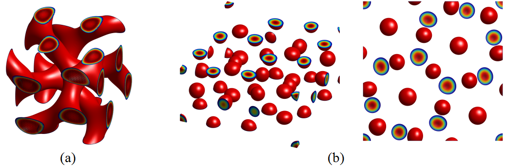
Figure 2: The stationary periodic crystals in LB model. (a) Double gyroid phase with $\xi=0.1,\tau=-2.0,\gamma=2.0$. (b) Sigma phase with $\xi=0.1,\tau=0.01,\gamma=-2.0$ from two perspectives.

Double gyroid

The double gyroid phase is a continuous network periodic phase whose initial values can be chosen as

(74) $$\phi(\bm{r})=\sum_{\bm{h}\in\Lambda_{0}^{DG}}\hat{\phi}(\bm{h})e^{i(\mathbf{B}\bm{h})^{\top}\cdot\bm{r}},$$

where initial lattice points set $\Lambda_{0}^{DG}\subset\mathbb{Z}^{3}$ only on which the Fourier coefficients located are nonzero. The corresponding $\Lambda_{0}^{DG}$ of the double gyroid phase can be found in the Table 1 in [19]. The double gyroid structure belongs to the cubic crystal system, therefore, the $3$-order invertible matrix can be chosen as $\mathbf{B}=(1/\sqrt{6})\mathbf{I}_{3}$. Correspondingly, the computational domain in physical space is $\Omega=[0,2\sqrt{6}\pi)^{3}$. The parameters in LB model Eq. 4 are set as $\xi=0.1,\tau=-2.0,\gamma=2.0$. $128^{3}$ wavefunctions are used in these simulations. Fig. 2 (a) shows the stationary solution of double gyroid profile.

Fig. 3 gives iteration process of the above-mentioned approaches, including the relative energy difference and the gradient changes with iteration, and the CPU time cost. The reference energy value $E_{s}=-12.94291551898271$ is the finally convergent value. As is evident from these results, our AA-BPG methods are most efficient among these approaches under the premise of ensuring energy dissipation. The AA-BPG-4 and AA-BPG-2 approaches have nearly the same numerical behaviors, however, the AA-BPG-4 method spends a little more CPU time than AA-BPG-2 scheme does. The reason is attributed to the cost of solving the subproblem Eq. 22 at each step. For AA-BPG-2 scheme, Eq. 22 can be solved analytically, while for AA-BPG-4 method, Eq. 22 is required to numerically solve a nonlinear system. In Fig. 4, we give the step sizes of AA-BPG-2/4 scheme.

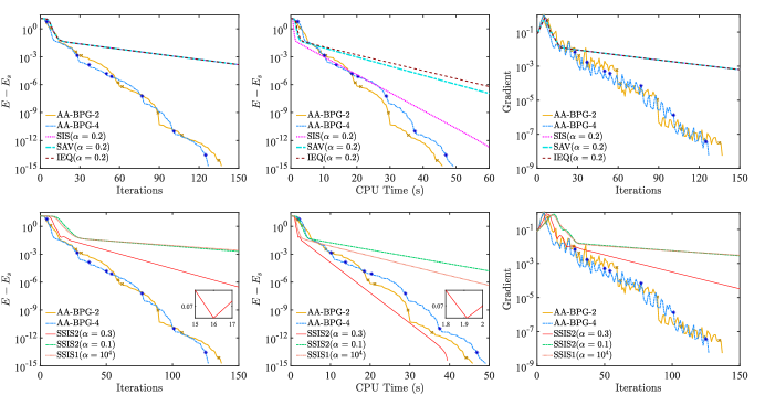
Figure 3: Double gyroid phase: comparisons of numerical behaviors of AA-BPG-2/4 approaches with First row: SIS, SAV and IEQ; Second row: SSIS1 and SSIS2. Left column: Relative energy over iterations; Middle column: Relative energy over CPU times; Right column: Gradient over iterations; The blue and yellow $\times$s mark where restarts occurred.

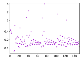
Figure 4: Double gyroid phase: the step sizes of Left: AA-BPG-2; Right: AA-BPG-4 approach.

The SIS, SAV and IEQ approaches have almost the same iterations. Theoretically, the convergence of the SIS is based on the assumption of global Lipschitz constants, while the SAV method always has a modified energy dissipation through adding an arbitrary scaler auxiliary parameter $C$ which guarantees the boundedness of the bulk energy term. The original energy dissipation property of the SAV method depends on the selection of $C$. For computing the double gyroid phase, we find that when $C$ is smaller than $10^{6}$, the SAV scheme cannot keep the original energy dissipation property even if we adopt a small step size $0.001$. Further increasing $C$ to $10^{8}$, we can use a large step size $\alpha=0.2$ to obtain the original energy dissipation feature. Note that there exists a gap between the modified energy and the original energy no matter what the auxiliary parameters are. Like in the SAV method, similar results and phenomena have been also found in the IEQ approach. Among the three methods, the SIS spends the fewest CPU times. The reason is that the SAV and IEQ methods requires to solve a subsystem at each step while the SIS does not.

The SSIS1 is an unconditionally stable scheme through imposing a stabilized term on SIS. Its energy law holds under the assumption of the stabilizing parameter greater than the half of global Lipschitz constant. The step size $\alpha$ can be arbitrary large while the effective step size has a limit. From the numerical results, SSIS1 with $\alpha=10^{4}$ shows a slower convergent rate than the SIS with $\alpha=0.2$ does. An interesting scheme is the conditionally stable SSIS2 proposed in [33] that introduces a center difference stabilizing term to guarantee the second order temporal accuracy. From the point of continuity, the SSIS2 actually adds an inertia term onto the original gradient flow system. The inertia term can accelerate the convergent speed but often accompanied with some oscillations if the step size is large. As Fig. 3 shows, when $\alpha=0.1$ the SSIS2 has almost the same convergent speed with the SSIS1, and holds the energy dissipation property. If increasing $\alpha$, such as $0.3$, the SSIS2 obtains an accelerated speed but with oscillations.

Sigma phase

The second periodic structure considered here is the sigma phase, which is a spherical packed phase recently discovered in block copolymer experiment [23], and the self-consistent mean-field simulation [44]. The sigma phase has a larger, much more complicated tetragonal unit cell with $30$ atoms. For such a pattern, we implement our algorithm on bounded computational domain $\Omega=[0,27.7884)\times[0,27.7884)\times[0,14.1514)$. Correspondingly, the initial values can be found in [44]. When computing the sigma phase, the parameters are set as $\xi=1.0,\tau=0.01,\gamma=2.0$ and $256\times 256\times 128$ wavefunctions are used to discretize LB energy functional. The stationary morphology is shown in Fig. 2 (b). As far as we know, it is the first time to find such complicated sigma phase in such a simple PFC model.

Figure 5: Sigma phase: comparisons of numerical behaviors of the AA-BPG-2/4 approaches with other numerical methods. The information of these plots is the same with Fig. 3.

Fig. 5 compares our proposed methods with other numerical schemes. We still use the reference energy value $E_{s}=-0.93081648457086$ as the baseline to observe the relative energy changes of various numerical approaches. Again, as shown in these results, on the premise of energy dissipation, the new developed gradient based approaches demonstrate a better performance over the existing methods in computing the sigma phase. Among these methods, the AA-BPG-2 method is the most efficient.

6.1.2 Quasicrystals

For the LP free energy Eq. 5, we take the two dimensional dodecagonal quasicrystal as an example to examine the performance of our proposed approach. For dodecagonal quasicrystals, two length scales $q_{1}$ and $q_{2}$ equal to $1$ and $2\cos(\pi/12)$, respectively. Two dimensional dodecagonal quasicrystals can be embedded into four dimensional periodic structures, therefore, the projection method is carried out in four dimensional space. The $4$-order invertible matrix $\mathbf{B}$ associated with to four dimensional periodic structure is chosen as $\mathbf{I}_{4}$. The corresponding computational domain in real space is $[0,2\pi)^{4}$. The projection matrix $\mathcal{P}$ in Eq. Eq. 9 of the dodecagonal quasicrystals is

(75) $$\mathcal{P}=\left(\begin{array}[]{cccc}1&\cos(\pi/6)&\cos(\pi/3)&0\\ 0&\sin(\pi/6)&\sin(\pi/3)&1\end{array}\right).$$

The initial solution is

(76) $$\phi(\bm{r})=\sum_{\bm{h}\in\Lambda^{QC}_{0}}\hat{\phi}(\bm{h})e^{i[(\mathcal{P}\cdot\mathbf{B}\bm{h})^{\top}\cdot\bm{r}]},~{}~{}\bm{r}\in\mathbb{R}^{2},$$

where initial lattice points set $\Lambda_{0}^{QC}\subset\mathbb{Z}^{4}$ can be found in the Table 3 in [20] on which the Fourier coefficients $\hat{\phi}(\bm{h})$ located are nonzero.

Figure 6: The stationary dodecagonal quasicrystal phase in LP model with $c=24,\varepsilon=-6,\kappa=6$. Left: physical morphology; Right: Fourier spectral points whose coefficient intensity is larger than 0.001

The parameters in LP models are set as $c=24,\varepsilon=-6,\kappa=6$, and $38^{4}$ wavefunctions are used to discretize LP energy functional. The convergent stationary quasicrystal is given in Fig. 6, including its order parameter distribution and Fourier spectrum. The numerical behavior of different approaches can be found in Fig. 7. To better observe the change tendency, we use the convergent energy value $E_{s}=-15.97486323815640$ as a baseline to show the relative energy changes against with iterations. We find again that our proposed approaches are more efficient than others.

Figure 7: Dodecagonal quasicrystal: comparisons of numerical behaviors of the AA-BPG-2/4 approaches with other numerical methods. The details of these images are the same with Fig. 3.

6.2 Local acceleration

The motivation of the hybrid method is providing a framework to locally accelerate the existing methods. Certainly, the Newton-PCG method is suitable for all alternative methods mentioned above. In the Fig. 8, we give a detailed comparison of our Newton-PCG method applied to alternative methods. For method M, the acceleration ratio is defined as

(77) $$\text{Acceleration ratio}:=\frac{\text{CPU times of original method M}}{\text{CPU times of hybrid method N-M}}.$$

All numerical parameters, such as step size, of all alternative approaches are keep the same as former to guarantee the best performance. To launch the Newton-PCG method, we choose the gradient difference $\|g_{k}-g_{k-1}\|<10^{-3}$ in computing crystal and energy difference $|E(\hat{\Phi}^{k})-E(\hat{\Phi}^{k-1})|<10^{-4}$ in computing the quasicrystal as the measurement. As shown in our numerical results, our Hessian based methods can accelerate all the existing methods with acceleration ratio ranging from 2-14. After using the proposed local acceleration, we observe that all the compared approaches have similar performance in terms of the CPU time. Moreover, it is noted that the acceleration ratio for the AA-BPG-2 method is the smallest one as is shows the best performance without coupling the Newton-PCG method.

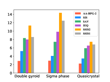
Figure 8: The acceleration ratio of applying Newton-PCG algorithm to existing methods compared with original ones for computing periodic crystals and quasicrystals

7 Conclusion

In this paper, efficient and robust computational approaches have been proposed to find the stationary states of PFC models. Instead of formulating the energy minimization as a gradient flow, we applied the modern optimization methods directly on the discretized energy with mass conservation and energy dissipation. Moreover, the AA-BPG methods with suitable choice of $h$ overcome the global Lipschitz constant requirement in theoretical analysis and the step sizes are adaptively obtained by line search technique. We also propose a practical Newton-PCG method and introduce a hybrid framework to further accelerate the local convergence of gradient based methods. Extensive results in computing periodic crystals and quasicrystals show their advantages in terms of computation efficiency. Thus, it motivates us to continue finding the deep relationship between the gradient flow and the optimization, applying our methods to many related problems, such as SPFC, MPFC models, and extending to more spatial discretization methods.

Appendix A: Proof of 3

Before prove the convergent property, we first present a useful lemma for our analysis.

Lemma 7.1 (Uniformized Kurdyka-Lojasiewicz property [4]).

Let $\Omega$ be a compact set and $E$ is constant on $\Omega$. Then, there exist $\epsilon>0$, $\eta>0$, and $\psi\in\Psi_{\eta}$ such that for all $\bar{u}\in\Omega$ and all $u\in\Gamma_{\eta}(\bar{u},\epsilon)$, one has,

(78) $$\psi^{{}^{\prime}}(E(u)-E(\bar{u}))\mathrm{dist}(\mathbf{0},\partial E(u))\geq 1,$$

where $\Psi_{\eta}=\{\psi\in C[0,\eta)\cap C^{1}(0,\eta),\psi\text{ is concave},\psi(0)=0,\psi^{{}^{\prime}}>0\text{ on }(0,\eta)\}$ and $\Gamma_{\eta}(x,\epsilon)=\{y|\|x-y\|\leq\epsilon,E(x)<E(y)<E(x)+\eta\}$.

Now, we show the proof of 3, which is similar to the framework in [2].

Proof 7.2.

Let $S(x^{0})$ be the set of limiting points of the sequence $\{x^{k}\}_{k=0}^{\infty}$ starting from $x^{0}$. By the boundedness of $\{x^{k}\}_{k=0}^{\infty}$ and the fact $S(x^{0})=\cap_{q\in\mathbb{N}}\overline{\cup_{k\geq q}\{x^{k}\}}$, it follows that $S(x^{0})$ is a non-empty and compact set. Moreover, from Eq. 32, we know $E(x)$ is constant on $S(x^{0})$, denoted by $E^{*}$. If there exists some $k_{0}$ such that $E(x^{k_{0}})=E^{*}$, then we have $E(x^{k})=E^{*}$ for all $k\geq k_{0}$ which is from Eq. 32. In the following proof, we assume that $E(x^{k})>E^{*}$ for all $k$. Therefore, $\forall\epsilon,\eta>0$, there exists some $\ell>0$ such that for all $k>\ell$, we have $\mathrm{dist}(S(x^{0}),x^{k})\leq\epsilon\text{ and }E^{*}<E(x^{k})<E^{*}+\eta$, i.e.

(79) $$x\in\Gamma_{\eta}(x^{*},\epsilon)\quad\text{for all }\quad x^{*}\in S(x^{0}).$$

Applying Lemma 7.1 for all $k>\ell$ we have

$$\psi^{{}^{\prime}}(E(x^{k})-E^{*})\mathrm{dist}(\mathbf{0},E(x^{k}))\geq 1.$$

Form Eq. 34, it implies

(80) $$\psi^{{}^{\prime}}(E(x^{k})-E^{*})\geq\frac{1}{c_{1}(\|x^{k}-x^{k-1}\|+\bar{w}\|x^{k-1}-x^{k-2}\|)}.$$

By the convexity of $\psi$, we have

(81) $$\psi(E(x^{k})-E^{*})-\psi(E(x^{k+1})-E^{*})\geq\psi^{{}^{\prime}}(E(x^{k})-E^{*})(E(x^{k})-E(x^{k+1})).$$

Define $\Delta_{p,q}=\psi(E(x^{p})-E^{*})-\psi(E(x^{q})-E^{*})$ and $C=(1+\bar{w})c_{1}/c_{0}>0$. Together with Eq. 80, Eq. 81 and Eq. 32, we have for all $k>\ell$

(82) $$\Delta_{k,k+1}\geq\frac{c_{0}\|x^{k+1}-x^{k}\|^{2}}{c_{1}(\|x^{k}-x^{k-1}\|+\bar{w}\|x^{k-1}-x^{k-2}\|)}\geq\frac{\|x^{k+1}-x^{k}\|^{2}}{C(\|x^{k}-x^{k-1}\|+\|x^{k-1}-x^{k-2}\|)}.$$

Therefore,

(83) $$2\|x^{k+1}-x^{k}\|\leq\dfrac{1}{2}(\|x^{k}-x^{k-1}\|+\|x^{k-1}-x^{k-2}\|)+2C\Delta_{k,k+1},$$

which is from the geometric inequality. For any $k>\ell$, summing up Eq. 83 for $i=\ell+1,\ldots,k$, it implies

$$\begin{split}&2\sum_{i=\ell+1}^{k}\|x^{i+1}-x^{i}\|\leq{\dfrac{1}{2}}\sum_{i=\ell+1}^{k}(\|x^{i}-x^{i-1}\|+\|x^{i-1}-x^{i-2}\|)+{2C}\sum_{i=\ell+1}^{k}\Delta_{i,i+1}\\ \leq&\sum_{i=\ell+1}^{k}\|x^{i+1}-x^{i}\|+\|x^{\ell+1}-x^{\ell}\|+\|x^{\ell}-x^{\ell-1}\|+2C\Delta_{\ell+1,k+1},\end{split}$$

where the last inequality is from the fact that $\Delta_{p,q}+\Delta_{q,r}=\Delta_{p,r}$ for all $p,q,r\in\mathbb{N}$. Since $\psi\geq 0$, for any $k>\ell$ and we have

(84) $$\begin{split}\sum_{i=\ell+1}^{k}\|x^{i+1}-x^{i}\|\leq\|x^{\ell+1}-x^{\ell}\|+\|x^{\ell}-x^{\ell-1}\|+2C\psi(E(x^{\ell+1})-E^{*}).\end{split}$$

This easily implies that $\sum_{k=1}^{\infty}\|x^{k+1}-x^{k}\|<\infty$. Together with 3, we obtain

$$\lim\limits_{k\rightarrow+\infty}x^{k}=x^{*},\quad\mathbf{0}\in\partial E(x^{*})=0.$$

Appendix B: Proof of Lemma 5.1

The proof is similar to the framework in [47]. Let $x^{*}$ be the exact solution and $e_{i}=x^{*}-x^{i}$ for all $i$. We first prove some important properties of Algorithm 4.

Property I: $r_{i}=Ax^{i}-b$. From the step 4 of Algorithm 4, we have $\alpha_{i}Ap_{i-1}=Ax^{i}-Ax^{i-1}.$ Then,

$$r_{i} =r_{i-1}+\alpha_{i}Ap_{i-1}=r_{0}+\sum_{j=1}^{i}\alpha_{j}Ap_{j-1}=-b+\sum_{j=1}^{i}\alpha_{j}Ap_{j-1}$$

$$=-b+\sum_{j=1}^{i}(Ax^{j}-Ax^{j-1})=-b+Ax^{i}-Ax^{0}=Ax^{i}-b.$$

Property II: $\langle p_{i},b\rangle=\|r_{i}\|_{M^{-1}}^{2}~{}(i=0,1,2,\cdots)$. By the formula (5.40) in  [29], we know that $\langle r_{i},r_{j}\rangle_{M^{-1}}=0~{}(i\neq j)$. Together with the definition of $\beta_{i}$ and $p_{i}$ in Algorithm 4, we get

(85) $$\begin{split}\langle p_{0},b\rangle&=\langle p_{0},-r_{0}\rangle=\langle M^{-1}r_{0},r_{0}\rangle=\|r_{0}\|_{M^{-1}}^{2},\\ \langle p_{i},b\rangle&=\langle p_{i},-r_{0}\rangle=\langle M^{-1}r_{i},r_{0}\rangle+\beta_{i}\langle p_{i-1},-r_{0}\rangle=\beta_{i}\langle p_{i-1},-r_{0}\rangle=\left(\prod_{j=1}^{i}\beta_{i}\right)\langle p_{0},-r_{0}\rangle\\ &=\left(\prod_{j=1}^{i}\beta_{i}\right)\|r_{0}\|_{M^{-1}}^{2}=\left(\prod_{j=2}^{i}\beta_{i}\right)\|r_{1}\|_{M^{-1}}^{2}=\|r_{i}\|_{M^{-1}}^{2},\quad\forall i=1,2,\cdots,\end{split}$$

Property III: $\|e_{i}\|_{A}\geq\|e_{i+1}\|_{A}$. According to the iteration of $p_{i}$, on has

(86) $$\begin{split}\langle p_{i},-r_{i+1}\rangle&=\langle-M^{-1}r_{i}+\beta_{i}p_{i-1},-r_{i+1}\rangle=0+\beta_{i}\langle p_{i-1},-r_{i+1}\rangle\\ &=\left(\prod_{j=1}^{i}\beta_{j}\right)\langle p_{0},-r_{i+1}\rangle=\left(\prod_{j=1}^{i}\beta_{j}\right)\langle M^{-1}r_{0},r_{i+1}\rangle=0.\end{split}$$

By the property I, we have $Ae_{i+1}=A(x^{*}-x^{i+1})=b-Ax^{i+1}=-r_{i+1}$, which implies $\langle p_{i},Ae_{i+1}\rangle=0$. Using the fact that $e_{i}=e_{i+1}+x^{i+1}-x^{i}=e_{i+1}+\alpha_{i+1}p_{i}$, the following equation holds for all $i\geq 0$:

(87) $$\begin{split}\|e_{i}\|_{A}^{2}&=\|e_{i+1}+\alpha_{i+1}p_{i}\|_{A}^{2}=\|e_{i+1}\|_{A}^{2}+2\alpha_{i+1}\langle p_{i},Ae_{i+1}\rangle+\|\alpha_{i+1}p_{i}\|_{A}^{2}\\ &=\|e_{i+1}\|_{A}^{2}+\alpha_{i+1}^{2}\|p_{i}\|_{A}^{2}\geq\|e_{i+1}\|_{A}^{2}.\end{split}$$

Property IV: $\langle x^{i},b\rangle\geq\langle x^{i-1},b\rangle.$ The definition of $\alpha_{j}$ gives $\|r_{j-1}\|_{M^{-1}}^{2}=\alpha_{j}\|p_{j-1}\|_{A}^{2}$. Together with Eq. 85 and Eq. 87, we have

(88) $$\begin{split}\langle x^{i},b\rangle&=\langle x^{i-1},b\rangle+\langle\alpha_{i}p_{i-1},b\rangle=\langle x^{0},b\rangle+\sum_{j=1}^{i}\langle\alpha_{j}p_{j-1},b\rangle=\sum_{j=1}^{i}\alpha_{j}\|r_{j-1}\|_{M^{-1}}^{2}\\ &=\sum_{j=1}^{i}\alpha_{j}^{2}\|p_{j-1}\|_{A}^{2}=\sum_{j=1}^{i}(\|e_{j-1}\|_{A}^{2}-\|e_{j}\|_{A}^{2})=\|e_{0}\|_{A}^{2}-\|e_{i}\|_{A}^{2},\end{split}$$

which implies $\langle x^{i},b\rangle\geq\langle x^{i-1},b\rangle$ by the monotonicity of $\|e_{i}\|_{A}^{2}$.

Now, we can prove the main result. By using the definition of $p_{0}$ and $\alpha_{1}$, we obtain

(89) $$\begin{split}\dfrac{\langle x^{i},b\rangle}{\|b\|^{2}}&\geq\dfrac{\langle x^{1},b\rangle}{\|b\|^{2}}=\dfrac{\langle x^{0}+\alpha_{1}p_{0},b\rangle}{\|b\|^{2}}=\alpha_{1}\dfrac{\langle p_{0},b\rangle}{\|b\|^{2}}=\dfrac{\langle r_{0},p_{0}\rangle}{\langle p_{0},Ap_{0}\rangle}\dfrac{\langle M^{-1}b,b\rangle}{\|b\|^{2}}\\ &=\dfrac{\langle Mp_{0},p_{0}\rangle}{\langle p_{0},Ap_{0}\rangle}\dfrac{\langle M^{-1}b,b\rangle}{\|b\|^{2}}\geq\dfrac{\langle Mp_{0},p_{0}\rangle}{\langle p_{0},Ap_{0}\rangle}\dfrac{1}{\lambda_{\max}(M)}.\end{split}$$

Since $M$ is positive, we know $M=M^{1/2}M^{1/2}$, where $M^{1/2}$ is still positive. As a result,

(90) $$\|M\|=\lambda_{max}(M)=\lambda_{\max}(M^{1/2}M^{1/2})=\lambda^{2}_{\max}(M^{1/2})=\|M^{1/2}\|^{2}.$$

Let $y=M^{1/2}p_{0}$, we get

(91) $$\begin{split}\dfrac{\langle Mp_{0},p_{0}\rangle}{\langle p_{0},Ap_{0}\rangle}&=\dfrac{\langle y,y\rangle}{\langle y,M^{-1/2}AM^{-1/2}y\rangle}\geq\dfrac{1}{\lambda_{\max}(M^{-1/2}AM^{-1/2})}=\dfrac{1}{\|M^{-1/2}AM^{-1/2}\|}\\ &\geq\dfrac{1}{\|M^{-1/2}\|\cdot\|A\|\cdot\|M^{-1/2}\|}=\dfrac{\|M\|}{\|A\|}=\dfrac{\lambda_{\max}(M)}{\lambda_{\max}(A)}.\end{split}$$

where the second inequality takes the fact that $\|AB\|\leq\|A\|\cdot\|B\|$. Together with Eq. 89, we get

(92) $$\dfrac{\langle x^{i},b\rangle}{\|b\|^{2}}\geq\dfrac{\langle Mp_{0},p_{0}\rangle}{\langle p_{0},Ap_{0}\rangle}\dfrac{1}{\lambda_{\max}(M)}\geq\dfrac{\lambda_{\max}(M)}{\lambda_{\max}(A)}\dfrac{1}{\lambda_{\max}(M)}=\dfrac{1}{\lambda_{\max}(A)}.$$

To verify another inequality, we use Eq. 88 and the fact that $e_{0}=x^{*}-x^{0}=-A^{-1}b$,

$$\dfrac{\langle x^{i},b\rangle}{\|b\|^{2}}\ =\dfrac{\|e_{0}\|_{A}^{2}-\|e_{i}\|_{A}^{2}}{\|b\|^{2}}\leq\dfrac{\|e_{0}\|_{A}^{2}}{\|b\|^{2}}=\dfrac{\|A^{-1}b\|_{A}^{2}}{\|b\|^{2}}=\dfrac{\langle b,A^{-1}b\rangle}{\|b\|^{2}}\leq\dfrac{1}{\lambda_{\min}(A)}.$$

References

- [1] J. Barzilai and J. M. Borwein, Two-point step size gradient methods, IMA journal of numerical analysis, 8 (1988), pp. 141–148.
- [2] H. H. Bauschke, J. Bolte, and M. Teboulle, A descent lemma beyond lipschitz gradient continuity: first-order methods revisited and applications, Mathematics of Operations Research, 42 (2017), pp. 330–348.
- [3] A. Beck and M. Teboulle, A fast iterative shrinkage-thresholding algorithm for linear inverse problems, SIAM journal on imaging sciences, 2 (2009), pp. 183–202.
- [4] J. Bolte, S. Sabach, and M. Teboulle, Proximal alternating linearized minimization for nonconvex and nonsmooth problems, Mathematical Programming, 146 (2014), pp. 459–494.
- [5] J. Bolte, S. Sabach, M. Teboulle, and Y. Vaisbourd, First order methods beyond convexity and lipschitz gradient continuity with applications to quadratic inverse problems, SIAM Journal on Optimization, 28 (2018), pp. 2131–2151.
- [6] S. Brazovskii, Phase transition of an isotropic system to a nonuniform state, Soviet Journal of Experimental and Theoretical Physics, 41 (1975), p. 85.
- [7] L. M. Bregman, The relaxation method of finding the common point of convex sets and its application to the solution of problems in convex programming, USSR computational mathematics and mathematical physics, 7 (1967), pp. 200–217.
- [8] H. Brezis, Functional analysis, Sobolev spaces and partial differential equations, Springer Science & Business Media, 2010.
- [9] L. Chen, Phase-field models for microstructure evolution, Annual review of materials research, 32 (2002), pp. 113–140.
- [10] L. Q. Chen and J. Shen, Applications of semi-implicit fourier-spectral method to phase field equations, Computer Physics Communications, 108 (1998), pp. 147–158.
- [11] K. Cheng, C. Wang, and S. M. Wise, An energy stable bdf2 fourier pseudo-spectral numerical scheme for the square phase field crystal equation, Communications in Computational Physics, 26 (2019), pp. 1335–1364.
- [12] Q. Du and J. Zhang, Adaptive finite element method for a phase field bending elasticity model of vesicle membrane deformations, SIAM Journal on Scientific Computing, 30 (2008), pp. 1634–1657.
- [13] Q. Du and W.-x. Zhu, Stability analysis and application of the exponential time differencing schemes, Journal of Computational Mathematics, (2004), pp. 200–209.
- [14] X. Feng, Y. He, and C. Liu, Analysis of finite element approximations of a phase field model for two-phase fluids, Mathematics of computation, 76 (2007), pp. 539–571.
- [15] R. Guo and Y. Xu, A high order adaptive time-stepping strategy and local discontinuous galerkin method for the modified phase field crystal equation, Comput. Phys, 24 (2018), pp. 123–151.
- [16] H. Hiller, The crystallographic restriction in higher dimensions, Acta Crystallographica Section A: Foundations of Crystallography, 41 (1985), pp. 541–544.
- [17] Z. Hu, S. M. Wise, C. Wang, and J. S. Lowengrub, Stable and efficient finite-difference nonlinear-multigrid schemes for the phase field crystal equation, Journal of Computational Physics, 228 (2009), pp. 5323–5339.
- [18] K. Jiang, J. Tong, P. Zhang, and A.-C. Shi, Stability of two-dimensional soft quasicrystals in systems with two length scales, Physical Review E, 92 (2015), p. 042159.
- [19] K. Jiang, C. Wang, Y. Huang, and P. Zhang, Discovery of new metastable patterns in diblock copolymers, Communications in Computational Physics, 14 (2013), pp. 443–460.
- [20] K. Jiang and P. Zhang, Numerical methods for quasicrystals, Journal of Computational Physics, 256 (2014), pp. 428–440.
- [21] Y. Katznelson, An introduction to harmonic analysis, 2004.
- [22] H. G. Lee, J. Shin, and J.-Y. Lee, First-and second-order energy stable methods for the modified phase field crystal equation, Computer Methods in Applied Mechanics and Engineering, 321 (2017), pp. 1–17.
- [23] S. Lee, M. Bluemle, and F. Bates, Discovery of a frank-kasper phase in sphere-forming block copolymer melts, Science, 330 (2010), p. 349.
- [24] Q. Li, Z. Zhu, G. Tang, and M. B. Wakin, Provable bregman-divergence based methods for nonconvex and non-lipschitz problems, arXiv preprint arXiv:1904.09712, (2019).
- [25] R. Lifshitz and H. Diamant, Soft quasicrystals–why are they stable?, Philosophical Magazine, 87 (2007), pp. 3021–3030.
- [26] R. Lifshitz and D. Petrich, Theoretical model for faraday waves with multiple-frequency forcing, Physical review letters, 79 (1997), pp. 1261–1264.
- [27] X. Liu, Z. Wen, X. Wang, M. Ulbrich, and Y. Yuan, On the analysis of the discretized kohn–sham density functional theory, SIAM Journal on Numerical Analysis, 53 (2015), pp. 1758–1785.
- [28] S. K. Mkhonta, K. R. Elder, and Z.-F. Huang, Exploring the complex world of two-dimensional ordering with three modes, Phys. Rev. Lett., 111 (2013), p. 035501, https://doi.org/10.1103/PhysRevLett.111.035501, https://link.aps.org/doi/10.1103/PhysRevLett.111.035501.
- [29] J. Necedal and S. J.Wright, Numerical Optimization, Springer, 2006.
- [30] B. O’donoghue and E. Candes, Adaptive restart for accelerated gradient schemes, Foundations of computational mathematics, 15 (2015), pp. 715–732.
- [31] N. Provatas and K. Elder, Phase-field methods in materials science and engineering, Wiley-VCH, 2010.
- [32] J. Shen, J. Xu, and J. Yang, A new class of efficient and robust energy stable schemes for gradient flows, SIAM Review, 61 (2019), pp. 474–506.
- [33] J. Shen and X. Yang, Numerical approximations of allen-cahn and cahn-hilliard equations, Discrete Contin. Dyn. Syst, 28 (2010), pp. 1669–1691.
- [34] A.-C. Shi, J. Noolandi, and R. C. Desai, Theory of anisotropic fluctuations in ordered block copolymer phases, Macromolecules, 29 (1996), pp. 6487–6504.
- [35] J. Shin, H. G. Lee, and J.-Y. Lee, First and second order numerical methods based on a new convex splitting for phase-field crystal equation, Journal of Computational Physics, 327 (2016), pp. 519–542.
- [36] J. Swift and P. C. Hohenberg, Hydrodynamic fluctuations at the convective instability, Phys. Rev. A, 15 (1977), pp. 319–328, https://doi.org/10.1103/PhysRevA.15.319, http://link.aps.org/doi/10.1103/PhysRevA.15.319.
- [37] P. Tseng, On accelerated proximal gradient methods for convex-concave optimization, submitted to SIAM Journal on Optimization, 2 (2008), p. 3.
- [38] M. Ulbrich, Z. Wen, C. Yang, D. Klockner, and Z. Lu, A proximal gradient method for ensemble density functional theory, SIAM Journal on Scientific Computing, 37 (2015), pp. A1975–A2002.
- [39] J. Van Tiel, Convex analysis: An introductory text, 1984.
- [40] C. Wang and S. M. Wise, An energy stable and convergent finite-difference scheme for the modified phase field crystal equation, SIAM Journal on Numerical Analysis, 49 (2011), pp. 945–969.
- [41] S. M. Wise, C. Wang, and J. S. Lowengrub, An energy-stable and convergent finite-difference scheme for the phase field crystal equation, SIAM Journal on Numerical Analysis, 47 (2009), p. 2269.
- [42] X. Wu, Z. Wen, and W. Bao, A regularized newton method for computing ground states of bose–einstein condensates, Journal of Scientific Computing, 73 (2017), pp. 303–329.
- [43] X. Xiao, Y. Li, Z. Wen, and L. Zhang, A regularized semi-smooth newton method with projection steps for composite convex programs, Journal of Scientific Computing, 76 (2018), pp. 364–389.
- [44] N. Xie, W. Li, F. Qiu, and A.-C. Shi, phase formed in conformationally asymmetric ab-type block copolymers, Acs Macro Letters, 3 (2014), pp. 906–910.
- [45] C. Xu and T. Tang, Stability analysis of large time-stepping methods for epitaxial growth models, SIAM Journal on Numerical Analysis, 44 (2006), pp. 1759–1779.
- [46] X. Yang, Linear, first and second-order, unconditionally energy stable numerical schemes for the phase field model of homopolymer blends, Journal of Computational Physics, 327 (2016), pp. 294–316.
- [47] X.-Y. Zhao, D. Sun, and K.-C. Toh, A newton-cg augmented lagrangian method for semidefinite programming, SIAM Journal on Optimization, 20 (2010), pp. 1737–1765.