New features in the JHU generator framework: Constraining Higgs boson properties from on-shell and off-shell production

Abstract

We present an extension of the JHUGen and MELA framework, which includes an event generator and library for the matrix element analysis. It enables simulation, optimal discrimination, reweighting techniques, and analysis of a bosonic resonance and the triple and quartic gauge boson interactions with the most general anomalous couplings. The new features, which become especially relevant at the current stage of LHC data taking, are the simulation of gluon fusion and vector boson fusion in the off-shell region, associated $ZH$ production at NLO QCD including the $gg$ initial state, and the simulation of a second spin-zero resonance. We also quote translations of the anomalous coupling measurements into constraints on dimension-six operators of an effective field theory. Some of the new features are illustrated with projections for experimental measurements with the full LHC and HL-LHC datasets.

I Introduction

We present a coherent framework for the measurement of couplings of the Higgs ($H$) boson and a possible second spin-zero resonance. Our framework includes a Monte Carlo generator and matrix element techniques for optimal analysis of the data. We build upon the earlier developed framework of the JHU generator and MELA analysis package Gao:2010qx ; Bolognesi:2012mm ; Anderson:2013afp ; Gritsan:2016hjl and extensively use matrix elements provided by MCFM Campbell:2010ff ; Campbell:2011bn ; Campbell:2013una ; Campbell:2015vwa ; Campbell:2015qma . Thanks to the transparent implementation of standard model (SM) processes in MCFM, we extend them to add the most general scalar and gauge couplings and possible additional states. This allows us to build on the previously studied topics Nelson:1986ki ; Soni:1993jc ; Plehn:2001nj ; Choi:2002jk ; Buszello:2002uu ; Hankele:2006ma ; Accomando:2006ga ; Godbole:2007cn ; Hagiwara:2009wt ; Gao:2010qx ; DeRujula:2010ys ; Christensen:2010pf ; Bolognesi:2012mm ; Ellis:2012xd ; Chen:2012jy ; Artoisenet:2013puc ; Anderson:2013afp ; Chen:2013waa ; Maltoni:2013sma ; Azatov:2014jga ; Cacciapaglia:2014rla ; Denner:2014cla ; Dolan:2014upa ; Englert:2014ffa ; Gonzalez-Alonso:2014eva ; Ballestrero:2015jca ; Greljo:2015sla ; Hespel:2015zea ; Kauer:2015dma ; Kauer:2015hia ; Kilian:2015opv ; Mimasu:2015nqa ; Degrande:2016dqg ; Dwivedi:2016xwm ; Gritsan:2016hjl ; deFlorian:2016spz ; Azatov:2016xik ; Denner:2017vms ; Deutschmann:2017qum ; Greljo:2017spw ; Goncalves:2017gzy ; Jager:2017owh ; Brass:2018hfw ; Gomez-Ambrosio:2018pnl ; Goncalves:2018pkt ; Harlander:2018yns ; Harlander:2018yio ; Lee:2018fxj ; Kalinowski:2018oxd ; Perez:2018kav ; Jaquier:2019bfs ; Denner:2019fcr ; Banerjee:2019twi and present phenomenological results in a unified approach. This framework includes many options for production and decay of the $H$ boson. Here we consider gluon fusion (ggH), vector boson fusion (VBF), and associated production with a vector boson ($VH$) in both on-shell $H$ and off-shell $H^{*}$ production, with decays to two vector bosons. In the off-shell case, interference with background processes is included. Additional heavy particles in the gluon fusion loop and a second resonance interfering with the SM processes are also considered. In the $VH$ process, we include next-to-leading order QCD corrections, as well as the gluon fusion process for $ZH$. The processes with direct sensitivity to fermion $H\!f\!\bar{f}$ couplings, such as $t\bar{t}H$, $b\bar{b}H$, $tqH$, or $H\to\tau^{+}\tau^{-}$, are discussed in Ref. Gritsan:2016hjl .

In an earlier version of our framework, we focused mostly on the Run-I targets and their possible extensions as documented in Refs. Gao:2010qx ; Bolognesi:2012mm ; Anderson:2013afp . It was adopted in Run-I analyses using Large Hadron Collider (LHC) data Chatrchyan:2012xdj ; Chatrchyan:2012jja ; Chatrchyan:2013mxa ; Chatrchyan:2013iaa ; Aad:2013xqa ; Khachatryan:2014iha ; Khachatryan:2014ira ; Khachatryan:2014kca ; Khachatryan:2015mma ; Khachatryan:2015cwa ; Aad:2015mxa ; Khachatryan:2016tnr . Some new features in this framework have been reported earlier deFlorian:2016spz and have been used for LHC experimental analyses. Most notably, this framework was employed in recent Run-II measurements of the $HVV$ anomalous couplings from the first joint analysis of on-shell production and decay Sirunyan:2017tqd ; Sirunyan:2019nbs , from the first joint analysis of on-shell and off-shell $H$ boson production Sirunyan:2019twz , for the first measurement of the CP structure of the Yukawa interaction between the $H$ boson and top quark Sirunyan:2020sum , in the search for a second resonance in interference with the continuum background Sirunyan:2018qlb ; Sirunyan:2019pqw , and in projections to future on-shell and off-shell $H$ boson measurements at the High Luminosity (HL) LHC Cepeda:2019klc . In this paper, we document, review, and highlight the new features critical for exploring the full Run-II dataset at the LHC and preparing for Run-III and the HL-LHC. We also broaden the theoretical underpinning, allowing interpretation in terms of either anomalous couplings or an effective field theory (EFT) framework.

Both Run-I and Run-II of the LHC have provided a large amount of data on $H$ boson properties and its interactions with other SM particles, as analyzed by the ATLAS and CMS experiments. The $H$ boson has been observed in all accessible production channels, gluon fusion, weak vector boson fusion, $VH$ associated production, and top-quark associated production Khachatryan:2016vau ; Sirunyan:2018koj ; Aad:2019mbh ; Sirunyan:2018kst ; Aaboud:2018zhk ; Sirunyan:2018hoz ; Aaboud:2018urx , and its production strength is consistent with the SM prediction within the uncertainties deFlorian:2016spz . Also its decay channels into gauge bosons ($ZZ,WW,\gamma\gamma)$ have been observed and do not show significant deviations within the uncertainties  Khachatryan:2016vau ; Sirunyan:2018koj ; Aad:2019mbh . The fermionic interactions have been established for the third generation quarks ($t,b$) and the $\tau$ lepton Sirunyan:2018kst ; Aaboud:2018zhk ; Sirunyan:2018hoz ; Aaboud:2018urx ; Sirunyan:2017khh ; Aaboud:2018pen , and so far, they are consistent with the SM within the uncertainties.

While this picture shows that Nature does not radically deviate from the SM dynamics, it should be noted that many generic extensions of the SM predict deviations only below the current precision. Open questions remain, for example about CP-odd mixtures, the Yukawa coupling hierarchy, and other states involved in electroweak symmetry breaking. These questions can be addressed in the years to come by fully utilizing the existing and upcoming LHC data sets. In particular, the study of kinematic tails of distributions involving the $H$ boson is becoming accessible for the first time. These signals involve off-shell $H$ boson production and strong interference effects with irreducible backgrounds that are subject to the electroweak unitarization mechanism in the SM. This feature turns the kinematic tails into particularly sensitive probes of the mechanism of electroweak symmetry breaking and possible extensions beyond the SM. Moreover, the study of electroweak production of the $H$ boson (VBF and $VH$) is probing $HVV$ interactions over a large range of momentum transfer, which can expose possible new particles that couple through loops. Even the direct production of new resonances will first show up as deviations from the expected high-energy tail of kinematic distributions. Hence, analyzing these newly accessible features in off-shell $H$ boson production is of paramount importance to understand electroweak symmetry breaking in the SM and possible extensions involving new particles. In the following, we review the framework and demonstrate its capabilities through examples of possible analyses. The technical details of the framework are described in the manual, which can be downloaded at jhugen , together with the source code.

II Parameterization of anomalous interactions

II.1 $H$ boson interactions

We present our parameterization of anomalous couplings relevant for on-shell and off-shell $H$ boson production and decay.

(a) $HVV$

(b) $Hf\bar{f}$

(c) $HVf\bar{f}$

(d) $Hf\bar{f}f\bar{f}$

Figure 1: Vertices relevant for $HVV$ and $H\!f\!\bar{f}$ interactions.

Following the notation of Refs. Gao:2010qx ; Bolognesi:2012mm ; Anderson:2013afp , the $HVV$ scattering amplitude of a spin-zero boson $H$ and two vector bosons $VV$ with polarization vectors and momenta $\varepsilon_{1}^{\mu}$, $q_{1}$ and $\varepsilon_{2}^{\mu}$, $q_{2}$, as illustrated in Fig. 1(a), is parameterized by

$$A({HV_{1}V_{2}})\!=\!\frac{1}{v} \bigg{\{} M_{V_{1}}^{2}\bigg{(}g_{1}^{VV}+\frac{\kappa_{1}^{VV}q_{1}^{2}+\kappa_{2}^{VV}q_{2}^{2}}{\left(\Lambda_{1}^{VV}\right)^{2}}+\frac{\kappa_{3}^{VV}(q_{1}+q_{2})^{2}}{\left(\Lambda_{Q}^{VV}\right)^{2}}+\frac{2q_{1}\cdot q_{2}}{M_{V_{1}}^{2}}g_{2}^{VV}\bigg{)}(\varepsilon_{1}\cdot\varepsilon_{2})$$ (1)

$$-2g_{2}^{VV}\,{(\varepsilon_{1}\cdot q_{2})(\varepsilon_{2}\cdot q_{1})}-2g_{4}^{VV}\,{\varepsilon_{\varepsilon_{1}\,\varepsilon_{2}\,q_{1}\,q_{2}}}\bigg{\}}\,,$$

where $M_{V_{1}}$ is the vector boson’s pole mass, $v$ is the SM Higgs field vacuum expectation value, and $g_{1,2,4}^{VV}$, $\kappa_{1,2}^{VV}/(\Lambda_{1}^{VV})^{2}$, and $\kappa_{3}^{VV}/(\Lambda_{Q}^{VV})^{2}$ are coupling constants to be measured from data. This parametrization represents the most general Lorentz-invariant form.

At tree level in the SM, only the CP-even $HZZ$ and $HWW$ interactions contribute via $g_{1}^{ZZ}=g_{1}^{WW}=2$. The loop-induced interactions of $HZ\gamma$, $H\gamma\gamma$, and $Hgg$ contribute effectively via the CP-even $g_{2}^{VV}$ terms and are parameterically suppressed by $\alpha$ or $\alpha_{s}$. The CP-violating couplings $g_{4}^{VV}$ are generated only at three-loop level in the SM and are therefore tiny. Beyond the SM, all of these couplings can receive additional contributions, which do not necessarily have to be small. For example, the $Hgg$ interaction can be parameterized through a fermion loop, as discussed later in application to Eq. (37). The fermions in the loop interact with the $H$ boson as illustrated in Fig. 1(b), with the couplings $\kappa_{f}$ and $\tilde{\kappa}_{f}$ and the amplitude

$${A}(H\!f\!\bar{f})=-\frac{m_{f}}{v}\bar{\psi}_{f}\left(\kappa_{f}+\mathrm{i}\,\tilde{\kappa}_{f}\gamma_{5}\right){\psi}_{f}\,,$$ (2)

where $\bar{\psi}_{f}$ and ${\psi}_{f}$ are the Dirac spinors and $m_{f}$ is the fermion mass. One may equivalently choose to express the couplings through a Lagrangian (up to an unphysical global phase)

$${\cal L}_{hff}=-\frac{m_{f}}{v}\bar{\psi}_{f}\left(\kappa_{f}+\mathrm{i}\,\tilde{\kappa}_{f}\gamma_{5}\right)\psi_{f}\,h\,,$$ (3)

which allows a connection to be made between the couplings $\kappa_{f}$ and $\tilde{\kappa}_{f}$ and anomalous operators in an effective field theory. In the SM, the dominant contribution to gluon fusion comes from a top quark loop with $(\kappa_{t},\tilde{\kappa}_{t})=(1,0)$.

The couplings $\kappa_{i}^{VV}/(\Lambda_{i}^{VV})^{2}$ in Eq. (1) are introduced to allow for additional momentum dependence. Below, we also show that these terms can be reinterpreted as the contact interactions shown in Figs. 1(c) and 1(d). By symmetry we have $\kappa_{1}^{ZZ}=\kappa_{2}^{ZZ}$, but we do not enforce $\kappa_{1}^{WW}=\kappa_{2}^{WW}$ for $W^{\pm}$ bosons. Note that $\kappa_{1}^{\gamma\gamma}=\kappa_{2}^{\gamma\gamma}=\kappa_{1}^{gg}=\kappa_{2}^{gg}=\kappa_{1}^{Z\gamma}=0$, while $\kappa_{1}^{\gamma Z}=\kappa_{2}^{Z\gamma}$ may contribute Khachatryan:2014kca . The coupling $\kappa_{3}^{VV}/(\Lambda_{Q}^{VV})^{2}$ allows for scenarios which violate the gauge symmetries of the SM.

For the $Hgg$ couplings entering the gluon fusion process we also consider the full one-loop dependence instead of the effective $g_{2,4}^{gg}$ couplings in Eq. (1). This feature is important for correctly describing off-shell Higgs production and additional broad, heavy resonances, where the $q^{2}$-dependence of the interaction cannot be approximated as a constant coupling. In addition to the closed quark loop with explicit dependence on the bottom and top quark masses, we allow for the insertion of fourth generation $b^{\prime}$ and $t^{\prime}$ quarks into the loop.

If a gauge boson in Eq. (1) is coupled to a light fermion current, we replace its polarization vectors by

$$\varepsilon_{i}^{\mu}(q_{i})\to j^{\mu}_{i}=e\,\frac{\bar{\psi}_{f^{\prime}}\gamma^{\mu}\left(g^{Vf^{\prime}f}_{\mathrm{L}}\,\omega_{\mathrm{L}}+g^{Vf^{\prime}f}_{\mathrm{R}}\,\omega_{\mathrm{R}}\right)\psi_{f}}{q_{i}^{2}-M_{V}^{2}+\mathrm{i}M_{V}\Gamma_{V}}\,,$$ (4)

where $e$ is the electron electric charge, $\Gamma_{V}$ is the gauge boson’s width, $\omega_{\mathrm{L,R}}$ are the left- and right-handed chirality projectors, and the $g^{Vf^{\prime}f}_{\mathrm{L,R}}$ are the corresponding couplings of the gauge boson $V$ to fermions. We also allow for exchanges of additional spin-1 bosons $V^{\prime}$ between the $H$ boson and the fermions. Hence, we add

$$\varepsilon_{i}^{\mu}(q_{i})\to j^{\mu}_{i}-\,\frac{\bar{\psi}_{f^{\prime}}\gamma^{\mu}\left(e_{\mathrm{L}}^{V^{\prime}f^{\prime}f}\omega_{\mathrm{L}}+e_{\mathrm{R}}^{V^{\prime}f^{\prime}f}\omega_{\mathrm{R}}\right)\psi_{f}}{q_{i}^{2}-M_{V^{\prime}}^{2}+\mathrm{i}M_{V^{\prime}}\Gamma_{V^{\prime}}}\,,$$ (5)

with the chirality and flavor dependent couplings $e_{\mathrm{L,R}}^{V^{\prime}f^{\prime}f}$. In this approach, we allow for flavor changing interactions ($f^{\prime}\neq f$) in both the neutral and charged $V^{\prime}$ interactions. In the case where the $V^{\prime}$ boson is very heavy, the limit $M_{V^{\prime}}^{2}/q_{i}^{2}\to\infty$ yields the contact interaction

$$\varepsilon_{i}^{\mu}(q_{i})\to j^{\mu}_{i}+\frac{1}{M_{V^{\prime}}^{2}}\;{\bar{\psi}_{f^{\prime}}\gamma^{\mu}\left(e_{\mathrm{L}}^{V^{\prime}f^{\prime}f}\omega_{\mathrm{L}}+e_{\mathrm{R}}^{V^{\prime}f^{\prime}f}\omega_{\mathrm{R}}\right)\psi_{f}}$$ (6)

in Fig. 1(c-d). We note that these contact terms and new $V^{\prime}$ states are not the primary interest in this study because their existence would become evident in resonance searches and in electroweak measurements, without the need for $H$ boson production. Moreover, the $HZf{\bar{f}}$ contact terms are equivalent to the already constrained $\kappa_{1,2}^{ZZ}$ and $\kappa_{2}^{Z\gamma}$ terms Gonzalez-Alonso:2014eva ; Greljo:2015sla if coupling flavor universality is assumed. Under the approximation that the $Z$ boson has a narrow width, this correspondence, given in Eq. (28), only involves real couplings. For example, in the limit where $\Gamma_{Z}\ll M_{Z}$, a nonzero $\kappa_{1}^{ZZ}/(\Lambda_{1}^{ZZ})^{2}$ in Eq. (1) is equivalent to shifting $g_{1}^{ZZ}\to g_{1}^{ZZ}+2\kappa_{1}^{ZZ}(M_{Z}\big{/}\Lambda_{1}^{ZZ})^{2}$ and activating a contact interaction $g_{1}^{ZZ^{\prime}}=\kappa_{1}^{ZZ}(M_{Z^{\prime}}\big{/}\Lambda_{1}^{ZZ})^{2}$, $e^{Z^{\prime}f^{\prime}f}_{\lambda}=e\,g_{\lambda}^{Zf^{\prime}f}$.

The parameterization of the amplitude in Eq. (1) can be related to a fundamental Lagrange density function. Here, we closely follow the so-called Higgs basis of Ref. deFlorian:2016spz , which is based on an effective field theory expansion up to dimension six. The relevant $\mathrm{SU(3)\times SU(2)\times U(1)}$ invariant Lagrangian for $H$ boson interactions with gauge bosons (in the mass eigenstate parameterization) reads

$${\cal L}_{\rm hvv}= {h\over v}\left[\left(1+\delta c_{z}\right){(g^{2}+g^{\prime 2})v^{2}\over 4}Z_{\mu}Z_{\mu}+c_{zz}{g^{2}+g^{\prime}{}^{2}\over 4}Z_{\mu\nu}Z_{\mu\nu}+c_{z\Box}g^{2}Z_{\mu}\partial_{\nu}Z_{\mu\nu}+\tilde{c}_{zz}{g^{2}+g^{\prime}{}^{2}\over 4}Z_{\mu\nu}\tilde{Z}_{\mu\nu}\right.$$ (7)

$$\left.+\left(1+\delta c_{w}\right){g^{2}v^{2}\over 2}W_{\mu}^{+}W_{\mu}^{-}+c_{ww}{g^{2}\over 2}W_{\mu\nu}^{+}W_{\mu\nu}^{-}+c_{w\Box}g^{2}\left(W_{\mu}^{-}\partial_{\nu}W_{\mu\nu}^{+}+{\mathrm{h}.c.}\right)+\tilde{c}_{ww}{g^{2}\over 2}W_{\mu\nu}^{+}\tilde{W}_{\mu\nu}^{-}\right.$$

$$\left.+c_{z\gamma}{e\sqrt{g^{2}+g^{\prime}{}^{2}}\over 2}Z_{\mu\nu}A_{\mu\nu}+\tilde{c}_{z\gamma}{e\sqrt{g^{2}+g^{\prime}{}^{2}}\over 2}Z_{\mu\nu}\tilde{A}_{\mu\nu}+c_{\gamma\Box}gg^{\prime}Z_{\mu}\partial_{\nu}A_{\mu\nu}\right.$$

$$\left.+c_{\gamma\gamma}{e^{2}\over 4}A_{\mu\nu}A_{\mu\nu}+\tilde{c}_{\gamma\gamma}{e^{2}\over 4}A_{\mu\nu}\tilde{A}_{\mu\nu}+c_{gg}{g_{s}^{2}\over 4}G_{\mu\nu}^{a}G_{\mu\nu}^{a}+\tilde{c}_{gg}{g_{s}^{2}\over 4}G_{\mu\nu}^{a}\tilde{G}_{\mu\nu}^{a}\right]\,,$$

in accordance with Eq. (II.2.20) in Ref. deFlorian:2016spz . The fields and real-valued couplings, as well as the corresponding dimension-six operators, are defined in Ref. deFlorian:2016spz ; for example, $g^{2}+g^{\prime 2}=e^{2}/(s_{w}c_{w})^{2}$, $e^{2}=4\pi\alpha$ and $g_{s}^{2}=4\pi\alpha_{s}$. We note that when restricting the discussion to the dimension-six effective field theory (see Eq. (II.2.38) in Ref. deFlorian:2016spz ), Eq. (7) is parameterized by ten real degrees of freedom, so not all of the coefficients are independent. For example, the coefficients $\delta c_{w}$, $c_{ww}$, $\tilde{c}_{ww}$, $c_{w\Box}$, and $c_{\gamma\Box}$ can be expressed through linear combinations of the other couplings. The redundancy was introduced intentionally in Ref. deFlorian:2016spz for easier connections to observable quantities in Higgs physics.

The generality of our amplitude parameterization allows us to uniquely represent each EFT coefficient in Eq. (7) by an anomalous coupling in Eq. (1). Limiting our couplings to real-valued numbers, we find

$$\delta c_{z}=\frac{1}{2}g_{1}^{ZZ}-1\,,\quad\quad c_{zz}=-\frac{2s_{w}^{2}c_{w}^{2}}{e^{2}}g_{2}^{ZZ}\,,\quad\quad c_{z\Box}=\frac{M_{Z}^{2}s_{w}^{2}}{e^{2}}\,\frac{\kappa_{1}^{ZZ}}{(\Lambda_{1}^{ZZ})^{2}}\,,\quad\quad\tilde{c}_{zz}=-\frac{2s_{w}^{2}c_{w}^{2}}{e^{2}}g_{4}^{ZZ}\,,$$

$$\delta c_{w}=\frac{1}{2}g_{1}^{WW}-1\,,\quad\quad c_{ww}=-\frac{2s_{w}^{2}}{e^{2}}g_{2}^{WW}\,,\quad\quad c_{w\Box}=\frac{M_{W}^{2}s_{w}^{2}}{e^{2}}\,\frac{\kappa_{1}^{WW}}{(\Lambda_{1}^{WW})^{2}}\,,\quad\quad\tilde{c}_{ww}=-\frac{2s_{w}^{2}}{e^{2}}g_{4}^{WW}\,,$$

$$c_{z\gamma}=-\frac{2s_{w}c_{w}}{e^{2}}g_{2}^{Z\gamma}\,,\quad\quad\tilde{c}_{z\gamma}=-\frac{2s_{w}c_{w}}{e^{2}}g_{4}^{Z\gamma}\,,\quad\quad c_{\gamma\Box}=\frac{s_{w}c_{w}}{e^{2}}\,\frac{M_{Z}^{2}}{(\Lambda_{1}^{Z\gamma})^{2}}\kappa_{2}^{Z\gamma}\,,$$

$$c_{\gamma\gamma}=-\frac{2}{e^{2}}g_{2}^{\gamma\gamma}\,,\quad\quad\tilde{c}_{\gamma\gamma}=-\frac{2}{e^{2}}g_{4}^{\gamma\gamma}\,,\quad\quad c_{gg}=-\frac{2}{g_{s}^{2}}g_{2}^{gg}\,,\quad\quad\tilde{c}_{gg}=-\frac{2}{g_{s}^{2}}g_{4}^{gg}\,.$$ (8)

The Lagrangian for SM $HVV$ interactions is retained by setting $\delta c_{z}=\delta c_{w}=0$ and all other $c_{i}=0$. Hence, only the CP-even $HZZ$ and $HWW$ interactions remain at tree level.

Not every anomalous coupling in Eq. (1) has a corresponding term in the EFT Lagrangian of Eq. (7). For example, the gauge invariance violating term $\kappa_{3}^{VV}/(\Lambda_{Q}^{VV})^{2}$ has no correspondence because ${\cal L}_{\rm hvv}$ is gauge invariant by construction. Similarly, charge symmetry in ${\cal L}_{\mathrm{hvv}}$ enforces $\kappa_{1}^{WW}=\kappa_{2}^{WW}$, which does not necessarily have to be true in our amplitude setting. For a unique comparison at the level of dimension-six interactions, the above mentioned dependencies amongst EFT coefficients also have to be enforced in the amplitude parameterization of Eq. (7). We quote these relations later in Section II.3. Correspondences to other EFT bases are obviously possible. As an illustration, we quote relationships of the CP violating couplings to the Warsaw basis Grzadkowski:2010es in Appendix A.

The dimension-six Lagrangian for $HVf\bar{f}$ contact interactions (cfg. Eq. (II.2.24) in Ref. deFlorian:2016spz ) reads

$${\cal L}_{hvff}=2e\,{h\over v}\Bigg{\{} \frac{W^{+}_{\mu}}{\sqrt{2}s_{w}}\left(\bar{u}_{\mathrm{L}}\gamma^{\mu}\delta g_{\mathrm{L}}^{hWq}d_{\mathrm{L}}+\bar{u}_{\mathrm{R}}\gamma^{\mu}\delta g_{\mathrm{R}}^{hWq}d_{\mathrm{R}}+\bar{\nu}_{\mathrm{L}}\gamma^{\mu}\delta g_{\mathrm{L}}^{hW\ell}e_{\mathrm{L}}\right)$$ (9)

$$+ \frac{W^{-}_{\mu}}{\sqrt{2}s_{w}}\left(\bar{d}_{\mathrm{L}}\gamma^{\mu}\delta g_{\mathrm{L}}^{hWq}u_{\mathrm{L}}+\bar{d}_{\mathrm{R}}\gamma^{\mu}\delta g_{\mathrm{R}}^{hWq}u_{\mathrm{R}}+\bar{e}_{\mathrm{L}}\gamma^{\mu}\delta g_{\mathrm{L}}^{hW\ell}\nu_{\mathrm{L}}\right)$$

$$+ \frac{Z_{\mu}}{s_{w}c_{w}}\bigg{(}\sum_{f=u,d,e,\nu}\bar{f}_{\mathrm{L}}\gamma^{\mu}\delta g^{hZf}_{\mathrm{L}}f_{\mathrm{L}}+\sum_{f=u,d,e}\bar{f}_{\mathrm{R}}\gamma^{\mu}\delta g^{hZf}_{\mathrm{R}}f_{\mathrm{R}}\bigg{)}\Bigg{\}}\,.$$

It contributes to the amplitude shown in Fig. 1(c). A relationship to our framework with anomalous couplings can be obtained in the limit $M_{V^{\prime}}^{2}\big{/}q_{i}^{2}\to\infty$. It is given by

$$\delta g^{hWf}_{\lambda}=\frac{M_{W}^{2}}{M_{W^{\prime}}^{2}}\frac{\sqrt{2}s_{w}}{e}g_{1}^{WW}e_{\lambda}^{W^{\prime}f^{\prime}f}\,,\quad\quad\delta g^{hZf}_{\lambda}=\frac{M_{Z}^{2}}{M_{Z^{\prime}}^{2}}\frac{s_{w}c_{w}}{2e}g_{1}^{ZZ}e_{\lambda}^{Z^{\prime}ff}\,,$$ (10)

where $\lambda=\mathrm{L,R}$. Similar to the above, the coefficients $\delta g^{hVf}_{\lambda}$ are not independent couplings and can be expressed through other coefficients of the dimension-six effective field theory.

(a) $VVV$

(b) $VVVV$

Figure 2: Gauge boson self interactions related to the $HVV$ vertices.

II.2 Gauge boson self-interactions

In studying off-shell $H$ boson production, some Feynman diagrams not involving an $H$ boson also contribute. In particular, the processes $gg\to WW$ and $qq^{\prime}\to qq^{\prime}+WW/ZZ/Z\gamma^{*}/\gamma^{*}\gamma^{*}(\to 4f)$ involve diagrams with triple and quartic gauge boson self couplings, shown in Fig. 2, instead of an $H$ boson vertex. Since there is an intricate interplay between gauge boson self couplings and $H$ boson gauge couplings (which guarantees unitarity of the cross section at high energies), we also consider gauge boson self couplings in our study. Their parameterization reads

$$A({VW^{+}W^{-}})=(-e)\,d^{VWW}\,\bigg{\{}(\varepsilon_{V}\cdot\varepsilon_{+})(q_{12}^{V}\cdot\varepsilon_{-})+(\varepsilon_{+}\cdot\varepsilon_{-})(q_{23}^{V}\cdot\varepsilon_{V})+(\varepsilon_{V}\cdot\varepsilon_{-})(q_{31}^{V}\cdot\varepsilon_{+})+d^{V}_{4}\varepsilon_{\varepsilon_{V}\,\varepsilon_{+}\,\varepsilon_{-}\,p_{1}}\bigg{\}}\,,\;\;$$ (11)

$$A({V_{1}V_{2}W^{+}W^{-}})=(+e^{2})\,d^{VVWW}\,\bigg{\{}(\varepsilon_{1}\cdot\varepsilon_{+})(\varepsilon_{2}\cdot\varepsilon_{-})+(\varepsilon_{1}\cdot\varepsilon_{-})(\varepsilon_{2}\cdot\varepsilon_{+})-2(\varepsilon_{1}\cdot\varepsilon_{2})(\varepsilon_{+}\cdot\varepsilon_{-})\bigg{\}}\,,$$ (12)

where $q_{ij}^{V}=d_{i}^{V}p_{i}-d_{j}^{V}p_{j}$ is the relative momentum transfer. We fix $d^{\gamma WW}=1$ and $d^{ZWW}={c_{w}}/{s_{w}}$ per convention and allow all other couplings to vary. In the SM, their values are

$$d_{1}^{V}=d_{2}^{V}=d_{3}^{V}=1\,,\quad d_{4}^{V}=0\,,$$ (13)

$$d^{\gamma\gamma WW}=1\,,\quad d^{Z\gamma WW}=\frac{c_{w}}{s_{w}}\,,\quad d^{ZZWW}=\frac{c_{w}^{2}}{s_{w}^{2}}\,,\quad d^{WWWW}=\frac{1}{2s_{w}^{2}}\,.$$

Extensions of the gauge sector of the SM lead to modifications of the above couplings. For example, the CP-violating term $d_{4}^{V}$ in Eq. (13) can be non-zero. The relevant contributions of the dimension-six Lagrangian for the triple and quartic gauge boson self-interactions are (see Eqs. (3.12, 3.14, 3.15) in Ref. Falkowski:2001958 )

$${\cal L}_{\rm tgc}= \mathrm{i}e\left(W_{\mu\nu}^{+}W_{\mu}^{-}-W_{\mu\nu}^{-}W_{\mu}^{+}\right)A_{\nu}+\mathrm{i}e\left[(1+\delta\kappa_{\gamma})A_{\mu\nu}\,W_{\mu}^{+}W_{\nu}^{-}+\tilde{\kappa}_{\gamma}\tilde{A}_{\mu\nu}\,W_{\mu}^{+}W_{\nu}^{-}\right]$$ (14)

$$+ \mathrm{i}e\frac{c_{w}}{s_{w}}\left[(1+\delta g_{1,z})\left(W_{\mu\nu}^{+}W_{\mu}^{-}-W_{\mu\nu}^{-}W_{\mu}^{+}\right)Z_{\nu}+(1+\delta\kappa_{z})\,Z_{\mu\nu}\,W_{\mu}^{+}W_{\nu}^{-}+\tilde{\kappa}_{z}\,\tilde{Z}_{\mu\nu}\,W_{\mu}^{+}W_{\nu}^{-}\right]\,,$$

$${\cal L}_{\rm qgc}= e^{2}(W^{+}_{\mu}A_{\mu}W^{-}_{\nu}A_{\nu}-W^{+}_{\mu}W^{-}_{\mu}A_{\nu}A_{\nu})+\frac{e^{2}}{2s_{w}^{2}}(1+2c_{w}^{2}\delta g_{1,z})(W^{+}_{\mu}W^{+}_{\mu}W^{-}_{\nu}W^{-}_{\nu}-W^{+}_{\mu}W^{-}_{\mu}W^{+}_{\nu}W^{-}_{\nu})$$ (15)

$$+ e^{2}\frac{c_{w}^{2}}{s_{w}^{2}}(1+2\delta g_{1,z})(W^{+}_{\mu}Z_{\mu}W^{-}_{\nu}Z_{\nu}-W^{+}_{\mu}W^{-}_{\mu}Z_{\nu}Z_{\nu})$$

$$+ e^{2}\frac{c_{w}}{s_{w}}(1+\delta g_{1,z})(W^{+}_{\mu}Z_{\mu}W^{-}_{\nu}A_{\nu}+W^{+}_{\mu}A_{\mu}W^{-}_{\nu}Z_{\nu}-2W^{+}_{\mu}W^{-}_{\mu}Z_{\nu}A_{\nu})\,.$$

The anomalous coefficients in Eqs. (14,15) are related to couplings in Eqs. (11,12) by

$$\delta\kappa_{\gamma}=\frac{1}{2}\left(d_{1}^{\gamma}-1\right)\,,\quad\quad\tilde{\kappa}_{\gamma}=\frac{1}{2}d_{4}^{\gamma}\,,\quad\quad\delta\kappa_{z}=\frac{1}{2}\left(d_{1}^{Z}-1\right)\,,\quad\quad\tilde{\kappa}_{z}=\frac{1}{2}d_{4}^{Z}\,,$$

$$\delta g_{1,z}=d_{2}^{Z}-1=d_{3}^{Z}-1=\frac{1}{2}\left(\frac{s_{w}^{2}}{c_{w}^{2}}d^{ZZWW}-1\right)=\frac{s_{w}}{c_{w}}d^{Z\gamma WW}-1\,.$$ (16)

Similar to the case of $\mathcal{L}_{\mathrm{hvv}}$, not all coefficients in Eqs. (14,15) are independent in the effective field theory framework, and we discuss their dependence in the next subsection. Moreover, additional anomalous triple and quartic contributions, the $\lambda_{\gamma,Z},\tilde{\lambda}_{\gamma,Z}$ terms in Ref. Falkowski:2001958 ; deFlorian:2016spz , can arise. These additional terms are unrelated to any of the $H$ boson contributions, and therefore, we do not consider them here.

II.3 Coupling relations

In the previous subsections we related our anomalous couplings to the effective field theory coefficients of the so-called Higgs basis deFlorian:2016spz . As mentioned above, not all of the EFT coefficients are independent when limiting the discussion to dimension-six interactions. The linear relations for the dependent coefficients can be found in Ref. deFlorian:2016spz and they translate into relations amongst our anomalous couplings. Enforcing these relations allows a unique comparison between the two frameworks, based on a minimal set of degrees of freedom. We find for the $HVV$ interactions

$$g_{1}^{WW} = g_{1}^{ZZ}+\frac{\Delta M_{W}}{M_{W}}\,,$$ (17)

$$g_{2}^{WW} = c_{w}^{2}g_{2}^{ZZ}+s_{w}^{2}g_{2}^{\gamma\gamma}+2s_{w}c_{w}g_{2}^{Z\gamma}\,,$$ (18)

$$g_{4}^{WW} = c_{w}^{2}g_{4}^{ZZ}+s_{w}^{2}g_{4}^{\gamma\gamma}+2s_{w}c_{w}g_{4}^{Z\gamma}\,,$$ (19)

$$\frac{\kappa_{1}^{WW}}{(\Lambda_{1}^{WW})^{2}}(c_{w}^{2}-s_{w}^{2}) = \frac{\kappa_{1}^{ZZ}}{(\Lambda_{1}^{ZZ})^{2}}+2s_{w}^{2}\frac{g_{2}^{\gamma\gamma}-g_{2}^{ZZ}}{M_{Z}^{2}}+2\frac{s_{w}}{c_{w}}(c_{w}^{2}-s_{w}^{2})\frac{g_{2}^{Z\gamma}}{M_{Z}^{2}}\,,$$ (20)

$$\frac{\kappa_{2}^{Z\gamma}}{(\Lambda_{1}^{Z\gamma})^{2}}(c_{w}^{2}-s_{w}^{2}) = 2s_{w}c_{w}\left(\frac{\kappa_{1}^{ZZ}}{(\Lambda_{1}^{ZZ})^{2}}+\frac{g_{2}^{\gamma\gamma}-g_{2}^{ZZ}}{M_{Z}^{2}}\right)+2(c_{w}^{2}-s_{w}^{2})\frac{g_{2}^{Z\gamma}}{M_{Z}^{2}}\,.$$ (21)

The term $\Delta M_{W}$ in Eq. (17) induces a shift in the $W$ boson mass. Given that $M_{W}$ is experimentally measured to high precision one can assume $\Delta M_{W}\approx 0$. The couplings $e_{\lambda}^{V^{\prime}f^{\prime}f}$ for $HVf\bar{f}$ contact interactions in Eq. (6) are equal to the corresponding $V\bar{f}f$ couplings $g_{\lambda}^{Vf^{\prime}f}$ in the SM. Therefore, one can often neglect them as they are strongly constrained by electroweak precision measurements. The gauge boson self couplings in Eqs. (11-13) are determined by $HVV$ couplings in Eq. (1) through

$$d_{1}^{\gamma} = 1+(g_{2}^{\gamma\gamma}-g_{2}^{ZZ})c_{w}^{2}+g_{2}^{Z\gamma}\left(\frac{c_{w}}{s_{w}}-2s_{w}c_{w}\right)\,,$$ (22)

$$d_{4}^{\gamma} = (g_{4}^{\gamma\gamma}-g_{4}^{ZZ})c_{w}^{2}+g_{4}^{Z\gamma}\left(\frac{c_{w}}{s_{w}}-2s_{w}c_{w}\right)\,,$$ (23)

$$d_{1}^{Z} = 1-2\frac{s_{w}^{2}c_{w}^{2}}{c_{w}^{2}-s_{w}^{2}}\left(g_{2}^{\gamma\gamma}-g_{2}^{ZZ}\right)-2s_{w}c_{w}g_{2}^{Z\gamma}-\frac{M_{Z}^{2}}{2(c_{w}^{2}-s_{w}^{2})}\frac{\kappa_{1}^{ZZ}}{(\Lambda_{1}^{ZZ})^{2}}\,,$$ (24)

$$d_{2}^{Z} = d_{3}^{Z}=1-\frac{s_{w}^{2}}{c_{w}^{2}-s_{w}^{2}}\left(g_{2}^{\gamma\gamma}-g_{2}^{ZZ}\right)-\frac{s_{w}}{c_{w}}g_{2}^{Z\gamma}-\frac{M_{Z}^{2}}{2(c_{w}^{2}-s_{w}^{2})}\frac{\kappa_{1}^{ZZ}}{(\Lambda_{1}^{ZZ})^{2}}\,,$$ (25)

$$d_{4}^{Z} = -\frac{s_{w}^{2}}{c_{w}^{2}}d_{4}^{\gamma}\,,$$ (26)

$$d^{ZZWW} = \frac{c_{w}^{2}}{s_{w}^{2}}\left(2d_{2}^{Z}-1\right)\,,\quad\quad d^{Z\gamma WW}=\frac{c_{w}}{s_{w}}d_{2}^{Z}\,.$$ (27)

II.4 Correspondence to a Pseudo Observable framework

Here we briefly quote relations between our parameterization and the so-called Pseudo Observable framework Gonzalez-Alonso:2014eva . Similar to our work, the Pseudo Observables are derived from on-shell amplitudes. For the $H\to ZZ/Z\gamma^{*}/\gamma^{*}\gamma^{*}\to 4\ell$ amplitude we find the relations

$$\kappa_{ZZ}=\frac{1}{2}g_{1}^{ZZ}+\frac{M_{Z}^{2}-\mathrm{i}M_{Z}\Gamma_{Z}}{(\Lambda_{1}^{ZZ})^{2}}\kappa_{1}^{ZZ}\,,\quad\quad\varepsilon_{ZZ}=g_{2}^{ZZ}\,,\quad\quad\varepsilon_{ZZ}^{\mathrm{CP}}=g_{4}^{ZZ}\,,$$

$$\quad\quad\varepsilon_{\gamma\gamma}=g_{2}^{\gamma\gamma}\,,\quad\quad\varepsilon_{\gamma\gamma}^{\mathrm{CP}}=g_{4}^{\gamma\gamma}\,,\quad\quad\varepsilon_{Z\gamma}=-g_{2}^{Z\gamma}\,,\quad\quad\varepsilon_{Z\gamma}^{\mathrm{CP}}=-g_{4}^{Z\gamma}\,,$$

$$\varepsilon_{Zf_{\lambda}}=\frac{M_{Z}^{2}-\mathrm{i}M_{Z}\Gamma_{Z}}{2(\Lambda_{1}^{ZZ})^{2}}\kappa_{1}^{ZZ}eg_{\lambda}^{Zff}-\frac{M_{Z}^{2}-\mathrm{i}M_{Z}\Gamma_{Z}}{2(\Lambda_{1}^{Z\gamma})^{2}}\kappa_{2}^{Z\gamma}eQ_{f}\,,$$ (28)

for the couplings given in Eqs. (9–11) and Eqs. (20–21) of Ref. Gonzalez-Alonso:2014eva . Similarly, the relations for the $H\to W^{+}W^{-}\to 2\ell\,2\nu$ amplitude read

$$\kappa_{WW}=\frac{1}{2}g_{1}^{WW}+\frac{M_{W}^{2}-\mathrm{i}M_{W}\Gamma_{W}}{2(\Lambda_{1}^{WW})^{2}}(\kappa_{1}^{WW}+\kappa_{2}^{WW})\,,\quad\quad\varepsilon_{WW}=g_{2}^{WW}\,,\quad\quad\varepsilon_{WW}^{\mathrm{CP}}=g_{4}^{WW}\,,\quad\quad$$

$$\varepsilon_{W\ell_{\lambda}}^{*}=\frac{M_{W}^{2}-\mathrm{i}M_{W}\Gamma_{W}}{2(\Lambda_{1}^{WW})^{2}}\kappa_{1}^{WW}eg_{\lambda}^{W\ell\nu}\,,\quad\quad\varepsilon_{W\ell^{\prime}_{\lambda}}=\frac{M_{W}^{2}-\mathrm{i}M_{W}\Gamma_{W}}{2(\Lambda_{1}^{WW})^{2}}\kappa_{2}^{WW}eg_{\lambda}^{W\ell^{\prime}\nu^{\prime}}\,.$$ (29)

Note that the imaginary terms in these relations are proportional to $\Gamma_{V}/M_{V}$, so that in the limit $\Gamma_{V}\ll M_{V}$, real couplings in one framework translate to real couplings in the other. The $g^{Vf^{\prime}f}_{\lambda}$ are the chiral couplings of fermions to gauge bosons in Eq. (4). Similar to the effective field theory framework, the $\kappa_{3}^{VV}/(\Lambda_{Q}^{VV})^{2}$ term in Eq. (1) does not have a counter piece in the Pseudo Observable framework. For all other couplings, there is a unique correspondence to our parameterization in Eq. (4). Gauge boson self couplings can also be incorporated in the Pseudo Observable framework (see Refs. Gonzalez-Alonso:2015bha ; Greljo:2015sla ), but we do not explicitly quote the relations to our framework here.

II.5 Unitarization

The above interactions describe all possible dynamics involving the $H$ boson as appearing in gluon fusion $gg\to H$, vector boson fusion $VV\to H$, associated production $V\to VH$, and its decays to bosons and fermions. For on-shell $H$ boson production and decay, the typical range of invariant masses is $\mathcal{O}(100\,\mathrm{GeV})$. However, in associated and off-shell production of the $H$ boson, there is no kinematic limit on $q^{2}_{\scriptscriptstyle Vi}$ or $q_{H}^{2}$ other than the energy of the colliding beams. When anomalous couplings with $q^{2}$-dependence are involved, this sometimes leads to cross sections growing with energy, which leads to unphysical growth at high energies. Obviously, these violations are unphysical and an artifact of the lacking knowledge of a UV-complete theory. Therefore, one should dismiss regions of phase space where a violation of unitarity happens. To mend this issue, we allow the option of specifying smooth cut-off scales $\Lambda_{V1,i},\Lambda_{V2,i},\Lambda_{H,i}$ for anomalous contributions with the form factor scaling

$$\frac{\Lambda_{V1,i}^{2}\Lambda_{V2,i}^{2}\Lambda_{H,i}^{2}}{(\Lambda_{V1,i}^{2}+|q^{2}_{\scriptscriptstyle V1}|)(\Lambda_{V2,i}^{2}+|q^{2}_{\scriptscriptstyle V2}|)(\Lambda_{H,i}^{2}+|(q_{\scriptscriptstyle V1}+q_{\scriptscriptstyle V2})^{2}|)}\,.$$ (30)

Studies of experimental data should include tests of different form-factor scales when there is no direct bound on the $q^{2}$-ranges. An alternative approach is to limit the $q^{2}$-range in experimental analysis by restricting the data sample, using, for example, a requirement on the transverse momentum $p_{T}$ of the reconstructed particles. The experimental sensitivity of both approaches is equivalent and no additional tools are required for the latter approach. However, such restrictions of the data sample lead to statistical fluctuations and therefore noisy results. They are also difficult experimentally since each new restriction requires re-analysis of the data, rather than simply a change in the signal model. Moreover, while $p_{T}$ of the particles and $q^{2}$ of the intermediate vector bosons are correlated, this correlation is not 100%. Therefore, it is not possible to have a fully consistent analysis in all channels using this approach. Finally, we note that other unitarization prescriptions have been presented in Refs. Alboteanu:2008my ; Perez:2018kav .

III Parameterization of cross sections

In this Section, we discuss the relationship between the coupling constants and the cross section of a process involving the $H$ boson. We denote the coupling constants as $a_{n}$, which could stand for $g_{n}$, $c_{n}$, or $\kappa_{n}$ as used in Section II. The cross section of a process $i\to H\to f$ can be expressed as

$$\frac{\mathrm{d}\sigma(i\to H\to f)}{\mathrm{d}s}\propto\frac{\left(\sum\alpha_{jk}^{(i)}a_{j}a_{k}\right)\left(\sum\alpha_{lm}^{(f)}a_{l}a_{m}\right)}{(s-M_{H}^{2})^{2}+M_{H}^{2}\Gamma_{\rm tot}^{2}}\,.$$ (31)

where $\left(\sum\alpha_{jk}^{(i)}a_{j}a_{k}\right)$ describes the production for a particular initial state $i$ and $\left(\sum\alpha_{lm}^{(f)}a_{l}a_{m}\right)$ describes the decay for a particular final state $f$. Here we assume real coupling constants $a_{n}$, though these formulas can also be extended to complex couplings. The coefficients $\alpha_{jk}^{(i)}$ and $\alpha_{lm}^{(f)}$ evolve with $s$ and may be functions of kinematic observables. These coefficients can be obtained from simulation, as we discuss in Section IV. In this Section, we discuss integrated cross sections, and for this reason we deal with $\alpha_{jk}^{(i)}$ and $\alpha_{lm}^{(f)}$ as constants that have already been integrated over the kinematics. We will come back to the kinematic dependence in Section V.

In the narrow-width approximation for on-shell production, we integrate Eq. (31) over $s$ in the relevant range, $\sim M_{H}\Gamma_{\rm tot}$ around the central value of $M_{H}^{2}$, to obtain the cross section for the process of interest

$$\sigma(i\to H\to f)\propto\frac{\left(\sum\alpha_{jk}^{(i)}a_{j}a_{k}\right)\left(\sum\alpha_{lm}^{(f)}a_{l}a_{m}\right)}{\Gamma_{\rm tot}}\,.$$ (32)

One can express the total width as

$$\Gamma_{\rm tot}=\Gamma_{\rm known}+\Gamma_{\rm other}\,,$$ (33)

where $\Gamma_{\rm known}$ represents decays to known particles and $\Gamma_{\rm other}$ represents other unknown final states, either invisible or undetected in experiment.

Without direct constraints on $\Gamma_{\rm other}$, if results are to be interpreted in terms of couplings via the narrow-width approximation in Eq. (32), assumptions must be made on $\Gamma_{\text{other}}$. However, in the case of the $ZZ$ and $WW$ final states, there is an interplay between the massive vector boson or the $H$ boson going off-shell, resulting in a sizable off-shell $H^{*}$ production Kauer:2012hd with $(s-M_{H}^{2})\gg M_{H}\Gamma_{\rm tot}$ in Eq. (31). The resulting cross section in this region $s>(2M_{W})^{2}$ is independent of the width. It should be noted that Eq. (31) represents only the signal part of the off-shell process with the $H$ boson propagator. The full process involves background and its interference with the signal Kauer:2012hd ; Caola:2013yja , as we illustrate in Section VII. Nonetheless, the lack of width dependence in the off-shell region is the basis for the measurement of the $H$ boson’s total width $\Gamma_{\rm tot}$ Caola:2013yja , provided that the evolution of Eq. (31) with $s$ is known. Therefore, a joint analysis of the on-shell and off-shell regions provides a simultaneous measurement of $\Gamma_{\rm tot}$ and of the cross sections corresponding to each coupling $a_{n}$ in a process $i\to H^{(*)}\to f$, as illustrated in Refs. Khachatryan:2015mma ; Sirunyan:2019twz . In a combination of multiple processes, the measurement can be further interpreted as constraints on $\Gamma_{\rm other}$ and the couplings, following Eqs. (32) and (33), and with the help of the identity

$${\Gamma_{\rm known}}=\sum_{f}\Gamma_{f}={\Gamma_{\rm tot}^{\rm SM}}\times\sum_{f}\left(\frac{\Gamma_{f}^{\rm SM}}{\Gamma_{\rm tot}^{\rm SM}}\times\frac{\Gamma_{f}}{\Gamma_{f}^{\rm SM}}\right)=\sum_{f}\Gamma_{f}^{\rm SM}\sum_{lm}\alpha_{lm}^{(f)}a_{l}a_{m}\,.$$ (34)

The coefficients $\alpha_{lm}^{(f)}$ describe couplings to the known states and are normalized in such a way that $R_{f}(a_{n})=\left(\sum\alpha_{lm}^{(f)}a_{l}a_{m}\right)=1$ in the SM, and otherwise $R_{f}(a_{n})=\Gamma_{f}/\Gamma_{f}^{\rm SM}$.

In the following, we proceed to discuss the on-shell part of the measurements using the narrow-width approximation. In Table 1, we summarize all the coefficients and functions $R_{f}$ needed to calculate ${\Gamma_{\rm known}}$ in Eq. (34). These expressions with explicit coefficients $\alpha_{lm}^{(f)}$ help us to illustrate the relationship between the coupling constants introduced in Section II and experimental cross-section measurements. We will also use these expressions in Section VI in application to particular measurements. For almost all calculations, we use the JHUGen framework implementation discussed in Section IV. The only exceptions are $R_{\gamma\gamma}$ and $R_{Z\gamma}$, which are calculated using HDECAY Djouadi:2018xqq ; Fontes:2017zfn . The calculations are performed at LO in QCD and EW, with the $\overline{\mathrm{MS}}$-mass for the top quark $m_{t}=162.7$ GeV and the on-shell mass for the bottom quark $m_{b}=4.18$ GeV, and QCD scale $\mu=M_{H}/2$.

For all fermion final states $H\to q\bar{q}$, where we generically use $q=b,c,\tau,\mu$ to denote either quarks or leptons, in the limit $m_{q}\ll M_{H}$ we obtain

$$R_{qq}=\kappa_{q}^{2}+\tilde{\kappa}_{q}^{2}\,.$$ (35)

Table 1: Partial widths $\Gamma_{f}$ of the dominant $H\to f$ decay modes in the SM in the narrow-width approximation deFlorian:2016spz and their modifications with anomalous couplings at $M_{H}=125$ GeV, where $\Gamma_{\rm tot}^{\rm SM}=4.088\times 10^{-3}$ GeV. Final states with $\Gamma_{f}^{\rm SM}<\Gamma_{\mu\mu}^{\rm SM}$ are neglected.

$H\to f$ channel	$\Gamma_{f}^{\rm SM}/\Gamma_{\rm tot}^{\rm SM}$	$\Gamma_{f}/\Gamma_{f}^{\rm SM}$	Eq.
$H\to b\bar{b}$	0.5824	$(\kappa_{b}^{2}+\tilde{\kappa}_{b}^{2})$	Eq. (35)
$H\to W^{+}W^{-}$	0.2137	$R_{WW}(a_{n})$	Eq. (III)
$H\to gg$	0.08187	$R_{gg}(a_{n})$	Eq. (III)
$H\to\tau^{+}\tau^{-}$	0.06272	$(\kappa_{\tau}^{2}+\tilde{\kappa}_{\tau}^{2})$	Eq. (35)
$H\to c\bar{c}$	0.02891	$(\kappa_{c}^{2}+\tilde{\kappa}_{c}^{2})$	Eq. (35)
$H\to ZZ/Z\gamma^{*}/\gamma^{*}\gamma^{*}$	0.02619	$R_{ZZ/Z\gamma^{*}/\gamma^{*}\gamma^{*}}(a_{n})$	Eq. (III)
$H\to\gamma\gamma$	0.002270	$R_{\gamma\gamma}(a_{n})$	Eq. (III)
$H\to Z\gamma$	0.001533	$R_{Z\gamma}(a_{n})$	Eq. (III)
$H\to\mu^{+}\mu^{-}$	0.0002176	$(\kappa_{\mu}^{2}+\tilde{\kappa}_{\mu}^{2})$	Eq. (35)

For the gluon final state $H\to gg$, we allow for top and bottom quark contributions through the couplings from Eq. (2). In addition, we introduce a new heavy quark $Q$ with mass $m_{Q}\gg M_{H}$ and couplings to the $H$ boson $\kappa_{Q}$ and $\tilde{\kappa}_{Q}$. The result is

$$R_{gg}= 1.1068\,\kappa_{t}^{2}+0.0082\,\kappa_{b}^{2}-0.1150\,\kappa_{t}\kappa_{b}+2.5717\,\tilde{\kappa}_{t}^{2}+0.0091\,\tilde{\kappa}_{b}^{2}-0.1982\,\tilde{\kappa}_{t}\tilde{\kappa}_{b}$$

$$+\,1.0298\,\kappa_{Q}^{2}+2.1357\,\kappa_{Q}\kappa_{t}-0.1109\,\kappa_{Q}\kappa_{b}+2.3170\,\tilde{\kappa}_{Q}^{2}+4.8821\,\tilde{\kappa}_{Q}\tilde{\kappa}_{t}-0.1880\,\tilde{\kappa}_{Q}\tilde{\kappa}_{b}\,.$$

The $\kappa_{Q}$ and $\tilde{\kappa}_{Q}$ couplings are connected to the $g_{2}^{gg}$ and $g_{4}^{gg}$ point-like interactions introduced in Eq. (1) through

$$g_{2}^{gg}=-\alpha_{s}\kappa_{Q}/(6\pi)\,,~{}~{}~{}~{}~{}~{}~{}~{}~{}g_{4}^{gg}=-\alpha_{s}\tilde{\kappa}_{Q}/(4\pi)\,$$ (37)

in the limit where $m_{Q}\gg M_{H}$. The function $R_{gg}$ also describes the scaling of the gluon fusion cross section with anomalous coupling contributions. Setting $\kappa_{q}=\kappa_{t}=\kappa_{b}$ and $\tilde{\kappa}_{q}=\tilde{\kappa}_{t}=\tilde{\kappa}_{b}$, we find the ratio $\sigma(\tilde{\kappa}_{q}=1)/\sigma(\kappa_{q}=1)=2.38$, which differs from the ratio for a very heavy quark $\sigma(\tilde{\kappa}_{Q}=1)/\sigma(\kappa_{Q}=1)=(3/2)^{2}=2.25$ due to finite quark mass effects. The latter ratio follows from the observation $\sigma(g_{4}^{gg}=1)=\sigma(g_{2}^{gg}=1)$. In experiment, it is hard to distinguish the point-like interactions $g_{2}^{gg}$ and $g_{4}^{gg}$, or equivalently $\kappa_{Q}$ and $\tilde{\kappa}_{Q}$, from the SM-fermion loops. In the $H\to gg$ decay, there is no kinematic difference. In the gluon fusion production, there are effects in the tails of distributions, such as the transverse momentum, or in the off-shell region, as we discuss in Section VII. However, in Section VI these effects are negligible and we do not distinguish the $g_{2}^{gg}$ and $g_{4}^{gg}$ couplings from the SM-fermion loops.

For the $H\to WW\rightarrow$ four-fermion final state, we set $\Lambda_{1}^{WW}=100$ GeV in Eq. (1) in order to keep all numerical coefficients of similar order, and rely on the $\kappa_{1}^{WW}=\kappa_{2}^{WW}$ relationship to obtain

$$R_{WW}= \left(\frac{g_{1}^{WW}}{2}\right)^{2}+0.1320\left(\kappa_{1}^{WW}\right)^{2}+0.1944\left(g_{2}^{WW}\right)^{2}+0.08075\left(g_{4}^{WW}\right)^{2}$$

$$+\,0.7204\left(\frac{g_{1}^{WW}}{2}\right)\kappa_{1}^{WW}+0.7437\left(\frac{g_{1}^{WW}}{2}\right)g_{2}^{WW}+0.2774\,\kappa_{1}^{WW}g_{2}^{WW}\,.$$

For the $H\to ZZ/Z\gamma^{*}/\gamma^{*}\gamma^{*}\rightarrow$ four-fermion final state, we set $\Lambda_{1}^{Z\gamma}=\Lambda_{1}^{ZZ}=100$ GeV in Eq. (1) and rely on the $\kappa_{2}^{Z\gamma}$ and $\kappa_{1}^{ZZ}=\kappa_{2}^{ZZ}$ parameters to express

$$R_{ZZ/Z\gamma^{*}/\gamma^{*}\gamma^{*}}= \left(\frac{g_{1}^{ZZ}}{2}\right)^{2}+0.1695\left(\kappa_{1}^{ZZ}\right)^{2}+0.09076\left(g_{2}^{ZZ}\right)^{2}+0.03809\left(g_{4}^{ZZ}\right)^{2}$$

$$+\,0.8095\left(\frac{g_{1}^{ZZ}}{2}\right)\kappa_{1}^{ZZ}+0.5046\left(\frac{g_{1}^{ZZ}}{2}\right)g_{2}^{ZZ}+0.2092\,\kappa_{1}^{ZZ}g_{2}^{ZZ}$$

$$+\,0.1023\left(\kappa_{2}^{Z\gamma}\right)^{2}+0.1901\left(\frac{g_{1}^{ZZ}}{2}\right)\kappa_{2}^{Z\gamma}+0.07429\,\kappa_{1}^{ZZ}\kappa_{2}^{Z\gamma}+0.04710\,g_{2}^{ZZ}\kappa_{2}^{Z\gamma}\,.$$

We set $g_{2}^{Z\gamma}=g_{4}^{Z\gamma}=g_{2}^{\gamma\gamma}=g_{4}^{\gamma\gamma}=0$ in Eq. (III). These four couplings require a coherent treatment of the $q^{2}$ cutoff for the virtual photon and are left for a dedicated analysis. We note that some final states in the $H\to WW$ and $ZZ/Z\gamma^{*}/\gamma^{*}\gamma^{*}\rightarrow$ four-fermion decays may interfere, but their fraction and phase-space overlap are very small. We therefore neglect this effect.

For the $H\to\gamma\gamma$ and $Z\gamma$ final states, we include the $W$ boson and the top and bottom quarks in the loops and obtain

$$R_{\gamma\gamma}= 1.60578\left(\frac{g_{1}^{WW}}{2}\right)^{2}+0.07313\,\kappa_{t}^{2}-0.68556\left(\frac{g_{1}^{WW}}{2}\right)\kappa_{t}+0.00002\,\kappa_{b}^{2}-0.00183\,\kappa_{t}\kappa_{b}$$

$$+\,0.00846\left(\frac{g_{1}^{WW}}{2}\right)\kappa_{b}+0.16993\,\tilde{\kappa}_{t}^{2}+0.00002\,\tilde{\kappa}_{b}^{2}-0.00315\,\tilde{\kappa}_{t}\tilde{\kappa}_{b}\,.$$

$$R_{Z\gamma}= 1.118600\left(\frac{g_{1}^{WW}}{2}\right)^{2}+0.003489\,\kappa_{t}^{2}-0.125010\left(\frac{g_{1}^{WW}}{2}\right)\kappa_{t}+0.000003\,\kappa_{b}^{2}-0.000183\kappa_{t}\kappa_{b}$$

$$+\,0.003100\left(\frac{g_{1}^{WW}}{2}\right)\kappa_{b}+0.012625\,\tilde{\kappa}_{t}^{2}+0.000005\,\tilde{\kappa}_{b}^{2}-0.000467\,\tilde{\kappa}_{t}\tilde{\kappa}_{b}\,.$$

The point-like interactions $g_{2}^{\gamma\gamma}$ and $g_{4}^{\gamma\gamma}$ or $g_{2}^{Z\gamma}$ and $g_{4}^{Z\gamma}$ could be considered in Eqs. (III) and (III). However, following the approach in Eq. (III), these are left to a dedicated analysis. Within the SM EFT theory approach, a fully general study is available in Ref. Brivio:2019myy . We do not consider higher-order corrections, such as terms involving $\kappa_{1,2}^{WW}$, $g_{2}^{WW}$, or $g_{4}^{WW}$, in Eqs. (III) and (III). We also neglect the $H\to\gamma^{*}\gamma$ contribution.

To conclude the discussion of the cross sections, we note that the relative contribution of an individual coupling $a_{n}$, either to production $\left(\sum\alpha_{jk}^{(i)}a_{j}a_{k}\right)$ or to decay $\left(\sum\alpha_{lm}^{(f)}a_{l}a_{m}\right)$, can be parameterized as an effective cross-section fraction

$$f_{an}^{(i,f)}=\frac{\alpha_{nn}^{(i,f)}a_{n}^{2}}{\sum_{m}\alpha_{mm}^{(i,f)}a_{m}^{2}}\times{\rm sign}\left(\frac{a_{n}}{a_{1}}\right)\,,$$ (42)

where the sign of the $a_{n}$ coupling relative to the dominant SM contribution $a_{1}$ is incorporated into the $f_{an}$ definition. In the denominator of Eq. (42), the sum runs over all couplings contributing to the $i\to H$ or $H\to f$ process. By convention, the interference contributions are not included in the effective fraction definition in Eq. (42) so that this parameter can be more easily interpreted.

We adopt the definition of $f_{an}$ used by the LHC experiments CMS-HIG-12-041 ; Khachatryan:2014kca ; Aad:2015mxa for $HWW$, $HZZ$, $HZ\gamma$, and $H\gamma\gamma$ anomalous couplings in the $H\to ZZ/Z\gamma^{*}/\gamma^{*}\gamma^{*}\to 2e2\mu$ process, with the $HWW$ couplings related through Eqs. (17)–(20); $f_{\rm CP}^{\rm gg}$ in the ggH process for the effective $Hgg$ couplings Anderson:2013afp ; and $f_{\rm CP}^{qq}$ for processes involving $Hq\bar{q}$ fermion couplings, such as $H\to q\bar{q}$, with $\alpha_{mm}=1$ in Eq. (42). The latter convention for $f_{\rm CP}^{tt}$ is extended to the $Ht\bar{t}$ couplings as well, despite the fact that Eq. (35) is not valid for the heavy top quark Gritsan:2016hjl . It is also easy to invert Eq. (42) to relate the cross section fractions to coupling ratios via

$$\frac{a_{n}}{a_{m}}=\sqrt{\frac{\left|f_{an}\right|\alpha_{mm}}{\left|f_{am}\right|\alpha_{nn}}}\times{\rm sign}\left(f_{an}f_{am}\right)\,,$$ (43)

where we omit the process index for either $i\to H$ or $H\to f$. Because $\sum_{n}\left|f_{an}\right|=1$, only all but one of the parameters are independent. We choose to use the $f_{an}$ corresponding to anomalous couplings as our independent set of parameters, leaving for example $f_{a1}=\left(1-\sum_{n\neq 1}|f_{an}|\right)$ as a dependent one.

There are several advantages in using the $f_{an}$ parameters in Eq. (42) in analyzing a given process on the LHC. First of all, the $f_{an}$ and signal strength $\mu^{i\to f}=\sigma^{i\to f}/\sigma^{i\to f}_{\rm SM}$ form a complete and minimal set of measurable parameters describing the process $i\to H\to f$. Measuring directly in terms of couplings introduces degeneracy in Eq. (32), because, for example, the production couplings can be scaled up and the decay couplings down without changing the result. A similar interplay occurs between the couplings appearing in the numerator and the denominator of Eq. (32). Second, the $f_{an}$ parameters are independent of ${\Gamma_{\rm tot}}$, which is absorbed into $\mu^{i\to f}$. In contrast, the direct coupling measurement $a_{n}$ depends on the assumptions in Eq. (33), including $\Gamma_{\rm other}$. Third, $f_{an}$ has the same meaning in all production and all decay channels of the $H$ boson. For example, the $f_{an}$ measurement in VBF production is invariant with respect to the $H\to f$ decay channel used. This can be seen from Eq. (32), where $\left(\sum\alpha_{lm}^{(f)}a_{l}a_{m}\right)/{\Gamma_{\rm tot}}$ can be absorbed into the $\mu^{i\to f}$ parameter. Fourth, $f_{an}$ is a ratio of observable cross sections, and therefore it is invariant with respect to the $a_{n}$ coupling scale convention. For example, the $f_{an}$ value is identical for either the $c_{n}$ or $g_{n}$ couplings related in Eq. (II.1). Fifth, in the experimental measurements of $f_{an}$ most systematic uncertainties cancel in the ratios, making it a clean measurement to report. Sixth, the $f_{an}$ are convenient parameters for presenting results as their full range is bounded between $-1$ and $+1$, while the couplings and their ratios are not bounded. Finally, the $f_{an}$ have an intuitive interpretation, as their values indicate the fractional contribution to the measurable cross section, while there is no convention-invariant interpretation of the coupling measurements. In the end, the measurements in individual processes can be combined, and at that point their interpretation in terms of couplings becomes natural. However, this becomes feasible only when the number of measurements is at least equal to, or preferably exceeds, the number of couplings.

IV JHUGen/MELA framework

The JHUGen (or JHU generator) and MELA (or Matrix Element Likelihood Approach) framework is designed for the study of a generic bosonic resonance decaying into SM particles. JHUGen is a stand-alone event generator that generates either weighted events into pre-defined histograms or unweighted events into a Les Houches Events (LHE) file. A subsequent parton shower simulation as well as full detector simulation can be added using other programs compatible with the LHE format. The MELA package is a library of probability distributions based on first-principle matrix elements. It can be used for Monte Carlo re-weighting techniques and the construction of kinematic discriminants for an optimal analysis. The packages are based on developments reported in this work and Refs. Gao:2010qx ; Bolognesi:2012mm ; Anderson:2013afp ; Gritsan:2016hjl . It can be freely downloaded at jhugen . The package has been employed in the Run-I and Run-II analyses of LHC data for the $H$ boson property measurements Sirunyan:2017tqd ; Sirunyan:2019nbs ; Sirunyan:2019twz ; Sirunyan:2018qlb ; Sirunyan:2019pqw ; Sirunyan:2020sum ; Chatrchyan:2012xdj ; Chatrchyan:2012jja ; Chatrchyan:2013mxa ; Chatrchyan:2013iaa ; Aad:2013xqa ; Khachatryan:2014iha ; Khachatryan:2014ira ; Khachatryan:2014kca ; Khachatryan:2015mma ; Khachatryan:2015cwa ; Aad:2015mxa ; Khachatryan:2016tnr .

Our framework supports a wide range of production processes for spin-zero, spin-one, and spin-two resonances and their decays into SM particles. All interaction vertices can have the most general Lorentz-invariant structure with CP-conserving or CP-violating degrees of freedom. We put a special emphasis on spin-zero resonances $H$, for which we allow production through gluon fusion, associated production with one or two jets, associated production with a weak vector boson ($Z/\gamma^{*}H,WH,\gamma H$), weak vector boson fusion ($VVjj\to Hjj$), and production in association with heavy flavor quarks, such as $t\bar{t}H$, $tH$ and $b\bar{b}H$ at the LHC. The supported decay modes include $H\to ZZ$ / $Z\gamma^{*}$ / $\gamma^{*}\gamma^{*}\to 4f$, $H\to WW\to 4f$, $H\to Z\gamma$ / $\gamma^{*}\gamma\to 2f\gamma$, $H\to\gamma\gamma$, $H\to\tau\tau$, and generally $H\to f\bar{f}$, with the most general Lorentz-invariant coupling structures. Spin correlations are fully included, as are interference effects from identical particles.

To extend the capabilities of our framework, JHUGen also allows interfacing the decay of a spin-zero particle after its production has been simulated by other MC programs (or by JHUGen itself) through the LHE file format. As an example, this allows production of a spin-zero $H$ boson through NLO QCD accuracy with POWHEG Frixione:2007vw and further decay with the JHUGen. Higher-order QCD contributions are discussed in Ref. Gritsan:2016hjl for the $t\bar{t}H$ process and below for the $ZH$ process. Another interface with the MCFM Monte Carlo generator Campbell:2010ff ; Campbell:2011bn ; Campbell:2013una ; Campbell:2015vwa ; Campbell:2015qma allows accessing background processes and off-shell $H^{*}$ boson production, including interference with the continuum.

In the following we briefly outline new key features in our JHUGen/MELA framework that become available with this publication. In the subsequent Sections, we apply these new features and demonstrate how they can be used for LHC physics analyses. In the simulation, the values of $s^{2}_{w}$, $M_{W}$, $\Gamma_{W}$, $m_{Z}$, and $\Gamma_{Z}$ are parameters configurable independently, and in this paper we set $s^{2}_{w}=0.23119$, $M_{W}=80.399$ GeV, $\Gamma_{W}=2.085$ GeV, $M_{Z}=91.1876$ GeV, and $\Gamma_{Z}=2.4952$  GeV Heinemeyer:2013tqa ; Agashe:2014kda .

	(a) Signal	(b) Interfering background	(c) Non-interfering background
Gluon fusion
Vector boson fusion

Figure 3: Sample diagrams for signal, interfering background and non-interfering background in the processes $pp\to 4\ell$ (gluon fusion) and $pp\to 4\ell jj$ (weak vector boson fusion).

IV.1 Off-shell simulation of the H boson in gluon fusion and a second scalar resonance

We extend our previous calculation of $gg\to H\to VV\to 4f$ by allowing $m_{4\ell}$ to be far off the $H$ resonance mass peak. In these regions of phase space the irredicible background from $q\bar{q}/gg\to VV\to 4f$ continuum production becomes significant and, in the case of the $gg$ initial state, interferes with the $H$ production amplitudes, as illustrated in Fig. 3. The MCFM generator Campbell:2013una contains the SM amplitudes for this process at LO. Our add-on extends the MCFM code and incorporates the most general anomalous couplings in the $H$ boson amplitude. We allow two possible parameterizations of the CP-even and CP-odd degrees of freedom: the point-like $Hgg$ couplings $g_{2}^{gg},g_{4}^{gg}$ and the full one-loop amplitude with heavy quark flavors, using the Yukawa-type couplings $\kappa_{q},\tilde{\kappa}_{q}$. Additional hypothetical fourth-generation quarks with anomalous $HQ\bar{Q}$ couplings can be included as well. For the study of a second $H$-like resonance $X$ with mass $m_{X}$ and width $\Gamma_{X}$, we allow for the same set of couplings and decay modes.

IV.2 Off-shell simulation of the H boson in electroweak production and a second scalar resonance

Similar to the gluon fusion process, we extend our previous calculation of vector boson fusion $qq\to qq+H(\to VV\to 4f)$ and associated production $qq\to V+H(\to VV\to 4f)$, and allow the full kinematic range for $m_{4f}$. The SM implementation in MCFM Campbell:2015vwa includes the $s$- and $t$-channel $H$ boson amplitudes, the continuum background amplitudes, and their interference, as illustrated in Fig. 3. We supplement the necessary contributions for the most general anomalous coupling structure. In particular, this affects the $H$ boson amplitudes but also the triple and quartic gauge boson couplings. We also add amplitudes for the intermediate states $ZZ/Z\gamma^{*}/\gamma^{*}\gamma^{*}$ in place of $ZZ$ in both decay and production with the most general anomalous coupling structure, which are not present in the original MCFM implementation. It is interesting to note that the off-shell VBF process $qq\to qq+H(\to 4f)$ includes contributions of the $q\bar{q}\to VH(\to 4f)$ process for the case of hadronic decays of the $V$ boson. As in the case of gluon fusion, we also allow the study of a second $H$-like resonance $X$ with mass $m_{X}$, width $\Gamma_{X}$, and the same set of couplings and decay modes.

IV.3 Higher-order contributions to VH production

(a) $q\bar{q}$ LO	(b) $q\bar{q}$ NLO QCD	(c) $gg$ LO box	(d) $gg$ LO triange

Figure 4: $ZH$ sample diagrams for leading order $q\bar{q}$ and $gg$ initial states, including higher order contributions.

We calculate the NLO QCD corrections to the associated $H$ boson production process $q\bar{q}\to VH$ where $V=Z,W,\gamma$, shown in Fig. 4. We use standard techniques and implement the results in JHUGen, relying on the COLLIER (Denner:2016kdg, ) loop integral library. This improves the physics simulation of previous studies at LO and allows demonstrating the robustness of previous matrix element method studies. We also calculate the loop-induced gluon fusion contribution $gg\to ZH$, which is parameterically of next-to-next-to-leading order but receives an enhancement from the large gluon flux, making it numerically relevant for studies at NLO precision. In contrast to the $q\bar{q}\to VH$ process which is sensitive to $HVV$ couplings, the $gg\to ZH$ process is additionally sensitive to the Yukawa-type $Hq\bar{q}$ couplings. In both cases we allow for the most general CP-even and CP-odd couplings. Strong destructive interference between triangle and box amplitudes in the SM leads to interesting physics effects that enhance sensitivity to anomalous $Ht\bar{t}$ couplings, as we demonstrate in Section VIII.

IV.4 Multidimensional likelihoods and machine learning

We extend the multivariate maximum likelihood fitting framework to describe the data in an optimal way and provide the multi-parameter results in both the EFT and the generic approaches. The main challenge in this analysis is the fast growth of both the number of observable dimensions and the number of contributing components in the likelihood description of a single process with the increasing number of parameters of interest. We present a practical approach to accommodate both challenges, while keeping the approach generic enough for further extensions. This approach relies on the MC simulation, reweighting tools, and optimal observables constructed from matrix element calculations. We extend the matrix element approach by incorporating the machine learning procedure to account for parton shower and detector effects when these effects become sizable. Some of these techniques are illustrated with examples below.

V LHC event kinematics and the matrix element technique

Kinematic distributions of particles produced in association with the $H$ boson or in its decay are sensitive to the quantum numbers and anomalous couplings of the $H$ boson. In the $1\to 4$ process of the $H\to VV\to 4f$ decay, six observables ${\bf\Omega}^{\rm decay}=\{\theta_{1},\theta_{2},\Phi,m_{1},m_{2},m_{4f}\}$ fully characterize kinematics of the decay products, while two other angles ${\bf\Omega}^{\rm prod}=\{\theta^{*},\Phi_{1}\}$ orient the decay frame with respect to the production axis, as described in Ref. Gao:2010qx and shown in Fig. 5. The ${\bf\Omega}^{\rm prod}$ angles are random for the production of a spin-zero particle, but provide non-trivial information to distinguish signal from either background or alternative spin hypotheses. A similar set of observables can be defined in a production process. For example, the observables ${\bf\Omega}^{\rm assoc}=\{\theta_{1}^{\rm assoc},\theta_{2}^{\rm assoc},\Phi^{\rm assoc},q_{1}^{2,\rm assoc},q_{2}^{2,\rm assoc}\}$ characterize $V\!H$ and weak or strong boson fusion (VBF or ggH) in association with two hadronic jets, as illustrated in Fig. 5 and described further in Ref. Anderson:2013afp . Similar kinematic diagrams defining observables for the $t\bar{t}H$, $tqH$, and $H\to\tau\tau$ processes are discussed elsewhere Gritsan:2016hjl .

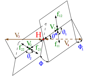
Figure 5: Illustrations of an $H$ boson production and decay in three topologies: (1) boson fusion and decay $V_{3}V_{4}\to H\to V_{1}V_{2}\to 4f$; (2) boson fusion with associated jets $q_{12}q_{22}\to q_{11}q_{21}(V_{1}V_{2}\to H\to V_{3}V_{4})$; and (3) associated production $q_{11}q_{12}\to V_{1}\to V_{2}(H\to V_{3}V_{4})$. Five angles fully characterize the orientation of the production or decay chain and are defined in suitable frames Gao:2010qx ; Anderson:2013afp .

In the $2\to 6$ process of associated $H$ boson production and its subsequent decay to a four-fermion final state, such as VBF, 13 kinematic observables are defined, which include angles and the invariant masses of intermediate states. There is also the overall boost of the six-body system, which depends on QCD effects. We decouple this boost from these considerations. Only a reduced set of observables is available when there are no associated particles in production or when the decay chain has less than four particles in the final state.

Kinematic distributions with anomalous couplings of the $H$ boson have been shown previously in Refs. Gao:2010qx ; Bolognesi:2012mm ; Anderson:2013afp for both decay and associated production. Here, we emphasize kinematics in associated production with two jets, shown in Fig. 6. There are distinct features depending on the $gg$, $\gamma\gamma$, $Z\gamma$, $ZZ$, and $WW$ fusion, which is reflected in the associated jet kinematics. Note that for the production processes we define $q_{i}^{2}$ for each vector boson, where $q_{i}^{2}<0$ for boson fusion and we therefore plot $\sqrt{-q_{i}^{2}}$. In this case, $\theta_{i}^{\rm assoc}$ angles, usually defined in the rest frame of the vector bosons, are calculated in the $H$ frame instead. We would like to stress that a consistent treatment of all contributions with $\gamma\gamma$, $Z\gamma$, $ZZ$, and $WW$ intermediate states in weak boson fusion is critical in a study of anomalous couplings.

While for the SM $H$ boson one could often neglect photon intermediate states when couplings to the $Z$ and $W$ bosons dominate, one generally cannot neglect them when comparing to other contributions generated by higher-dimension operators. In reference to the EFT operators discussed in Section II, the Higgs basis becomes the natural one to disentangle the $H\gamma\gamma$, $HZ\gamma$, $HZZ$, and $HWW$ operators from the experimentally observed kinematics of events. This is visible, for example, in the $q_{1,2}^{\rm VBF}$ distributions corresponding to the pseudoscalar operators, where the photon intermediate states lead to a much softer spectrum compared to $W$ and $Z$. The advantage of the Higgs basis for experimental analysis becomes especially evident when considering off-shell effects, because there is no off-shell enhancement with the intermediate $\gamma$ states. Once experimental results are obtained in the Higgs basis, the measurements can be translated to any other basis.

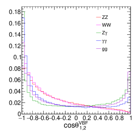
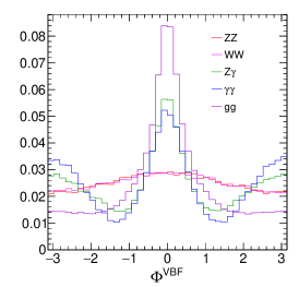
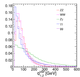
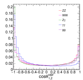
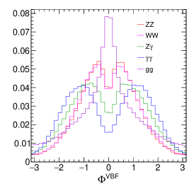
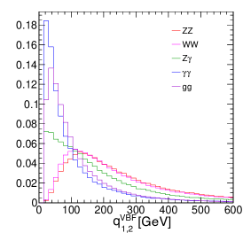
Figure 6: Distributions of observables in vector boson fusion jet associated production: $\{\theta_{1,2}^{\rm VBF},\Phi^{\rm VBF},\sqrt{-q_{1,2}^{2,\rm VBF}}\}$, comparing $gg$, $\gamma\gamma$, $Z\gamma$, $ZZ$, and $WW$ fusion for the SM couplings (top) and pseudoscalar couplings (bottom). A loose selection, $\Delta R_{JJ}>0.3$ and $p_{T}^{J}>15\,\text{GeV}$, is applied, consistently for all processes, to avoid divergences in processes with photons and gluons. All distributions are normalized to unit area.

With up to 13 observables ${\bf\Omega}$ sensitive to the Higgs boson anomalous couplings, it is a challenging task to perform an optimal analysis in a multidimensional space of observables, creating the likelihood function depending on more than a dozen parameters in Eq. (7). Full detector simulation and data control regions in LHC data analyses may limit the number of available events and, as a result, the level of detail in the likelihood. Therefore, it is important to develop methods that are close to optimal under the practical constraints of the available data and simulation. In the rest of this Section, we discuss some of the experimental applications of the tools developed in our framework, which target these tasks in the study of the $H$ boson kinematics.

Analysis of experimental observables typically requires the construction of a likelihood function, which is maximized with respect to parameters of interest. The complexity of the likelihood function grows quickly both with the number of observables and with the number of parameters, and the two typically increase simultaneously. Examples of such likelihood construction will be discussed in Section VI. Typically, the likelihood function will be parameterized with templates (histograms) of observables, using either simulated MC samples or control regions in the data. The challenge in this approach is to keep the number of bins of observables to a practical limit, typically several bins for several observables, due to statistical limitations in the available data and simulation. Similar practical limitations appear in the number of parameters of interest, which will be discussed later.

The information content in the kinematic observables is different, and one could pick some of the most informative kinematic observables of interest. The difficulty of this approach is illustrated in Fig. 6 where all five observables (note that $\theta_{1,2}$ and $q_{1,2}$ each represent two independent observables) provide important information and it is hard to pick a reduced set without substantial loss of information. Another approach is to create new observables optimal for the problem of interest, and in the next subsections we illustrate optimal observables based on both the matrix element and the machine learning techniques. Nonetheless, it is not possible to have a prior best set of observables universally good for all measurements and at the same time limited in the number of dimensions for practical reasons. We note that alternative methods may try to avoid creation of templates and parameterize the multi-dimensional likelihood function directly with certain approximations. We illustrated some of these methods in Refs. Gao:2010qx ; Anderson:2013afp and a broader review may be found in Ref. Brehmer:2019bvj . However, the complexity of those methods also provides practical limitations on their application. We present some of the practical approaches in Section VI.

One popular example of the reduced set of bins of observables adopted for the study of the $H$ boson kinematics is the so-called Simplified Template Cross Section approach (STXS) deFlorian:2016spz ; Berger:2019wnu . The main focus at this stage Berger:2019wnu is on the three dominant $H$ boson production processes, namely gluon fusion, VBF, and $VH$. These main production processes are subdivided into bins based on transverse momentum or mass of various objects, for example the $H$ boson and associated jets. At future stages, the available information may be subdivided further. This approach became a strong framework for collaborative work of both theorists and experimentalists, as information from all LHC experiments and theoretical calculations can be combined and shared in an efficient way. Nonetheless, as we illustrate below, this approach is still limited in its application for two important reasons. First, the STXS measurements are based on the analysis of SM-like kinematics. The measurement strategy may not be appropriate for interpretations appearing with new tensor structures or new virtual particles (such as $\gamma^{*}$ in place of $Z^{*}$) unless a full detector simulation of such effects is performed. Additionally, the binning of STXS may not be optimal for all the measurements of interest.

V.1 Matrix element technique

The matrix element likelihood approach (MELA) Gao:2010qx ; Bolognesi:2012mm ; Anderson:2013afp ; Gritsan:2016hjl was designed to extract all essential information from the complex kinematics of both production and decay of the $H$ boson  and retain it in the minimal set of observables. Two types of discriminants were defined for either the production or the decay process, and here we generalize it for any sequential process of both production and decay:

$${\cal{D}_{\rm alt}}({\bf\Omega})=\frac{{\cal P}_{\rm sig}({\bf\Omega})}{{\cal P}_{\rm sig}({\bf\Omega})+{\cal P}_{\rm alt}({\bf\Omega})}\,,$$ (44)

$${\cal{D}_{\rm int}}({\bf\Omega})=\frac{{\cal P}_{\rm int}({\bf\Omega})}{2\sqrt{{\cal P}_{\rm sig}({\bf\Omega})\times{\cal P}_{\rm alt}({\bf\Omega})}}\,,$$ (45)

where ${\cal P}_{\rm sig}$, ${\cal P}_{\rm alt}$, and ${\cal P}_{\rm int}$ represent the probability distribution for a signal model of interest, an alternative model to be rejected (either background, a different production process of the $H$ boson, or an alternative anomalous coupling of the $H$ boson), and the interference contribution, which may in general be positive or negative. The probabilities are obtained from the matrix elements squared, calculated by the MELA library described in Section IV, and do not generally need to be normalized. The denominator in Eq. (45) is chosen to reduce correlation between the discriminants, but this choice is equivalent to that of Ref. Anderson:2013afp . The above definition leads to the convenient arrangement $0\leq\cal{D}_{\rm alt}\leq$ 1 and $-1\leq\cal{D}_{\rm int}\leq$ 1.

These discriminants retain all multidimentional correlations essential for the measurements of interest. For a simple discrimination of two hypotheses, the Neyman-Pearson lemma Neyman:1933 guarantees that the ratio of probabilities ${\cal P}$ for the two hypotheses provides optimal discrimination power. However, for a continuous set of hypotheses with an arbitrary quantum-mechanical mixture several discriminants are required for an optimal measurement of their relative contributions. There are three interference discriminants when anomalous couplings appear both in production and in decay. Let us conside only real $g_{1}$ and $g_{4}$ couplings in Eq. (1), which appear once in production and once in decay, as shown in Eq. (32). The total amplitude squared would have five terms proportional to $(g_{4}/g_{1})^{m}$ with $m=0,1,2,3,4$:

$$\mathcal{P}^{\mathrm{}}\left({\bf\Omega};g_{1},g_{4}\right)\\ \propto\sum_{m=0}^{4}(g_{4}/g_{1})^{m}\times\mathcal{P}^{\mathrm{}}_{m}\left({\bf\Omega}\right)\,,$$ (46)

where we absorb $g_{1}^{4}$ and the width into the overall normalization. Equation (44) corresponds to the ratio of the $m=4$ and $m=0$ terms. Three other ratios give rise to interference discriminants. The four discriminants may be re-arranged into two discriminants of the form in Eq. (44) and two of the form in Eq. (45), in each case one observable defined purely for the production process and the other for the decay process. One could apply the Neyman-Pearson lemma to each pair of points in the parameter space of $(g_{1},g_{4})$, but this would require a continuous, and therefore infinite, set of probability ratios. However, equivalent information is contained in a linear combination of only four probability ratios, which can be treated as four independent observables. Above the $2m_{V}$ threshold, there are also interference discriminants appearing due to interference between the off-shell tail of the signal process and the background. A subset of equivalent optimal observables was also introduced independently in earlier work on different topics Atwood:1991ka ; Davier:1992nw ; Diehl:1993br .

The number of discriminants in Eqs. (44, 45) is still limited if we consider just one anomalous coupling. Nonetheless, this number grows quickly as we consider multiple anomalous couplings, especially the number of interference discriminants. A subset of these discriminants may contain most of the information, depending on the situation. For the near-term LHC measurements, the $\cal{D}_{\rm alt}$ using full production and decay information and $\cal{D}_{\rm int}$ using production information from correlation of associated particles provide the most optimal information. In the very long term, the lowest powers of $m$ may provide most of the discriminating power when testing data for tiny anomalous contributions, because effects may be most visible in interference. Therefore, the MELA approach still allows us to select a limited set of the most optimal discriminants, as we illustrate with the practical applications below.

Detector resolution effects may come into play in experimental analyses and affect the calculations of the probabilities in Eqs. (44, 45). These can be parameterized with transfer functions. However, in most practical applications, the “raw” matrix element probabilities can be used, and the resulting performance degradation is small when the distributions of the angular and mass observables are broad compared to the resolution. One notable exception is the invariant mass of relatively narrow resonances, such as the $H$ boson mass in $H\to ZZ\to 4\ell$ or the $V$ boson mass in associated production $VH$. In such a case, the signal and background probabilities ${\cal P}_{\rm sig}$ and ${\cal P}_{\rm bkg}$ can incorporate the empirical invariant mass parameterization giving rise to the ${D_{\rm bkg}}$ discriminant for optimal background rejection. We find such an approach computationally effective without any visible loss of performance. Nonetheless, below we also introduce machine learning to enhance the matrix element technique. This approach incorporates matrix element knowledge combined with the parton shower and detector effects.

V.2 Application of the matrix element technique to the boson fusion processes

Let us illustrate the power of the matrix element technique in application to both weak boson fusion (VBF in the following) and strong boson fusion (ggH in the following), where at higher orders in QCD the ggH process may include $gg,qg,$ and $qq$ initial states. This illustration is similar to our earlier study in Ref. Anderson:2013afp , but we would like to expand this illustration in several directions. The boson fusion process is particularly important in the off-shell region, which is a new feature of this work. However, most kinematic considerations apply equally to both the on-shell and off-shell regions. In the weak boson fusion, for illustration purposes we consider equal strength of $WW$ and $ZZ$ fusion, with $g_{1}^{ZZ}=g_{1}^{WW}$ and $g_{4}^{ZZ}=g_{4}^{WW}$ in Eq. (1) and vary the relative contribution of the CP-even and CP-odd amplitudes, with the $f_{g4}^{\rm VBF}$ parameter representing their relative cross section fraction. The relative strength of $WW$ and $ZZ$ fusion is fixed in this study because the two processes are essentially indistinguishable in their observed kinematics, as shown in Fig. 6. In strong boson fusion, the parameter $f_{g4}^{ggH}$ represents a similar relative cross section fraction of the pseudoscalar coupling component.

Figure 7 shows the $\mathcal{D}_{0-}$ and ${\cal D}_{\rm CP}$ discriminants, calculated according to Eqs. (44) and (45), for the VBF process, to distinguish between the SM hypothesis $g_{1}^{ZZ}=g_{1}^{WW}=2$, the alternative hypothesis $g_{4}^{ZZ}=g_{4}^{WW}\neq 0$, and the interference between these two contributions. Figure 8 shows the same type of discriminants defined and shown for the ggH process, enhanced with the events in the VBF-like topology using the requirement $m_{JJ}>300$ GeV for illustration. In both cases, information from the $H$ boson and the two associated jets, as illustrated in Fig. 5, is used in the discriminant calculation. The $m_{JJ}$ requirement is based on the following observation. Among the initial states in the ggH process, we could have $gg,qg,$ and $qq$ parton pairs. The events with the $qq$ initial state carry most of the information for CP measurements and have the topology most similar to the VBF process, which is also known to have a large di-jet invariant mass. In Section VI, we will use this feature when developing the analysis techniques, but with the matrix-element technique applied to isolate the VBF-like topology. In both the VBF and ggH cases, the azimuthal angle difference between the two jets $\Delta\Phi_{JJ}$ is also shown for comparison Plehn:2001nj . It is similar to the $\Phi^{\rm VBF}$ angle defined in Fig. 5 and shown in Fig. 6, but differs somewhat because it is calculated in a different frame.

The $\Delta\Phi_{JJ}$ angle is defined as follows. The direction of the two jets is represented by the vectors $\vec{j}_{1,2}$ in the laboratory frame, and $\vec{j}_{T1,2}$ are the transverse components in the $xy$ plane. If we label $j_{1}$ as the jet going in the $-z$ direction (or less forward) and $j_{2}$ as the jet going in the $+z$ direction (or more forward), then $\Delta\Phi_{JJ}$ is the azimuthal angle difference between the first and the second jets, or $\phi_{1}-\phi_{2}$. In vector notation,

$$\Delta\Phi_{JJ}=\frac{(\hat{j}_{T1}\times\hat{j}_{T2})\cdot\hat{z}}{|(\hat{j}_{T1}\times\hat{j}_{T2})\cdot\hat{z}|}\cdot\frac{(\vec{j}_{1}-\vec{j}_{2})\cdot\hat{z}}{|(\vec{j}_{1}-\vec{j}_{2})\cdot\hat{z}|}\cdot\cos^{-1}\left(\hat{j}_{T1}\cdot\hat{j}_{T2}\right)\,,$$ (47)

where the angle between $\vec{j}_{T1}$ and $\vec{j}_{T2}$ defines $\Delta\Phi_{JJ}$ and the two ratios provide the sign convention. This definition is invariant under the exchange of the two jets and the choice of the positive $z$ axis direction.

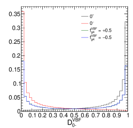
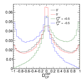
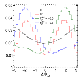
Figure 7: Two discriminants defined in Eq. (44) (left) and Eq. (45) (middle) for the measurement of the CP-sensitive parameter $f_{g4}^{\rm VBF}$ in VBF production. Also shown is the $\Delta\Phi_{JJ}$ observable (right). The values of $f_{g4}^{\rm VBF}=\pm 0.5$ correspond to 50% mixtures of the CP-even and CP-odd contributions.

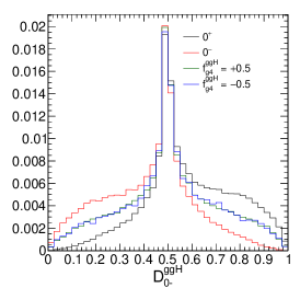
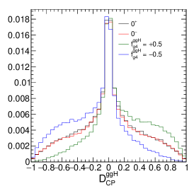
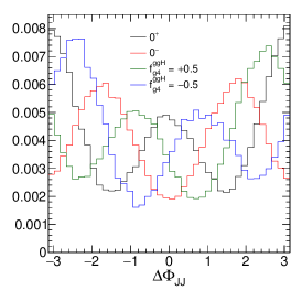
Figure 8: Two discriminants defined in Eq. (44) (left) and Eq. (45) (middle) for the measurement of the CP-sensitive parameter $f_{g4}^{\rm ggH}$ in ggH production. Also shown is the $\Delta\Phi_{JJ}$ observable (right). The values of $f_{g4}^{\rm ggH}=\pm 0.5$ correspond to 50% mixtures of the CP-even and CP-odd contributions. A requirement $m_{JJ}>300$ GeV is applied to enhance the VBF-like topology of events.

The information content of the observables can be illustrated with the Receiver Operating Characteristic (ROC) curve, which is a graphical plot that illustrates the diagnostic ability of a binary classifier system as its discrimination threshold is varied. Figure 9 (left) shows the ROC curves illustrating discrimination between scalar and pseudoscalar models in the VBF process using the ${\cal D}_{0-}$ and $\Delta\Phi_{JJ}$ observables. The optimal observable ${\cal D}_{0-}$, which incorporates all kinematic and dynamic information, has the clear advantage. Figure 9 (right) shows the same comparison in the ggH process. The gain in using the optimal observable in the ggH process is not as large as in VBF because of the smaller differences in dynamics of the scalar and pseudoscalar models, as both are generated by higher-dimension operators with the same powers of $q_{i}^{2}$ in Eq. (1). While the ${\cal D}_{0-}$ observable incorporates all kinematic and dynamic information, the truly CP-sensitive observable ${\cal D}_{\rm CP}$ does not rely on dynamics. It provides optimal separation between the models with maximal mixing of the CP-even and CP-odd contributions and opposite phases. We illustrate this in Fig. 9 (middle) with a ROC curve for discrimination between the $f_{g4}=\pm 0.5$ models in the VBF process.

V.3 Matrix element technique with machine learning

The discriminants calculated with the matrix elements directly, as discussed in Section V.1, are powerful tools in the analysis of experimental data. Most importantly, they provide scientific insight into the problem under study. Nonetheless, there could be practical considerations limiting their application in certain cases. For example, events with partial reconstruction would require integration over unobserved degrees of freedom. Substantial detector effects or incorrect particle assignment in reconstructed events may lead to poor experimental resolution and would require modeling with transfer functions. All of these effects can be taken into account, but may make calculations inefficient or impractical. Here we provide a practical prescription for overcoming these complications with the help of machine learning, while still retaining the functionality of the optimal matrix-element approach. We achieve this by constructing the training samples and the observables used according to the matrix-element approach.

Machine learning is a popular approach to data analysis, especially with the growing computational power of computers. The problem of differentiating between two models, as in Eq. (44), becomes a trivial task with supervised learning, where two samples of events with the signal and alternative models are provided as input for training. One key aspect where the matrix element approach provides the insight is the set of input observables ${\bf\Omega}$. As long as the complete set of observables, sufficient for the matrix element calculations, is provided to the machine learning algorithm, the outcome of proper training is guaranteed to be a discriminant optimal for this task, equivalent to that in Eq. (44). We illustrate this with such a discriminant ${\cal D}_{0-}^{\rm ML}$ in Fig. 9 (left) in application to the VBF process, using the Boosted Decision Tree implementation from Ref. Hocker:2007ht .

Application of the machine learning approach to the discriminant in Eq. (45) is less obvious, because it requires knowledge of quantum mechanics to isolate the interference component. Nonetheless, we provide a prescription for obtaining such a discriminant. A discriminant trained to differentiate the models with maximal quantum-mechanical mixing of the signal and alternative contributions with opposite phases becomes a machine-learning equivalent to that in Eq. (45), following the discussion in Section V.2. The complete kinematic information ${\bf\Omega}$ of the event should be provided to training. We illustrate this approach with such a discriminant ${\cal D}_{\rm CP}^{\rm ML}$ in Fig. 9 (middle) in application to the VBF process. There is a small degradation in performance of the ${\cal D}_{\rm CP}^{\rm ML}$ discriminant with respect to the matrix element calculation, but this is attributed to the more challenging task of training in this case and should be recovered in the limit of perfect training.

To summarize, the matrix element technique, expressed in Eqs. (44) and (45), can be expanded with the help of machine learning with two important ingredients: (1) the complete set of matrix-element input observables ${\bf\Omega}$, or equivalent, has to be used, and (2) the machine learning process should be based on the carefully prepared samples according to the models discussed above. The machine learning approach is still based on the matrix element calculations, as the training samples are generated based on the same matrix elements as the discriminants in Eqs. (44) and (45).

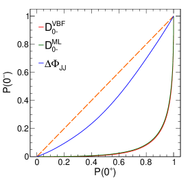
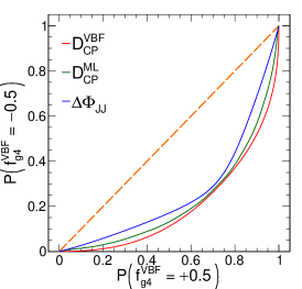
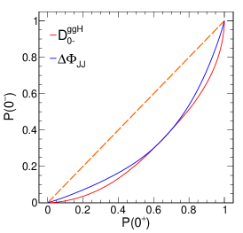
Figure 9: Left: a ROC curve showing the separation power between the scalar (SM-like $0^{+}$) and pseudoscalar ($0^{-}$) models in the VBF process using the ${\cal D}_{0-}$ and $\Delta\Phi_{JJ}$ observables. The diagonal dashed line shows the hypothetical no-separation scenario. The points represent the efficiency of selecting each model as the threshold of selection is varied. Right: same as the left plot, but for the ggH process, with a requirement $m_{JJ}>300$ GeV applied to enhance the VBF-like topology of events. Middle: a ROC curve showing the separation power between the $f_{g4}^{\rm VBF}=+0.5$ and $f_{g4}^{\rm VBF}=-0.5$ models in the VBF process using the ${\cal D}_{\rm CP}$ and $\Delta\Phi_{JJ}$ observables. Also shown on the left and middle plots are the ROC curves representing performance of the optimal observables obtained with machine learning techniques.

VI Application to on-shell H(125) boson production

We start by investigating the on-shell production and decay of the $H$ boson with its coupling to either weak or strong vector bosons in the VBF and ggH processes. There has already been extensive study of the $HVV$ couplings, and the current challenge is in the measurement of multiple possible anomalous contributions. On the other hand, there have been limited studies of the anomalous $Hgg$ couplings, due to lower statistical precision at this time. The latter could be interpreted as both an effective coupling to gluons, or as a coupling to quarks in the gluon fusion loop. Prospects of both $HVV$ and $Hgg$ studies with either 3000 $fb^{-1}$ (HL-LHC) or 300 $fb^{-1}$ (full LHC) are presented below. Let us first discuss some general features in analysis of LHC data.

For the $HVV$ studies, we will use the example of the $H\to VV\to 4\ell$ decay and VBF, $VH$, or ggH production. Equation (1) defines several anomalous couplings, which we generically denote as $g_{i}^{VV}$. All of these processes include the interference of several $VV$ intermediate states, such as ${VV}=ZZ,Z\gamma,\gamma\gamma,WW$. In the analysis of the data (MC simulation in our case), a likelihood fit is performed Verkerke:2003ir ; Brun:1997pa . The probability density function for a given signal process, before proper normalization, is defined for the two possible numbers of couplings $N$ in the product:

$$N=4:~{}~{}~{} \mathcal{P}\left({\bf x};\vec{f}\,\right)\propto\sum_{\begin{subarray}{c}k,l,m,n=1\\ k\leq l\leq m\leq n\end{subarray}}^{K}\mathcal{P}_{klmn}\left({\bf x}\right)\sqrt{|f_{gk}\cdot f_{gl}\cdot f_{gm}\cdot f_{gn}|}~{}\mathrm{sign}(f_{gk}\cdot f_{gl}\cdot f_{gm}\cdot f_{gn})\,,$$ (48)

$$N=2:~{}~{}~{} \mathcal{P}\left({\bf x};\vec{f}\,\right)\propto\sum_{\begin{subarray}{c}k,l=1\\ k\leq l\end{subarray}}^{K}\mathcal{P}_{kl}\left({\bf x}\right)\sqrt{|f_{gk}\cdot f_{gl}|}~{}\mathrm{sign}(f_{gk}\cdot f_{gl})\,,$$ (49)

where ${\bf x}$ are the observables, but not necessarily the complete set ${\bf\Omega}$, and $f_{gn}$ are $K$ terms corresponding to the cross-section fractions of the couplings, defined in Eq. (42). Equations (48) and (49) are obtained from Eq. (32) and using Eq. (43), where the width and $f_{g1}$ are absorbed into the overall normalization. In the case of the electroweak process, the $HVV$ coupling appears on both the production and the decay sides. As a result, the amplitude squared has a product of $N=4$ couplings. In the gluon fusion production, on the other hand, the electroweak $HVV$ couplings appear only in decay, and therefore $N=2$. Similarly, if one considers the $Hgg$ coupling on production, $N=2$.

There are $(N+K-1)!/(N!(K-1)!)$ terms in either Eq. (48) or Eq. (49). As we explain in Section VI.1, we consider $K=5$ in our analysis of four anomalous $HVV$ couplings. Therefore, in the case of electroweak production ($N=4$, $K=5$), we have to deal with 70 terms. If we were to consider $K=13$ independent couplings in Eq. (1), we would formally have to deal with 1820 terms describing production and decay (the actual number would be somewhat smaller because not all terms contribute to a given decay mode). While such analysis of 1820 terms is in principle feasible, at the current stage it is not practical. In the case of gluon fusion, there are 15 terms for $HVV$ couplings ($N=2$, $K=5$) and 3 terms for $Hgg$ couplings ($N=2$, $K=2$). If both sets of anomalous couplings are considered simultaneously, the total number of terms is the product of these, that is 45.

In the simplified analysis of LHC data, using simulation of $pp$ collisions at 13 TeV, we adopt the following approach. We take the analysis of the $H\to VV\to 4\ell$ channel as the most interesting for illustration, because both production and decay information can be used. All production modes of the $H$ boson are included in this study and are generated with the JHU generator as discussed in Section IV. The JHU generator framework is also used to generate gluon fusion and electroweak background production of the $VV\to 4\ell$ final states. The dominant $q\bar{q}\to VV\to 4\ell$ background process is generated with POWHEG powhegvv and scaled to cover for other possible background contributions not modeled otherwise CMS-HIG-19-001 . All events are passed through Pythia 8 Sjostrand:2014zea for parton shower simulation. The detector effects are modeled with ad-hoc acceptance selection, and the lepton and hadronic jet momenta are smeared to achieve realistic resolution effects. Going beyond the $H\to 4\ell$ channel, inclusion of the $H\to\gamma\gamma$, $H\to\tau\tau$, and $H\to bb$ channels might increase the dataset by about an order of magnitude, but only for analysis of the production information. In addition, analysis of the $H\to WW\to 2\ell 2\nu$ decay may bring some information on the decay side, but not exceeding that from the $H\to 4\ell$ case. While we focus on the $H\to 4\ell$ channel, we comment on improvements which will be achieved with a combination of the above channels.

VI.1 HVV anomalous couplings

In order to illustrate the power of the matrix element techniques and the analysis tools discussed above, let us consider the $HVV$ coupling of the $H$ boson to two weak vector bosons using the $H\to 4\ell$ decay, with vector boson fusion, associated production with the vector bosons $W$ and $Z$, or inclusive production, and using both on-shell and off-shell production. Some of these techniques have already been applied in analyses of LHC data Sirunyan:2017tqd ; Sirunyan:2019twz ; Sirunyan:2019nbs . However, the rich kinematics in production and decay of the $H$ boson represents particular challenges in analysis.

There are 13 independent $HVV$ anomalous couplings in Eq. (1). An optimal simultaneous measurement of all these couplings, or even a sizable subset, represents a practical challenge in data analysis and, as far as we know, has not been attempted experimentally yet. Here we stress that an optimal measurement means that the precision of any given parameter measurement is not degraded when comparing a multi-parameter approach with all other couplings constrained and an optimal single-parameter measurement discussed below. Several approaches have been adopted. In one approach, a small number of couplings, typically two or at most three, is considered. One of these is the SM-like coupling and the other could be parameterized with the cross-section fraction $f_{gi}$ defined above. While this approach is optimal for each parameter measurement, the problem with this approach is that correlations between measurements of different anomalous couplings are not considered.

Another recently adopted approach is the STXS measurement, where cross sections of several $H$ boson production processes are measured in several bins based on kinematics of the event. While this approach is attractive due to its applicability to a number of various use cases, the problems with this approach are that observables are not necessarily optimal for any given measurement, and that the kinematics of events are assumed to follow the SM when measuring the cross section in each bin. For a correct measurement, a full detector simulation of each coupling scenario is needed, because the kinematics of associated particles and decay products would affect the measurement in each bin. The STXS approach based on SM-only kinematics does not include these effects. The latter effect is especially important because neglecting it may lead to biases in the measurements. In the following, we illustrate the strengths and weaknesses of each approach, and propose a practical method based on the matrix element approach.

First, we would like to note that it is difficult to perform an unambiguous measurement of all 13 independent $HVV$ anomalous couplings in Eq. (1) in a given process. For example, while all these couplings contribute to the VBF production, kinematics of $WW$ and $ZZ$ fusion are essentially identical, as shown in Fig. 6. The measurement becomes feasible when the $WW$ and $ZZ$ couplings are related. We adopt two examples of this relationship. In one case, we simply set $g_{i}^{WW}=g_{i}^{ZZ}$, which could be interpreted as relationships in Eqs. (17–20) under the $c_{w}=1$ condition. Such results could be re-interpreted for a different relationship of the couplings. In the second case, we adopt the relationships in Eqs. (17–21) without any conditions. With such a simplification, we are still left with nine parameters in the first case and eight parameters in the second case. To simplify the analysis further, we reduce the number of free parameters by setting $g_{2}^{\gamma\gamma}=g_{4}^{\gamma\gamma}=g_{2}^{Z\gamma}=g_{4}^{Z\gamma}=0$. While we do expect to observe non-zero values of $g_{2}^{\gamma\gamma}$ and $g_{2}^{Z\gamma}$ even in the SM, constraints on all four couplings are possible from decays $H\to\gamma\gamma$ and $Z\gamma$ with on-shell photons. We leave the exercise to include all couplings in an optimal analysis to future studies. In addition, we keep the $g_{2}^{gg}$ and $g_{4}^{gg}$ couplings as two free parameters as well. While the dedicated studies of these couplings are presented in Section VI.2, kinematics of the ggH process may affect measurements in the VBF process.

As a reference, we take the STXS stage-1.1 binning as applied by the CMS experiment CMS-HIG-19-001 ; deFlorian:2016spz . In this approach, seven event categories are defined, which are optimal for separating the VBF topology with two associated jets; two $VH$ categories, with leptonic and hadronic decay of the $V$, respectively; the VBF topology with one associated jet; two $t\bar{t}H$ categories, with leptonic and fully hadronic top decay, respectively; and the untagged category, which includes the rest of the events. We call it stage-0 categorization. Each category of events is further split into sub-categories to match the requirements on the transverse momenta and invariant masses, as defined in the STXS stage-1.1 binning. In total, there are 22 categories defined CMS-HIG-19-001 . While the above STXS stage-1.1 categorization provides fine binning for capturing some kinematic features in production of the $H$ boson, it does not keep any information from decay, it has no information sensitive to $CP$ violation, and more generally, it is not guaranteed to be optimal for measuring any of the parameters of our interest.

Since we target the optimal analysis of four anomalous couplings expressed through $f_{g4}$, $f_{g2}$, $f_{\Lambda 1}$, and $f_{\Lambda 1}^{Z\gamma}$, we build the analysis in the following way. Instead of STXS stage-1.1 binning, we start from the seven categories defined in stage-0 for isolating different event topologies. Since in this analysis we do not target fermion couplings, the two $t\bar{t}H$ categories are merged with the untagged category. There are four discriminants relevant for this analysis, as defined by Eq. (44): ${\cal D}_{g4}$, ${\cal D}_{g2}$, ${\cal D}_{\Lambda 1}$, and ${\cal D}_{\Lambda 1}^{Z\gamma}$. In addition, two interference discriminants, ${\cal D}_{\rm CP}$ and ${\cal D}_{\rm int}$, are defined by Eq. (45) for the $g_{4}$ and $g_{2}$ couplings, respectively. The two other interference discriminants are found to provide little additional information due to large correlations with the discriminants defined in Eq. (44). The full available information is used in calculating the discriminants in the following way. In the untagged category, the $H\to VV\to 4\ell$ information is used. In addition, the transverse momentum of the $H$ boson is included, because it is sensitive to production. In both the VBF and $VH$ topologies with two associated jets, both production and decay information are used, except for the two interference discriminants, where production information is chosen because it dominates. In the leptonic $VH$ category and the VBF topology with one associated jet, where information is in general missing, the transverse momentum of the $H$ boson is used, with finer binning than in the untagged category. In the end, for each event in a category $j$ a set of observables ${\bf x}$ is defined.

To parameterize the 70 terms in Eq. (48) or the 15 terms in Eq. (49), we rely on samples generated with JHUGen. However, it is not necessary to generate 70 or 15 separate samples. Instead, we generate a few samples that adequately cover the phase space and re-weight those samples using the MELA package to parameterize the other terms. To populate the probability distributions, we use a simulation of unweighted events with detector modeling, and small statistical fluctuations are inevitable. A critical step in the process is to ensure that even with these statistical fluctuations, the probability density function $\mathcal{P}$, defined in Eqs. (48) and (49), remains positive for all possible values of $\vec{f}$. We detect negative probability by minimizing $\mathcal{P}$, which is a polynomial in $\sqrt{|f_{gi}|}\cdot\mathrm{sign}(f_{gi})$. In the case of Eq. (48), where the polynomial is quartic, we use the Hom4PS program HomotopyContinuation ; Hom4PS1 ; Hom4PS2 to accomplish this minimization. If negative probability is possible, we modify $\mathcal{P}_{klmn}$ or $\mathcal{P}_{kl}$ using the cutting planes algorithm cuttingplanes , using the Gurobi program gurobi in each iteration of the procedure, until $\mathcal{P}$ is always positive. We find that only small modifications to $\mathcal{P}_{klmn}$ or $\mathcal{P}_{kl}$ are needed.

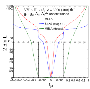
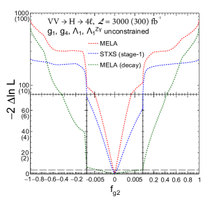
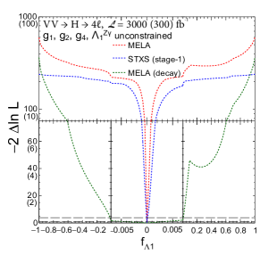
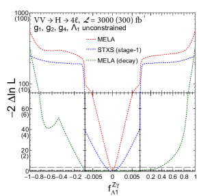
Figure 10: Expected constraints from a simultaneous fit of $f_{g4}$, $f_{g2}$, $f_{\Lambda 1}$, and $f_{\Lambda 1}^{Z\gamma}$ using associated production and $H\to 4\ell$ decay with 3000 (300) fb^-1 data. Three analysis scenarios are shown: using MELA observables with production and decay (or decay only) information, and using STXS binning. The dashed horizontal lines show the 68 and 95% CL regions.

In Fig. 10 we show the expected constraints on the four parameters of interest $f_{g4}$, $f_{g2}$, $f_{\Lambda 1}$, and $f_{\Lambda 1}^{Z\gamma}$, using both associated production and $H\to 4\ell$ decay with 3000 fb^-1 (or 300 fb^-1) of data at a single LHC experiment. The constraints on each parameter are shown with the other parameters describing the $HVV$ and $Hgg$ couplings profiled, including $f_{\rm CP}^{\rm gg}$ and the signal strength parameters $\mu^{V}$ and $\mu^{f}$. The $\mu^{V}$ and $\mu^{f}$ parameters correspond to production strength of electroweak and other processes, respectively. Therefore, there are a total of seven free parameters describing $HVV$ and $Hgg$ couplings. The MC scenario has been generated with the SM expectation. The production information dominates in all constraints. However, as discussed in Section II.5, this is due to unbounded growth of anomalous couplings with $q^{2}$. Since this behavior cannot continue forever, it is still interesting to look at the decay-only constraints, which do not rely on the $q^{2}$-dependent growth of the amplitude. Therefore, in Fig. 10 both kinds of constraints are shown for illustration of the two limiting cases. We point out that form factor scaling, such as introduced in Eq. (30), can be used for continuous study of this effect.

In addition, a comparison is made to the approach where instead of the optimal discriminants, the STXS stage-1.1 bins are used as observables, while using full simulation of all processes otherwise. There is a significant difference in expected precision. The most striking effect is the lack of constraints from decay information, but there is a loss in precision using production information in STXS as well. It is interesting to point that there is still weak decay-related information in the categories used in the STXS approach, because interference between identical leptons produces different rates of $2e2\mu$ events compared to $4e$ and $4\mu$, depending on the couplings.

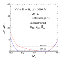
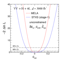
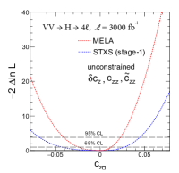
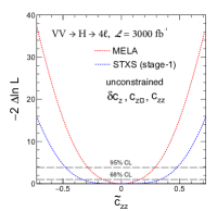
Figure 11: Expected constraints from a simultaneous fit of (from left to right) $\delta c_{z}$, $c_{zz}$, $c_{z\Box}$, and $\tilde{c}_{zz}$ using associated production and $H\to 4\ell$ decay with 3000 fb^-1 data. The EFT coupling constraints are the result of re-interpretation from the signal strength and $f_{gi}$ measurements discussed in text. The constraints on each parameter are shown with the other parameters describing the $HVV$ and $Hgg$ couplings profiled. Two analysis scenarios are shown: using MELA observables and using STXS binning. The dashed horizontal lines show the 68 and 95% CL regions.

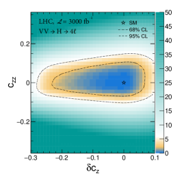
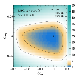
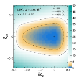
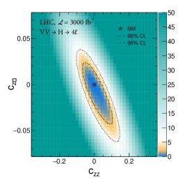
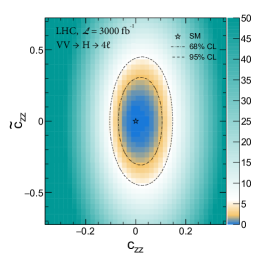
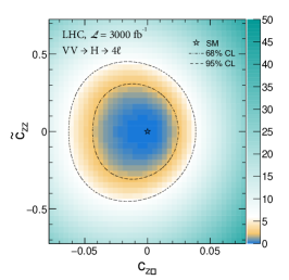
Figure 12: Expected two-dimensional constraints from a simultaneous fit of $\delta c_{z}$, $c_{zz}$, $c_{z\Box}$, and $\tilde{c}_{zz}$ as shown in Fig. 11 for the MELA observables. The constraints on each parameter are shown with the other parameters describing the $HVV$ and $Hgg$ couplings profiled. Top-left: $(\delta c_{z},c_{zz})$; top-middle: $(\delta c_{z},c_{z\Box})$; top-right: $(\delta c_{z},\tilde{c}_{zz})$; bottom-left: $(c_{zz},c_{z\Box})$; bottom-middle: $(c_{zz},\tilde{c}_{zz})$; bottom-right: $(c_{z\Box},\tilde{c}_{zz})$.

Since $f_{gi}$ measurements involve ratios of couplings, most systematic uncertainties that would otherwise affect the cross section measurements cancel in the ratio. Therefore, the $f_{gi}$ measurements are still expected to be statistics limited with 3000 fb^-1 of data. For this reason, the expected results can be easily reinterpreted for another scenario of integrated luminosity, as for example the expectation with 300 fb^-1 shown in parentheses. However, when the $f_{gi}$ measurements are re-interpreted in terms of couplings (as we illustrate below), both the signal strength and the $f_{gi}$ results need to be combined. This leads to sizable systematic uncertainties affecting the couplings. In the following, we assign 5% theoretical and 5% experimental uncertainties on the measurements of the signal strength, which is the ratio of the measured and expected cross sections.

We also perform a fit with three cross-section fraction parameters $f_{g4}$, $f_{g2}$, and $f_{\Lambda 1}$ with the EFT relationship among couplings following Eqs. (17–21). The conclusions of this study are similar to those presented above. We re-interpret these results as constraints on the $\delta c_{z}$, $c_{zz}$, $c_{z\Box}$, and $\tilde{c}_{zz}$ couplings, defined in the EFT parameterization in the Higgs basis. This fit requires reinterpreting the process cross section and the three fractions in terms of couplings, and one has to take dependence of the width on the couplings into account, following Eq. (32). We assume that $\Gamma_{\rm other}=0$ and express the width using Eq. (34). The values of $\kappa_{f}=\kappa_{t}=\kappa_{b}=\kappa_{\tau}=\kappa_{\mu}$ and $\tilde{\kappa}_{f}=\tilde{\kappa}_{t}=\tilde{\kappa}_{b}=\tilde{\kappa}_{\tau}=\tilde{\kappa}_{\mu}$ are left unconstrained independently for the CP-even and CP-odd fermion couplings. The resulting one-dimensional constraints are shown in Fig. 11 and two-dimensional contours with the other parameters profiled are shown in Fig. 12. In Fig. 11 it is evident again that analysis based on the optimal discriminants provides the best constraints on the couplings of interest.

VI.2 Hgg anomalous couplings

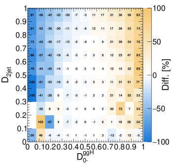
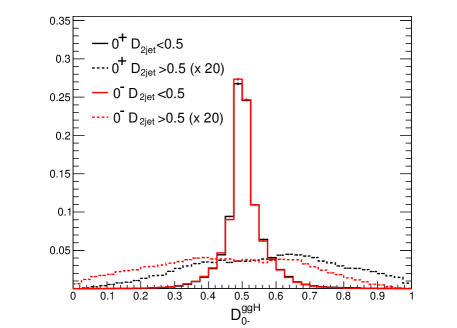
Figure 13: Left: The 2D distribution of the difference between the scalar and pseudoscalar populations of events for the ${\cal D}_{2\rm jet}$ and ${\cal D}_{0-}^{\rm ggH}$ discriminants, both self-normalized to 1, respectively. Right: ${\cal D}_{0-}^{\rm ggH}$ discriminant distributions of the scalar and pseudoscalar population events with the requirement on the ${\cal D}_{2\rm jet}$ discriminant below or above 0.5.

The gluon fusion process in association with two jets allows analysis of kinematic distributions for the measurement of potential anomalous contributions to the gluon fusion loop. Resolving the loop effects is a separate task, which we do not attempt to perform in this work. However, we point out that unless the particles in the loop are light, their mass does not significantly affect the kinematics of the $H$ boson and associated jets. The main effect is on the $H$ boson’s transverse momentum deFlorian:2016spz , where heavy particles in the loop may enhance the tail of the distribution at $p_{T}>200$ GeV, but will not significantly affect the bulk of the distribution relevant for our study, at $p_{T}<200$ GeV. Our analysis of the CP properties of this interaction depends primarily on the angular kinematics of the associated jets and $H$ boson, as discussed in Section V.2. Therefore, in the rest of this work we treat the gluon fusion process without resolving the loop contribution, allowing for any particles to contribute, either from SM or beyond. The only observable difference in this analysis is between the CP-even and CP-odd couplings, which can be parameterized as the overall strength of the $H$ boson’s coupling to gluons and the fraction of the CP-odd contribution $f_{\rm CP}^{\rm gg}$ defined in Eq. (42).

The analysis strategy follows the approach discussed in application to the $HVV$ measurements in the previous section, with the difference being the two-jet category optimized for the measurement of the gluon fusion process. In addition to a discriminant optimal for signal over background separation, the events are described by three observables. The ${\cal D}_{2\rm jet}$ observables follows Eq. (44), with the VBF and gluon fusion matrix elements used to isolate the VBF topology. The ${\cal D}_{0-}^{\rm ggH}$ and ${\cal D}_{\rm CP}^{\rm ggH}$ observables follow Eq. (44) and Eq. (45) for separating the SM-like coupling and CP-odd coupling, but with one modification to the process definition. Only the quark-initiated process defines the matrix element in these two formulas, because only such a VBF-like topology of the gluon fusion process carries relevant CP information. This is illustrated in Fig. 13, where the left plot shows that the ${\cal D}_{0-}^{\rm ggH}$ discriminant starts to separate the two couplings at higher values of ${\cal D}_{2\rm jet}$, which correspond to more VBF-like topology. The right plot shows that only at higher values of ${\cal D}_{2\rm jet}$ can one observe the separation. Only a small fraction of the total gluon fusion events end up in that region. This illustrates the challenge of the CP analysis in the gluon fusion process. The ${\cal D}_{\rm CP}^{\rm ggH}$ leads to forward-backward asymmetry in the distribution of events in the case of CP violation, when both CP-odd and CP-even amplitudes contribute.

A projection of $f_{\rm CP}^{\rm gg}$ sensitivity with 3000 and 300 fb^-1 at an LHC experiment is performed. The overall normalization of the gluon fusion production rate in the VBF-like topology is provided by the untagged events and events with two associated jets in a non-VBF topology. The electroweak VBF process is a background to the $f_{\rm CP}^{\rm gg}$ measurement in this case, but its kinematics are still distinct enough to keep it separated in the fit on the statistical basis. Keeping its CP properties unconstrained has little effect on the CP analysis in the gluon fusion process. We use the $H\to 4\ell$ analysis to illustrate the sensitivity, but scale the expected constraints with an effective luminosity ratio to account for the relative sensitivity of the $H\to\gamma\gamma$ and $\tau\tau$ channels based on the typical sensitivity in the VBF topology Sirunyan:2017tqd ; Sirunyan:2019nbs ; Sirunyan:2018koj ; Aad:2019mbh . The expected constraints are shown in Fig. 14. With 3000 (300) fb^-1, one can separate CP-even and CP-odd $Hgg$ couplings with a confidence level of about 9 (3) $\sigma$.

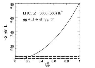
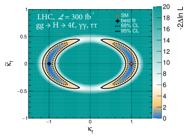
Figure 14: Expected constraints on $f_{\rm CP}^{\rm gg}$ with 3000 (300) fb^-1 (left) and $\kappa_{f}$ and $\tilde{\kappa}_{f}$ couplings in the gluon fusion loop with 300 fb^-1 (right), using the $H\to 4\ell,\gamma\gamma,$ and $\tau\tau$ decays. The dashed horizontal lines (left) and contours (right) show the 68 and 95% CL regions.

We re-interpret these expected constraints on $f_{\rm CP}^{\rm gg}$ and the cross section as constraints on the $\kappa_{f}=\kappa_{t}=\kappa_{b}$ and $\tilde{\kappa}_{f}=\tilde{\kappa}_{t}=\tilde{\kappa}_{b}$ couplings in the gluon fusion loop, assuming that only the SM top and bottom quarks dominate the loop. There are additional considerations when re-interpreting the signal strength and $f_{\rm CP}^{\rm gg}$ in terms of couplings following Eq. (32). As in the $HVV$ measurements in Section VI.1, we assume $\Gamma_{\rm other}=0$ and express the width $\Gamma_{\rm tot}$ using Eq. (34). In this approach, the overall signal strength of the VBF and VH processes, proportional to $g_{1}^{2}$, remains unconstrained. Using the $f_{\rm CP}^{\rm gg}$ and gluon fusion cross section constraints expected with 300 fb^-1 of data at LHC with the $H\to 4\ell,\gamma\gamma,$ and $\tau\tau$ decays, we show the expected constraints on $(\kappa_{f},\tilde{\kappa}_{f})$ in Fig. 14 (right). The sign ambiguity $(\kappa_{f},\tilde{\kappa}_{f})\leftrightarrow(-\kappa_{f},-\tilde{\kappa}_{f})$ remains unresolved with experimental data, but the relative sign of $\kappa_{f}$ and $\tilde{\kappa}_{f}$ can be resolved, due to the ${\cal D}_{\rm CP}^{\rm ggH}$ observable. The measurement of the gluon fusion cross section alone leads to an elliptical constraint in the 2D likelihood scan, with the eccentricity determined by the ratio $\sigma(\tilde{\kappa}_{f}=1)/\sigma(\kappa_{f}=1)$ discussed earlier. The $f_{\rm CP}^{\rm gg}$ measurement leads to constraints within the ellipse.

Should sizable CP violation effects be hidden in the gluon fusion loop, they can be uncovered with the HL-LHC data sample. Further improvements in the CP constraints on $(\kappa_{f},\tilde{\kappa}_{f})$ can be obtained by measuring the $t\bar{t}H$ process, where even stronger constraints are expected Gritsan:2016hjl . However, we would like to point out that the ratio $\sigma(\tilde{\kappa}_{f}=1)/\sigma(\kappa_{f}=1)=0.39$ in the $t\bar{t}H$ process is by a factor of six different from the ggH process. This large difference will lead to stronger constraints in the combination of the two measurements under assumption of the top quark dominance in the loop because of additional information from the ratio of cross sections. Nonetheless, the measurement in the gluon fusion is not limited to the top quark Yukawa coupling, but may include other BSM effects in the loop. Therefore, it is possible for CP effects to show up in the ggH measurement, but not in $t\bar{t}H$.

VII Application to off-shell H(125) boson production

We continue by investigating the off-shell production and decay of the $H$ boson with its coupling to either strong or weak vector bosons. There have already been previous studies of the anomalous $HVV$ couplings using these tools, with the most extensive analyses from CMS Khachatryan:2015mma ; Sirunyan:2019twz . Here we document and extend these studies, in particular to anomalous $Hgg$ couplings and to anomalous couplings in background processes, which do not include the $H$ boson propagator, using the EFT relationship. We introduced the off-shell effect in Section III and discussed simulation and analysis tools in Section IV. The special feature of off-shell production is the strong interference between the signal processes, which involve the $H$ boson, and background processes due to the broad invariant-mass distributions of the off-shell $H$ boson. Analysis of the off-shell region is particularly important to constrain couplings directly, without the complication of the width dependence that appears on-shell in Eq. (32). Equivalently, a joint analysis of the on-shell and off-shell regions leads to constraints on $\Gamma_{\rm other}$ in Eq. (33). Moreover, the higher $q^{2}$ transfer in the off-shell topology can enhance the effects of anomalous couplings.

In this Section, we set $\Gamma_{\rm tot}=4.07$ MeV Heinemeyer:2013tqa and use the pole mass scheme in the gluon fusion loop calculations with $m_{t}=173.2$ GeV and $m_{b}=4.75$ GeV Heinemeyer:2013tqa ; Agashe:2014kda . The QCD factorization and renormalization scales are chosen to run as $m_{4\ell}/2$. In order to include NNLO QCD corrections in the electroweak process, a $k$ factor of 1.12 Heinemeyer:2013tqa is applied, see also discussion of the $k$ factor in application to the $VH$ process in Section VIII. In order to include higher-order QCD corrections in the gluon fusion process, the LO, NLO, and NNLO signal cross section calculations are performed using the MCFM and HNNLO Catani:2007vq ; Grazzini:2008tf ; Grazzini:2013mca programs for a wide range of masses using narrow width approximation. The ratio between the NNLO and LO, or between the NLO and LO, values is used as a weight $k$ factor. The NNLO $k$ factors are applied to simulation as shown below. While this procedure is directly applicable to the signal cross section, it is approximate for background and for signal-background interference. However, the respective NLO calculations are available Melnikov:2015laa ; Caola:2015psa ; Grazzini:2018owa for the mass range $150\,\mathrm{GeV}<m_{4\ell}<2m_{t}$, and Ref. Caola:2016trd found good agreement between the NLO signal, background, and interference $k$ factors. Any differences set the scale of systematic uncertainties in our procedure.

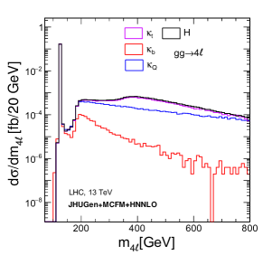
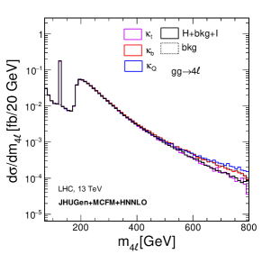
Figure 15: The invariant mass distribution of four-lepton ($4\ell=2e2\mu$) events produced through gluon fusion at the LHC with a 13 TeV proton collision energy. The different CP-even anomalous $Hgg$ couplings are simulated with JHUGen+MCFM at LO in QCD, and the NNLO $k$ factor is calculated with the HNNLO program, assuming signal and background $k$ factors to be the same as for the SM $H$ boson. Four off-shell scenarios are shown with the couplings chosen to match the SM on-shell $gg\to H\to 4\ell$ cross section: SM (solid black), top-quark only (magenta), bottom-quark only (red), and a point-like effective interaction (blue) shown in Eq. (37). The left plot shows the $gg\to H\to 4\ell$ process with only signal, while the right plot includes interference with the SM $gg\to 4\ell$ background, which is also shown separately in the dotted histogram.

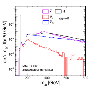
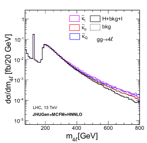
Figure 16: The four-lepton invariant mass distributions in gluon fusion production as in Fig. 15, but with the three CP-odd anomalous couplings instead, also chosen to match the SM on-shell $gg\to H\to 4\ell$ cross section.

VII.1 Off-shell effects due to Hgg anomalous couplings

The off-shell production of the $H$ boson may provide a way to disentangle contributions to the gluon fusion loop from either SM-like couplings to the top and bottom quarks, CP-odd couplings of the $H$ boson, or new heavy particles. We illustrate this in Fig. 15 for CP-even couplings and in Fig. 16 for CP-odd couplings. In order to illustrate the effects, we separate the signal contributions from the top quark, the bottom quark, and an effective point-like interaction, with both CP-even and CP-odd couplings to the $H$ boson. For illustration, the SM values of the $HVV$ couplings and of the $H$ boson width $\Gamma_{\rm tot}$ are assumed, but variations of these couplings are considered in Section VII.2, and a simultaneous measurement with $\Gamma_{\rm tot}$ can be considered. The tools allow the modeling of the gluon fusion loop with all possible couplings contributing simultaneously, including interference with the background $gg\to 4\ell$ process. The effective point-like interaction is equivalent to heavy $t^{\prime}$ and $b^{\prime}$ quarks in the loop, and this can also be configured in the JHU generator, with adjustable masses of the these new particles in the loop.

While in Section VI it was shown how the CP-even and CP-odd couplings in the gluon fusion loop can be separated by analyzing of on-shell $H$ boson production in association with two jets, this approach does not allow us to resolve different contributions to the loop. Off-shell production provides a way to separate those contributions. As can be seen in Figs. 15 and 16, the top quark contribution has a distinctive threshold enhancement around $2m_{t}$, with somewhat different behavior of the CP-even and CP-odd components. The heavy particle contribution proceeds without the $2m_{t}$ threshold, and the light particle contribution is highly suppressed. Therefore, the off-shell spectrum can be used to resolve the loop effects, such as to differentiate between the top quark and heavy BSM contributions in the loop or to set limits on the light quark Yukawa couplings or other possible light contributions, similarly to the techniques using the on-shell $H$ boson transverse momentum deFlorian:2016spz ; Bishara:2016jga . In all cases, the CP-odd component’s interference with the background is zero when integrated over the other observables. The actual analysis of the data will benefit from employing the full kinematics using the matrix-element approach.

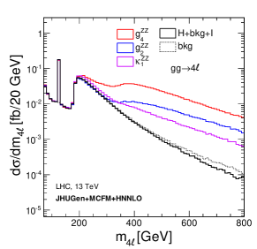
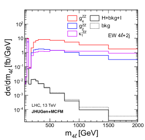
Figure 17: The four-lepton $4\ell$ invariant mass distributions in gluon fusion (left, $4\ell=2e2\mu$) and in associated electroweak production with two jets (right, $\ell=e,\mu,\tau$) at the LHC with a 13 TeV proton collision energy. The anomalous $HVV$ couplings are simulated with JHUGen+MCFM at LO in QCD, with the gluon fusion simulation settings and k factors matching those for SM in Fig. 15. Three anomalous $HVV$ couplings are modeled with coupling values chosen to match the SM on-shell $gg\to H\to 2e2\mu$ cross section. Interference with the SM $gg\to 4\ell$ (left) and electroweak (right) background is included.

VII.2 Off-shell effects due to HVV anomalous couplings

The off-shell production of the $H$ boson also allows testing the anomalous $HVV$ couplings of the $H$ boson to two electroweak bosons, $VV=WW,ZZ,Z\gamma,\gamma\gamma$. These couplings appear in the decay $H\to 4f$ in the gluon fusion process and in both production and decay in the electroweak process. The latter includes both VBF and $VH$ production, and in all cases interference with the gluon fusion or electroweak background is included. Examples of such a simulation are shown in Fig. 17. Three anomalous couplings are shown for illustration, $g_{4}^{ZZ}=g_{4}^{WW}$, $g_{2}^{ZZ}=g_{2}^{WW}$, and $\kappa_{1,2}^{ZZ}=\kappa_{1,2}^{WW}$, which involve interplay of either the $H$ boson or the $Z$ ($W$) boson going off shell. The anomalous couplings of the $H$ boson to the photon are not enhanced off-shell and are not shown here, but can be considered in analysis. Therefore, it is important to stress here that it is natural to use the physical Higgs basis in the EFT analysis of the off-shell region, since the behavior of the couplings involving the photon is drastically different.

Examples of applications of the tools developed here, both simulation and MELA discriminants, can be found in Refs. Sirunyan:2019twz ; Cepeda:2019klc where simultaneous analysis of the $H$ boson width and the couplings is performed both with the current LHC data and in projection to the HL-LHC. For example, with 3000 fb of data, a single LHC experiment is expected to constrain $\Gamma_{\rm tot}=4.1^{+1.1}_{-1.1}$ MeV, as shown in Fig. 106 of Ref. Cepeda:2019klc . With the current data sample from the LHC experiments, the off-shell region significantly improves the anomalous coupling constraints, even with $\Gamma_{\rm tot}$ profiled Sirunyan:2019twz . This is evident from the enhancement observed in Fig. 17. The expected gain is not as large at the HL-LHC, as Fig. 39 of Ref. Cepeda:2019klc shows, because with access to smaller couplings, the electroweak VBF and $VH$ production in the on-shell region plays a more important role.

It has been pointed out Azatov:2014jga ; Azatov:2016xik that the $gg\to 4\ell$ process also provides good sensitivity for constraining the top quark electroweak couplings. Similarly, gluon fusion in $ZH$ production is sensitive to the same top quark couplings and can be used to constrain them Bylund:2016phk ; Englert:2016hvy . In this work, however, we separate anomalous $H$ boson couplings from the rest of the electroweak interactions where this is possible in a consistent way. For the above cases, separating the effects is certainly possible, because top quark electroweak couplings can also be probed in e.g. $pp\to t\bar{t}Z$, which is independent of the Higgs sector. Moreover, there are no EFT relations between electroweak top quark couplings and $H$ boson couplings. However, the gauge boson self-interactions and the $H$ boson couplings cannot be separated if the EFT relations Eqs. (22–27) are applied in continuum electroweak production. We can account for these relations as discussed in the following Section VII.3.

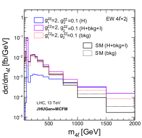
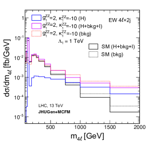
Figure 18: The four-lepton invariant mass distributions in $4\ell$ ($\ell=e,\mu,\tau$) associated electroweak production with two jets at the LHC with a 13 TeV proton collision energy. The anomalous $HVV$ couplings are simulated with JHUGen+MCFM. The black distributions show two SM scenarios: background only (dashed) and the full contribution including the $H$ boson (solid). The colored curves show an additional non-zero anomalous contribution from either $g_{2}^{ZZ}$ (left) or $\kappa_{1,2}^{ZZ}$ (right) in the $H$ boson production component (blue solid), in the background-only component (red dashed), and including all contributions (magenta solid).

VII.3 Off-shell effects due to gauge boson self-interactions

In Sections VII.1 and VII.2, only modifications of the $H$ boson couplings to either strong or weak gauge bosons are considered, and the background contributions in either $gg\to 4f$ or continuum electroweak production are assumed to be SM-like. However, as discussed in Section II, there is an intricate interplay between gauge boson self-couplings and $H$ boson gauge couplings. Therefore, under the EFT relationship, the $HVV$ anomalous contribution would affect the triple and quartic gauge boson self-couplings according to Eqs. (22–27). Figure 18 shows examples of the $m_{4\ell}$ distributions with anomalous gauge boson self-interactions in the EFT framework. These examples show the CP-conserving anomalous $g_{2}^{ZZ}$ and $\kappa_{1,2}^{ZZ}$ couplings, which are modified in Eqs. (17–21) for the $H$ boson couplings and in Eqs. (22–27) for the gauge boson self-couplings, keeping all the other anomalous couplings at zero. The size of the anomalous contribution is taken to be similar to the current constraints on anomalous $H$ boson couplings Sirunyan:2019twz from LHC measurements. It is evident from Fig. 18 that the resonant and nonresonant contributions are of similar size in electroweak production and that there is a sizable interference between the two. While current analyses of LHC data typically consider the $H$ boson couplings and gauge boson self-interactions separately Sirunyan:2019twz , the unified framework will allow future joint constraints.

VIII Application to the ZH process at next-to-leading order

Production of the $H$ boson in association with an electroweak gauge boson is known for its clean experimental signature and its excellent sensitivity to the $HVV$ couplings. During Run-II of the LHC, the experimental precision of $ZH$ analyses Khachatryan:2016vau ; Sirunyan:2018koj ; Aad:2019mbh ; Sirunyan:2018kst ; Aaboud:2018zhk has reached a level of accuracy that requires theory simulation beyond leading order. Therefore, we account for the dominant perturbative corrections at next-to-leading order QCD in this work and make them available in the JHUGen framework.

In addition to reducing theoretical uncertainties, the simulation at higher orders also reveals sensitivity to $H$ boson couplings that are invisible at the lowest order. In $ZH$ production, the $gg\to ZH$ sub-process enters for the first time through one-loop diagrams. The box diagram contribution in Fig. 4 yields sensitivity to the $H\!f\!\bar{f}$ couplings $\kappa_{f}$ and $\tilde{\kappa}_{f}$ in Eq. (2), which are screened in the $q\bar{q}$ production process.

We must stress that whenever we work with $ZH$ production, $\gamma H$ and $\gamma^{*}H$ production are equally important. This allows us to set constraints on anomalous $H\gamma\gamma$ and $HZ\gamma$ couplings, and we provide this functionality in the JHUGen framework.

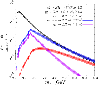
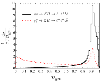
Figure 19: Distribution of the $m_{ZH}$ invariant mass (left) and ${\cal D}_{\rm ggZH}$ discriminant (right) in $gg$ and $q\bar{q}\to ZH\to\ell^{-}\ell^{+}b\bar{b}$ processes under the SM hypothesis in 14 TeV LHC collisions, with several components isolated for illustration. The left plot shows the differential cross section for the $q\bar{q}\to ZH$ process at both LO and NLO in QCD.

In Fig. 19 we show the SM $m_{ZH}$ distribution assuming the decays $Z\to\ell^{+}\ell^{-}$ and $H\to b\bar{b}$ at the $14$ TeV LHC. Contributions from $q\bar{q}$ and $gg$ initial states are shown separately, as are the triangle and box diagram parts of the $gg$ partonic process, shown in Fig. 4. The widths of the bands correspond to systematic uncertainties from varying the scale by a factor of two around its central value $\mu_{0}=m_{ZH}$. Close to the production threshold at $m_{ZH}=m_{Z}+m_{H}\approx 220$ GeV, the $q\bar{q}$ initial state dominates the cross section. Above the $2\,m_{t}\approx 345$ GeV energy, the top-quark induced $gg$ initial state becomes much more relevant. In particular, the triangle loop contribution, shown in blue, becomes as large as the $q\bar{q}$ contribution, shown in black, and even exceeds it at very high energies. However, as can be seen from the purple band in Fig. 19 the quantum interference between the triangle and box diagrams is strongly destructive and reduces the overall $gg$ contribution significantly. For this reason, the $gg$ contribution plays only a marginal role in the SM description of the $ZH$ process.

However, in anomalous coupling studies of physics beyond the SM, this strong destructive interference can be perturbed and lead to significantly larger cross sections. Hence, it is a sensitive probe of modifications from the SM. The $gg\to ZH$ process has yet another interesting feature. A superficial inspection of the triangle loop contribution in Fig. 19 suggests sensitivity to the $HVV$ couplings in Eq. (1). Yet, an explicit calculation shows that the contributions from $g_{2}^{VV}$ and $g_{4}^{VV}$ drop out and yield a zero contribution to the complete squared one-loop amplitude. Moreover, both the triangle and the box diagrams are only sensitive to the axial-vector coupling of the gauge boson to the fermions in the loop. Hence, photons do not couple to the closed fermion loop. The process $gg\to\gamma H$ can only proceed through an intermediate $Z^{*}$, which decays into $\gamma H$ via the $\kappa_{2}^{Z\gamma}$ coupling in Eq. (1). Obviously, $gg\to WH$ does not exist because of charge conservation. The absence of sensitivity to anomalous $HVV$ couplings $g_{2}^{VV}$ and $g_{4}^{VV}$ does not render the $gg\to ZH$ process completely irrelevant to their study. If we assume, for example, that the $HZZ$ interaction involves non-zero $g_{2}^{ZZ}$, which does not contribute to the triangle diagrams, the pattern of destructive interference with the box diagram would change. Hence, there is a strong sensitivity to the $HVV$ couplings, which is entangled with possible anomalous values of the $H\!f\!\bar{f}$ couplings.

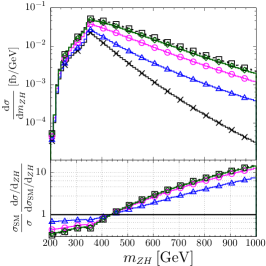
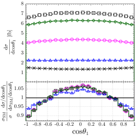
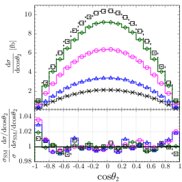
Figure 20: Kinematic distributions for simulated $gg\to ZH\to\ell^{-}\ell^{+}b\bar{b}$ events at 14 TeV for several scenarios: $\kappa=1,\tilde{\kappa}=0$ (SM, black crosses); $\kappa=-1,\tilde{\kappa}=0$ (black boxes); $\kappa=0,\tilde{\kappa}=\pm 1$ (magenta circles); $\kappa=1/\sqrt{2},\tilde{\kappa}=\pm 1/\sqrt{2}$ (blue triangles); $\kappa=-1/\sqrt{2},\tilde{\kappa}=\pm 1/\sqrt{2}$ (green diamonds).

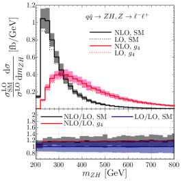
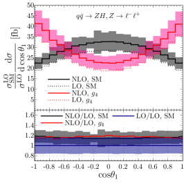
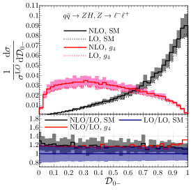
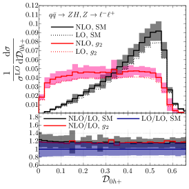
Figure 21: Selected kinematic distributions for simulated $q\bar{q}\to ZH\to\ell^{-}\ell^{+}b\bar{b}$ events at 14 TeV shown at LO (dotted) and NLO (solid) in QCD. The SM (black) and anomalous coupling model (red) are shown. The anomalous coupling model shown is the pseudoscalar model $f_{g4}=1$ in all plots except for the ${\cal D}_{0h+}$ discriminant distribution, where the $f_{g2}=1$ model is shown instead. The bottom panels show the $k$-factor ratios.

The above mentioned special features of the loop-induced $gg$ process motivate separating it from the $q\bar{q}$ production mode. While it is not feasible to isolate one process from the other on an event-by-event basis, it is possible to enhance (or decrease) the relative fraction of the two processes. We use the MELA approach with the ${\cal{D}_{\rm ggZH}}$ discriminant calculated according to Eq. (44) with ${\rm sig}=gg\to ZH$ and ${\rm alt}=q\bar{q}\to ZH$. The distributions of ${\cal{D}_{\rm ggZH}}$ for the $gg$- and $q\bar{q}$-initiated processes are shown in Fig. 19. As an example, in a restricted range of the ${\cal{D}_{\rm ggZH}}$ observable which keeps 80% of the $gg$-initiated process, the fraction of this process is enhanced from 7% to 22%. As described in Section V, this approach is superior to selection based on individual kinematic observables, such as selecting higher values of $m_{ZH}$ or $p_{\mathrm{T}}^{H}$ Hespel-2015-gg .

In the following, we present anomalous coupling results for the $gg$ and $q\bar{q}$ processes separately. This serves to illustrate the particular anomalous coupling features of our framework. A full experimental result needs to include both processes together. In Fig. 20, we show the effects of several combinations of anomalous $Ht\bar{t}$ couplings in the $gg\to ZH$ process and compare the shape changes to the SM prediction. We use the general interaction structure from Eq. (2) with CP-even ($\kappa$) and CP-odd ($\tilde{\kappa}$) Yukawa-type couplings and consider the scenarios with a wrong sign Yukawa coupling, pure CP-odd couplings, and mixtures of CP-even and CP-odd couplings. In Fig. 20, we show the $ZH$ invariant mass and the two angles $\theta_{1}$ and $\theta_{2}$. The angles are defined for the $VH$ process in Fig. 5 and Ref. Anderson:2013afp , but we note that it is possible to define the sign of $\cos\theta_{1}$ when $\theta_{1}$ is the angle between the $Z$ boson and the longitudinal direction of the overall boost of the $V^{*}\to ZH$ system, defined in the $V^{*}$ rest frame. In the case where the $VH$ system has finite transverse momentum, we first boost the system in the transverse direction to set the transverse motion to zero. For a practical application of this approach at the LHC, see Ref. (Chatrchyan:2011ya, ).

In the upper row of Fig. 21 we present the $q\bar{q}\to ZH$ process and compare the leading order with the next-to-leading QCD prediction. The black and red curves correspond to the SM $HZZ$ coupling and a pure CP-odd coupling from $g_{4}^{ZZ}$ in Eq. (1), respectively. Shape changes due to the different coupling structure are significant, even on a logarithmic scale. Hence, this process offers strong discrimination power even for small admixtures of $g_{4}^{ZZ}$ into the SM-like $g_{1}^{ZZ}$ coupling structure. The higher order corrections, shown in the differences between the solid and dotted curves and in the lower panes, are positive, fairly constant, and $\mathcal{O}(+10\%)$. In the lower row of Fig. 21 we show the matrix element discriminants ${\cal D}_{0h+}$ and ${\cal D}_{0-}$, defined in Eq. (44), for the alternative hypotheses $g_{2}^{ZZ}=1$ and $g_{4}^{ZZ}=1$, respectively. Again, the NLO QCD corrections are fairly constant over a wide range. The plots show strong discrimination power between each anomalous hypothesis and the SM. The results allow for a more accurate estimate of systematic uncertainties in future analyses, and the flat correction reinforces previous leading order studies.

IX Application to new resonance production

The techniques developed for the study of the $H(125)$ boson would apply to a search for or a study of a new resonance $X(m_{X})$ which may arise in the extensions of the SM, such as any Singlet model or Two Higgs Doublet model. For example, if any enhancement or modification of the di-boson spectrum or kinematics in the off-shell region is observed, one would have to determine the source of this effect. For example, it might come from a modification of the $H$ boson couplings in the off-shell region, including anomalous tensor structures; a modification of the continuum production, possibly from anomalous self-interactions; or yet another resonance $X$ with a larger mass. This latter scenario is necessary to consider in order to complete the experimental studies.

If a new state $X$ is observed, one would need to determine its spin and parity quantum numbers in all accessible final states. The techniques discussed in Section VI would be directly relevant. If the width of the resonance is sizable, interference with background, as discussed in Section VII, will become relevant. Moreover, interference with the off-shell $H(125)$ boson tail would become important as well. All these effects are included in the coherent framework of the JHU generator with the modified MCFM matrix element library, and are available in the MELA package for MC re-weighting and optimal discriminant calculations. They have been employed in analyses of Run-II of LHC data Sirunyan:2018qlb ; Sirunyan:2019pqw .

Applications of off-shell $H(125)$ simulation with an additional broad $X(m_{X})$ resonance are shown in Figs. 22, 23, and 24. The cross section of the generated resonance $X$ corresponds to the limit obtained by the recent CMS search Sirunyan:2018qlb , which includes all interference effects of a broad resonance. The most general $XVV$ and $Xgg$ couplings discussed in application to $HVV$ and $Hgg$ in Sections VI and VII are possible. It is interesting to observe that in the scalar case, the interference of $X(m_{X})$ with the $H(125)$ off-shell tail and its interference with the background have opposite signs and partially cancel each other, but the net effect still remains and alters the distributions. In the cases of anomalous $XVV$ couplings, the size of the interference changes, and in some particular cases, such as the $g_{4}$ coupling, even the sign of the interference flips. The point-like $Xgg$ couplings are also tested and shown in Fig. 23, which models the scenario when new heavy states in the gluon fusion loop are responsible for production of the new state $X$.

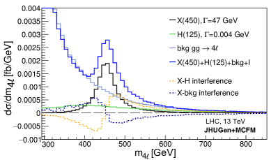
Figure 22: Differential cross section of the gluon fusion process $gg\to ZZ/Z\gamma^{*}/\gamma^{*}\gamma^{*}\to 4\ell$ as a function of invariant mass $m_{4\ell}$ generated with JHUGen+MCFM at LO in QCD. The distribution is shown in the presence of a hypothetical scalar $X(450)$ resonance with SM-like couplings, $m_{X}=450$ GeV, and $\Gamma_{X}=47$ GeV. Several components are either isolated or combined as indicated in the legend. Interference (I) of all contributing amplitudes is included.

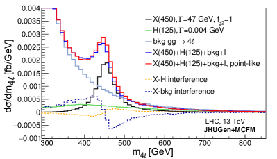
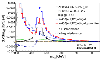
Figure 23: Same as Fig. 22, but for the anomalous couplings of a new resonance $X(450)$. A scalar resonance with $f_{g2}=1$ (left) and a pseudoscalar resonance with $f_{g4}=1$ (right) are considered. Both a top loop and a point-like interaction are considered in the gluon fusion production.

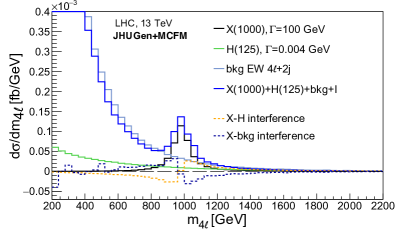
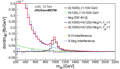
Figure 24: Differential cross section of the electroweak production process $qq\to qq(ZZ/Z\gamma^{*}/\gamma^{*}\gamma^{*}\to 4\ell)$ as a function of invariant mass $m_{4\ell}$ generated with JHUGen+MCFM. The distribution is shown in the presence of a hypothetical $X(1000)$ resonance with SM-like couplings (left) and anomalous couplings ($f_{g2}=1$ and $f_{g4}=1$, right), $m_{X}=1000$ GeV, and $\Gamma_{X}=100$ GeV. Several components are either isolated or combined as indicated in the legend. Interference (I) of all contributing amplitudes is included.

X Summary

In this paper, we have investigated the Higgs boson interactions at invariant masses both at and well beyond the mass peak. We considered the weak vector boson fusion process $pp\to 4f+jj$, gluon fusion $pp\to 4f$, and associated production $pp\to VH$. All three processes contribute to both the on-shell and off-shell signal regions. NLO QCD effects, including the $gg$ initial state, are investigated in $pp\to VH$ production. Through these processes, we study $HVV$ interactions in the regime of large momentum transfer, which exposes the unitarization feature in the Standard Model and is sensitive to the mechanism of electroweak symmetry breaking at high energies. Our framework allows a general coupling parameterization for the 125 GeV Higgs boson and for a possible second spin-zero resonance. Modifications of the triple and quartic gauge boson couplings are also considered. Deviations from the SM expectation can be parameterized in terms of anomalous couplings, effective field theory operators, and pseudo observables. The framework of the JHUGen event generator and MELA library for the matrix element analysis enable simulation, optimal discrimination, reweighting techniques, and analysis with the most general anomalous couplings of a bosonic resonance and the triple and quartic gauge boson interactions. The capabilities of the framework have been illustrated with projections for measuring the EFT operators with the expected full data samples of the LHC and the High-Luminosity LHC.

Acknowledgments: We acknowledge the contributions of CMS collaboration colleagues to the MELA project development and help with integration and validation of the JHU event generator. We thank Tianran Chen for updating the Hom4PS program for this analysis and providing support, we thank Amitabh Basu for suggesting the cutting planes algorithm in application to our analysis, we thank Michael Spira and Margarete Mühlleitner for help with the HDECAY and C2HDM_HDECAY programs, we thank Andrew Gilbert for help with features of the Root program, we thank Giovanni Petrucciani for discussion of the Higgs cross section studies, we thank Jared Feingold for machine learning studies, we thank Savvas Kyriacou for help with the fit implementation, and we thank Jeffrey Davis for help in cross section calculations and interface to different coupling conventions in the generator. This research is partially supported by the U.S. NSF under grants PHY-1404302 and PHY-1707887, by the Fundamental Research Funds for the Central Universities (China), and by the U.S. DOE under grant DE-SC0011702. Calculations reported in this paper were performed on the Maryland Advanced Research Computing Center (MARCC).

Note added: A new application of this framework to LHC data appeared in Ref. CMS-HIG-19-009 . We would also like to point that the relative sign of the CP-even and CP-odd couplings in Eq. (37) is consistent with Refs. Chetyrkin:1996ke ; Chetyrkin:1998mw ; Bernreuther:2015fts , while the sign was reversed between Refs. Artoisenet:2013puc ; Demartin:2014fia . We adopt the sign convention of the antisymmetric tensor $\varepsilon_{0123}=+1$ consistent with Refs. Chetyrkin:1996ke ; Chetyrkin:1998mw ; Bernreuther:2015fts and thank Werner Bernreuther for pointing out the sign ambiguity.

Appendix A Coupling relation to the Warsaw basis

Translations of the EFT operators between the Higgs basis and the Warsaw basis, which is defined in Ref. Grzadkowski:2010es , can be performed with tools such as Rosetta Falkowski:2015wza . For example, under the assumption that $\delta c_{z}=\delta c_{w}$ in Section II, we have five independent CP-even and three CP-odd electroweak $HVV$ operators, as well as one CP-even and one CP-odd $Hgg$ operator in the Higgs basis. The same number of independent $H$ boson operators exists in the Warsaw basis. The relationship between the six CP-even operators is quoted explicitly in Eq. (14) of Ref. Falkowski:2015wza . Eliminating the assumption $\delta c_{z}=\delta c_{w}$ yields one additional degree of freedom: $\delta m$ in the Higgs basis; $\Delta M_{W}$ in our anomalous coupling approach in Eq. (17); and a linear combination of three coefficients, called $\delta v$ in Ref. Falkowski:2015wza , in the Warsaw basis.

We extend the above equivalence to include the CP-odd operators and derive the translation of the four operators between the Higgs basis and the Warsaw basis as

$$g_{4}^{ZZ} = -2\frac{v^{2}}{\Lambda^{2}}\left(s_{w}^{2}w_{\phi\tilde{B}}+c_{w}^{2}w_{\phi\tilde{W}}+s_{w}c_{w}w_{\phi B\tilde{W}}\right)\,,$$

$$g_{4}^{\gamma\gamma} = -2\frac{v^{2}}{\Lambda^{2}}\left(c_{w}^{2}w_{\phi\tilde{B}}+s_{w}^{2}w_{\phi\tilde{W}}-s_{w}c_{w}w_{\phi B\tilde{W}}\right)\,,$$

$$g_{4}^{Z\gamma} = -2\frac{v^{2}}{\Lambda^{2}}\left(s_{w}c_{w}(w_{\phi\tilde{W}}-w_{\phi\tilde{B}})+\frac{1}{2}(s_{w}^{2}-c_{w}^{2})w_{\phi B\tilde{W}}\right)\,,$$

$$g_{4}^{gg} = -2\frac{v^{2}}{\Lambda^{2}}w_{\phi\tilde{G}}\,.$$ (50)

Another set of coefficients is sometimes used and is related to the Warsaw basis through

$$C_{\varphi\tilde{B}} = -\frac{c_{w}^{2}}{\Lambda^{2}e^{2}}w_{\phi\tilde{B}}\,,$$

$$C_{\varphi\tilde{W}} = -\frac{s_{w}^{2}}{\Lambda^{2}e^{2}}w_{\phi\tilde{W}}\,,$$

$$C_{\varphi B\tilde{W}} = -\frac{s_{w}c_{w}}{\Lambda^{2}e^{2}}w_{\phi B\tilde{W}}\,,$$

$$C_{\varphi\tilde{G}} = -\frac{w_{\phi\tilde{G}}}{\Lambda^{2}g_{s}^{2}}\,.$$ (51)

We would like to note that it is a question of convenience which operators in the Higgs basis are chosen as independent ones under the SU(2)$\times$U(1) symmetry. For studies performed in this paper, we find it convenient to pick $\delta c_{z},c_{zz},c_{z\Box},\tilde{c}_{zz},c_{z\gamma},\tilde{c}_{z\gamma},c_{\gamma\gamma},\tilde{c}_{\gamma\gamma},c_{gg},$ and $\tilde{c}_{gg}$ as an independent set of $HVV$ and $Hgg$ couplings and use Eqs. (17–21) to express the other couplings listed in Eq. (II.1). In other analyses, another convention may be more convenient. For instance, when performing measurements with the $WW$ final state, one could pick $\delta c_{w},c_{ww},c_{w\Box},$ and $\tilde{c}_{ww}$ in place of $\delta c_{z},c_{zz},c_{z\Box},$ and $\tilde{c}_{zz}$ to perform the measurements, and express the latter using Eqs. (17)–(20). In the end, all couplings can be translated into a common convention. In order to simplify translation between different coupling conventions and operator bases, including the Higgs and Warsaw bases, within the JHU generator framework, we provide the JHUGenLexicon program, which includes an interface to the generator and matrix element library and can also be used for standalone or other applications.

References

- (1) Y. Gao et al., “Spin determination of single-produced resonances at hadron colliders”, Phys. Rev. D 81 (2010) 075022, doi:10.1103/PhysRevD.81.075022, arXiv:1001.3396.
- (2) S. Bolognesi et al., “Spin and parity of a single-produced resonance at the LHC”, Phys. Rev. D 86 (2012) 095031, doi:10.1103/PhysRevD.86.095031, arXiv:1208.4018.
- (3) I. Anderson et al., “Constraining anomalous HVV interactions at proton and lepton colliders”, Phys. Rev. D 89 (2014) 035007, doi:10.1103/PhysRevD.89.035007, arXiv:1309.4819.
- (4) A. V. Gritsan, R. Röntsch, M. Schulze, and M. Xiao, “Constraining anomalous Higgs boson couplings to the heavy flavor fermions using matrix element techniques”, Phys. Rev. D 94 (2016) 055023, doi:10.1103/PhysRevD.94.055023, arXiv:1606.03107.
- (5) J. M. Campbell and R. K. Ellis, “MCFM for the Tevatron and the LHC”, Nucl. Phys. Proc. Suppl. 205-206 (2010) 10–15, doi:10.1016/j.nuclphysbps.2010.08.011, arXiv:1007.3492.
- (6) J. M. Campbell, R. K. Ellis, and C. Williams, “Vector boson pair production at the LHC”, JHEP 07 (2011) 018, doi:10.1007/JHEP07(2011)018, arXiv:1105.0020.
- (7) J. M. Campbell, R. K. Ellis, and C. Williams, “Bounding the Higgs width at the LHC using full analytic results for ”, JHEP 04 (2014) 060, doi:10.1007/JHEP04(2014)060, arXiv:1311.3589.
- (8) J. M. Campbell and R. K. Ellis, “Higgs constraints from vector boson fusion and scattering”, JHEP 04 (2015) 030, doi:10.1007/JHEP04(2015)030, arXiv:1502.02990.
- (9) J. M. Campbell, R. K. Ellis, and W. T. Giele, “A Multi-Threaded Version of MCFM”, Eur. Phys. J. C 75 (2015) 246, doi:10.1140/epjc/s10052-015-3461-2, arXiv:1503.06182.
- (10) C. A. Nelson, “Correlation between decay planes in Higgs-boson decays into a W Pair (into a Z Pair)”, Phys. Rev. D 37 (1988) 1220, doi:10.1103/PhysRevD.37.1220.
- (11) A. Soni and R. M. Xu, “Probing CP violation via Higgs decays to four leptons”, Phys. Rev. D 48 (1993) 5259, doi:10.1103/PhysRevD.48.5259, arXiv:hep-ph/9301225.
- (12) T. Plehn, D. L. Rainwater, and D. Zeppenfeld, “Determining the structure of Higgs couplings at the LHC”, Phys. Rev. Lett. 88 (2002) 051801, doi:10.1103/PhysRevLett.88.051801, arXiv:hep-ph/0105325.
- (13) S. Y. Choi, D. J. Miller, M. M. Mühlleitner, and P. M. Zerwas, “Identifying the Higgs spin and parity in decays to Z pairs”, Phys. Lett. B 553 (2003) 61, doi:10.1016/S0370-2693(02)03191-X, arXiv:hep-ph/0210077.
- (14) C. P. Buszello, I. Fleck, P. Marquard, and J. J. van der Bij, “Prospective analysis of spin- and CP-sensitive variables in at the LHC”, Eur. Phys. J. C 32 (2004) 209, doi:10.1140/epjc/s2003-01392-0, arXiv:hep-ph/0212396.
- (15) V. Hankele, G. Klamke, D. Zeppenfeld, and T. Figy, “Anomalous Higgs boson couplings in vector boson fusion at the CERN LHC”, Phys. Rev. D 74 (2006) 095001, doi:10.1103/PhysRevD.74.095001, arXiv:hep-ph/0609075.
- (16) E. Accomando et al., “Workshop on CP studies and non-standard Higgs physics”, (2006). arXiv:hep-ph/0608079.
- (17) R. M. Godbole, D. J. Miller, and M. M. Mühlleitner, “Aspects of CP violation in the HZZ coupling at the LHC”, JHEP 12 (2007) 031, doi:10.1088/1126-6708/2007/12/031, arXiv:0708.0458.
- (18) K. Hagiwara, Q. Li, and K. Mawatari, “Jet angular correlation in vector-boson fusion processes at hadron colliders”, JHEP 07 (2009) 101, doi:10.1088/1126-6708/2009/07/101, arXiv:0905.4314.
- (19) A. De Rújula et al., “Higgs look-alikes at the LHC”, Phys. Rev. D 82 (2010) 013003, doi:10.1103/PhysRevD.82.013003, arXiv:1001.5300.
- (20) N. D. Christensen, T. Han, and Y. Li, “Testing CP Violation in ZZH Interactions at the LHC”, Phys. Lett. B 693 (2010) 28, doi:10.1016/j.physletb.2010.08.008, arXiv:1005.5393.
- (21) J. Ellis, D. S. Hwang, V. Sanz, and T. You, “A fast track towards the ‘Higgs’ spin and parity”, JHEP 11 (2012) 134, doi:10.1007/JHEP11(2012)134, arXiv:1208.6002.
- (22) Y. Chen, N. Tran, and R. Vega-Morales, “Scrutinizing the Higgs signal and background in the golden channel”, JHEP 01 (2013) 182, doi:10.1007/JHEP01(2013)182, arXiv:1211.1959.
- (23) P. Artoisenet et al., “A framework for Higgs characterisation”, JHEP 11 (2013) 043, doi:10.1007/JHEP11(2013)043, arXiv:1306.6464.
- (24) M. Chen et al., “Role of interference in unraveling the ZZ couplings of the newly discovered boson at the LHC”, Phys. Rev. D 89 (2014) 034002, doi:10.1103/PhysRevD.89.034002, arXiv:1310.1397.
- (25) F. Maltoni, K. Mawatari, and M. Zaro, “Higgs characterisation via vector-boson fusion and associated production: NLO and parton-shower effects”, Eur. Phys. J. C 74 (2014) 2710, doi:10.1140/epjc/s10052-013-2710-5, arXiv:1311.1829.
- (26) A. Azatov, C. Grojean, A. Paul, and E. Salvioni, “Taming the off-shell Higgs boson”, Zh. Eksp. Teor. Fiz. 147 (2015) 410–425, doi:10.1134/S1063776115030140,10.7868/S0044451015030039, arXiv:1406.6338. [J. Exp. Theor. Phys.120,354(2015)].
- (27) G. Cacciapaglia, A. Deandrea, G. Drieu La Rochelle, and J.-B. Flament, “Higgs couplings: disentangling New Physics with off-shell measurements”, Phys. Rev. Lett. 113 (2014) 201802, doi:10.1103/PhysRevLett.113.201802, arXiv:1406.1757.
- (28) A. Denner, S. Dittmaier, S. Kallweit, and A. Mück, “HAWK 2.0: A Monte Carlo program for Higgs production in vector-boson fusion and Higgs strahlung at hadron colliders”, Comput. Phys. Commun. 195 (2015) 161–171, doi:10.1016/j.cpc.2015.04.021, arXiv:1412.5390.
- (29) M. J. Dolan, P. Harris, M. Jankowiak, and M. Spannowsky, “Constraining -violating Higgs sectors at the LHC using gluon fusion”, Phys. Rev. D 90 (2014) 073008, doi:10.1103/PhysRevD.90.073008, arXiv:1406.3322.
- (30) C. Englert, Y. Soreq, and M. Spannowsky, “Off-Shell Higgs Coupling Measurements in BSM scenarios”, JHEP 05 (2015) 145, doi:10.1007/JHEP05(2015)145, arXiv:1410.5440.
- (31) M. Gonzalez-Alonso, A. Greljo, G. Isidori, and D. Marzocca, “Pseudo-observables in Higgs decays”, Eur. Phys. J. C 75 (2015) 128, doi:10.1140/epjc/s10052-015-3345-5, arXiv:1412.6038.
- (32) A. Ballestrero and E. Maina, “Interference Effects in Higgs production through Vector Boson Fusion in the Standard Model and its Singlet Extension”, JHEP 01 (2016) 045, doi:10.1007/JHEP01(2016)045, arXiv:1506.02257.
- (33) A. Greljo, G. Isidori, J. M. Lindert, and D. Marzocca, “Pseudo-observables in electroweak Higgs production”, Eur. Phys. J. C 76 (2016) 158, doi:10.1140/epjc/s10052-016-4000-5, arXiv:1512.06135.
- (34) B. Hespel, F. Maltoni, and E. Vryonidou, “Higgs and Z boson associated production via gluon fusion in the SM and the 2HDM”, JHEP 06 (2015) 065, doi:10.1007/JHEP06(2015)065, arXiv:1503.01656.
- (35) N. Kauer, C. O’Brien, and E. Vryonidou, “Interference effects for and searches in gluon fusion at the LHC”, JHEP 10 (2015) 074, doi:10.1007/JHEP10(2015)074, arXiv:1506.01694.
- (36) N. Kauer and C. O’Brien, “Heavy Higgs signal–background interference in in the Standard Model plus real singlet”, Eur. Phys. J. C 75 (2015) 374, doi:10.1140/epjc/s10052-015-3586-3, arXiv:1502.04113.
- (37) W. Kilian, T. Ohl, J. Reuter, and M. Sekulla, “Resonances at the LHC beyond the Higgs boson: The scalar/tensor case”, Phys. Rev. D 93 (2016) 036004, doi:10.1103/PhysRevD.93.036004, arXiv:1511.00022.
- (38) K. Mimasu, V. Sanz, and C. Williams, “Higher Order QCD predictions for Associated Higgs production with anomalous couplings to gauge bosons”, JHEP 08 (2016) 039, doi:10.1007/JHEP08(2016)039, arXiv:1512.02572.
- (39) C. Degrande et al., “Electroweak Higgs boson production in the standard model effective field theory beyond leading order in QCD”, Eur. Phys. J. C 77 (2017) 262, doi:10.1140/epjc/s10052-017-4793-x, arXiv:1609.04833.
- (40) S. Dwivedi, D. K. Ghosh, B. Mukhopadhyaya, and A. Shivaji, “Distinguishing -odd couplings of the Higgs boson to weak boson pairs”, Phys. Rev. D 93 (2016) 115039, doi:10.1103/PhysRevD.93.115039, arXiv:1603.06195.
- (41) LHC Higgs Cross Section Working Group Collaboration, “Handbook of LHC Higgs Cross Sections: 4. Deciphering the Nature of the Higgs Sector”, doi:10.23731/CYRM-2017-002, arXiv:1610.07922.
- (42) A. Azatov, C. Grojean, A. Paul, and E. Salvioni, “Resolving gluon fusion loops at current and future hadron colliders”, JHEP 09 (2016) 123, doi:10.1007/JHEP09(2016)123, arXiv:1608.00977.
- (43) A. Denner, J.-N. Lang, and S. Uccirati, “NLO electroweak corrections in extended Higgs Sectors with RECOLA2”, JHEP 07 (2017) 087, doi:10.1007/JHEP07(2017)087, arXiv:1705.06053.
- (44) N. Deutschmann, C. Duhr, F. Maltoni, and E. Vryonidou, “Gluon-fusion Higgs production in the Standard Model Effective Field Theory”, JHEP 12 (2017) 063, doi:10.1007/JHEP12(2017)063,10.1007/JHEP02(2018)159, arXiv:1708.00460. [Erratum: JHEP02,159(2018)].
- (45) A. Greljo et al., “Electroweak Higgs production with HiggsPO at NLO QCD”, Eur. Phys. J. C 77 (2017) 838, doi:10.1140/epjc/s10052-017-5422-4, arXiv:1710.04143.
- (46) D. Goncalves, T. Plehn, and J. M. Thompson, “Weak boson fusion at 100 TeV”, Phys. Rev. D 95 (2017) 095011, doi:10.1103/PhysRevD.95.095011, arXiv:1702.05098.
- (47) B. Jäger, L. Salfelder, M. Worek, and D. Zeppenfeld, “Physics opportunities for vector-boson scattering at a future 100 TeV hadron collider”, Phys. Rev. D 96 (2017) 073008, doi:10.1103/PhysRevD.96.073008, arXiv:1704.04911.
- (48) S. Brass et al., “Transversal Modes and Higgs Bosons in Electroweak Vector-Boson Scattering at the LHC”, Eur. Phys. J. C 78 (2018) 931, doi:10.1140/epjc/s10052-018-6398-4, arXiv:1807.02512.
- (49) R. Gomez-Ambrosio, “Studies of Dimension-Six EFT effects in Vector Boson Scattering”, Eur. Phys. J. C 79 (2019) 389, doi:10.1140/epjc/s10052-019-6893-2, arXiv:1809.04189.
- (50) D. Gonçalves, T. Han, and S. Mukhopadhyay, “Higgs Couplings at High Scales”, Phys. Rev. D 98 (2018) 015023, doi:10.1103/PhysRevD.98.015023, arXiv:1803.09751.
- (51) R. V. Harlander, J. Klappert, C. Pandini, and A. Papaefstathiou, “Exploiting the WH/ZH symmetry in the search for New Physics”, Eur. Phys. J. C 78 (2018) 760, doi:10.1140/epjc/s10052-018-6234-x, arXiv:1804.02299.
- (52) R. V. Harlander, J. Klappert, S. Liebler, and L. Simon, “vh@nnlo-v2: New physics in Higgs Strahlung”, JHEP 05 (2018) 089, doi:10.1007/JHEP05(2018)089, arXiv:1802.04817.
- (53) S. J. Lee, M. Park, and Z. Qian, “Probing unitarity violation in the tail of the off-shell Higgs boson in mode”, Phys. Rev. D 100 (2019) 011702, doi:10.1103/PhysRevD.100.011702, arXiv:1812.02679.
- (54) J. Kalinowski et al., “Same-sign WW scattering at the LHC: can we discover BSM effects before discovering new states?”, Eur. Phys. J. C 78 (2018) 403, doi:10.1140/epjc/s10052-018-5885-y, arXiv:1802.02366.
- (55) G. Perez, M. Sekulla, and D. Zeppenfeld, “Anomalous quartic gauge couplings and unitarization for the vector boson scattering process ”, Eur. Phys. J. C 78 (2018) 759, doi:10.1140/epjc/s10052-018-6230-1, arXiv:1807.02707.
- (56) M. Jaquier and R. Röntsch, “Mixed scalar-pseudoscalar Higgs boson production through next-to-next-to-leading order at the LHC”, JHEP 06 (2020) 005, doi:10.1007/JHEP06(2020)005, arXiv:1911.10631.
- (57) A. Denner, S. Dittmaier, and A. Mück, “PROPHECY4F 3.0: A Monte Carlo program for Higgs-boson decays into four-fermion final states in and beyond the Standard Model”, Comput. Phys. Commun. 254 (2020) 107336, doi:10.1016/j.cpc.2020.107336, arXiv:1912.02010.
- (58) S. Banerjee et al., “Towards the ultimate differential SMEFT analysis”, arXiv:1912.07628.
- (59) CMS Collaboration, “Observation of a new boson at a mass of 125 GeV with the CMS experiment at the LHC”, Phys. Lett. B 716 (2012) 30–61, doi:10.1016/j.physletb.2012.08.021, arXiv:1207.7235.
- (60) CMS Collaboration, “Study of the Mass and Spin-Parity of the Higgs Boson Candidate Via Its Decays to Z Boson Pairs”, Phys. Rev. Lett. 110 (2013) 081803, doi:10.1103/PhysRevLett.110.081803, arXiv:1212.6639.
- (61) CMS Collaboration, “Measurement of the properties of a Higgs boson in the four-lepton final state”, Phys. Rev. D 89 (2014) 092007, doi:10.1103/PhysRevD.89.092007, arXiv:1312.5353.
- (62) CMS Collaboration, “Measurement of Higgs boson production and properties in the WW decay channel with leptonic final states”, JHEP 01 (2014) 096, doi:10.1007/JHEP01(2014)096, arXiv:1312.1129.
- (63) ATLAS Collaboration, “Evidence for the spin-0 nature of the Higgs boson using ATLAS data”, Phys. Lett. B 726 (2013) 120–144, doi:10.1016/j.physletb.2013.08.026, arXiv:1307.1432.
- (64) CMS Collaboration, “Constraints on the Higgs boson width from off-shell production and decay to Z-boson pairs”, Phys. Lett. B 736 (2014) 64, doi:10.1016/j.physletb.2014.06.077, arXiv:1405.3455.
- (65) CMS Collaboration, “Observation of the diphoton decay of the Higgs boson and measurement of its properties”, Eur. Phys. J. C 74 (2014) 3076, doi:10.1140/epjc/s10052-014-3076-z, arXiv:1407.0558.
- (66) CMS Collaboration, “Constraints on the spin-parity and anomalous HVV couplings of the Higgs boson in proton collisions at 7 and 8 TeV”, Phys. Rev. D 92 (2015) 012004, doi:10.1103/PhysRevD.92.012004, arXiv:1411.3441.
- (67) CMS Collaboration, “Limits on the Higgs boson lifetime and width from its decay to four charged leptons”, Phys. Rev. D 92 (2015) 072010, doi:10.1103/PhysRevD.92.072010, arXiv:1507.06656.
- (68) CMS Collaboration, “Search for a Higgs boson in the mass range from 145 to 1000 GeV decaying to a pair of W or Z bosons”, JHEP 10 (2015) 144, doi:10.1007/JHEP10(2015)144, arXiv:1504.00936.
- (69) ATLAS Collaboration, “Study of the spin and parity of the Higgs boson in diboson decays with the ATLAS detector”, Eur. Phys. J. C 75 (2015) 476, doi:10.1140/epjc/s10052-015-3685-1, arXiv:1506.05669.
- (70) CMS Collaboration, “Combined search for anomalous pseudoscalar HVV couplings in VH(H ) production and H VV decay”, Phys. Lett. B 759 (2016) 672, doi:10.1016/j.physletb.2016.06.004, arXiv:1602.04305.
- (71) CMS Collaboration, “Constraints on anomalous Higgs boson couplings using production and decay information in the four-lepton final state”, Phys. Lett. B 775 (2017) 1, doi:10.1016/j.physletb.2017.10.021, arXiv:1707.00541.
- (72) CMS Collaboration, “Constraints on anomalous couplings from the production of Higgs bosons decaying to lepton pairs”, Phys. Rev. D 100 (2019) 112002, doi:10.1103/PhysRevD.100.112002, arXiv:1903.06973.
- (73) CMS Collaboration, “Measurements of the Higgs boson width and anomalous HVV couplings from on-shell and off-shell production in the four-lepton final state”, Phys. Rev. D 99 (2019) 112003, doi:10.1103/PhysRevD.99.112003, arXiv:1901.00174.
- (74) CMS Collaboration, “Measurements of H production and the CP structure of the Yukawa interaction between the Higgs boson and top quark in the diphoton decay channel”, Phys. Rev. Lett. 125 (2020) 061801, doi:10.1103/PhysRevLett.125.061801, arXiv:2003.10866.
- (75) CMS Collaboration, “Search for a new scalar resonance decaying to a pair of Z bosons in proton-proton collisions at TeV”, JHEP 06 (2018) 127, doi:10.1007/JHEP06(2018)127,10.1007/JHEP03(2019)128, arXiv:1804.01939. [Erratum: JHEP03,128(2019)].
- (76) CMS Collaboration, “Search for a heavy Higgs boson decaying to a pair of W bosons in proton-proton collisions at 13 TeV”, arXiv:1912.01594.
- (77) M. Cepeda et al., “Higgs Physics at the HL-LHC and HE-LHC”, CERN Yellow Rep. Monogr. 7 (2019) 221–584, doi:10.23731/CYRM-2019-007.221, arXiv:1902.00134.
- (78) ATLAS, CMS Collaboration, “Measurements of the Higgs boson production and decay rates and constraints on its couplings from a combined ATLAS and CMS analysis of the LHC pp collision data at and 8 TeV”, JHEP 08 (2016) 045, doi:10.1007/JHEP08(2016)045, arXiv:1606.02266.
- (79) CMS Collaboration, “Combined measurements of Higgs boson couplings in proton-proton collisions at ”, Eur. Phys. J. C 79 (2019) 421, doi:10.1140/epjc/s10052-019-6909-y, arXiv:1809.10733.
- (80) ATLAS Collaboration, “Combined measurements of Higgs boson production and decay using up to fb-1 of proton-proton collision data at 13 TeV collected with the ATLAS experiment”, Phys. Rev. D 101 (2020) 012002, doi:10.1103/PhysRevD.101.012002, arXiv:1909.02845.
- (81) CMS Collaboration, “Observation of Higgs boson decay to bottom quarks”, Phys. Rev. Lett. 121 (2018) 121801, doi:10.1103/PhysRevLett.121.121801, arXiv:1808.08242.
- (82) ATLAS Collaboration, “Observation of decays and production with the ATLAS detector”, Phys. Lett. B 786 (2018) 59–86, doi:10.1016/j.physletb.2018.09.013, arXiv:1808.08238.
- (83) CMS Collaboration, “Observation of H production”, Phys. Rev. Lett. 120 (2018) 231801, doi:10.1103/PhysRevLett.120.231801, arXiv:1804.02610.
- (84) ATLAS Collaboration, “Observation of Higgs boson production in association with a top quark pair at the LHC with the ATLAS detector”, Phys. Lett. B 784 (2018) 173–191, doi:10.1016/j.physletb.2018.07.035, arXiv:1806.00425.
- (85) CMS Collaboration, “Observation of the Higgs boson decay to a pair of leptons with the CMS detector”, Phys. Lett. B 779 (2018) 283–316, doi:10.1016/j.physletb.2018.02.004, arXiv:1708.00373.
- (86) ATLAS Collaboration, “Cross-section measurements of the Higgs boson decaying into a pair of -leptons in proton-proton collisions at TeV with the ATLAS detector”, Phys. Rev. D 99 (2019) 072001, doi:10.1103/PhysRevD.99.072001, arXiv:1811.08856.
- (87) “JHU generator”,. http://spin.pha.jhu.edu/.
- (88) B. Grzadkowski, M. Iskrzynski, M. Misiak, and J. Rosiek, “Dimension-Six Terms in the Standard Model Lagrangian”, JHEP 10 (2010) 085, doi:10.1007/JHEP10(2010)085, arXiv:1008.4884.
- (89) A. Falkowski, “Higgs Basis: Proposal for an EFT basis choice for LHC HXSWG”, Technical Report LHCHXSWG-INT-2015-001, 2015. https://cds.cern.ch/record/2001958.
- (90) M. Gonzalez-Alonso, A. Greljo, G. Isidori, and D. Marzocca, “Electroweak bounds on Higgs pseudo-observables and decays”, Eur. Phys. J. C 75 (2015) 341, doi:10.1140/epjc/s10052-015-3555-x, arXiv:1504.04018.
- (91) A. Alboteanu, W. Kilian, and J. Reuter, “Resonances and Unitarity in Weak Boson Scattering at the LHC”, JHEP 11 (2008) 010, doi:10.1088/1126-6708/2008/11/010, arXiv:0806.4145.
- (92) N. Kauer and G. Passarino, “Inadequacy of zero-width approximation for a light Higgs boson signal”, JHEP 08 (2012) 116, doi:10.1007/JHEP08(2012)116, arXiv:1206.4803.
- (93) F. Caola and K. Melnikov, “Constraining the Higgs boson width with ZZ production at the LHC”, Phys. Rev. D 88 (2013) 054024, doi:10.1103/PhysRevD.88.054024, arXiv:1307.4935.
- (94) A. Djouadi, J. Kalinowski, M. Mühlleitner, and M. Spira, “HDECAY: Twenty++ years after”, Comput. Phys. Commun. 238 (2019) 214–231, doi:10.1016/j.cpc.2018.12.010, arXiv:1801.09506.
- (95) D. Fontes et al., “The C2HDM revisited”, JHEP 02 (2018) 073, doi:10.1007/JHEP02(2018)073, arXiv:1711.09419.
- (96) I. Brivio, T. Corbett, and M. Trott, “The Higgs width in the SMEFT”, JHEP 10 (2019) 056, doi:10.1007/JHEP10(2019)056, arXiv:1906.06949.
- (97) CMS Collaboration, “Updated results on the new boson discovered in the search for the standard model Higgs boson in the channel in pp collisions at = 7 and 8 TeV”, Technical Report CMS-HIG-12-041, CERN, Geneva, 2012.
- (98) S. Frixione, P. Nason, and C. Oleari, “Matching NLO QCD computations with Parton Shower simulations: the POWHEG method”, JHEP 11 (2007) 070, doi:10.1088/1126-6708/2007/11/070, arXiv:0709.2092.
- (99) LHC Higgs Cross Section Working Group Collaboration, “Handbook of LHC Higgs Cross Sections: 3. Higgs Properties”, doi:10.5170/CERN-2013-004, arXiv:1307.1347.
- (100) Particle Data Group Collaboration, “Review of Particle Physics”, Chin. Phys. C38 (2014) 090001, doi:10.1088/1674-1137/38/9/090001.
- (101) A. Denner, S. Dittmaier, and L. Hofer, “Collier: a fortran-based Complex One-Loop LIbrary in Extended Regularizations”, Comput. Phys. Commun. 212 (2017) 220–238, doi:10.1016/j.cpc.2016.10.013, arXiv:1604.06792.
- (102) J. Brehmer et al., “Effective LHC measurements with matrix elements and machine learning”, J. Phys. Conf. Ser. 1525 (2020) 012022, doi:10.1088/1742-6596/1525/1/012022, arXiv:1906.01578.
- (103) N. Berger et al., “Simplified Template Cross Sections - Stage 1.1”, arXiv:1906.02754.
- (104) J. Neyman and E. S. Pearson, “On the Problem of the Most Efficient Tests of Statistical Hypotheses”, Philosophical Transactions of the Royal Society A231 (1933) 289–337, doi:10.1098/rsta.1933.0009.
- (105) D. Atwood and A. Soni, “Analysis for magnetic moment and electric dipole moment form-factors of the top quark via ”, Phys. Rev. D 45 (1992) 2405–2413, doi:10.1103/PhysRevD.45.2405.
- (106) M. Davier, L. Duflot, F. Le Diberder, and A. Rouge, “The Optimal method for the measurement of tau polarization”, Phys. Lett. B 306 (1993) 411–417, doi:10.1016/0370-2693(93)90101-M.
- (107) M. Diehl and O. Nachtmann, “Optimal observables for the measurement of three gauge boson couplings in ”, Z. Phys. C62 (1994) 397–412, doi:10.1007/BF01555899.
- (108) A. Hocker et al., “TMVA - Toolkit for Multivariate Data Analysis”, arXiv:physics/0703039.
- (109) W. Verkerke and D. P. Kirkby, “The RooFit toolkit for data modeling”, in 13 International Conference for Computing in High-Energy and Nuclear Physics (CHEP03). 2003. arXiv:physics/0306116. CHEP-2003-MOLT007.
- (110) R. Brun and F. Rademakers, “ROOT: An object oriented data analysis framework”, Nucl. Instrum. Meth. A 389 (1997) 81, doi:10.1016/S0168-9002(97)00048-X.
- (111) T. Melia, P. Nason, R. Röntsch, and G. Zanderighi, “, and production, including /Z interference, singly resonant contributions and interference for identical leptons”, JHEP 1111 (2011) 078.
- (112) CMS Collaboration, “Measurements of properties of the Higgs boson in the four-lepton final state in proton-proton collisions at TeV”, Technical Report CMS-HIG-19-001, CERN, Geneva, 2019.
- (113) T. Sjöstrand et al., “An introduction to PYTHIA 8.2”, Comput. Phys. Commun. 191 (2015) 159, doi:10.1016/j.cpc.2015.01.024, arXiv:1410.3012.
- (114) T. Chen and T.-Y. Li, “Homotopy continuation method for solving systems of nonlinear and polynomial equations”, Commun. Inf. Syst. 15 (2015), no. 2, 119–307, doi:10.4310/CIS.2015.v15.n2.a1.
- (115) T. Chen, T.-L. Lee, and T.-Y. Li, “Hom4PS-3: A Parallel Numerical Solver for Systems of Polynomial Equations Based on Polyhedral Homotopy Continuation Methods”, in Mathematical Software—ICMS 2014, H. Hong and C. Yap, eds., number 8592 in Lecture Notes in Computer Science, pp. 183–190. Springer Berlin Heidelberg, January, 2014. doi:10.1007/978-3-662-44199-2_30.
- (116) T. Chen, T.-L. Lee, and T.-Y. Li, “Mixed cell computation in Hom4PS-3”, Journal of Symbolic Computation 79, Part 3 (March, 2017) 516–534, doi:10.1016/j.jsc.2016.07.017.
- (117) A. S. Nemirovsky and D. B. Yudin, “Problem complexity and method efficiency in optimization.”. Wiley, 1983.
- (118) Gurobi Optimization, LLC, “Gurobi Optimizer Reference Manual”, 2018.
- (119) S. Catani and M. Grazzini, “An NNLO subtraction formalism in hadron collisions and its application to Higgs boson production at the LHC”, Phys. Rev. Lett. 98 (2007) 222002, doi:10.1103/PhysRevLett.98.222002, arXiv:hep-ph/0703012.
- (120) M. Grazzini, “NNLO predictions for the Higgs boson signal in the and decay channels”, JHEP 02 (2008) 043, doi:10.1088/1126-6708/2008/02/043, arXiv:0801.3232.
- (121) M. Grazzini and H. Sargsyan, “Heavy-quark mass effects in Higgs boson production at the LHC”, JHEP 09 (2013) 129, doi:10.1007/JHEP09(2013)129, arXiv:1306.4581.
- (122) K. Melnikov and M. Dowling, “Production of two Z-bosons in gluon fusion in the heavy top quark approximation”, Phys. Lett. B 744 (2015) 43–47, doi:10.1016/j.physletb.2015.03.030, arXiv:1503.01274.
- (123) F. Caola, K. Melnikov, R. Röntsch, and L. Tancredi, “QCD corrections to ZZ production in gluon fusion at the LHC”, Phys. Rev. D 92 (2015) 094028, doi:10.1103/PhysRevD.92.094028, arXiv:1509.06734.
- (124) M. Grazzini, S. Kallweit, M. Wiesemann, and J. Y. Yook, “ production at the LHC: NLO QCD corrections to the loop-induced gluon fusion channel”, JHEP 03 (2019) 070, doi:10.1007/JHEP03(2019)070, arXiv:1811.09593.
- (125) F. Caola et al., “QCD corrections to vector boson pair production in gluon fusion including interference effects with off-shell Higgs at the LHC”, JHEP 07 (2016) 087, doi:10.1007/JHEP07(2016)087, arXiv:1605.04610.
- (126) F. Bishara, U. Haisch, P. F. Monni, and E. Re, “Constraining Light-Quark Yukawa Couplings from Higgs Distributions”, Phys. Rev. Lett. 118 (2017) 121801, doi:10.1103/PhysRevLett.118.121801, arXiv:1606.09253.
- (127) O. Bessidskaia Bylund et al., “Probing top quark neutral couplings in the Standard Model Effective Field Theory at NLO in QCD”, JHEP 05 (2016) 052, doi:10.1007/JHEP05(2016)052, arXiv:1601.08193.
- (128) C. Englert, R. Rosenfeld, M. Spannowsky, and A. Tonero, “New physics and signal-background interference in associated production”, EPL 114 (2016) 31001, doi:10.1209/0295-5075/114/31001, arXiv:1603.05304.
- (129) B. Hespel, F. Maltoni, and E. Vryonidou, “Higgs and Z boson associated production via gluon fusion in the SM and the 2HDM”, JHEP 06 (2015) 065, doi:10.1007/JHEP06(2015)065, arXiv:1503.01656.
- (130) CMS Collaboration, “Measurement of the weak mixing angle with the Drell-Yan process in proton-proton collisions at the LHC”, Phys. Rev. D 84 (2011) 112002, doi:10.1103/PhysRevD.84.112002, arXiv:1110.2682.
- (131) CMS Collaboration, “Constraints on anomalous Higgs boson couplings to vector bosons and fermions in production and decay in the channel”, Technical Report CMS-HIG-19-009, CERN, Geneva, 2020.
- (132) K. G. Chetyrkin, B. A. Kniehl, and M. Steinhauser, “Three loop O corrections to hadronic Higgs decays”, Nucl. Phys. B 490 (1997) 19, doi:10.1016/S0550-3213(97)00051-5, arXiv:hep-ph/9701277.
- (133) K. G. Chetyrkin, B. A. Kniehl, M. Steinhauser, and W. A. Bardeen, “Effective QCD interactions of CP odd Higgs bosons at three loops”, Nucl. Phys. B 535 (1998) 3, doi:10.1016/S0550-3213(98)00594-X, arXiv:hep-ph/9807241.
- (134) W. Bernreuther et al., “Production of heavy Higgs bosons and decay into top quarks at the LHC”, Phys. Rev. D 93 (2016), no. 3, 034032, doi:10.1103/PhysRevD.93.034032, arXiv:1511.05584.
- (135) F. Demartin et al., “Higgs characterisation at NLO in QCD: CP properties of the top-quark Yukawa interaction”, Eur. Phys. J. C74 (2014), no. 9, 3065, doi:10.1140/epjc/s10052-014-3065-2, arXiv:1407.5089.
- (136) A. Falkowski et al., “Rosetta: an operator basis translator for Standard Model effective field theory”, Eur. Phys. J. C 75 (2015) 583, doi:10.1140/epjc/s10052-015-3806-x, arXiv:1508.05895.