Speeding up the AIFV-$2$ dynamic programs by two orders of magnitude using Range Minimum Queries

Abstract

AIFV-$2$ codes are a new method for constructing lossless codes for memoryless sources that provide better worst-case redundancy than Huffman codes. They do this by using two code trees instead of one and also allowing some bounded delay in the decoding process. Known algorithms for constructing AIFV-code are iterative; at each step they replace the current code tree pair with a “better” one. The current state of the art for performing this replacement is a pair of Dynamic Programming (DP) algorithms that use $O(n^{5})$ time to fill in two tables, each of size $O(n^{3})$ (where $n$ is the number of different characters in the source).

This paper describes how to reduce the time for filling in the DP tables by two orders of magnitude, down to $O(n^{3})$. It does this by introducing a grouping technique that permits separating the $\Theta(n^{3})$-space tables into $\Theta(n)$ groups, each of size $O(n^{2})$, and then using Two-Dimensional Range-Minimum Queries (RMQs) to fill in that group’s table entries in $O(n^{2})$ time. This RMQ speedup technique seems to be new and might be of independent interest.

1 Introduction

Almost Instantaneous Fixed to Variable-$2$ (AIVF-$2$) codes were introduced recently in a series of papers [9, 10, 14, 15]

Similar to Huffman Codes, these provide lossless encoding for a fixed probabilistic memoryless source. They differ from Huffman codes in that they use a pair of coding trees instead of just one tree, sometimes coding using the first and sometimes using the second. They also no longer provide instantaneous decoding. Instead, decoding might require a bounded delay. That is, it might be necessary to read up to $2$ extra characters after a codeword ends before certifying the the completion (and decoding) of the codeword. The advantage of AIFV-$2$ codes over Huffman codes is that they guarantee redundancy of at most $1/2$ instead of the redundancy of $1$ guaranteed by Huffman encoding [9].

The procedure for constructing optimal (min-redundancy) AIFV-$2$ codes is much more complicated than that of finding Huffman codes. It is an iterative one that, at each step, replaces the current pair of coding trees by a new, better, pair. The original paper [15] only proved that its iterative algorithm terminated. This was improved to polynomial time steps by [7], which used only $O(b)$ iterations, where $b$ is the maximum number of bits used to encode one of the input source probabilities.

Each iterative step of [15]’s algorithm was originally implemented using an exponential time Integer Linear Program. This was later improved by [10] to $O(n^{5})$ time, using Dynamic Programming (DP) to replace the ILP. $n$ is the number of different characters in the original souce.

The purpose of this paper is to show how the DP method can be sped up to $O(n^{3})$ time. Combined with [7], this yields a $O(n^{3}b)$ time algorithm for constructing AIFV-$2$ codes.

Historically, there have been two major approaches to speeding up DPs. The first is the Knuth-Yao Quadrangle-Inequality method [11, 12, 16, 17]. The second is the use of “monotonicity” or the “Monge Property” and the application of the SMAWK [1] algorithm [3, Section 3.8] ([13] provides a good example of this approach). There are also variations, e.g., [5], that while not exactly one or the other, share many of their properties. [2] provides a recent overview of the techniques available.

Both methods improve running times by “grouping” calculations. More specifically, they all essentially fill in a DP table of size $\Theta(n^{k})$, for some $k$, in which calculating an individual table entry requires $\Theta(n)$ work. Thus, a-priori, filling in the table seems to require $\Theta(n^{k+1})$ time. The speedups work by grouping the entries in sets of size $\Theta(n)$ and calculating all entries in the group in $\Theta(n)$ time. The Quadrangle-Inequality approach does this via amortization while the SMAWK approach does this by a transformation into another problem (matrix row-minima calculation). Both approaches lead to a $\Theta(n)$ speedup, permitting filling in the table in an optimal $\Theta(n^{k})$ time.

Both DPs in [10] have $O(n^{3})$ size tables with each entry requiring $\Theta(n^{2})$ individual evaluation time, leading to the $O(n^{5})$ time algorithms. The main contribution of this paper is the development of new grouping techniques that permit speeding up the DPs by $\Theta(n^{2}),$ decreasing the running times to $O(n^{3}).$

More specifically, the table entries are now partitioned into $\Theta(n)$ groups, each containing $\Theta(n^{2})$ entries. For each group, a $\Theta(n)\times\Theta(n)$ sized rectangular matrix $M$ is then built; calculating the value of each table entry in the group is shown to be equivalent to performing a Two-Dimensional Range Minimum (2D RMQ) query on $M$ (along with $O(1)$ extra work). Known results [18] on 2D RMQ queries imply that $O(n^{2})$ queries can be inplemented using a total of $O(n^{2})$ time. Thus all entries in each group of size $\Theta(n^{2})$ can be evaluated in $O(n^{2})$ time, leading to an $O(n^{3})$ time algorithm.

To the best of our knowledge this is the first time 2D RMQs have been used for speeding up Dynamic Programming in this fashion, so this technique might be of independent interest.

Section 2 quickly reviews known facts about 2D RMQs. It also introduces the two specialized versions of RMQs that will be needed and shows that they can be solved even more simply (practically) than standard RMQs. Section 3 is the main result of the paper. It states (before derivation) the two DPs of interest and then describes the new technique to reduce their evaluation from $\Theta(n^{5})$ to $\Theta(n^{3}).$ The remainder of the paper then provides the backstory. Section 4 defines the motivating AIVF-$2$ problem and the technique for solving it. Finally, Section 5 describes the derivation of the AIFV-$2$ DPs that were solved in Section 3. We emphasize that while these DPs are not exactly the ones introduced in [10] they are very similar and were derived using the same observations and basic tools (the top-down signature technique of [6, 4]). The derivation of these new DPs was necessary, though. Their slightly different structure is what permits successfully applying the 2D RMQ technique to them

We conclude by noting that AIFV-$2$ codes were later extended to AIFV-$m$ codes by [9]. These replace the pair of coding trees by an $m$-tuple. The iterative algorithms for constructing these codes use $O(n^{2m+1})$ time DP algorithms that fill in size $O(n^{m+1})$ DP tables as subroutines. An interesting direction for future work is whether it is possible to reduce the running times of evaluating those DP tables by a factor of $\Theta(n^{m})$ via the use of the corresponding $m$D RMQ algorithms from [18]. This would require a much better understanding of the structure of those DPs in [9] than currently exist.

2 Range Minimum Queries

As, mentioned, the speedup in evaluating the DPs will result from grouping and then using Range Minimum Queries (RMQs). This section quickly reviews facts about RMQs for later use.

Definition 1 (2D RMQ).

Let $M=(M_{i,j})$ be a given $m\times n$ matrix; $0\leq i\leq m,$ $0\leq j\leq n$. The two-dimensional range minimum query (2D RMQ) problem is, for $0\leq a_{1}\leq a_{2}\leq n$ and $0\leq b_{1}\leq b_{2}\leq n$ to return the value

$$RMQ(M:a_{1},a_{2},b_{1},b_{2})\triangleq\min\{M_{i,j}\,:\,a_{1}\leq i\leq a_{2},\,b_{1}\leq j\leq b_{2}\}.$$

and indices $i^{\prime},j^{\prime}$, $a_{1}\leq i^{\prime}\leq a_{2},$ $b_{1}\leq j^{\prime}\leq b_{2}$ such that

$$M_{i^{\prime},j^{\prime}}=RMQ(M:a_{1},a_{2},b_{1},b_{2}).$$

This can be solved using

Lemma 1 ([18]).

Let $M=(M_{i,j})$ be a given $m\times n$ matrix; $0\leq i\leq m,$ $0\leq j\leq n$. There is an $O(mn)$ time algorithm to preprocess $M$ that permits answering any subsequent 2D RMQ query in $O(1)$ time.

While theoretically optimal, the algorithm in [18] is quite complicated. To make the speed up more practical to implement, we note in advance that all of the RMQ queries used later will be one of the two following specialized types:

Definition 2.

Let $M=(M_{i,j})$ be a given $m\times n$ matrix; $0\leq i\leq m,$ $0\leq j\leq n$. Let $0\leq a\leq m,$ $0\leq b\leq n$. See Figure 1.

• Define a restricted column query as

  $$RCQ(M:a,b)\triangleq RMQ(M:a,m,b,b).$$

• Define a restricted RMQ query as

  $$RRMQ(M:a,b)\triangleq RMQ(M:a,m,0,b).$$

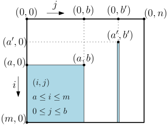
Figure 1: Illustration of Definition 2. $M$ is an $(m+1)\times(n+1)$ matrix. $RCQ(M:a^{\prime},b^{\prime})$ is the minimum of the entries in the long thin blue column descending down from $(a^{\prime},b^{\prime}).$ $RRMQ(M:a,b)$ is the minimum of the entries in the blue rectangle with upper-right corner $(a,b)$.

Directly from the definition,

$$\forall b,\quad RCQ(M:a,b)=\begin{cases}M_{m,b}&\mbox{if $a=m$},\\ \min\left(M_{a,b},RCQ(M:a+1,b)\right)&\mbox{if $a<m$}.\end{cases}$$

Thus, the values of all of the $\Theta(mn)$ possible $RCQ(M:a,b)$ queries (and the associated indices at which minimization occurs) can be easily calculated in $\Theta(mn)$ time.

Also directly from the definitions,

$$RRMQ(M:a,b)=\begin{cases}RCQ(M:a,0)&\mbox{if $b=0$},\\ \min\left(RRMQ(M:a,b-1),RCQ(M:a,b)\right)&\mbox{if $b>0$.}\\ \end{cases}$$

Thus, assuming that all of the $RCQ(M:a,b)$ have been precalculated, the values of all of the $\Theta(mn)$ possible $RRMQ(M:a,b)$ queries (and the associated indices at which minimization occurs) can also be easily calculated in $\Theta(mn)$ time.

For later use we collect this in a lemma.

Lemma 2.

Let $M$ be a given $m\times n$ matrix; $0\leq i\leq m,$ $0\leq j\leq n$. There is an $O(mn)$ time algorithm that calculates the answers to all of the possible $RCQ(M:a,b)$ and $RRMQ(M:a,b)$ queries.

3 The Dynamic Program and its speedup

Definition 3.

Let $p_{1},\ldots,p_{n}$ be given such that $\forall i,\,p_{i}>0$ and $\sum_{i=1}^{n}p_{i}=1.$ Set

$$W_{m}\triangleq\sum_{j\leq m}p_{j},\quad\mbox{and}\quad W^{\prime}_{m}\triangleq\sum_{j>m}p_{j}=1-W_{m}$$

and, for $m^{\prime}<m$,

$$W_{m^{\prime},m}\triangleq\sum_{m^{\prime}<j\leq m}p_{j}=W_{m}-W_{m^{\prime}}.$$

The algorithm precalculates and stores all of the $W_{m}$ in $O(n)$ time. Subsequently, the $W_{m},$ $W^{\prime}_{m}$ and $W_{m^{\prime},m}$ can all be calculated in $O(1)$ time.

The Dynamic Programs are defined on $O(n^{3})$ size tables that are indexed by Signatures. The next two definitions define the Signature set (of indices) and the Dynamic Programming recurrence imposed on them.

Definition 4 (The Signature Set and costs).

Let $C$ ($0\leq C\leq 1$) be fixed.

• Define

  $${\cal S}_{n}\triangleq\left\{(m;p;z)\,:\,\mbox{$0\leq z\leq m\leq n$ and $0\leq p\leq n$}\right\}$$

  to be the signature set for the problem of size $n.$

• Let $(m^{\prime};p^{\prime};z^{\prime})\not=(m,p,z)\in{\cal S}_{n}$.
  We say $(m^{\prime};p^{\prime};z^{\prime})$ can be expanded into $(m;p;z)$, denoted by

  $$(m^{\prime};p^{\prime};z^{\prime})\rightarrow(m,p,z),$$

  if there exists $e_{0},e_{1}$ satisfying

  $$e_{0},\,e_{1}\geq 0\quad\mbox{ \rm such that }\quad 0\leq e_{0}+e_{1}\leq p^{\prime}$$ (1)

  and

  $$m = m^{\prime}+e_{0}+e_{1},$$ (2)

  $$z = e_{1},$$ (3)

  $$p = z^{\prime}+2(p^{\prime}-e_{0}-e_{1}).$$ (4)

• For $\alpha\in{\cal S}_{n}$, define the immediate predecessor set of $\alpha$ to be

  $$P(\alpha)\triangleq\{\alpha^{\prime}\in{\cal S}_{n}\,:\,\alpha^{\prime}\rightarrow\alpha\}.$$

• Let $\alpha_{1},\alpha_{2}\in{\cal S}_{n}.$ We say that $\alpha_{1}$ leads to $\alpha_{2}$, denoted by $\alpha_{1}\rightsquigarrow\alpha_{2}$, if there exists a path from $\alpha_{1}$ to $\alpha_{2}$ using “$\rightarrow$”.

• Let $I\subset{\cal S}_{n}$ and $\alpha\in{\cal S}_{n}$. We say that $I\rightsquigarrow\alpha$ if $\alpha\not\in I$ and there exists $\alpha^{\prime}\in I$ such that $\alpha^{\prime}\rightsquigarrow\alpha$.

• Let $\alpha^{\prime}=(m^{\prime};p^{\prime};z^{\prime})$ and $\alpha=(m,p;z)$ where $\alpha^{\prime}\rightarrow\alpha$. The associated expansion costs are

  $$c_{0}(\alpha^{\prime},\,\alpha) \triangleq W^{\prime}_{m^{\prime}}+CW_{m^{\prime}-z^{\prime},m^{\prime}},$$

  $$c_{1}(\alpha^{\prime},\,\alpha) \triangleq W^{\prime}_{m^{\prime}}-CW_{m^{\prime},m-z}.$$

The two dynamic programs used in the construction of AIFV-$2$ codes are given in the next definition.

Definition 5 (The $\mathrm{OPT}_{s}(\alpha)$ tables).

• Let $I_{0}\subset{\cal S}_{n}$ be a given initial set (independent of $n$) for the $\mathrm{OPT}_{0}$ table with known values $\bar{c}_{0}(\alpha)$ for $\alpha\in I_{0}.$ Now define

  $$\mathrm{OPT}_{0}(\alpha)=\begin{cases}\bar{c}_{0}(\alpha)&\mbox{if $\alpha\in I_{0}$}\\ \min_{\alpha^{\prime}\in P(\alpha)}\{\mathrm{OPT}_{0}(\alpha^{\prime})+c_{0}(\alpha^{\prime},\alpha)\}&\mbox{if $I_{0}\rightsquigarrow\alpha$}\\ \infty&\mbox{otherwise}\end{cases}$$

• Let $I_{1}\subset{\cal S}_{n}$ be a given initial set (independent of $n$) for the $\mathrm{OPT}_{1}$ table with known values $\bar{c}_{1}(\alpha)$ for $\alpha\in I_{1}.$ Now define

  $$\mathrm{OPT}_{1}(\alpha)=\begin{cases}\bar{c}_{1}(\alpha)&\mbox{if $\alpha\in I_{1}$}\\ \min_{\alpha^{\prime}\in P(\alpha)}\{\mathrm{OPT}_{1}(\alpha^{\prime})+c_{1}(\alpha^{\prime},\alpha)\}&\mbox{if $I_{1}\rightsquigarrow\alpha$}\\ \infty&\mbox{otherwise}\end{cases}$$

• Furthermore, for $s\in\{0,1\},$ for $\alpha\not\in I_{s}$ with $I_{s}\rightsquigarrow\alpha$, set

  $$\mathrm{Pred}_{s}(\alpha)\triangleq\operatorname*{\arg\!\min}_{\alpha^{\prime}\in P(\alpha)}\{\mathrm{OPT}_{s}(\alpha^{\prime})+c_{s}(\alpha^{\prime},\alpha)\}$$

The $\bar{c}_{s}(\alpha)$ for $\alpha\in I_{s}$ are the initial conditions for the corresponding dynamic programs.

For intuition, let $G_{s}(n)$ be the directed graph with vertices $\alpha\in{\cal S}_{n}$ with the cost of edge $(\alpha^{\prime},\,\alpha)$ being the expansion cost $c_{s}(\alpha^{\prime},\,\alpha)$ except that edges from $(0;0;0)$ to $\alpha\in I_{s}$ have cost $\bar{c}_{s}(\alpha)$ and edges that are not expansions have costs set to $\infty.$ Then $\mathrm{OPT}_{s}(\alpha)$ is just the cost of the shortest path from $(0;0;0)$ to $\alpha$ in $G_{s}(n).$ The actual path could be found by following the $\mathrm{Pred}_{s}(\alpha)$ pointers backward from $\alpha$. By definition, the expansion costs $c_{s}(\alpha^{\prime},\,\alpha)$ are all non-negative, so the $\mathrm{OPT}_{s}(\alpha)$ values are all well-defined.

The next set of lemmas will imply that $G_{s}(n)$ is a Directed Acyclic Graph so the recurrences define a Dynamic Program. They will also suggest an efficient grouping mechanism, leading to fast evaluation.

Lemma 3.

Let $(m^{\prime};p^{\prime};z^{\prime}),(m;z;p)\in\mathcal{S}_{n}.$ Then

$$(m^{\prime};p^{\prime};z^{\prime})\rightarrow(m,z,p)$$

if and only if all of

$$2m^{\prime}+2p^{\prime}+z^{\prime} = 2m+p,$$ (5)

$$m^{\prime}+p^{\prime} \geq m,$$ (6)

$$m^{\prime} \leq m-z,$$ (7)

$$(p^{\prime},z^{\prime}) \not= (0,0),$$ (8)

are satisfied.

Proof.

First assume that $(m^{\prime};p^{\prime};z^{\prime})\rightarrow(m,p,z)$.

Let $e_{0},e_{1}$ be the unique pair that satisfies (1)-(4). Then (5) follows from

$$2m^{\prime}+2p^{\prime} = 2(m-e_{0}-e_{1})+(p-z^{\prime}+2e_{0}+2e_{1})$$

$$= 2m+p-z^{\prime};$$

(6) follows from

$$m^{\prime}+p^{\prime}\geq m^{\prime}+e_{0}+e_{1}=m;$$

(7) follows from

$$m-z=m-e_{1}=m^{\prime}-e_{0}\geq m^{\prime}.$$

(8) follows from the fact that the combination of $(p^{\prime},z^{\prime})=(0,0)$ and Equation 4 would imply $p=-(e_{0}+e_{1})$. Since $p\geq 0$, this further implies $e_{0}=e_{1}=0$ and thus $m=m^{\prime}$ and $p=z=0$. This would contradict $(m^{\prime};z^{\prime};p^{\prime})\not=(m;z;p).$

For the other direction assume that Equations (5)-(8) all hold. We will show that Equations (1)-(4) with $(m^{\prime};z^{\prime};p^{\prime})\not=(m;z;p)$ also all hold with $e_{0}=m-m^{\prime}-z$ and $e_{1}=z$. Equations (2) and (3) are trivially satisfied. (4) follows from

$$p = 2m^{\prime}+2p^{\prime}+z^{\prime}-2m$$

$$= z^{\prime}-2(m-m^{\prime})+2p^{\prime}$$

$$= z^{\prime}-2(e_{0}+e_{1})+2p^{\prime}$$

$$= z^{\prime}+2(p^{\prime}-e_{0}-e_{1}).$$

Next note that $e_{1}=z\geq 0$ and, from (5) and (7), $e_{0}=m-z-m^{\prime}\geq 0$. Finally, from from (6), $p^{\prime}\geq m-m^{\prime}=e_{0}+e_{1}$ so Equation 1 holds.

It only remains to show that $(m^{\prime};z^{\prime};p^{\prime})\not=(m;z;p).$ Suppose, not and $(m^{\prime};z^{\prime};p^{\prime})=(m;z;p).$ Then from (4), $e_{0}=e_{1}=0$ so from (3) $z^{\prime}=z=0$ and thus from (4), $p=2p^{\prime}$ implying $p^{\prime}=p=0.$ But this contradicts (8). ∎

Definition 6.

For $d\geq 0$, define

$${\cal I}(d) \triangleq \{(m;p;z)\in{\cal S}_{n}\,:\,2m+p=d\},$$

$${\cal I}^{\prime}(d) \triangleq \{(m^{\prime};p^{\prime};z^{\prime})\in{\cal S}_{n}\,:\,2m^{\prime}+2p^{\prime}+z^{\prime}=d\ \mbox{and}\ (p^{\prime},z^{\prime})\not=(0,0)\}.$$

Now note that Lemma 3 can be rewritten as

Corollary 1.

If $\alpha\in{\cal I}(d)$ then

$$P(\alpha)=\Bigl{\{}(m^{\prime};p^{\prime};z^{\prime})\in{\cal I}^{\prime}(d))\,:\,m^{\prime}+p^{\prime}\geq m\mbox{ and }m^{\prime}\leq m-z\Bigr{\}}\subseteq{\cal I}^{\prime}(d)).$$

Next note

Lemma 4.

Let $d>0.$ Then

$${\cal I}^{\prime}(d)\subseteq\bigcup_{d^{\prime}<d}{\cal I}(d^{\prime}).$$ (9)

Proof.

Let $\alpha=(m^{\prime},p^{\prime},z^{\prime})\in{\cal I}^{\prime}(d).$ Since the ${\cal I}(d^{\prime})$ partition ${\cal S}_{n}$, there must exist some $d^{\prime}$ such that $\alpha\in{\cal I}(d^{\prime}).$ Suppose that $d\leq d^{\prime}.$ Then

$$2m^{\prime}+2p^{\prime}+z^{\prime}=d\leq d^{\prime}=2m^{\prime}+p^{\prime},$$

implying $p^{\prime}+z^{\prime}\leq 0$ so $(p,z)=(0,0)$, contradicting the definition of ${\cal I}^{\prime}(d)).$ Thus $d^{\prime}<d.$ Since this is true for all $\alpha\in{\cal I}^{\prime}(d),$ Equation 9 follows. ∎

Corollary 1 and Lemma 4 together imply that the $\mathrm{OPT}_{s}(\alpha)$ tables can be evaluated in the order $\alpha\in{\cal I}(d)$ for $d=1,2,3\ldots$. This ordering guarantees that when $\mathrm{OPT}_{s}(\alpha)$ is being calculated, all of the $\mathrm{OPT}_{s}(\alpha^{\prime})$ entries for which $\alpha^{\prime}\in P(\alpha)$ have been previously calculated.

For many $\alpha,$ $|P(\alpha)|=\Theta(n^{2})$, so calculating $\mathrm{OPT}_{s}(\alpha)$ would require $\Theta(n^{2})$ time. Since $|{\cal S}_{n}|=\Theta(n^{3})$, this would imply an $O(n^{5})$ time algorithm for filling in the entire table. This is similar to the $O(n^{5})$ derivation in [10]. We now show how to reduce this down to $O(n^{3})$ using RMQs and Lemma 2.

The sped up $O(n^{3})$ algorithm works in batched stages. In stage $d,$ the algorithm calculates $\mathrm{OPT}_{s}(\alpha)$ for all $\alpha\in{\cal I}(d)$. It first spends $O(n^{2})$ time building an associated matrix $M^{d}$ and then reduces the calculation of each $\mathrm{OPT}_{s}(\alpha)$ to a 2D-RMQ query (and possibly $O(1)$ extra work).

Before starting we quickly note a small technical issue concerning the DP initial conditions. Let

$$\bar{d}_{s}=\max_{\alpha=(m;p;z)\in{\cal I}_{s}}2m+p.$$

The starting stage of the algorithms is just to calculate $\mathrm{OPT}_{s}(\alpha)$ for all $\alpha\in{\cal I}(d)$ with $d=1,\ldots,\bar{d}_{s}.$ Calculating all of these requires only $O(1)$ time.

We now first describe the complete solution for $\mathrm{OPT}_{0}$, which will be easier, and then discuss the modifications needed for $\mathrm{OPT}_{1}.$

Assume then that, for some $d>\bar{d}_{0},$ $\mathrm{OPT}_{0}(\alpha^{\prime})$ is already known for all $\alpha^{\prime}\in{\cal I}(d^{\prime})$, where $d^{\prime}<d.$ If $\alpha=(m;p;z)\in{\cal I}(d)$ then, by definition,

$$\mathrm{OPT}_{0}(\alpha)=\min_{\alpha^{\prime}=(m^{\prime};p^{\prime},z^{\prime})\in P(\alpha)}\{\mathrm{OPT}_{0}(\alpha^{\prime})+CW_{m^{\prime}-z^{\prime},m^{\prime}}\}$$ (10)

where all the $\mathrm{OPT}_{0}(\alpha^{\prime})$ for $\alpha^{\prime}\in P(\alpha)$ are already known.

Recall that there are $O(n^{2})$ signatures $\alpha^{\prime}=(m^{\prime};p^{\prime};z^{\prime})\in{\cal I}^{\prime}(d)$. The idea is to arrange the corresponding $O(n^{2})$ values $\mathrm{OPT}(m^{\prime};p^{\prime};z^{\prime})+CW_{m^{\prime}-z,z}$ in an array $M^{(d)}_{i,j}$ in such a way that, for each individual $\alpha\in I(d)$, the minimization in Equation 10 could be performed using just one 2D RMQ query in $M^{(d)}_{i,j}$.

The arrangement will use the invertible transformation (see Figure 2)

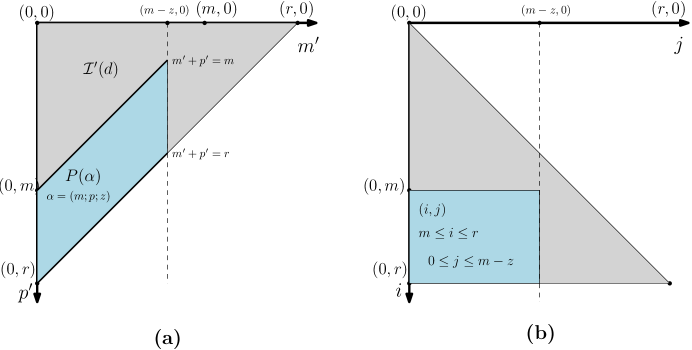
Figure 2: The transformation from $(m^{\prime},p^{\prime})$ to $(j,i)$ described in the text. From Definition 6, if $(m^{\prime},p^{\prime},z^{\prime})\in\mathcal{I}^{\prime}(d)$ then $z^{\prime}=d-2m^{\prime}-2p^{\prime}$ is uniquely determined by ($m^{\prime},p^{\prime}).$ In (a), the right triangle bounded by vertices $(0,0)$, $(0,r)$ and $(r,0)$ with $r=\lfloor d/2\rfloor$ is the location of all $(p^{\prime},m^{\prime})$ pairs such that $(m^{\prime},p^{\prime},z^{\prime})\in\mathcal{I}^{\prime}(d)$. The blue shaded parallelogram is the location of all $(p^{\prime},m^{\prime})$ pairs such that $(m^{\prime},p^{\prime},z^{\prime})\in P(\alpha)$ for some $\alpha=(m,p,z)\in\mathcal{I}(d).$ (b) illustrates the transformation $(j,i)=(m^{\prime},m^{\prime}+p^{\prime}).$ Note how the blue parallelogram becomes a rectangle, permitting the use of a 2D RRMQ query.

$$j=m^{\prime}\quad\mbox{and}\quad i=m^{\prime}+p^{\prime}.$$

Trivially $j\leq i.$ Furthermore,

$$(m^{\prime};p^{\prime};z^{\prime})\in{\cal I}^{\prime}(d)\quad\Rightarrow\quad d=2m^{\prime}+2p^{\prime}+z^{\prime}=2i+z^{\prime}$$

which in turn implies

$$2i\leq d\quad\mbox{and}\quad z^{\prime}=d-2i.$$

Set $r=\lfloor d/2\rfloor.$ Then

$$(m^{\prime};p^{\prime};z^{\prime})\in{\cal I}^{\prime}(d)\quad\Rightarrow\quad 0\leq j\leq i\leq r\quad\mbox{and}\quad(m^{\prime};p^{\prime};z^{\prime})=(j;i-j;d-2i).$$ (11)

Furthermore, working backwards,

$$0\leq j\leq i\leq r\quad\mbox{and}\quad(i-j;d-2i)\not=(0,0)\quad\Rightarrow\quad(j;i-j;d-2i)\in{\cal I}^{\prime}(d).$$ (12)

where the second condition comes from the fact that $(m^{\prime},p,z^{\prime})\not\in\mathcal{I}^{\prime}(d)$ if $(p^{\prime},z^{\prime})=(0,0)$.

The preceding discussion motivates defining the $(r+1)\times(r+1)$ matrix (indices of $i$ and $j$ start at $0$)

$$\small M^{(d)}_{i,j}\triangleq\begin{cases}\infty&\mbox{if $i>j$}\\ \infty&\mbox{if $i=j=\frac{d}{2}$}\\ \mathrm{OPT}_{0}(j;i-j;d-2i)+CW_{j-(d-2i),j}&\mbox{Otherwise}.\end{cases}$$

Since all the values referenced are already known, this matrix can be built in $O(r^{2})=O(n^{2})$ time.

Then, if $\alpha\in{\cal I}(d),$ from Corollary 1,

$$\mathrm{OPT}_{0}(\alpha) = \min_{\alpha^{\prime}=(m^{\prime};p^{\prime},z^{\prime})\in P(\alpha)}\{\mathrm{OPT}_{0}(\alpha^{\prime})+CW_{m^{\prime}-z^{\prime},m^{\prime}}\}$$

$$= \min\{M^{(d)}_{i,j}\,:\,i=m^{\prime}+p^{\prime}\geq m\mbox{ and }j=m^{\prime}\leq m-z\}$$

$$= RMQ\left(M^{(d)}_{i,j}:m,r,0,m-z\right)$$

$$= RRMQ\left(M^{(d)}_{i,j}:m,m-z\right)$$

Note that the RRMQ query result also provides the indices of the minimizing entry, which provides the corresponding $\mathrm{Pred}_{0}(\alpha)$ value as well.

Lemma 2 permits calculating all the $O(r^{2})$ $RRMQ\left(M^{(d)}_{i,j}:a,b\right)$ values in $O(r^{2})=O(n^{2})$ time. Thus, all of the $\mathrm{OPT}_{0}(\alpha)$ for $\alpha\in{\cal I}(d)$ (and their corresponding $\mathrm{Pred}_{0}(\alpha)$ values) can be calculated in $O(n^{2})$ total time. Doing this for all $O(n)$ values of $d>\bar{d}_{0}$ in increasing order, yields the required $O(n^{3})$ time algorithm for filling in the $\mathrm{OPT}_{0}$ matrix.

We next describe the more complicated algorithm for the $\mathrm{OPT}_{1}$ case.

Assume that $\mathrm{OPT}_{1}(\alpha)$ is already known for all $\alpha\in{\cal I}^{\prime}(d)$, $d^{\prime}<d.$ If $\alpha=(m;p;q)\in{\cal I}(d)$ then, similar to the $\mathrm{OPT}_{0}$ case,

$$\mathrm{OPT}_{1}(\alpha) = \min_{\alpha^{\prime}=(m^{\prime};p^{\prime},z^{\prime})\in P(\alpha)}\{\mathrm{OPT}_{1}(\alpha^{\prime})-CW_{m^{\prime},m-z}\}$$

where all the $\mathrm{OPT}_{1}(\alpha^{\prime})$ for $\alpha^{\prime}\in P(\alpha)$ are already known.

Following the approach in the $\mathrm{OPT}_{0}$ algorithm, for fixed $d,$ we would like to arrange the $O(n^{2})$ values $\left(\mathrm{OPT}_{1}(\alpha^{\prime})-CW_{m^{\prime},m-z}\right)$ for $\alpha^{\prime}=(m^{\prime};p^{\prime};z^{\prime})\in{\cal I}^{\prime}(d)$, appropriately in an array so that each $\mathrm{OPT}_{1}(\alpha)$ entry could be resolved using one 2D RMQ query. The difficulty is that the values of the array entries depend upon both $\alpha$ and $\alpha^{\prime}$. More specifically, the $CW_{m^{\prime},m-z}$ term would have to be reprocessed for each $(m,z)$ pair. Thus, no fixed $M_{i,j}$ array, independent of $(m,z)$, could be defined.

Instead, we utilize a relationship between different queries. More specifically, let $\alpha=(m;p;z)\in{\cal I}(d)$. From Equation (7), $z\leq m-m^{\prime}\leq m.$ If $z=m,$ then $m^{\prime}=0$ so $W_{m^{\prime},m-z}=W_{0,0}=0$ and

$$\mathrm{OPT}_{1}(\alpha) = \min_{\alpha^{\prime}=(m^{\prime};p^{\prime},z^{\prime})\in P(\alpha)}\{\mathrm{OPT}_{1}(\alpha^{\prime})-CW_{m^{\prime},m-z}\}$$

$$= \min_{\alpha^{\prime}=(m^{\prime};p^{\prime},z^{\prime})\in P(\alpha)}\{\mathrm{OPT}_{1}(\alpha^{\prime})\}.$$

If $z<m$ then, splitting into the cases $m^{\prime}=m-z$ and $m^{\prime}\leq m-z-1$ yields,

$$\mathrm{OPT}_{1}(\alpha)=\min(A,B)$$

where

$$A \triangleq \min_{\begin{subarray}{c}\alpha^{\prime}=(m^{\prime};p^{\prime},z^{\prime})\in P(\alpha)\\ m^{\prime}=m-z\end{subarray}}\{\mathrm{OPT}_{1}(\alpha^{\prime})-CW_{m^{\prime},m-z}\},$$

$$B \triangleq \min_{\begin{subarray}{c}\alpha^{\prime}=(m^{\prime};p^{\prime},z^{\prime})\in P(\alpha)\\ m^{\prime}\leq m-z-1\end{subarray}}\{\mathrm{OPT}_{1}(\alpha^{\prime})-CW_{m^{\prime},m-z}\}.$$

First note that if $m^{\prime}=m-z$, then $W_{m^{\prime},m-z}=0$ so

$$A = \min_{\begin{subarray}{c}\alpha^{\prime}=(m^{\prime};p^{\prime},z^{\prime})\in{\cal I}^{\prime}(d)\\ m^{\prime}+p^{\prime}\geq m\\ m^{\prime}=m-z\end{subarray}}\{\mathrm{OPT}_{1}(\alpha^{\prime})\}.$$

Next note that, from Corollary 1,

$$P((m;p;z))\cap \{(m^{\prime};p^{\prime};z^{\prime})\,:\,m^{\prime}\leq m-z-1\}$$

$$= \Bigl{\{}(m^{\prime};p^{\prime};z^{\prime})\in{\cal I}^{\prime}(2m+p))\,:\,m^{\prime}+p^{\prime}\geq m\mbox{ and }m^{\prime}\leq m-z-1\Bigr{\}}$$

$$= P((m;p;z+1))$$

and from Definition 3

$$W_{m^{\prime},m-z}=p_{m-z}+W_{m^{\prime},m-(z+1)}.$$

Thus

$$B = -Cp_{m-z}+\min_{\alpha^{\prime}=(m^{\prime};p^{\prime},z^{\prime})\in P((m;p;z+1))}\bigl{\{}\mathrm{OPT}_{1}(\alpha^{\prime})-CW_{m^{\prime},m-(z+1)}\bigr{\}}$$

$$= \mathrm{OPT}_{1}(m;p;z+1)-Cp_{m-z}$$

Again use the same transformation $j=m^{\prime}$ and $i=m^{\prime}+p^{\prime}$ so that Equations 11 and 12 apply. Set $r=\lfloor d/2\rfloor$, define the $(r+1)\times(r+1)$ array

$$M^{[d]}_{i,j}\triangleq\begin{cases}\infty&\mbox{if $i<j$}\\ \infty&\mbox{if $i=j=\frac{d}{2}$}\\ \mathrm{OPT}_{1}(j;i-j;d-2i)&\mbox{Otherwise}.\end{cases}$$

Next, use Lemma 2 to calculate all the $O(r^{2})$ $RCQ\left(M^{(d)}_{i,j}:a,b\right)$ values in $O(r^{2})=O(n^{2})$ time.

Let $\alpha=(m;p;z)\in{\cal I}(d)$. Then, from the discussion above,

• $$\mathrm{OPT}_{1}(\alpha) = \min_{\begin{subarray}{c}\alpha^{\prime}=(m^{\prime};p^{\prime},z^{\prime})\in{\cal I}^{\prime}(d)\\ m^{\prime}+p^{\prime}\geq m\\ m^{\prime}=0\end{subarray}}\{\mathrm{OPT}^{1}(\alpha^{\prime})\}$$

  $$= \min\left\{M^{[d]}_{i,j}\,:\,i\geq m\mbox{ and }j=0\right\}$$

  $$= RMQ\left(M^{[d]}_{i,j}:m,r,0,0\right)$$

  $$= RCQ\left(M^{[d]}_{i,j}:m,0\right)$$

  which is already known.

• $$A = \min_{\begin{subarray}{c}\alpha^{\prime}=(m^{\prime};p^{\prime},z^{\prime})\in{\cal I}^{\prime}(d)\\ m^{\prime}+p^{\prime}\geq m\\ m^{\prime}=m-z\end{subarray}}\{\mathrm{OPT}_{1}(\alpha^{\prime})\}$$

  $$= \min\left\{M^{[d]}_{i,j}\,:\,i\geq m\mbox{ and }j=m-z\right\}$$

  $$= RMQ\left(M^{[d]}_{i,j}:m,r,m-z,m-z\right)$$

  $$= RCQ\left(M^{[d]}_{i,j}:m,m-z\right).$$

  Thus, for $\alpha=(m;p;z)$ with $z<m$,

  $$\mathrm{OPT}_{1}(\alpha) = \min(A,B)$$

  $$= \min\Bigl{(}RCQ\left(M^{[d]}_{i,j}:m,m-z\right),\,\mathrm{OPT}_{1}(m;p;z+1)-Cp_{m-z}\Bigr{)}$$

  which, since $RCQ\left(M^{[d]}_{i,j}:m,m-z\right)$ is already known, can be calculated in $O(1)$ time if $\mathrm{OPT}_{1}(m;p;z+1)$ had already been calculated. The associated $\mathrm{Pred}_{1}(\alpha)$ can be found appropriately.

This permits calculating $\mathrm{OPT}_{1}(\alpha)$ and (and their corresponding $\mathrm{Pred}_{1}(\alpha)$ values) for all $\alpha=(m;p;z)\in{\cal I}(d)$ in a total of $O(n^{2})$ time as follows:

1. First spend $O(n^{2})$ time calculating all the $RCQ\left(M^{(d)}_{i,j}:a,b\right)$ values.

2. For each of the $O(n)$ possible fixed pairs $m,p$ satisfying $2m+p=d$

   1. Set $\mathrm{OPT}_{1}(m;p;m)=RRMQ\left(M^{[d]}_{i,j}:m,0\right)$.

   2. Then, for $z=m-1,m-2,\ldots,$ calculate $\mathrm{OPT}_{1}(m;p;z)$ in $(1)$ time from $\mathrm{OPT}_{1}(m;p;z+1)$ using Equation (If $z<m$,).

Since this is $O(n^{2})$ time for fixed $d,$ doing this for all $O(n)$ values of $d>\bar{d}_{1}$ in increasing order yields the required $O(n^{3})$ time algorithm for filling in the $\mathrm{OPT}_{1}$ matrix.

4 A Quick Introdution to AIFV-$2$ codes

Note: This introduction is copied with some small modifications, from [8].

Let $X$ be a memoryless source over a finite alphabet $\mathcal{X}$ of size $n$. $\forall a_{i}\in\mathcal{X}$, let $p_{i}=P_{X}(a_{i})$ denote the probability of $a_{i}$ ocurring. Without loss of generality we assume that

$$p_{1}\geq p_{2}\geq\cdots\geq p_{n}>0\text{ and }\sum_{i=1}^{n}p_{i}=1.$$

A codeword $c$ of a binary AIFV code is a string in $\{0,1\}^{*}.$ $|c|$ will denote the length of codeword $c$.

Figure 3: A binary AIFV-$2$ code for $\mathcal{X}=\{a,b,c,d\}$ with associated probabilities. The encoding of ${\bf b}d{\bf b}c{\bf a}a$ is ${\bf Y}={\bf 10}1100{\bf 10}11{\bf 01}0.$ Note that $d,c$ and the first $a$ were encoded using $T_{1}$ while the other letters were encoded using $T_{0}.$ This code has cost $\approx 1.72$ which is better than the optimal Huffman code for the same source which has $L(\rm{Huffman_{\mathcal{X}}})=1.75$

We now briefly describe the structure of Binary AIFV-$2$ codes using the terminology of [9]. See [9] for more details and Figure 3 for an example.

Codes are represented via binary trees with left edges labelled by “$0$” and right edges by “$1$”. A Binary AIFV-$2$ code is a pair of binary code trees, $T_{0},T_{1}$ satisfying:

• Complete internal nodes in $T_{0}$ and $T_{1}$ have both left and right children.

• Incomplete internal nodes (with the unique exception of the left child of the root of $T_{1}$) have only a “$0$” (left) child.
  Incomplete internal nodes are labelled as either master nodes or slave nodes.

• A master node must be an incomplete node with an incomplete child
  The child of a master node is a slave node.
  This implies that a master node is connected to its unique grandchild via “$00$” with the intermediate node being a slave node.

• Each source symbol is assigned to one node in $T_{0}$ and one node in $T_{1}$.
  The nodes to which they are assigned are either leaves or master nodes.
  Symbols are not assigned to complete internal nodes or slave nodes.

• The root of $T_{1}$ is complete and its “$0$” child is a slave node.
  The root of $T_{1}$ has no “$00$” grandchild.

Let $c_{s}(a),s\in\{0,1\}$ denote the codeword of $a\in\mathcal{X}$ encoded by $T_{s}$. The encoding procedure for a sequence $x_{1},x_{2}\ldots$ of source symbols works as follows.
0. Set $s_{1}=0$ and $j=1.$
1. Encode $x_{j}$ as $c_{s_{j}}(x_{j}).$
2. If $c_{s_{j}}(x_{j})$ is a leaf in $T_{s_{j}}$, then set $s_{j+1}=0$
          else set $s_{j+1}=1$  % this occurs when $c_{s_{j}}(x_{j})$ is a master node in $T_{s_{j}}$
3. Set $j=j+1$ and Goto 1.

Note that a symbol is encoded using $T_{0}$ if and only if its predecessor was encoded using a leaf node and it is encoded using $T_{1}$ if and only if its predecessor was encoded using a master node. The decoding procedure is a straightforward reversal of the encoding procedure. Details are provided in [14] and [10]. The important observation is that identifying the end of a codeword might first require reading an extra two bits past its ending, resulting in a two bit delay, so decoding is not instantaneous.

Following [14], we can now derive the average codeword length of a binary AIFV-$2$ code defined by trees $T_{0},T_{1}$. The average codeword length $L(T_{s})$ of $T_{s}$, $s\in\{0,1\},$ is

$$L(T_{s})=\sum_{i=1}^{n}|c_{s}(a_{i})|p_{i}.$$

If the current symbol $x_{j}$ is encoded by a leaf (resp. a master node) of $T_{s_{j}}$, then the next symbol $x_{j+1}$ is encoded by $T_{0}$ (resp. $T_{1}$). This process can be modelled as a two-state Markov chain with the state being the current encoding tree. Denote the transition probabilities for switching from code tree $T_{s}$ to $T_{s^{\prime}}$ by $q_{s^{\prime}}(T_{s})$. Then, from the definition of the code trees and the encoding/decoding protocols:

$$q_{0}(T_{s})=\sum_{a\in\mathcal{L}_{T_{s}}}P_{X}(a)\quad\mbox{and}\quad q_{1}(T_{s})=\sum_{a\in\mathcal{M}_{T_{s}}}P_{X}(a)$$

where $\mathcal{L}_{T_{s}}$ (resp. $\mathcal{M}_{T_{s}})$ denotes the set of source symbols $a\in\mathcal{X}$ that are assigned to a leaf node (resp. a master node) in $T_{s}$.

Given binary AIFV-$2$ code $T_{0},T_{1},$ as the number of symbols being encoded approaches infinity, the stationary probability of using code tree $T_{s}$ can then be calculated to be

$$P(s|T_{0},T_{1})=\frac{q_{s}(T_{\hat{s}})}{q_{1}(T_{0})+q_{0}(T_{1})}$$ (14)

where $\hat{s}\in\{0,1\},s\neq\hat{s}$.

The average (asymptotically) codeword length (as the number of characters encoded goes to infinity) of a binary AIFV-$2$ code is then

$$L_{AIFV}(T_{0},T_{1})=P(0|T_{0},T_{1})L(T_{0})+P(1|T_{0},T_{1})L(T_{1})$$ (15)

Algorithm 1 Iterative algorithm to construct an optimal binary AIFV-$2$ code [15, 10]

1:$m\leftarrow 0;$  $C^{(0)}=2-\log_{2}(3)$

2:repeat

3:     $m\leftarrow m+1$

4:     $T_{0}^{(m)}=\text{argmin}_{T_{0}\in\mathcal{T}_{0}(n)}\{L(T_{0})+C^{(m-1)}q_{1}(T_{0})\}$

5:     $T_{1}^{(m)}=\text{argmin}_{T_{1}\in\mathcal{T}_{1}(n)}\{L(T_{1})-C^{(m-1)}q_{0}(T_{1})\}$

6:     Update

$$C^{(m)}=\frac{L\left(T_{1}^{(m)}\right)-L\left(T_{0}^{(m)}\right)}{q_{1}\left(T_{0}^{(m)}\right)+q_{0}\left(T_{1}^{(m)}\right)}$$

7:until $C^{(m)}=C^{(m-1)}$

8:// Set $C^{*}=C^{(m)}.$ Optimal binary AIFV-$2$ code is $T_{0}^{(m)}$, $T_{1}^{(m)}$

[14, 15] showed that the binary AIFV-$2$ code $T_{0},T_{1}$ minimizing Equation 15 can be obtained by Algorithm 1, in which $\mathcal{T}_{0}(n)$ (resp. $\mathcal{T}_{1}(n)$) is the set of all possible $T_{0}$ (resp. $T_{1}$) coding trees. It implemented the minimization (over all coding trees) in lines 4 and 5 as an ILP. In a later paper [10], the authors replaced this ILP with a $O(n^{5})$ time and $O(n^{3})$ space DP that modified a top-down tree-building DP from [6, 4].

[10, 15] proved algebraically that Algorithm 1 would terminate after a finite number of steps and that the resulting tree pair $T_{0}^{(m)},$ $T_{1}^{(m)}$ is an optimal Binary AIFV-$2$ code. They were unable, though, to provide any bounds on the number of steps needed for termination. [7] then gave two new iterative algorithms that provably terminated in $O(b)$ iterations, where $b$ is the maximum number of bits required to store any of the probabilities $p_{i}$ (so these were weakly polynomial algorithms). More formally, let $o_{i},b_{i}$ be such that $p_{i}=o_{i}2^{-b_{i}}$ where $o_{i}<2^{b_{i}}$ is an odd positive integer. Then $b=\max_{i}b_{i}.$

Each iteration step of [7]’s algorithm ran $O(1)$ of the DPs from [10] so its full algorithm for constructing optimal AIFV-$2$ codes ran in $O(n^{5}b)$ time. The results of this paper replace the $O(n^{5})$-time DPs with $O(n^{3})$-time DPs, leading to $O(n^{3}b)$-time algorithms for constructing optimal AIFV-$2$ codes.

We conclude this section by noting that the correctness of the DPs defined in both [10] and the next section assume that $0\leq C^{(i)}\leq 1$. The need for this assumption was implicit in [10] and is made explicit in Lemma 5 in the next section. The validity of this assumption was proven in [8].

5 Deriving the DP

Each iteration step in both [10] and [7] requires finding trees that satisfy

$$T_{0}(C)\triangleq\text{argmin}_{T_{0}\in\mathcal{T}_{0}(n)}\left\{\mathrm{Cost}_{0}(T_{0}:C)\right\},$$ (16)

$$T_{1}(C)\triangleq\text{argmin}_{T_{1}\in\mathcal{T}_{1}(n)}\left\{\mathrm{Cost}_{1}(T_{1}:C)\right\},$$ (17)

where

$$\mathrm{Cost}_{0}(T:C)\triangleq L(T)+Cq_{1}(T),$$ (18)

$$\mathrm{Cost}_{1}(T:C)\triangleq L(T)-Cq_{0}(T).$$ (19)

Since $C$ will be fixed at any iteration stage, we simplify our notation by assuming $C$ fixed and writing $\mathrm{Cost}_{0}(T)$ and $\mathrm{Cost}_{1}(T)$ to denote Equations 18 and 19.

Definition 7.

Let $T$ be a binary AIFV coding tree. Define

$$\forall a_{i}\in\mathcal{X},\quad\begin{array}[]{ccl}c_{T}(a_{i})&\triangleq&\mbox{codeword in $T$ associated with $a_{i}$},\\ d_{T}(i)&\triangleq&|c_{T}(a_{i})|.\end{array}$$

By the natural correspondence, $d_{T}(i)$ is the depth of the node in $T$ associated with $a_{i}$ so $L(T)=\sum_{i=1}^{n}d_{T}(i)p_{i}.$ Further define

$$\forall a_{i}\in\mathcal{X},\quad m_{T}(i)\triangleq\begin{cases}1&\mbox{if $c_{T}(a_{i})$ is a master node in $T$},\\ 0&\mbox{if $c_{T}(a_{i})$ is a leaf in $T$,}\end{cases},\quad\ell_{T}(i)\triangleq\begin{cases}0&\mbox{if $m_{T}(i)=1$}.\\ 1&\mbox{if $m_{T}(i)=0$}.\end{cases}$$

$m_{T}(i)$ and $\ell_{T}(i)$ are indicator functions as to whether $a_{i}$ is encoded by a master node or a leaf in $T,$ so, $\forall i,$ $m_{T}(i)+\ell_{T}(i)=1.$

Note that using this new notation

$$\mathrm{Cost}_{0}(T) = \sum_{i=1}^{n}d_{T}(i)p_{i}+C\sum_{i=1}^{n}m_{T}(i)p_{i},$$

$$\mathrm{Cost}_{1}(T) = \sum_{i=1}^{n}d_{T}(i)p_{i}-C\sum_{i=1}^{n}\ell_{T}(i)p_{i}.$$

We now show that $0\leq C\leq 1$ implies that $T_{0}(C)$ and $T_{1}(C)$ can be assumed to possess a nice ordered structure.

Lemma 5.

Let $0\leq C\leq 1$. Then, if $s=0$ (resp. $s=1$) there exists a tree $T_{0}(C)\in\mathcal{T}_{0}(n)$ (resp. $T_{1}(C)\in\mathcal{T}_{1}(n)$) satisfying Equation 16 (resp. Equation 17) that, for all $i<j$, satisfies the following two properties:

1. $d_{T_{s}}(i)\leq d_{T_{s}}(j).$

2. If $d_{T_{s}}(i)=d_{T_{s}}(j)$ and $m_{T_{s}}(i)=1$ then $m_{T_{s}}(j)=1$.

Proof.

We say that $T_{1}=T_{1}(C)$ (resp $T_{2}=T_{2}(C)$) is a minimum cost tree (for $s$) if it satisfies Equation (16) (resp. (17)).

The proof follows from swapping arguments. “Swapping” $i$ and $j$ means assigning the old codeword $c_{T_{s}}(a_{i})$ to $a_{j}$ and vice-versa. Let $T^{\prime}_{s}$ be the tree resulting from swapping $i$ and $j$.

The following observation is a straightforward calculation:

$$\mathrm{Cost}_{s}(T^{\prime}_{s})=\mathrm{Cost}_{s}(T_{s})-\left(d_{T_{s}}(i)-d_{T_{s}}(j)\right)(p_{i}-p_{j})+\delta(i,j)$$

where

$$\delta(i,j)\triangleq\begin{cases}0&\mbox{ if $m_{T_{s}}(i)=m_{T_{s}}(j)$},\\ -C(p_{i}-p_{j})&\mbox{ if $m_{T_{s}}(i)=1$, and $\ell_{T_{s}}(j)=1$},\\ C(p_{i}-p_{j})&\mbox{ if $\ell_{T_{s}}(i)=1$, and $m_{T_{s}}(j)=1$}.\end{cases}$$

We say that $(i,j)$ is an inversion for $T_{s}$ if $i<j$ and $d_{T_{s}}(i)>d_{T_{s}}(j)$.

The calculations above and the fact that $0\leq C\leq 1$, immediately imply that if $(i,j)$ is an inversion for $T_{s}$ then

$$\mathrm{Cost}_{s}(T^{\prime}_{s})\leq\mathrm{Cost}_{s}(T_{s}).$$

Now let $T_{s}$ be a minimum cost tree for $s$ that has the minimum number of inversions among all such trees. If no inversion exists, then $T_{s}$ satisfies (P1). Otherwise, let $(i,j)$ be the inversion that minimizes $j-i$. Swapping $i$ and $j$ decreases the number of inversions by $1$ while not increasing the cost of the tree, contradicting the definition of $T_{s}$. We may therefore assume that $T_{s}$ contains no inversion and satisfies (P1).

Now say that $(i,j)$ is an $m\ell$-inversion in $T_{s}$ if $i<j$, $d_{T_{s}}(i)=d_{T_{s}}(j)$, $m_{T_{s}}(i)=1$ and $\ell_{T_{s}}(j)=1$. Let $T_{s}$ be a minimum cost tree for $s$ that satisfies (P1) and has the fewest number of $m\ell$-inversions. If no $m\ell$-inversion exists, then $T_{s}$ also satisfies (P2) so the lemma is correct. Otherwise let $(i,j)$ be an $m\ell$-inversion that minimizes $j-i.$ Let $T^{\prime}_{s}$ be the tree that results by swapping $i$ and $j.$ Then $T^{\prime}_{s}$ will still satisfy (P1) but the numbers of inversions will decrease by $1$ while

$$\mathrm{Cost}_{s}(T^{\prime}_{s})=\mathrm{Cost}_{s}(T_{s})-C(p_{i}-p_{j})\leq\mathrm{Cost}_{s}(T_{s}).$$

This contradicts the definition of $T_{s}.$ We may therefore assume $T_{s}$ contains no inversions and satisfies both (P1) and (P2). ∎

The consequences of Lemma 5 can be seen in Figure 4. The Lemma implies that the optimization in Equation 16 (resp. Equation 17) can be restricted to trees that satisfy Properties (P1) and (P2). In particular, the indices of codewords on a level are smaller than the indices of codewords on deeper levels. Also, on any given level, the indices of the leaves are smaller than the indices of the master nodes. We therefore henceforth assume that all trees in $\mathcal{T}_{0}(n),$ and $\mathcal{T}_{1}(n)$ satisfy these properties.

Definition 8 (Partial Trees and Truncation).

See Figure 5.

• A partial binary AIFV code tree (partial tree for short) $T$ is one that satisfies all of the conditions of a binary AIFV code tree and properties (P1), (P2) except that it contains $m\leq n$ codewords. By (P1), the $m\leq n$ codewords it contains are $c_{T}(a_{1}),\ldots,c_{T}(a_{m}).$

• For $s\in\{0,1\}$, let $\bar{\mathcal{T}}_{s}(n)$ denote the set of partial trees that satisfy the conditions of $T_{s}$ trees.

  For notational convenience, also set

  $$\mathcal{T}(n)\triangleq\mathcal{T}_{0}(n)\cup\mathcal{T}_{1}(n)\quad\mbox{and}\quad\bar{\mathcal{T}}(n)\triangleq\bar{\mathcal{T}}_{0}(n)\cup\bar{\mathcal{T}}_{1}(n).$$

• $T\in\bar{\mathcal{T}}(n)$ is $i$-level if $0pt(T)\leq i+1.$ Set

  $$\bar{\mathcal{T}}_{s}(i:n)\triangleq\left\{T_{s}\in\bar{\mathcal{T}}_{s}(n)\,:\,T_{s}\mbox{ is $i$-level}\right\}\quad\mbox{and}\quad\bar{\mathcal{T}}(i:n)\triangleq\bar{\mathcal{T}}_{0}(i:n)\cup\bar{\mathcal{T}}_{1}(i:n).$$

• Let $T\in\mathcal{T}(n)$. The $i$-level truncation of $T,$ denoted by $\mathrm{Trunc}^{(i)}(T)$, is the partial tree that remains after removing all nodes at depth $j>i+1$ from $T.$

Note: $\forall T\in{\mathcal{T}}(n),$ $\mathrm{Trunc}^{(i)}(T)\in\bar{\mathcal{T}}(i:n).$

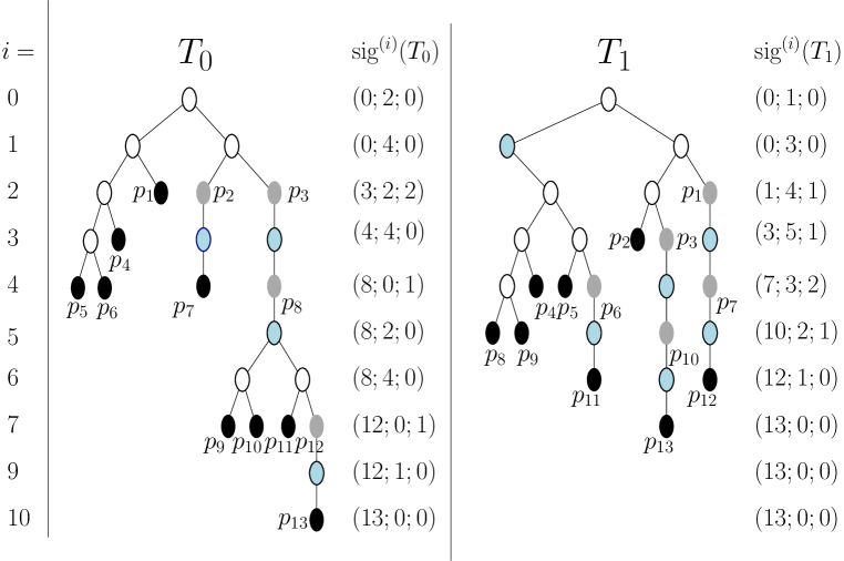
Figure 4: Black nodes are leaves, gray nodes master nodes and blue ones slave nodes. Note that on every level, the indices of the leaves are smaller than the indices of the master nodes. Also note that in all cases, if $\mathrm{sig}^{(i)}(T_{s})=\left(m^{\prime};p^{\prime},z^{\prime}\right)$ and $\mathrm{sig}^{(i+1)}(T_{s})=\left(m;p,z\right)$ then $2m^{\prime}+2p^{\prime}+z^{\prime}=2m+p,$ $m^{\prime}+p^{\prime}\geq m$ and $m^{\prime}\leq m-z,$ as required by Lemma 3.

Definition 9 (Signatures and Costs).

See Figures 4 and 5.

(a) $i-$level Signatures: The $i-$level signature of $T$ is the ordered triple

$$\mathrm{sig}^{(i)}(T)\triangleq(m;p;z)$$

where

$$m \triangleq |\{j\,:\,d_{T}(j)\leq i\}|=\mbox{\# of codewords on or above level $i$ of $T$},$$

$$p \triangleq \mbox{\# of non-slave nodes on level $i+1$ of $T$},$$

$$z \triangleq |\{j\,:\,d_{T}(j)=i\mbox{ and }m_{T}(j)=1\}|=\mbox{\# of master nodes on level $i$ of $T$}.$$

Note that

$$\mathrm{sig}^{(i)}(T)=\mathrm{sig}^{(i)}\left(\mathrm{Trunc}^{(i)}(T)\right).$$

(b) $i$-level Costs:

Let $\mathrm{sig}^{(i)}(T)=(m;p;z).$ The $i$-level costs of $T$ are

$$\mathrm{Cost}_{0}^{(i)}(T)\triangleq iW^{\prime}_{m}+\sum_{i=1}^{m}d_{T}(i)p_{i}+C\sum_{i=1}^{m-z}m_{T}(i)p_{i}.$$

and

$$\mathrm{Cost}_{1}^{(i)}(T)\triangleq iW^{\prime}_{m}+\sum_{i=1}^{m}d_{T}(i)p_{i}-C\sum_{i=1}^{m}\ell_{T}(i)p_{i}.$$

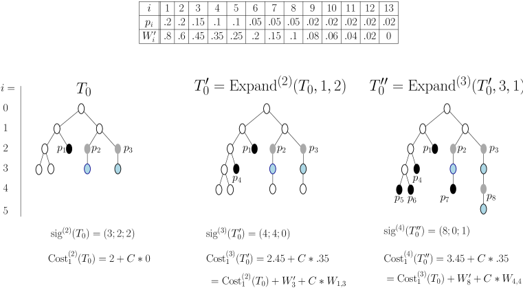
Figure 5: Illustrations of the $\mathrm{Trunc}$ and $\mathrm{Expand}$ operations and Lemma 9. The $p_{i}$, $i=1,\ldots,13,$ are given in the table above the trees. As examples of the $\mathrm{Trunc}$ operation note that $\mathrm{Trunc}^{(2)}(T^{\prime\prime}_{0})=\mathrm{Trunc}^{(2)}(T^{\prime}_{0})=T_{0}$ and $\mathrm{Trunc}^{(3)}(T^{\prime\prime}_{0})=T^{\prime}_{0}.$

Suppose $T_{s}\in\bar{\mathcal{T}}_{s}(n),$ with $0pt(T)=d.$ An interesting peculiarity of this definition is that $T$ is an $i$ level tree for all $i\geq d-1$ and it is quite possible that

$$\mathrm{Cost}_{0}^{(d-1)}(T_{0})<\mathrm{Cost}_{0}^{(d)}(T_{0})<\mathrm{Cost}_{0}^{(d+1)}(T_{0})<\cdots$$

for some indeterminate length chain. The important observation though, is that $\mathrm{Cost}_{s}^{(i)}(T)$ collapses to $\mathrm{Cost}_{s}(T)$ for the interesting cases.

Lemma 6.

• Let $T_{s}\in{\mathcal{T}}_{s}(n),$ with $0pt(T_{s})=d.$
  Then $\mathrm{sig}^{(d)}(T_{s})=(n;0;0)$ and $\mathrm{Cost}_{s}^{(d)}(T_{s})=\mathrm{Cost}_{s}(T_{s}).$

• Let $T_{s}\in\bar{\mathcal{T}}_{s}(n)$ be an $i$-level tree with $\mathrm{sig}^{(i)}(T_{s})=(n;0;0)$.
  Then $T_{s}\in{\mathcal{T}}_{s}(n)$ with $depth(T_{s})=i$.

Proof.

(a) By definition, $T_{s}$ is a $d$-level tree with no nodes on level $d+1.$

Let $(m,p,z)=\mathrm{sig}^{(d)}(T_{s})$. Since $T_{s}$ contains $n$ codewords, $m=n.$ $T_{s}$ contains no nodes on level $d+1$, so $p=0.$ Furthermore, it contains no slave nodes on level $d+1$ so it contains no master nodes on level $d,$ i.e., $z=0.$

Since $W^{\prime}_{n}=0$,

$$\mathrm{Cost}_{0}^{(d)}(T_{0})=dW^{\prime}_{n}+\sum_{i=1}^{n}d_{T}(i)p_{i}+C\sum_{i=1}^{n}m_{T}(i)p_{i}=\mathrm{Cost}_{0}(T_{0}).$$

Similarly

$$\mathrm{Cost}_{1}^{(d)}(T_{1})=dW^{\prime}_{n}+\sum_{i=1}^{n}d_{T}(i)p_{i}-C\sum_{i=1}^{n}\ell_{T}(i)p_{i}=\mathrm{Cost}_{1}(T_{1}).$$

(b) $T_{s}$ contains no master nodes on level $i$ so it contains no slave nodes on level $i+1$. It also contains no non-slave nodes on level $i$. So it contains no nodes on level $i$ and $0pt(T_{s})=i.$ $T_{s}\in{\mathcal{T}}_{s}(n)$ by definition. ∎

The definitions and lemmas immediately imply

Corollary 2.

$$T_{s}(C)=\operatorname*{\arg\!\min}_{\begin{subarray}{c}T_{s}\in\bar{\mathcal{T}}(n)\\ \exists i\mbox{ s.t. }T_{s}\in\bar{\mathcal{T}}(i:n)\mbox{ and }\mathrm{sig}^{(i)}(T_{s})=(n;0;0)\end{subarray}}\mathrm{Cost}^{(i)}_{s}(T_{s})$$ (20)

The next definition introduces the initial conditions for the dynamic programs.

Definition 10.

See Figure 6. Set

$$I_{0} = \{(0;2;0),\,(1;0,1)\},$$

$$I_{1} = \{(0;3;0),\,(1;1;0),\,(1;1;1)\}.$$

Note that if $(m;p;z)\in I_{0}$, there exists a unique $0$-level tree $T_{s}\in\bar{\mathcal{T}}_{0}(n)$ satisfying $\mathrm{sig}^{(0)}(T_{0})=(m;p;z).$

Similarly, if $(m;p;z)\in I_{1}$, there exists a unique $1$-level tree $T_{s}\in\bar{\mathcal{T}}_{1}(n)$ satisfying $\mathrm{sig}^{(1)}(T_{1})=(m;p;z).$

Let $T_{s}(m;p;z)$ denote this unique tree and $\bar{c}_{s}(m;p;z)=\mathrm{Cost}_{s}^{(s)}(T_{s}(m;p;z)).$

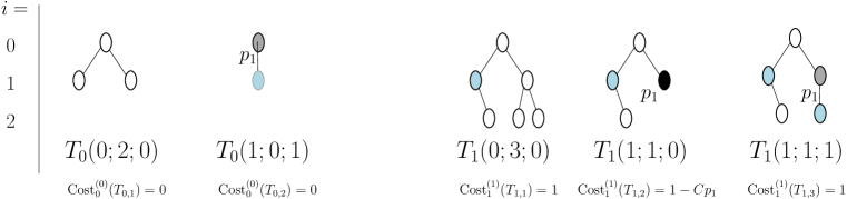
Figure 6: The initial trees introduced in Definition 10. Note that the definition of $T_{0}$ trees permit the root to be a master node or an internal node, while the definition of $T_{1}$ trees requires that the root be an internal node.

The following lemma is true by observation

Lemma 7.

Let $n>2$.
If $T_{0}\in\bar{\mathcal{T}}_{0}(n)$ with $0pt(T_{0})\geq 0$, then $\mathrm{sig}^{(0)}(T_{0})\in I_{0}.$
If $T_{1}\in\bar{\mathcal{T}}_{1}(n)$ with $0pt(T_{1})\geq 1$, then $\mathrm{sig}^{(1)}(T_{1})\in I_{1}.$

Note: The reason for starting with $\mathrm{sig}^{(1)}(T_{1})$ instead of $\mathrm{sig}^{(0)}(T_{1})$ is because the root of a $T_{1}$ tree is “unusual”, being a complete node with a slave child, the only time this combination can occur. By definition, $\mathrm{sig}^{(0)}(T_{1})=(0;1;0)$. This is misleading because it loses the information about the unusual slave node on level $1$. We therefore only start looking at signatures of $T_{1}$ trees from level $1$.

Definition 11.

See Figure 5. Let $T^{\prime}\in\bar{\mathcal{T}}(i:n)$ satisfy $\mathrm{sig}^{(i)}(T^{\prime})=(m^{\prime};p^{\prime};z^{\prime})$ and

$$e_{0},\,e_{1}\geq 0\quad\mbox{ \rm such that }\quad e_{0}+e_{1}\leq p^{\prime}.$$ (21)

Define the $(e_{0},e_{1})-$expansion of $T^{\prime}$ as the unique tree

$$T=\mathrm{Expand}^{(i)}(T^{\prime},e_{0},e_{1})$$

in which

• the first $i$-levels of $T$ are identical to those of $T^{\prime}.$

• $e_{0}$ of the $p^{\prime}$ non-slave nodes on level $i+1$ of $T^{\prime}$ are set as leaves associated with $a_{m^{\prime}+1}.\ldots,a_{m^{\prime}+e_{0}}.$

• $e_{1}$ non-slave nodes on level $i+1$ of $T^{\prime}$ are set as master nodes associated with $a_{m^{\prime}+e_{0}+1}.\ldots,a_{m^{\prime}+e_{0}+e_{1}}$ (with corresponding slave nodes created on level $i+2$).

• the remaining $p^{\prime}-e_{0}-e_{1}$ non-slave nodes on level $i+1$ of $T^{\prime}$ become complete internal nodes, creating $2(p^{\prime}-e_{0}-e_{1})$ non-slave nodes on level $i+2$. These are in addition to the $z^{\prime}$ non-slave children on level $i+2$ of the $z^{\prime}$ slave nodes on level $i+1.$

Note that this definition implies that $\mathrm{sig}^{(i+1)}(T)=(m;p;z)$ where

$$m = m^{\prime}+e_{0}+e_{1},$$ (22)

$$z = e_{1},$$ (23)

$$p = z^{\prime}+2(p^{\prime}-e_{0}-e_{1}).$$ (24)

Lemma 8.

• Let $T^{\prime}\in\bar{\mathcal{T}}(i:n)$. If $\mathrm{sig}^{(i)}(T^{\prime})=(m^{\prime};p^{\prime};z^{\prime})$ and $(e_{0},e_{1})$ satisfies Equation 21, then

  $$T^{\prime}=\mathrm{Expand}^{(i)}\left(T^{\prime\prime},\,e_{0},\,e_{1}\right)\in\bar{\mathcal{T}}(i+1:n).$$

• Let $T\in\bar{\mathcal{T}}(n).$ For $i\geq 0,$ set $\left(m^{(i)};p^{(i)};z^{(i)}\right)=\mathrm{sig}^{(i)}\left(\mathrm{Trunc}^{(i)}(T)\right).$ Then

  $$\mathrm{Trunc}^{(i+1)}(T)=\mathrm{Expand}^{(i)}\Bigl{(}\mathrm{Trunc}_{i}(T),\,e_{0},\,e_{1}\Bigr{)}$$

  where $e_{0}=m^{(i+1)}-m^{(i)}-z^{(i+1)}$ and $e_{1}=z^{(i+1)}.$

Proof.

(a) follows from the fact that Definition 1 maintains the validity of properties (P1) and (P2) of Lemma 5 and that $0pt(T^{\prime\prime})\leq i+2.$ (b) just follows directly from the definitions. ∎

Part (b) implies that any tree $T\in\bar{\mathcal{T}}(n)$ can be grown level by level via expansion operations.

Now recall from Definition 4 the definition of the signature set ${\cal S}_{n}$ and the operation $\rightarrow$.

Lemma 9.

Let $T^{\prime}\in\bar{\mathcal{T}}(i:n)$ with $\mathrm{sig}^{(i)}(T^{\prime})=\alpha^{\prime}=(m^{\prime};p^{\prime};z^{\prime})$.

• Let $(e_{0},e_{1})$ satisfy Equation 1.
  Let $T=\mathrm{Expand}^{(i)}(T^{\prime},e_{0},e_{1})$ and $\alpha=(m;p;z)=\mathrm{sig}^{(i+1)}(T).$

  Then $\alpha^{\prime}\rightarrow\alpha$.

• Let $\alpha=(m;p;z)$. If $\alpha^{\prime}\rightarrow\alpha$, let $e_{0},e_{1}$ be the unique values satisfying Equations (1)-(4) and set $T=\mathrm{Expand}^{(i)}(T^{\prime},e_{0},e_{1})$.

  Then $\alpha=\mathrm{sig}^{(i+1)}(T)$.

• If $T=\mathrm{Expand}^{(i)}(T^{\prime},e_{0},e_{1})$ with $\alpha=(m;p;z)=\mathrm{sig}^{(i+1)}(T)$, then

  $$\mathrm{Cost}_{0}^{(i+1)}(T)=\mathrm{Cost}_{0}^{(i)}(T^{\prime})+c_{0}(\alpha^{\prime},\,\alpha)$$

  $$\mathrm{Cost}_{1}^{(i+1)}(T)=\mathrm{Cost}_{1}^{(i)}(T^{\prime})+c_{1}(\alpha^{\prime},\,\alpha)$$

Proof.

(a) This follows directly from the definition of $T=\mathrm{Expand}^{(i)}(T^{\prime},e_{0},e_{1})$.

(b) From the definition of $\alpha^{\prime}\rightarrow\alpha$ there exist appropriate $e_{0},e_{1}$ satisfying Equations (1)-(4). Then $T=\mathrm{Expand}^{(i)}(T^{\prime},e_{0},e_{1})$ has $\mathrm{sig}^{(i+1)}(T)=(m;p;z).$

(c) From the definitions of signatures and expansions

$$\sum_{j=1}^{m^{\prime}}d_{T}(j)p_{j}=\sum_{j=1}^{m^{\prime}}d_{T^{\prime}}(j)p_{j}\quad\mbox{and}\quad\sum_{j=m^{\prime}+1}^{m}d_{T}(j)p_{j}=(i+1)\sum_{j=m^{\prime}+1}^{m}p_{j}=(i+1)W_{m^{\prime},m}.$$

Furthermore, from Lemma 5 (P1), (P2), the master nodes on level $i$ correspond to $a_{m^{\prime}-z^{\prime}+1},\ldots,a_{m^{\prime}}$. Thus (again also using the definition of expansion)

$$\sum_{j=1}^{m^{\prime}-z^{\prime}}m_{T}(j)p_{j}=\sum_{j=1}^{m^{\prime}-z^{\prime}}m_{T^{\prime}}(j)p_{j}\quad\mbox{and}\quad\sum_{j=m^{\prime}-z^{\prime}+1}^{m-z}m_{T}(j)p_{j}=\sum_{j=m^{\prime}-z^{\prime}+1}^{m-z}p_{j}=W_{m^{\prime}-z^{\prime},m^{\prime}}.$$

Then

$$\mathrm{Cost}_{0}^{(i+1)}(T) = (i+1)W^{\prime}_{m}+\sum_{j=1}^{m}d_{T}(j)p_{j}+C\sum_{j=1}^{m-z}m_{T}(j)p_{j}$$

$$= (i+1)W^{\prime}_{m}+(i+1)W_{m^{\prime},m}+\sum_{j=1}^{m^{\prime}}d_{T^{\prime}}(j)p_{j}$$

$$\hskip 57.81621pt+C\sum_{j=1}^{m^{\prime}-z^{\prime}}m_{T^{\prime}}(j)p_{j}+C\sum_{j=m^{\prime}-z^{\prime}+1}^{m-z}m_{T}(j)p_{j}$$

$$= (i+1)W^{\prime}_{m^{\prime}}+\sum_{j=1}^{m^{\prime}}d_{T^{\prime}}(j)p_{j}+C\sum_{j=1}^{m^{\prime}-z^{\prime}}m_{T^{\prime}}(j)p_{j}+C\sum_{j=m^{\prime}-z^{\prime}+1}^{m-z}m_{T}(j)p_{j}$$

$$= iW^{\prime}_{m^{\prime}}+\sum_{j=1}^{m^{\prime}}d_{T^{\prime}}(j)p_{j}+C\sum_{j=1}^{m^{\prime}-z^{\prime}}m_{T^{\prime}}(j)p_{j}+W^{\prime}_{m^{\prime}}+CW_{m^{\prime}-z^{\prime},m^{\prime}}$$

$$= \mathrm{Cost}_{0}^{(i)}(T^{\prime})+c_{0}(\alpha^{\prime},\,\alpha).$$

From Lemma 5 (P1), (P2), the leaves on level $i+1$ of $T$ correspond to $a_{m^{\prime}+1},\ldots,a_{m-z}$. Thus (again also using the definition of expansion)

$$\sum_{j=1}^{m^{\prime}}\ell_{T}(j)p_{j}=\sum_{j=1}^{m^{\prime}}\ell_{T^{\prime}}(j)p_{j}\quad\mbox{and}\quad\sum_{j=m^{\prime}+1}^{m^{\prime}}\ell_{T}(j)p_{j}=\sum_{j=m^{\prime}+1}^{m-z}p_{j}=W_{m^{\prime},m-z}.$$

Then

$$\mathrm{Cost}_{1}^{(i+1)}(T) = (i+1)W^{\prime}_{m}+\sum_{j=1}^{m}d_{T}(j)p_{j}-C\sum_{j=1}^{m}\ell_{T}(j)p_{j}$$

$$= (i+1)W^{\prime}_{m}+(i+1)W_{m^{\prime},m}+\sum_{j=1}^{m^{\prime}}d_{T^{\prime}}(j)p_{j}-C\sum_{j=1}^{m^{\prime}}\ell_{T^{\prime}}(j)p_{j}-C\sum_{j=m^{\prime}+1}^{m}\ell_{T}(j)p_{j}$$

$$= iW^{\prime}_{m^{\prime}}+\sum_{j=1}^{m^{\prime}}d_{T^{\prime}}(j)p_{j}-C\sum_{j=1}^{m^{\prime}}\ell_{T^{\prime}}(j)p_{j}+W^{\prime}_{m^{\prime}}-CW_{m^{\prime},m-z}$$

$$= \mathrm{Cost}_{1}^{(i)}(T^{\prime})+c_{1}(\alpha^{\prime},\,\alpha).$$

∎

Combining Lemmas 7, 8 and 9 immediately imply a direct relationship between paths in the Signature Graph and building a tree level-by-level.

Corollary 3.

Fix $s\in\{0,1\}.$

(a) Let $T\in\bar{\mathcal{T}}_{s}(i:n)$ and, for all $s\leq j\leq i$ set

$$T^{(j)}=\mathrm{Trunc}^{(j)}(T)\quad\mbox{and}\quad\alpha^{(j)}=\mathrm{sig}^{(j)}\left(T^{(j)}\right).$$

Then

• $\alpha^{(s)}\in I_{s};$ $T^{(s)}=T_{s}\left(\alpha^{(s)}\right);$ $\mathrm{Cost}_{s}\left(T^{(s)}\right)=c_{s}\left(\alpha^{(s)}\right);$

• $\forall s\leq j<i$,$\quad\alpha^{(j)}\rightarrow\alpha^{(j+1)}$

• $\mathrm{Cost}_{s}^{(i)}\left(T^{(i)}\right)=\bar{c}_{s}\left(\alpha^{(s)}\right)+\sum_{j=s}^{i-1}c_{s}\left(\alpha^{(j)},\,\alpha^{(j+1)}\right)$

(b) Let $\left\{\alpha^{[j]}\right\}_{j=s}^{i}\subset{\cal S}_{n}$ such that $\alpha^{[s]}\in I_{s}$ and for all $s\leq j<i$, $\alpha^{[j]}\rightarrow\alpha^{[j+1]}$. Then there exists an $i$ level tree $T\in\bar{\mathcal{T}}_{s}(n)$ such that, using the definitions from part (a), $\alpha^{(j)}=\alpha^{[j]}.$

Note: the condition $s\leq j$ reflects the fact that, from Definition 10, Lemma 7 and the explanatory note following Lemma 7, the initial condition for $T_{0}$ requires $j\geq 0$ and the initial condition for $T_{1}$ requires $j\geq 1.$

This Corollary motivates the original definition of the $\mathrm{OPT}_{s}(\alpha)$ tables.

Lemma 10.

Fix $s\in\{0,1\}$ and define initial signatures $I_{s}$ with associated $\bar{c}_{s}(\alpha)$ for $\alpha\in I_{s}$ as in Definition 10. Let $\mathrm{OPT}_{s}(\alpha)$ and $\mathrm{Pred}_{s}(\alpha)$ be as introduced in Definition 5.

Then, for all $\alpha\in{\cal S}_{n},$

$$\mathrm{OPT}_{s}(\alpha)=\min\left(\bigcup_{i\geq s}\left\{\mathrm{Cost}_{s}^{(i)}(T_{s})\,:\,T_{s}\in{\mathcal{T}}_{s}(i:n)\mbox{ \rm and }\mathrm{sig}^{(i)}(T_{s})=\alpha\right\}\right).$$ (25)

Furthermore, an $i\geq s$ and $T_{s}\in{\mathcal{T}}_{s}(i:n)$ satisfying

$$\mathrm{sig}^{(i)}(T_{s})=\alpha\quad\mbox{and}\quad\mathrm{Cost}_{s}^{(i)}(T_{s})=\mathrm{OPT}_{s}(\alpha)$$ (26)

can be constructed in $O(i)$ time using the $\mathrm{Pred}_{s}(\,)$ entries.

Proof.

Recall the interpretation of $OPT_{s}(\alpha)$ given after Definition 5. Consider the $\alpha$ as nodes in a directed graph with edge costs defined by $c_{s}(\alpha^{\prime},\,\alpha)$ except that edges from $(0;0;0)$ to $\alpha\in I_{s}$ have cost $\bar{c}_{s}(\alpha)$ and all other undefined edge costs are set to $\infty.$ Then $\mathrm{OPT}_{s}(\alpha)$ is just the cost of the shortest path from $(0;0;0)$ to $\alpha$.

Corollary 3(a) then implies that if $T_{s}\in\bar{\mathcal{T}}_{s}(i:n)$ with $\mathrm{sig}^{(i)}(T_{s})=\alpha,$ then there exists a path from $(0;0;0)$ to $\alpha$ with cost $\mathrm{Cost}_{s}^{(i)}(T_{s}).$

In the other direction, Corollary 3(b) implies that if $P$ is a $i$-edge path from $(0;0;0)$ to $\alpha$, then there exists $T_{s}\in\bar{\mathcal{T}}_{s}(i:n)$ with $\mathrm{sig}^{(i)}(T_{s})=\alpha,$ and $\mathrm{Cost}_{s}^{(i)}(T_{s})$ equal to the cost of the path.

This proves Equation 25.

The actual tree $T_{s}$ satisfying Equation 25 can be found by following the $\mathrm{Pred}_{s}(\,)$ values backwards from $\alpha$ until reaching $\alpha^{\prime}\in I_{s}$. This provides a path from $(0;0;0)$ to $\alpha$ with cost $\mathrm{OPT}_{s}(\alpha)$. This path can be translated into $T_{s}$ via Corollary 3(b). ∎

Corollary 2 then immediately implies

Corollary 4.

Fix $s\in\{0,1\}$. Then

$$\min_{T_{s}\in\mathcal{T}_{s}(n)}\left\{\mathrm{Cost}_{s}(T_{s}:C)\right\}=\mathrm{OPT}_{s}(n;0;0).$$

Furthermore, if $i\geq s$ and $T_{s}\in{\mathcal{T}}_{s}(i:n)$ are such that $Cost_{s}^{(i)}(T_{s})=\mathrm{OPT}_{s}(n;0;0)$, then $T_{s}(C)=T_{s}.$

In words, the Corollary states that $T_{s}(C)$ can be found by filling in the $\mathrm{OPT}_{s}(\,)$ table and then using the $\mathrm{Pred}_{s}(\,)$ entries to construct the tree corresponding to $\mathrm{OPT}_{s}(n;0;0).$ Since Section 3 gives an $O(n^{3})$ algorithm for filling in the $\mathrm{OPT}_{s}(\,)$ and $\mathrm{Pred}_{s}(\,)$ tables, this leads to the desired $O(n^{3})$ algorithm for solving the original problem.

References:

References

[1]
Alok Aggarwal, Maria M. Klawe, Shlomo Moran, Peter Shor, and Robert Wilber.
Geometric applications of a matrix-searching algorithm.
Algorithmica, 2(1-4):195–208, 1987.
[2]
Wolfgang Bein.
Advanced techniques for dynamic programming.
In Handbook of Combinatorial Optimization, number January 1998,
pages 41–92. 2013.
[3]
Rainer E Burkard, Bettina Klinz, and Rüdiger Rudolf.
Perspectives of monge properties in optimization.
Discrete Applied Mathematics, 70(2):95–161, 1996.
[4]
Sze-Lok Chan and Mordecai J Golin.
A dynamic programming algorithm for constructing optimal “1”-ended
binary prefix-free codes.
IEEE Transactions on I.T., 46(4):1637–1644, 2000.
[5]
David Eppstein, Zvi Galil, and Raffaele Giancarlo.
Speeding up dynamic programming.
In [Proceedings 1988] 29th Annual Symposium on Foundations of
Computer Science, pages 488–496. IEEE, 1988.
[6]
M. J. Golin and G. Rote.
A dynamic programming algorithm for constructing optimal prefix-free
codes with unequal letter costs.
IEEE Transactions on I.T., 44(5):1770–1781, Sept 1998.
[7]
Mordecai Golin and Elfarouk Harb.
Polynomial time algorithms for constructing optimal aifv codes.
In 2019 Data Compression Conference (DCC), pages 231–240.
IEEE, 2019.
[8]
Mordecai Golin and Elfarouk Harb.
Polynomial time algorithms for constructing optimal binary aifv-
codes.
ArXiv:2001.11170 [cs.IT], 2020.
[9]
W. Hu, H. Yamamoto, and J. Honda.
Worst-case redundancy of optimal binary aifv codes and their extended
codes.
IEEE Transactions on I.T., 63(8):5074–5086, Aug 2017.
[10]
K. Iwata and H. Yamamoto.
A dynamic programming algorithm to construct optimal code trees of