Theory of multiple quantum coherence signals in dilute thermal gases

Abstract

Manifestations of dipole-dipole interactions in dilute thermal gases are difficult to sense because of strong inhomogeneous broadening. Recent experiments reported signatures of such interactions in fluorescence detection-based measurements of multiple quantum coherence (MQC) signals, with many characteristic features hitherto unexplained. We develop an original open quantum systems theory of MQC in dilute thermal gases, which allows us to resolve this conundrum. Our theory accounts for the vector character of the atomic dipoles as well as for driving laser pulses of arbitrary strength, includes the far-field coupling between the dipoles, which prevails in dilute ensembles, and effectively incorporates atomic motion via a disorder average. We show that collective decay processes – which were ignored in previous treatments employing the electrostatic form of dipolar interactions – play a key role in the emergence of MQC signals.

1 Introduction

Dipole-dipole interactions enable transport and collective phenomena like dipole blockade in Rydberg gases [1], coherent backscattering of light in cold atoms [2], resonant energy transfer in photosynthetic complexes [3, 4], interatomic Coulombic decay [5, 6], sub- [7] and superradiance [8], and multipartite entanglement [9, 10]. A typical manifestation of dipolar interactions are collective displacements of the energy levels of a many-body system [11]. However, in thermal ensembles the observation of these is hindered by motionally induced Doppler shifts. As a result, a mean-field description is often sufficient [12], and the properties of the system can be derived from single-body responses.

Such picture is however not truly complete, since signatures of light-induced dipolar interactions indeed can be observed in so-called multiple quantum coherence (MQC) signals [13] sensing coherent superpositions of the ground and collective excited states of several particles. While originally MQC signals were measured [13] via ultrafast two-dimensional electronic spectroscopy [14], which allows one to probe directly the nonlinear susceptibilities responsible for MQC signals, more recently these signals were extracted from fluorescence emitted by dilute thermal atomic gases [15].

The interpretation of fluorescence-detected MQC signals sparked a debate. On the one hand, it was pointed out [16] that fluorescence as radiated by dilute atomic samples can usually be well understood by considering a system of independent emitters, which corresponds to a mean-field description. On the other hand, the theoretical follow-up [17] to the experiment [15] predicted vanishing double-quantum coherence in the absence of interactions, inferring that the latter are essential to establish collective behaviour. A subsequent experiment [18] further reported significant quantitative deviations from the results based on the model of [17]. Eventually, it was suggested [18] that the double-quantum coherence signals could only be understood by going beyond a two-body model—into the realm of many ($N>2$) interacting particles.

The aim of our present article is to settle this debate by elucidating the role of dipole-dipole interactions in MQC signals derived from fluorescence-based measurements. These signals are emitted when atoms are pumped and probed by a series of femtosecond laser pulses, and, until now, their interpretation [13, 15, 17] relies on two orthodox premises of multi-dimensional nonlinear spectroscopy [19, 20]: (a) the laser-atom interactions are sufficiently weak and can be accounted for perturbatively, using double-sided Feynman diagrams, and (b) the dipole-dipole coupling scales as $\sim R^{-3}$ with the interatomic distance $R$, and corresponds to the familiar electrostatic [21], or near-field interaction associated with virtual photons [22].

The theory of MQC signals we present here abandons both these premises. Since fluorescence is an incoherent process, resulting from spontaneous decay of excited emitters (be them independent or interacting), its dynamics can be described with the formalism of open quantum systems [23]. More specifically, we adapt a quantum-optical master equation approach previously used to faithfully model coherent backscattering (CBS) of light by cold atoms [24, 25, 26, 27]. Unlike the diagrammatic approach, our method (i) treats the laser-matter interaction non-perturbatively, and (ii) considers the exact form of dipolar coupling, which, beyond the electrostatic part, includes the exchange of photons via its radiative, or far-field component, scaling as $\sim(k_{0}R)^{-1}$, with $k_{0}=2\pi/\lambda_{0}$ the wave number ($\lambda_{0}$ the wave length) resonant with the individual atomic scatterers’ electronic transition frequency $\omega_{0}$. This latter extension (ii) in particular ensures the inclusion of irreversible, collective radiative decay processes, which are ignored by the electrostatic modelling [21] of the dipolar coupling.

The radiative part of the dipole-dipole interaction prevails in dilute gases, where the mean interatomic separation is much larger than the resonant optical wave length. Since $(k_{0}R)^{-1}\ll 1$ in this regime, we can treat this interaction perturbatively. Then the average fluorescence intensity can be represented by a series expansion in powers of $(k_{0}R)^{-1}$, whose subsequent terms correspond (see fig. 1) to single, double, etc. scattering contributions.

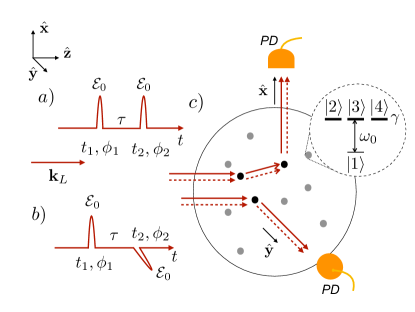
Figure 1: Setup for the observation of multiple quantum coherence (MQC) signals. Two phase-tagged (by phases $\phi_{1}$ and $\phi_{2}$), femtosecond, pump and probe laser pulses with variable time delay $\tau=t_{2}-t_{1}$ (also see fig. 2) propagate along the $z$ axis defined by the wave vector ${\mathbf{k}}_{\mathrm{L}}$. The pulses have (a) parallel linear polarizations along the $x$-axis; (b) orthogonal linear polarizations along the $x$- and $y$-axes, respectively. (c) Disordered sample of identical atomic scatterers with electronic dipole transition $J_{\mathrm{g}}=0\rightarrow J_{\rme}=1$ at frequency $\omega_{0}$, and spontaneous decay rate $\gamma$ of each excited state sublevel $|2\rangle$, $|3\rangle$, $|4\rangle$. Solid arrows represent incident and scattered field amplitudes, dashed ones the associated complex conjugates. Sequences of red arrows and black dots illustrate single and double scattering processes that contribute to the fluorescence signals collected by the photodetectors (PD) in the observation directions $\hat{\mathbf{y}}$ and $\hat{\mathbf{x}}$, respectively.

We consequently interpret MQC components distilled from the total fluorescence signal as arising from the multiple scattering of real photons between distant atoms.

Below, we recall the basics of the phase-modulated spectroscopy that was employed to measure MQC signals in dilute thermal gases [15, 18, 28]. Thereafter, we present our formalism and derive 1QC (single quantum coherence) and 2QC (double quantum coherence) spectra that are in excellent qualitative and reasonable quantitative agreement with experiment [18]. Ultimately, we establish the crucial role of radiative dipole-dipole interactions in the emergence of 2QC signals, which are impossible to observe for independent atoms – in agreement with [17], and we show that a system of two dipole interacting atoms is sufficient for modelling 1QC and 2QC signals – as a consequence of double scattering of real photons – in a dilute thermal gas. We especially highlight collective decay processes as an essential part of the dipolar interactions, without which qualitative agreement with the experiment cannot be achieved.

We now delve into a thorough presentation of the theory; the reader who is already familiar with the topic may take a shortcut to section 5, where we present our results.

2 Phase-modulated spectroscopy

In figure 1 we sketch the spectroscopy experiment used to extract the MQC signals. A thermal ensemble of alkali atoms is excited near-resonantly [15, 18] by two subsequent laser pulses injected at times $t_{1}$ and $t_{2}>t_{1}$, respectively [29]. The fluorescence subsequently emitted by the sample is collected by a photodetector in a direction orthogonal to the exciting field’s wave vector ${\bf k}_{\rm L}$. This excitation and detection procedure is repeated for $M_{\mathrm{cyc}}\gg 1$ cycles of duration $T_{\mathrm{cyc}}$, with the two pulses garnished with distinct phase tags $\phi_{1}$ and $\phi_{2}$, respectively, which are linearly ramped over subsequent cycles, with distinct rates $w_{1}\neq w_{2}$. These slowly evolving phase tags will turn out to be instrumental to distill the MQC signals from the total fluorescence. $T_{\mathrm{cyc}}$ is chosen to significantly exceed the atomic radiative lifetime of a few tens of nanoseconds [30], such that the atoms decay to the ground state [15, 18] within a single cycle, and each of the $M_{\mathrm{cyc}}$ cycles can be considered in isolation (see fig. 2).

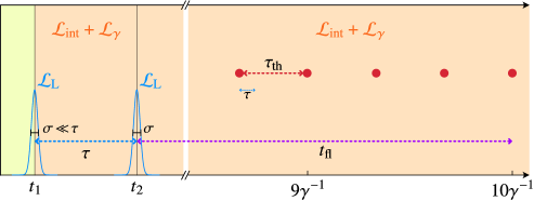
Figure 2: Schematic illustration of the different time scales and of the associated Liouvillians, for a single experimental cycle of duration $T_{\mathrm{cyc}}$. Two ultrashort Gaussian laser pulses with the same width $\sigma$ arrive at times $t_{1}$ and $t_{2}$, separated by a delay $\tau\gg\sigma$. After the second pulse, fluorescence is monitored during the interval $t_{\mathrm{fl}}\sim 10\gamma^{-1}\gg\tau$, until all atoms decay into the ground state. The fluorescence detection time $t_{\mathrm{fl}}$ is much longer than the thermal decoherence time $\tau_{\rm th}>\tau$, beyond which the atomic motion cannot be ignored. During the ultrashort laser-atom interaction, the dynamics of the atomic operators $Q(t)$ in (12) is governed by the Liouvillian $\mathscr{L}_{\mathrm{L}}$. Instead, $\mathscr{L}_{\mathrm{int}}$ and $\mathscr{L}_{\gamma}$ generate the dynamics during the intervals $\tau$ and $t_{\mathrm{fl}}$.

To resolve the details of the excitation scheme, we focus on the $m$th cycle ($0\leq m<M_{\mathrm{cyc}}$), which begins at $\tau_{m}=mT_{\mathrm{cyc}}$. For positive delays $t\in[0,T_{\mathrm{cyc}}]$ with respect to $\tau_{m}$, and in the frame co-rotating with the laser carrier frequency $\omega_{\mathrm{L}}$, the injected field has the time-dependent amplitude

$${\mathbf{E}}_{\mathrm{L}}(\mathbf{r},t)=\sum_{j=1}^{2}\bm{\varepsilon}_{\mathrm{L}}^{(j)}{\cal E}_{\mathrm{L}}(t-t_{j})\rme^{\rmi({\mathbf{k}}_{\mathrm{L}}\cdot\mathbf{r}+\omega_{\mathrm{L}}t_{j}+\phi_{j})}\,,$$ (1)

with the same Gaussian envelope ${\cal E}_{\mathrm{L}}(t^{\prime})={\cal E}_{0}\exp(-t^{\prime 2}/2\sigma^{2})$ of both incoming pulses, amplitude ${\cal E}_{0}$ and duration $\sigma$. Each phase tag $\phi_{j}=w_{j}(\tau_{m}+t)$ can be approximated by $\phi_{j}\approx w_{j}\tau_{m}$ for modulation frequencies $w_{j}\ll\omega_{L}$ [29] , and is imprinted on the respective pulse by transmission through an acousto-optical modulator oscillating at frequency $w_{j}$. Both pulses are collinear, with wave vector $\mathbf{k}_{\mathrm{L}}$, but may have different polarizations $\bm{\varepsilon}_{\mathrm{L}}^{(j)}$: in the following we consider the cases $\bm{\varepsilon}_{\mathrm{L}}^{(1)}=\bm{\varepsilon}_{\mathrm{L}}^{(2)}=\hat{\mathbf{x}}$, as well as $\bm{\varepsilon}_{\mathrm{L}}^{(1)}=\hat{\mathbf{x}}$ and $\bm{\varepsilon}_{\mathrm{L}}^{(2)}=\hat{\mathbf{y}}$. In a typical experiment, $\sigma\sim$50\text{\,}\mathrm{fs}$\ll\tau=t_{2}-t_{1}\sim$10\text{\,}\mathrm{ps}$\ll T_{\mathrm{cyc}}\sim$300\text{\,}\mathrm{\SIUnitSymbolMicro s}$$.

As a consequence of the phase tagging of the driving field, the transient fluorescence intensity $I_{\hat{\mathbf{k}}}(\tau,t_{\rm fl},\phi_{1},\phi_{2})$ in the direction $\hat{\mathbf{k}}\perp{\bf k}_{\rm L}$ exhibits a modulation – in its dependence on $\tau_{m}$ through $\phi_{1}$ and $\phi_{2}$ – at the frequency difference $w_{21}=w_{2}-w_{1}$, and at higher harmonics thereof, with the $\kappa$th harmonic identifying the $\kappa$th quantum coherence ($\kappa$QC) [15]. So does the time-integrated (over the $m\rm th$ cycle) fluorescence signal as collected in the far field over times $t_{2}+t_{\rm fl}$, with $0\leq t_{\rm fl}\leq T_{\mathrm{cyc}}-t_{2}\gg\gamma^{-1}$, $\gamma$ the natural line width of the atomic excited states, faithfully approximated by

$$\bar{I}_{\hat{\mathbf{k}}}(\tau,\phi_{1},\phi_{2})=\int_{0}^{\infty}\mathinner{\rmd t_{\rm fl}}I_{\hat{\mathbf{k}}}(\tau,t_{\rm fl},\phi_{1},\phi_{2})\,.$$ (2)

When incident on a photodetector, the integrated signal generates a photocurrent proportional to $\bar{I}_{\hat{\mathbf{k}}}(\tau,\phi_{1},\phi_{2})$, which (independently) depends on the pulse delay $\tau$, and – via the phase tags $\phi_{1},\phi_{2}$ (see above) – on the cycling time $\tau_{m}$. Frequency analysis of the photocurrent with respect to $\tau_{m}$, to distill the targeted order $\kappa$ of MQC, and with respect to $\tau$, to extract the $\kappa\rm QC$ signal strength at the characteristic frequency $\kappa\omega_{0}$ completes the experimental protocol, as elaborated in Sec. 4.4.5 below.

3 Theoretical model

3.1 Hamiltonian

Typical experiments to sense MQC signals are carried out at room temperatures with atomic clouds of low densities $\rho\sim${10}^{7}\text{\,}\mathrm{-}$${10}^{11}\text{\,}{\mathrm{cm}}^{-3}$$ [15, 18]. These are very dilute gases for which $\rho k_{0}^{-3}\ll 1$, with the atoms typically in the far-field of each other. Given that collisional broadening (see, e.g., [31]) in such ensembles is at least one order of magnitude narrower than the natural line width [28], we can neglect collisions between the atoms to a good approximation.

Our model considers $N$ identical, initially unexcited atoms at random positions $\mathbf{r}_{\alpha}(t)={\bf r}_{\alpha 0}+{\bf v}_{\alpha}t$, where ${\bf r}_{\alpha 0}$ and ${\bf v}_{\alpha}$ are, respectively, the initial coordinate and velocity of atom $\alpha=1,\ldots,N$. We assume a homogeneous and isotropic distribution of the initial coordinates ${\bf r}_{\alpha 0}$ (which implements the above far-field configuration), while the Cartesian components of the velocities ${\bf v}_{\alpha}$ can be drawn from the Maxwell-Boltzmann distribution corresponding to the temperature of the cloud. At typical room temperatures the atomic velocity is $\sim${10}^{2}\text{\,}\mathrm{m}\text{/}\mathrm{s}$$; hence, the atomic momentum is much larger (for ⁸⁷Rb atoms probed in [18], by about three orders of magnitude) than the photon momentum. Under this condition we can neglect the recoil effect and treat the atomic motion classically.

Then, the total Hamiltonian of the atomic ensemble interacting with an electromagnetic bath represented by an infinite set of quantized harmonic oscillators in their vacuum state, and with the classical, near-resonant pump and probe pulses (1) reads

$$H=H_{0}+H_{\mathrm{F}}+H_{\mathrm{AF}}+H_{\mathrm{AL}},$$ (3)

where

• $H_{0}=\sum_{\alpha=1}^{N}\hbar\omega_{0}{\bf D}_{\alpha}^{\dagger}\cdot{\bf D}_{\alpha}$ defines the free atoms’ Hamiltonian, with $\omega_{0}\approx\omega_{\mathrm{L}}$, and $\textbf{D}^{\dagger}_{\alpha}$ ($\textbf{D}_{\alpha}$) the atomic raising (lowering) operators incorporating arbitrary degeneracies of the ground and excited state sublevels.

• $H_{\mathrm{F}}=\sum_{{\bf k}s}\hbar\omega_{k}a^{\dagger}_{{\bf k}s}a_{{\bf k}s}$ describes the contribution from the quantized, free electromagnetic environment, with $a^{\dagger}_{{\bf k}s}$ ($a_{{\bf k}s}$) the creation (annihilation) operator of a photon with wave vector ${\bf k}$ and polarization $s$.

• $H_{\mathrm{AL}}$ and $H_{\mathrm{AF}}$ mediate the coupling between the atomic degrees of freedom and, respectively, the injected laser field and the quantized field. We employ the electric dipole approximation to write the Hamiltonians $H_{\mathrm{AL}}$ and $H_{\mathrm{AF}}$ as

  $$H_{\mathrm{AL}} = {-d}\sum_{\alpha=1}^{N}{\bf D}_{\alpha}^{\dagger}\cdot{\bf E}_{\mathrm{L}}({\bf r}_{\alpha}(t),t)\mathinner{\rme^{-\rmi\omega_{\mathrm{L}}t}}+{\rm h.c.},$$ (4)

  $$H_{\mathrm{AF}} = {-d}\sum_{\alpha=1}^{N}{\bf D}_{\alpha}^{\dagger}\cdot\Bigl{(}\mathbf{E}^{(+)}(\mathbf{r}_{\alpha}(t))+\mathbf{E}^{(-)}(\mathbf{r}_{\alpha}(t))\Bigr{)}+{\rm h.c.},$$ (5)

  where $d$ is the atomic dipole matrix element [31], which is assumed to be real, without loss of generality, ${\mathbf{E}}_{\mathrm{L}}(\mathbf{r}_{\alpha}(t),t)$ is given by (1) and ${\bf E}^{(+/-)}({\bf r}_{\alpha}(t))$ is the positive/negative-frequency part of the quantized field given by

  $${\bf E}^{(+)}({\bf r})=\rmi\sum_{{\bf k}s}\left(\frac{\hbar\omega_{k}}{2\epsilon_{0}V}\right)^{1/2}\bm{\varepsilon}_{{\bf k}s}a_{{\bf k}s}\rme^{\rmi{\bf k}\cdot{\bf r}},\qquad{\bf E}^{(-)}=\Bigl{(}{\bf E}^{(+)}\Bigr{)}^{\dagger},$$ (6)

  with $\epsilon_{0}$ the free space permittivity, $V$ the quantization volume, and $\bm{\varepsilon}_{{\bf k}s}$ the polarization vector. In Eq. (4) for $H_{\mathrm{AL}}$, we have additionally applied the rotating-wave (resonant) approximation, whereas counter-rotating terms must be kept in Eq. (5) for $H_{\mathrm{AF}}$ to obtain correct collective level shifts [32, 33, 34].

MQC signals were observed [18] in ⁸⁷Rb vapours, with the probed transitions endowed with fine and hyperfine structures, leading to rich multi-component features of the signals. We here ignore these features and specialize to atoms equipped with a $J_{\mathrm{g}}=0\rightarrow J_{\rme}=1$ transition, which involves a non-degenerate ground state and three sublevels in the excited state (see figure 1). While this simplifies our model with respect to the ⁸⁷Rb experiment [18], it still incorporates the experimentally important excited state degeneracy (a feature already employed earlier [24, 25, 26] to account for the relevant optical transition ${}^{1}S_{0}\rightarrow\,^{1}P_{1}$ in experiments on the coherent backscattering of light by cold strontium atoms [35]). A crucial consequence thereof is the presence of levels that are not driven by the polarized laser fields, but still can be populated by the dipole-dipole interaction. Such processes can be identified using different pump-probe polarizations and observation directions  [18]. Unlike previous treatments based on two-level atoms without any internal degeneracy [13, 16, 17, 36, 37, 38], our model is adequate to capture the consequences of this redistribution of energy between angular momentum states.

The atomic lowering operator associated with a $J_{\mathrm{g}}=0\rightarrow J_{\rme}=1$ transition is given by

$$\textbf{D}_{\alpha}=-\hat{\mathbf{e}}_{-1}\sigma_{12}^{\alpha}+\hat{\mathbf{e}}_{0}\sigma_{13}^{\alpha}-\hat{\mathbf{e}}_{+1}\sigma_{14}^{\alpha},$$ (7)

where $\sigma_{lk}^{\alpha}=|l\rangle_{\alpha}\langle k|_{\alpha}$, the excited state sublevels $|2\rangle$, $|3\rangle$, $|4\rangle$ (see figure 1) have magnetic quantum numbers $-1,0,+1$, and couple to field polarizations ${\hat{\mathbf{e}}_{-1}=(\hat{\mathbf{x}}-\rmi\hat{\mathbf{y}})/\sqrt{2}}$, ${\hat{\mathbf{e}}_{0}=\hat{\mathbf{z}}}$, and ${\hat{\mathbf{e}}_{+1}=-(\hat{\mathbf{x}}+\rmi\hat{\mathbf{y}})/\sqrt{2}}$, respectively.

Note that, in equation (3), we omit the kinetic energy of the atomic centre-of-mass motion, as well as atomic contact interaction terms [39], which must be taken into account in dense atomic systems, where $\rho k_{0}^{-3}\gtrsim 1$, but can be safely neglected in dilute ensembles [40].

3.2 Fluorescence intensity

The experimentally detected total signal is expressed through the quantum-mechanical expectation value of the intensity operator, averaged over atomic configurations,

$$I_{\hat{\mathbf{k}}}(t)=\Bigl{\langle}\bigl{\langle}\mathbf{E}^{(-)}_{\hat{\mathbf{k}}}(t)\cdot\mathbf{E}^{(+)}_{\hat{\mathbf{k}}}(t)\bigr{\rangle}\Bigr{\rangle}_{\mathrm{conf}}\,,$$ (8)

where $\langle\ldots\rangle=\mathop{\mathrm{Tr}}\{\ldots\varrho(0)\}$. The initial density operator $\varrho(0)$ of the atom-field system factorises into the ground state of the atoms and the vacuum state of the field. The positive frequency part ${\mathbf{E}}^{(+)}_{\hat{\mathbf{k}}}(t)$ of the operator for the electric far-field can be expressed through the atomic lowering operator of the source atoms  [41, 42],

$${\mathbf{E}}^{(+)}_{\hat{\mathbf{k}}}(t)=f\sum_{\alpha=1}^{N}\Bigl{\{}\textbf{D}_{\alpha}(t)-\hat{\mathbf{k}}\bigl{[}\hat{\mathbf{k}}\cdot\textbf{D}_{\alpha}(t)\bigr{]}\Bigr{\}}\rme^{-\rmi\textbf{k}\cdot\mathbf{r}_{\alpha}(t)}\,,$$ (9)

where $f=\omega_{0}^{2}d/(4\pi\epsilon_{0}c^{2}R_{d})$, $c$ is the speed of light, $R_{d}$ is the distance from the center of mass of the cloud to the detector, and ${\mathbf{k}}$ is the wave vector of the scattered light. In writing (9), we assumed that $R_{d}\gg r_{\alpha\beta}(t)=|\mathbf{r}_{\alpha}(t)-\mathbf{r}_{\beta}(t)|$ for any $\alpha$, $\beta$. Finally, $\langle\ldots\rangle_{\mathrm{conf}}$ stands for the configuration (or disorder) average. It results from the random initial positions of the atoms within the cloud, and from their thermal motion during the fluorescence detection time $t_{\rm fl}$. We will treat the thermal motion effectively, through configuration averaging which involves an integration over the length and direction of the vectors $\mathbf{r}_{\alpha\beta}$ connecting pairs of atoms (see section 4.4.4 for more details), with mean interatomic distance $\bar{r}$.

Plugging (9) into (8), with atomic levels from (7), and $\mathbf{k}=k\hat{\mathbf{x}}$, we obtain

$$I_{\hat{\mathbf{x}}}=\biggl{\langle}f^{2}\sum_{\mathchoice{{}\hbox to0.0pt{\hss$\displaystyle{\alpha,\beta=1}$\hss}}{{}\hbox to0.0pt{\hss$\textstyle{\alpha,\beta=1}$\hss}}{{}\hbox to0.0pt{\hss$\scriptstyle{\alpha,\beta=1}$\hss}}{{}\hbox to0.0pt{\hss$\scriptscriptstyle{\alpha,\beta=1}$\hss}}}^{N}\rme^{\rmi k\hat{\mathbf{x}}\cdot\mathbf{r}_{\alpha\beta}}\Bigl{(}\langle\sigma_{z1}^{\alpha}\sigma_{1z}^{\beta}\rangle+\langle\sigma_{y1}^{\alpha}\sigma_{1y}^{\beta}\rangle\Bigr{)}\biggr{\rangle}_{\mathrm{conf}}$$ (10)

and $I_{\hat{\mathbf{y}}}$ follows upon replacing $\hat{\mathbf{x}}\rightarrow\hat{\mathbf{y}}$, $y\rightarrow x$ in (10). Note that, in the above equation, we dropped the time argument and introduced a new (degenerate) atomic excited manifold basis,

$$|x\rangle=(|4\rangle-|2\rangle)/\sqrt{2},\quad|y\rangle=(|4\rangle+|2\rangle)/(\sqrt{2}\rmi),\quad|z\rangle=|3\rangle.$$ (11)

3.3 Master equation

Evaluation of the fluorescence intensity (10) includes certain time-dependent atomic dipole correlators like $\langle\sigma_{z1}^{\alpha}\sigma_{1z}^{\beta}\rangle$. For immobile atoms it is technically involved, though fundamentally straightforward, to derive a Lehmberg-type master equation for an arbitrary atomic operator [43] (or, equivalently, for the atomic density operator [41]) under the standard Born and Markov approximations [23]. Such a master equation contains a Liouvillian describing the dipole-dipole coupling, which is a function of the distance $r_{\alpha\beta}$ between the interacting particles. In a thermal ensemble, the interatomic distance is time-dependent, such that employing the standard approximations in this regime requires justification. As it turns out, the Born and Markov approximations may also prevail for moving atoms—provided that the Doppler shift $k_{0}v_{\alpha}$ ($v_{\alpha}=|{\bf v}_{\alpha}|$ and $k_{0}=\omega_{0}/c$) amounts to a negligibly small phase shift $k_{0}v_{\alpha}r_{\alpha\beta}(t)/c\ll 1$ during the propagation time $r_{\alpha\beta}(t)/c$ of the interaction between the atoms [34]. In other words, the atoms can be considered “frozen” on the time scale $r_{\alpha\beta}(t)/c$. This condition is well satisfied, for example, for $r_{\alpha\beta}(t)=\bar{r}\sim$10\text{\,}\mathrm{\SIUnitSymbolMicro m}$$ and a Doppler shift $k_{0}v_{\alpha}\sim$600\text{\,}\mathrm{MHz}$$, since $k_{0}v_{\alpha}r_{\alpha\beta}(t)/c\sim 2\times 10^{-5}$. We therefore obtain the same form of the dipole-dipole interaction as for fixed atoms, where $r_{\alpha\beta}$ is substituted by $r_{\alpha\beta}(t)$ [34].

Thus, an arbitrary time-dependent atomic dipole correlator can be obtained from the quantum master equation [42, 43] (written in the interaction picture with respect to the free-atom Hamiltonian $H_{0}$):

$$\dot{Q}=(\mathscr{L}_{\mathrm{L}}+\mathscr{L}_{\gamma}+\mathscr{L}_{\mathrm{int}})Q,$$ (12)

where $Q$ is an arbitrary atomic operator (on the space of $N$ atoms) averaged over the free field subsystem, $\mathscr{L}_{\mathrm{L}}=\sum_{\alpha=1}^{N}\mathscr{L}_{\mathrm{L}}^{\alpha}$, with $\mathscr{L}_{\mathrm{L}}^{\alpha}$ the laser-atom interaction Liouvillian; $\mathscr{L}_{\gamma}=\sum_{\alpha=1}^{N}\mathscr{L}_{\gamma}^{\alpha}$, with $\mathscr{L}_{\gamma}^{\alpha}$ the Lindblad superoperator describing the atomic relaxation due to the electromagnetic bath; and $\mathscr{L}_{\mathrm{int}}=\sum_{\alpha\neq\beta=1}^{N}\mathscr{L}_{\alpha\beta}$, with $\mathscr{L}_{\alpha\beta}$ the Liouvillian describing the dipole-dipole interactions mediated by the (common) electromagnetic bath. The Liouvillians read [24, 25, 33, 42]

$$\mathscr{L}_{\mathrm{L}}^{\alpha}Q = -\frac{\rmi d}{\hbar}\bigl{[}{\mathbf{D}}_{\alpha}^{\dagger}\cdot{\mathbf{E}}_{\mathrm{L}}(\mathbf{r}_{\alpha 0},t)\rme^{-\rmi\delta_{\alpha}t}+{\mathbf{D}}_{\alpha}\cdot{\mathbf{E}}^{*}_{\mathrm{L}}(\mathbf{r}_{\alpha 0},t)\rme^{\rmi\delta_{\alpha}t},Q\bigr{]},$$ (13)

$$\mathscr{L}_{\gamma}^{\alpha}Q = \frac{\gamma}{2}\Bigl{(}\textbf{D}^{\dagger}_{\alpha}\cdot\bigl{[}Q,\textbf{D}_{\alpha}\bigr{]}+\bigl{[}\textbf{D}^{\dagger}_{\alpha},Q\bigr{]}\cdot\textbf{D}_{\alpha}\Bigr{)},$$ (14)

with

$$\delta_{\alpha}=\omega_{\mathrm{L}}-\omega_{0}-\mathbf{k}_{\mathrm{L}}\cdot\mathbf{v}_{\alpha}$$ (15)

the laser-atom detuning incorporating the Doppler shift of the atomic transition frequency, $\gamma$ the spontaneous decay rate (identical for all excited state levels), and

$$\mathscr{L}_{\alpha\beta}Q=\textbf{D}^{\dagger}_{\alpha}\!\cdot\!\overset{\text{\tiny$\bm{\leftrightarrow}$}}{\mathbf{T}}(k_{0}r_{\alpha\beta}(t),\hat{\mathbf{n}})\!\cdot\!\bigl{[}Q,\textbf{D}_{\beta}\bigr{]}+\bigl{[}\textbf{D}^{\dagger}_{\beta},Q\bigr{]}\!\cdot\!\overset{\text{\tiny$\bm{\leftrightarrow}$}}{\mathbf{T}}{}^{*}(k_{0}r_{\alpha\beta}(t),\hat{\mathbf{n}})\!\cdot\!\textbf{D}_{\alpha}\,,$$ (16)

with the dipole-dipole interaction tensor $\overset{\text{\tiny$\bm{\leftrightarrow}$}}{\mathbf{T}}(k_{0}r_{\alpha\beta}(t),\hat{\mathbf{n}})$ which, with $\hat{\mathbf{n}}=\mathbf{r}_{\alpha\beta}/r_{\alpha\beta}=(\sin\theta\cos\phi,\sin\theta\sin\phi,\cos\theta)$ and $\xi(t)=k_{0}r_{\alpha\beta}(t)$, reads

$$\overset{\text{\tiny$\bm{\leftrightarrow}$}}{\mathbf{T}}(\xi(t),\hat{\mathbf{n}})=\frac{3\gamma}{4}\rme^{-\rmi\xi(t)}\left[\frac{\rmi}{\xi(t)}\Bigl{(}\mathbbm{1}-\hat{\mathbf{n}}\hat{\mathbf{n}}\Bigr{)}+\left(\frac{1}{\xi(t)^{2}}-\frac{\rmi}{\xi(t)^{3}}\right)\Bigl{(}\mathbbm{1}-3\hat{\mathbf{n}}\hat{\mathbf{n}}\Bigr{)}\right].$$ (17)

In this equation, $\mathbbm{1}$ is a $3\times 3$ unit matrix and $\hat{\mathbf{n}}\hat{\mathbf{n}}$ is a $3\times 3$ dyadic. Since we assume linear polarization of the incoming laser pulses, it is most convenient to express the matrix elements of $\overset{\text{\tiny$\bm{\leftrightarrow}$}}{\mathbf{T}}(\xi(t),\hat{\mathbf{n}})$ in the Cartesian basis, $\overset{\text{\tiny$\bm{\leftrightarrow}$}}{\mathbf{T}}_{kl}=\hat{\mathbf{e}}_{k}\cdot\overset{\text{\tiny$\bm{\leftrightarrow}$}}{\mathbf{T}}\cdot\hat{\mathbf{e}}_{l}$, $k,l\in\{x,y,z\}$.

3.4 Near- versus far-field form of the dipole-dipole interaction

Note that the near-field term in equation (17), scaling as $\xi^{-3}$ (we drop for brevity the time argument), is the $\xi\ll 1$ asymptote of the dipole-dipole coupling tensor (17) [43], and is associated with the electrostatic interaction. It is this form of the interaction that was employed in all previous theoretical treatments dealing with MQC signals in dilute atomic gases [13, 17, 36, 37, 38], where atomic angular momentum was also ignored.

To identify the associated form of dipolar interactions, we consider a simple two-level atomic structure rather than our $J_{\mathrm{g}}=0\rightarrow J_{\rme}=1$ transition, i.e. we keep only level $|3\rangle$ in the excited state manifold. The tensor (17) then reduces to its matrix element $\overset{\text{\tiny$\bm{\leftrightarrow}$}}{\mathbf{T}}_{zz}$ corresponding to the magnetic number zero, which, in the near-field limit $\propto\xi^{-3}$, reads

$$\overset{\text{\tiny$\bm{\leftrightarrow}$}}{\mathbf{T}}_{zz}=-\frac{3\gamma\rmi}{4}\frac{1-3\cos^{2}\theta}{\xi^{3}}.$$ (18)

Recalling the definition $\gamma=4\omega_{0}^{3}d^{2}/(4\pi\epsilon_{0}3\hbar c^{2})$ [31], and introducing the dipole moment operators $\mathbf{d}(\sigma_{13}+\sigma_{31})$ of the two-level systems, with $\mathbf{d}=d\hat{\mathbf{e}}_{z}$, equations (12), (16) and (18) lead to the following Heisenberg equation of motion for two atoms $\alpha$ and $\beta$:

$$\dot{Q}=\frac{\rmi}{\hbar}\Biggl{[}\underbrace{\frac{1}{4\pi\epsilon_{0}}\frac{{\mathbf{d}}^{2}-3({\mathbf{d}}\cdot{\hat{\mathbf{n}}})^{2}}{r_{\alpha\beta}^{3}}}_{V_{\text{d-d}}}\sigma_{31}^{\alpha}\sigma_{13}^{\beta},Q\Biggr{]},$$ (19)

where we have identified the electrostatic dipole-dipole interaction $V_{\text{d-d}}$. We can see from equation (19) that the interatomic potential $V_{\text{d-d}}$ generates purely Hamiltonian dynamics, which does not affect the ground and doubly excited states $|1\rangle_{\alpha}|1\rangle_{\beta}$ and $|3\rangle_{\alpha}|3\rangle_{\beta}$, respectively, of the uncoupled system. It does, however, shift both uncoupled single-excitation eigenstates $|3\rangle_{\alpha}|1\rangle_{\beta}$ and $|1\rangle_{\alpha}|3\rangle_{\beta}$. In quantum electrodynamics, these shifts are interpreted as originating from the exchange of virtual photons [39].

In contrast to the electrostatic part (19) of the interaction, its radiative part accounts for the exchange of real, or transverse, photons [39], and generates both, collective shifts and collective decay of the atomic excited states, associated, respectively, with the tensors $\overset{\text{\tiny$\bm{\leftrightarrow}$}}{\mathbf{\Omega}}(\xi,\hat{\mathbf{n}})=\mathop{\mathrm{Im}}\overset{\text{\tiny$\bm{\leftrightarrow}$}}{\mathbf{T}}(\xi,\hat{\mathbf{n}})$ and $\overset{\text{\tiny$\bm{\leftrightarrow}$}}{\mathbf{\Gamma}}(\xi,\hat{\mathbf{n}})=\mathop{\mathrm{Re}}\overset{\text{\tiny$\bm{\leftrightarrow}$}}{\mathbf{T}}(\xi,\hat{\mathbf{n}})$. While $\overset{\text{\tiny$\bm{\leftrightarrow}$}}{\mathbf{\Gamma}}(\xi,\hat{\mathbf{n}})=0$ in the near-field limit (19), we here are dealing with dilute gases characterized by interatomic distances that are much larger than the optical wavelength. Consequently, in the far-field limit $\xi\gg 1$, the tensor $\overset{\text{\tiny$\bm{\leftrightarrow}$}}{\mathbf{T}}$ retains its real and imaginary parts, scaling as $\xi^{-1}$, by equation (17). In that limit, $\overset{\text{\tiny$\bm{\leftrightarrow}$}}{\mathbf{T}}(\xi,\hat{\mathbf{n}})\approx(3\gamma/4)g(\xi)[\mathbbm{1}-\hat{\mathbf{n}}\hat{\mathbf{n}}]$, with coupling parameter $g(\xi)=\rmi\rme^{-\rmi\xi}/\xi$, $|g(\xi)|\ll 1$, and decay rates and level shifts can be deduced from

$$\overset{\text{\tiny$\bm{\leftrightarrow}$}}{\mathbf{\Gamma}}(\xi,\hat{\mathbf{n}})=\frac{3\gamma}{4}\frac{\sin\xi}{\xi}(\mathbbm{1}-\hat{\mathbf{n}}\hat{\mathbf{n}}),\qquad\overset{\text{\tiny$\bm{\leftrightarrow}$}}{\mathbf{\Omega}}(\xi,\hat{\mathbf{n}})=\frac{3\gamma}{4}\frac{\cos\xi}{\xi}(\mathbbm{1}-\hat{\mathbf{n}}\hat{\mathbf{n}}),$$ (20)

which are both oscillating functions of $\xi$, with identical amplitude. This means that both terms contribute equally to the dynamics and, hence, the non-Hermititian dissipative terms generated by $\overset{\text{\tiny$\bm{\leftrightarrow}$}}{\mathbf{\Gamma}}(\xi,\hat{\mathbf{n}})$ cannot be neglected.

With the definition (20) of $\overset{\text{\tiny$\bm{\leftrightarrow}$}}{\mathbf{\Gamma}}$ and $\overset{\text{\tiny$\bm{\leftrightarrow}$}}{\mathbf{\Omega}}$, the interaction Liouvillian from (16) can be decomposed as ${\cal L}_{\alpha\beta}={\cal L}^{(1)}_{\alpha\beta}+{\cal L}^{(2)}_{\alpha\beta}$, with

$${\cal L}^{(1)}_{\alpha\beta}Q = -\rmi\textbf{D}^{\dagger}_{\alpha}\!\cdot\!(\overset{\text{\tiny$\bm{\leftrightarrow}$}}{\mathbf{\Omega}}-\rmi\overset{\text{\tiny$\bm{\leftrightarrow}$}}{\mathbf{\Gamma}})\!\cdot\!\textbf{D}_{\beta}Q+\rmi Q\textbf{D}^{\dagger}_{\alpha}\!\cdot\!(\overset{\text{\tiny$\bm{\leftrightarrow}$}}{\mathbf{\Omega}}+\rmi\overset{\text{\tiny$\bm{\leftrightarrow}$}}{\mathbf{\Gamma}})\!\cdot\!\textbf{D}_{\beta},$$ (21)

$${\cal L}^{(2)}_{\alpha\beta}Q = 2\textbf{D}^{\dagger}_{\alpha}\!\cdot\!\overset{\text{\tiny$\bm{\leftrightarrow}$}}{\mathbf{\Gamma}}\!\cdot\!Q\textbf{D}_{\beta}.$$ (22)

This distinction between contributions to ${\cal L}_{\alpha\beta}$ will be essential for our interpretation of MQC spectra in section 5 below. Let us therefore describe their action on specific operators $Q$ in detail:

• The operator part $(\textbf{D}^{\dagger}_{\alpha})_{r}(\textbf{D}_{\beta})_{j}=\sigma^{\alpha}_{r1}\sigma^{\beta}_{1j}$, ($r,j\in\{x,y,z\}$) of the Liouvillian ${\cal L}^{(1)}_{\alpha\beta}$ (see (21)) transfers one excitation from atom $\beta$ to atom $\alpha$. When $(\textbf{D}^{\dagger}_{\alpha})_{r}(\textbf{D}_{\beta})_{j}$ acts on the projector $Q=\sigma^{\alpha}_{11}\sigma^{\beta}_{ff}$ from the left (where ($f\in\{x,y,z\}$), it transforms the latter into the operator $Q^{\prime}=\delta_{jf}\sigma^{\alpha}_{r1}\sigma^{\beta}_{1f}$ of electronic coherences of both atoms. This transformation amounts to the dynamical equation $\dot{Q}=\sum_{rj}(-\rmi\overset{\text{\tiny$\bm{\leftrightarrow}$}}{\mathbf{\Omega}}_{rj}-\overset{\text{\tiny$\bm{\leftrightarrow}$}}{\mathbf{\Gamma}}_{rj})Q^{\prime}$, which couples the exited state populations to the electronic coherences. The action of $\sigma^{\alpha}_{r1}\sigma^{\beta}_{1j}$ from the right can be described analogously.

• Since the raising and lowering operators of different atoms in ${\cal L}^{(2)}_{\alpha\beta}$ (see (22)) act from the left and right side on an atomic operator, this Liouvillian performs the transformation to a two-atom subspace with an extra excitation. As a result, an operator $Q^{\prime}=\sigma^{\alpha}_{1j}\sigma^{\beta}_{r1}$ describing electronic coherences of both atoms is transformed into that of Zeeman coherences and excited state populations, $(\textbf{D}^{\dagger}_{\alpha})_{f}Q^{\prime}(\textbf{D}_{\beta})_{l}=\sigma^{\alpha}_{fj}\sigma^{\beta}_{rl}=Q^{\prime\prime}$ ($f,j,r,l\in\{x,y,z\}$). We can write this as a dynamical equation, $\dot{Q^{\prime}}=2\sum_{fl}\overset{\text{\tiny$\bm{\leftrightarrow}$}}{\mathbf{\Gamma}}_{fl}Q^{\prime\prime}$, stating that Zeeman coherences and excited state populations of two atoms (embodied in $Q^{\prime\prime}$) are transformed to their electronic coherences (embodied in $Q^{\prime}$) via a collective decay process.

4 Analytical solution of the master equation

4.1 Separation of time scales

Our approach to solve (12), with ingredients (13)-(17), analytically is based on the observation that the atomic dynamics during each experimental cycle (see figure 2) is characterized by four different time scales (recall section 2). The first, ultrashort time scale is set by the laser pulse length $\sigma\sim$50\text{\,}\mathrm{fs}$$ (which enters through (1)). The interpulse delay $\tau\sim$10\text{\,}\mathrm{p}\mathrm{s}$$, which parametrizes (2), determines the second, short time scale. After the second pulse, atomic fluorescence is collected until the end of the cycle, at time $T_{\mathrm{cyc}}$ (entering (2), via $\phi_{1}$ and $\phi_{2}$, through $\tau_{m}$), until all atoms relax into their ground states by emission of a photon. This stage of the fluorescence detection establishes the third time scale, which typically lasts for about four orders of magnitude longer than the short time scale—for several microseconds. Finally, within the long time scale, the typical thermal coherence time $\tau_{\mathrm{th}}$ [44] of the order of $10\text{\,}\mathrm{ns}$ defines the fourth time scale, which demarcates the regime of the atomic dynamics beyond which the Doppler effect is not negligible.

Such separation of time scales motivates a simplified version of (12), which decomposes into terms relevant at distinct time scales. We thus completely ignore the incoherent dynamics generated by $\mathscr{L}_{\gamma}$ and $\mathscr{L}_{\text{int}}$ during that ultrashort time scale, while, on longer time scales, we solve (12) including all terms from (13) and (16) except for the Liouvillians $\mathscr{L}_{\mathrm{L}}$ which generate the dynamics induced by the (on these long time scales) “kick”-like laser-atom interaction. The thus defined propagation over ultrashort and longer time scales is then interchanged twice, to cover a single experimental cycle of duration $T_{\mathrm{cyc}}$. This approach resembles a stroboscopic description of the dynamics familiar, e.g., from stroboscopic maps [45] or also from micromaser theory [46].

Furthermore, we need to blend in the atoms’ thermal motion, which can be safely neglected on the ultrashort and short time scales. The atomic configuration set by $\mathbf{r}_{\alpha 0}$ is therefore considered frozen on these time scales. On the long time scale, however, atomic motion does affect the dipole-dipole coupling $\mathscr{L}_{\rm int}$ via the then time-dependent interatomic vectors ${\mathbf{r}_{\alpha\beta}(t)=\mathbf{r}_{\alpha 0}-\mathbf{r}_{\beta 0}+(\mathbf{v}_{\alpha}-\mathbf{v}_{\beta})t}$. This leads to rapidly oscillating,  $r_{\alpha\beta}(t)$-dependent phase factors in certain terms of our solutions of (12), which average out for many repetitions of experimental cycles of duration $T_{\mathrm{cyc}}$, each of them being much longer than the thermal coherence time $\tau_{\mathrm{th}}$. Therefore, we effectively account for the thermal atomic motion by averaging over the atomic configurations. As a result, atomic dipole correlators in (10) with position-dependent phases vanish, regardless of the observation direction. In contrast, so-called incoherent terms [25], which do not exhibit such phases and correspond to  $\alpha=\beta$ in equation (10), prevail. We note that, although this reduces the observable to a sum of single-atom correlators, these are obtained from the solution of the master equation (12) for $N$ dipole-dipole interacting atoms. Therefore, through these interactions, the fluorescence intensity (10) still depends on the surrounding atoms. An analogous reasoning applies for the position-dependent phases in the coupling (17) and in the pulses’ envelope (see equation (1)), as will be detailed in section 4.4.3.

4.2 Dynamics of independent atoms: Single-atom case

In the following, we present our derivation of $I_{\hat{\mathbf{k}}}(t)$ from (8). For noninteracting atoms (that is, $\mathscr{L}_{\rm int}=0$), it suffices to find a solution of a single-atom equation, as we show in this subsection. The dynamical behaviour of $N$ atoms is then given by the tensor product of evolution laws for individual atoms, as we discuss in 4.3.

By equation (12), an arbitrary single-atom operator $Q_{\alpha}$ obeys the equation of motion

$$\dot{Q}_{\alpha}(t)=\left(\mathscr{L}_{\mathrm{L}}^{\alpha}(t)+\mathscr{L}_{\gamma}^{\alpha}\right)Q_{\alpha}(t),$$ (23)

where the Liouvillians on the right hand side of (23) are given by (13), (14).

4.2.1 Ultrashort time scale — atom-laser interaction.

As argued in section 4.1, during the ultrashort intervals of non-vanishing laser intensity around the pulses’ arrival times $t_{j}$, dissipation processes generated by $\mathscr{L}_{\gamma}^{\alpha}$ are insignificant. Hence, we need to solve the following equation of motion generated by the Liouvillian $\mathscr{L}_{\mathrm{L}}^{\alpha}$:

$$\dot{Q}_{\alpha}(t)=\mathscr{L}_{\mathrm{L}}^{\alpha}(t)Q_{\alpha}(t)=-\frac{\rmi}{2}\Omega_{\mathrm{L}}(t)[{\cal M}_{j}(t),Q_{\alpha}(t)],$$ (24)

where $\Omega_{\mathrm{L}}(t)=2d{\cal E}_{\mathrm{L}}(t-t_{j})/\hbar$ is the time-dependent (real-valued) Rabi frequency, and

$${\cal M}_{j}(t)=S^{\dagger}\rme^{\rmi\chi_{j}-\rmi\delta_{\alpha}t}+S\rme^{-\rmi\chi_{j}+\rmi\delta_{\alpha}t}\,.$$ (25)

This is a generalized atomic dipole operator (whose index $\alpha$ we drop for simplicity), with $S^{\dagger}={\bf D}^{\dagger}_{\alpha}\cdot\bm{\varepsilon}_{\mathrm{L}}$, $S={\bf D}_{\alpha}\cdot\bm{\varepsilon}_{\mathrm{L}}^{*}$ atomic raising and lowering operators, according to (7), and the time-independent phase

$$\chi_{j}={\bf k}_{\mathrm{L}}\cdot{\bf r}_{\alpha 0}+\omega_{\mathrm{L}}t_{j}+w_{j}\tau_{m}\,,$$ (26)

which includes the phase tag $w_{j}\tau_{m}$ proper, as well as the phases imprinted by the carrier frequency according to (1). The laser-atom detuning $\delta_{\alpha}$ is given by equation (15).

Since the interaction with the Gaussian laser pulses occurs instantaneously in comparison to all other time scales (see section 4.1 and fig. 2), these can be modelled by delta pulses carrying the same energy $E_{\rm pulse}$. Such pulses are characterised solely by their area

$$\vartheta=\int_{-\infty}^{\infty}\mathinner{\rmd t^{\prime}}\Omega_{\mathrm{L}}(t^{\prime}),$$ (27)

which can be found using the relation (see, for instance, [47]) between the energy and the intensity of a pulse,

$$E_{\rm pulse}=2\epsilon_{0}cw_{0}{\cal E}^{2}_{0}\int_{-\infty}^{\infty}\mathinner{\rmd t^{\prime}}\rme^{-(t^{\prime}/\sigma)^{2}}=2\epsilon_{0}cw_{0}{\cal E}_{0}^{2}\sigma\sqrt{\pi}\,,$$ (28)

with $w_{0}$ the laser beam’s cross-section. Solving (28) for the field amplitude ${\cal E}_{0}$, we obtain $\vartheta=2d(\sigma c\mu_{0}E_{\rm pulse}\sqrt{\pi}/w_{0})^{1/2}/\hbar$, with  $\mu_{0}$ the free space permeability.

Furthermore, under the delta pulse approximation, equation (24) is simplified by replacing $\Omega_{\mathrm{L}}(t)$ by a properly weighted Dirac delta-function, and using the well-known formula (see, e.g. [48]) $f(t)\delta(t-t_{j})=f(t_{j})\delta(t-t_{j})$. As a result, we can replace ${\cal M}_{j}(t)\rightarrow{\cal M}_{j}(t_{j})\equiv{\cal M}_{j}$, with

$${\cal M}_{j}=S^{\dagger}\rme^{\rmi\varphi_{j}}+S\rme^{-\rmi\varphi_{j}},$$ (29)

where

$$\varphi_{j}={\bf k}_{\mathrm{L}}\cdot{\bf r}_{\alpha 0}+\omega_{0}t_{j}+w_{j}\tau_{m}+\Delta_{\alpha}t_{j},$$ (30)

and $\Delta_{\alpha}={\bf k}_{\mathrm{L}}\cdot{\bf v}_{\alpha}$ is the Doppler shift of atom $\alpha$. Now, the action of a delta kick at time $t_{j}$ on an atom can be expressed through a unitary superoperator $R^{\alpha}_{j}$ as

$$Q_{\alpha}(t^{+}_{j})=R^{\alpha}_{j}Q_{\alpha}(t_{j}^{-})=\mathinner{\rme^{-\rmi\vartheta{\cal M}_{j}/2}}Q_{\alpha}(t_{j}^{-})\mathinner{\rme^{\rmi\vartheta{\cal M}_{j}/2}},$$ (31)

where $Q_{\alpha}(t_{j}^{-})$ ($Q_{\alpha}(t_{j}^{+})$) is the single-atom operator before (after) the kick.

We can deduce the transformation performed by $R^{\alpha}_{j}$ in an algebraic form. To that end, we notice that the operators $S^{\dagger}$ and $S$ on the right hand side of equation (25) are generalizations of the Pauli pseudo-spin operators $\sigma_{+}$ and $\sigma_{-}$ to the case of degenerate excited state sublevels. Therefore, the algebraic properties of $S^{\dagger}$, $S$ are similar to those of $\sigma_{+}$, $\sigma_{-}$. To illustrate this by an example, let us consider laser polarizations $\bm{\varepsilon}_{\mathrm{L}}=\hat{\mathbf{x}}$ and $\bm{\varepsilon}_{\mathrm{L}}=\hat{\mathbf{y}}$, for which the operator $S$ reads, respectively (see also (11)),

$$\hat{\mathbf{x}}:S=\frac{\sigma_{14}-\sigma_{12}}{\sqrt{2}},\quad\hat{\mathbf{y}}:S=\rmi\frac{\sigma_{14}+\sigma_{12}}{\sqrt{2}},$$ (32)

and the corresponding raising operators follow by Hermitian conjugation of (32). Using equations (25) and (32), we obtain

$${\cal M}_{j}^{2}=S^{\dagger}S+SS^{\dagger},$$ (33)

which is a projector onto the subspace of the laser-driven levels $|1\rangle$, $|2\rangle$, and $|4\rangle$. This implies

$${\cal M}_{j}^{2k+1}={\cal M}_{j},\quad{\cal M}_{j}^{2k+2}={\cal M}_{j}^{2},\quad k=0,1,2,\ldots,$$ (34)

and, hence,

$$\exp\Bigl{(}\pm\,\rmi\,\frac{\vartheta}{2}{\cal M}_{j}\Bigr{)}=\left(\mathbbm{1}-{\cal M}_{j}^{2}\right)+{\cal M}_{j}^{2}\cos\frac{\vartheta}{2}\pm\rmi{\cal M}_{j}\sin\frac{\vartheta}{2}.$$ (35)

The last two terms of the obtained result are formally equivalent to the known operator identity for two-level systems (see, e.g. [49]), and describe an azimuthal rotation on the Bloch sphere by an angle $\vartheta$. In addition, the (trivial) evolution of laser-undriven levels (in the basis (11), and for $\bm{\varepsilon}_{\mathrm{L}}=\hat{\mathbf{x}}$ ($\bm{\varepsilon}_{\mathrm{L}}=\hat{\mathbf{y}}$), these are the levels $|y\rangle$ and $|z\rangle$ ($|x\rangle$ and $|z\rangle$)) is included in (35) via the projector $\mathbbm{1}-{\cal M}_{j}^{2}$. With the aid of equations (35) and (25), we obtain [50] the following expansion for the superoperator $R_{j}^{\alpha}$ from (31):

$$R^{\alpha}_{j}=\sum_{p=-2}^{2}\rme^{\rmi p\varphi_{j}}R_{j}^{[p]},$$ (36)

with superoperators $R_{j}^{[p]}$ independent of $\varphi_{j}$, and defined by their action on a single-atom operator $Q_{\alpha}$:

$$\mathinner{R_{j}^{[0]}}Q_{\alpha} = \mathinner{\Pi_{\vartheta}}Q_{\alpha}\mathinner{\Pi_{\vartheta}}+\mathinner{S^{\dagger}_{\vartheta}}Q_{\alpha}\mathinner{S_{\vartheta}}+\mathinner{S_{\vartheta}}Q_{\alpha}\mathinner{S^{\dagger}_{\vartheta}},$$

$$\mathinner{R_{j}^{[+1]}}Q_{\alpha} = \rmi\left(\mathinner{\Pi_{\vartheta}}Q_{\alpha}\mathinner{S^{\dagger}_{\vartheta}}-\mathinner{S^{\dagger}_{\vartheta}}Q_{\alpha}\mathinner{\Pi_{\vartheta}}\right),$$

$$\mathinner{R_{j}^{[-1]}}Q_{\alpha} = \rmi\left(\mathinner{\Pi_{\vartheta}}Q_{\alpha}\mathinner{S_{\vartheta}}-\mathinner{S_{\vartheta}}Q_{\alpha}\mathinner{\Pi_{\vartheta}}\right),$$ (37)

$$\mathinner{R_{j}^{[+2]}}Q_{\alpha} = \mathinner{S^{\dagger}_{\vartheta}}Q_{\alpha}\mathinner{S^{\dagger}_{\vartheta}},$$

$$\mathinner{R_{j}^{[-2]}}Q_{\alpha} = \mathinner{S_{\vartheta}}Q_{\alpha}\mathinner{S_{\vartheta}},$$

where

$$\mathinner{\Pi_{\vartheta}}=\left(\mathbbm{1}-{\cal M}_{j}^{2}\right)+{\cal M}_{j}^{2}\cos\frac{\vartheta}{2},\qquad\mathinner{S_{\vartheta}}=S\sin\frac{\vartheta}{2}.$$ (38)

Equations (36) and  (4.2.1) are crucial for the subsequent analysis of MQC signals in section 4.4.5, since they depend on the modulated phase $\varphi_{j}$ given by (30). We note that the simple structure of the expansion (36) is a direct consequence of the RWA  [51] applied in the atom-laser Hamiltonian $H_{\mathrm{AL}}$ as given in (4).

While the decomposition (36) is general, in our scenario the atoms are initially unexcited. In this case, the atomic density operator after the first laser pulse does not feature factors $\rme^{\pm 2\rmi\varphi_{1}}$, which is important for the disorder average and signal demodulation (see section 4.4.4 and section 4.4.5). For the $\hat{\bf x}$-polarized pump pulse, using (11), (32), (36) and  (4.2.1), we deduce

$$R_{1,\hat{\bf x}}^{\alpha}|1\rangle\!\langle 1|=\left(\cos\frac{\vartheta}{2}|1\rangle-\rmi\rme^{\rmi\varphi_{1}}\sin\frac{\vartheta}{2}|x\rangle\right)\left(\cos\frac{\vartheta}{2}\langle 1|+\rmi\rme^{-\rmi\varphi_{1}}\sin\frac{\vartheta}{2}\langle x|\right),$$ (39)

where we additionally introduced the index $\hat{\bf x}$, to make the polarisation explicit, and $|x\rangle=S^{\dagger}|1\rangle$. The single-atom density operator after the pump pulse thus exhibits electronic coherences, modulated as $\rme^{\pm\rmi\varphi_{1}}$, and populations of the ground and excited state sublevels dependent on the pulse area.

In section 4.4.3 below, by combining delta-pulse excitations with the subsequent time evolution due to $\mathscr{L}_{\gamma}+\mathscr{L}_{\mathrm{int}}$, we obtain an analytical formula for the two-atom state after the second pulse. In fact, for typical interpulse delays $\tau\sim$10\text{\,}\mathrm{ps}$$, the dynamics generated by the Liouvillians $\mathscr{L}_{\gamma}$ and $\mathscr{L}_{\mathrm{int}}$ can be neglected to a good approximation. With this in mind, we can derive explicit expressions for the states $|\psi_{1}\rangle\langle\psi_{1}|:=R^{\alpha}_{2,\hat{\bf x}}R^{\alpha}_{1,\hat{\bf x}}|1\rangle\langle 1|$ and $|\psi_{2}\rangle\langle\psi_{2}|:=R^{\alpha}_{1,\hat{\bf x}}R^{\alpha}_{2,\hat{\bf y}}|1\rangle\langle 1|$ of independent (since we ignore $\mathscr{L}_{\mathrm{int}}$) atoms after a sequence of two $\hat{\mathbf{x}}$-$\hat{\mathbf{x}}$- and $\hat{\mathbf{x}}$-$\hat{\mathbf{y}}$-polarized pulses, respectively. From equations (31), (35), and (39) we obtain

$$|\psi_{1}\rangle = \Bigl{(}\cos^{2}\frac{\vartheta}{2}+\rme^{\rmi(\varphi_{1}-\varphi_{2})}\sin^{2}\frac{\vartheta}{2}\Bigr{)}|1\rangle-\rmi(\rme^{\rmi\varphi_{1}}+\rme^{\rmi\varphi_{2}})\sin\frac{\vartheta}{2}\cos\frac{\vartheta}{2}|x\rangle,$$ (40)

$$|\psi_{2}\rangle = \cos^{2}\frac{\vartheta}{2}|1\rangle-\rmi\rme^{\rmi\varphi_{1}}\sin\frac{\vartheta}{2}|x\rangle-\rmi\rme^{\rmi\varphi_{2}}\sin\frac{\vartheta}{2}\cos\frac{\vartheta}{2}|y\rangle.$$ (41)

Let us now highlight those matrix elements of $|\psi_{1}\rangle\langle\psi_{1}|$ and $|\psi_{2}\rangle\langle\psi_{2}|$, respectively, which can contribute to MQC signals upon demodulation. Specifically, these are affected by the phase modulation only through the difference $\varphi_{1}-\varphi_{2}$. It follows from (40) that if both pulses have identical ($\hat{\mathbf{x}}$-$\hat{\mathbf{x}}$) linear polarization, the second pulse transforms electronic coherences exhibited by (39) into ground and excited state populations, $\langle\sigma_{11}\rangle$ and $\langle\sigma_{xx}\rangle$, respectively, (see figure 3(a)), both modulated as $\cos(\varphi_{1}-\varphi_{2})$. In contrast, equation (41) shows that, if the pulses are perpendicularly polarized ($\hat{\mathbf{x}}$-$\hat{\mathbf{y}}$), the Zeeman coherences (off-diagonal density matrix elements in the excited state manifold) $\langle\sigma_{xy}\rangle$ and $\langle\sigma_{yx}\rangle$ are created (see figure 3(b)), and modulated as $\rme^{\pm\rmi(\varphi_{1}-\varphi_{2})}$. Note that this phase modulation at short delays $\tau$ is independent of the fact that $\mathscr{L}_{\gamma}$ and $\mathscr{L}_{\mathrm{int}}$ are dropped.

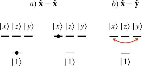
Figure 3: Graphical representation of the atomic internal variables (in the basis (11)) that can yield MQC signals upon demodulation, as explained in section 5, for (a) $\hat{\mathbf{x}}$-$\hat{\mathbf{x}}$ and (b) $\hat{\mathbf{x}}$-$\hat{\mathbf{y}}$ pump-probe polarization. (a) (black dots) populations $\langle\sigma_{11}\rangle$ (left) and $\langle\sigma_{xx}\rangle$ (right) of states $|1\rangle$ and $|x\rangle$, respectively, are modulated as $\cos(\varphi_{1}-\varphi_{2})$, (b) (red arc) Zeeman coherences $\langle\sigma_{xy}\rangle$ and $\langle\sigma_{yx}\rangle$ between the states $|x\rangle$ and $|y\rangle$ are modulated as $\exp(\pm\rmi(\varphi_{1}-\varphi_{2}))$.

Before we proceed, let us notice that, so far, we described the action of the laser pulses on the atoms non-perturbatively in the pulse area $\vartheta$. Strong pulses (e.g., $\vartheta\approx\pi$) induce a nonlinear response of the atoms  [19, 52] and can be used as a control and diagnostic tool in electronic spectroscopy [53, 54]. Furthermore, we have shown that strong pulses substantially modify the MQC signals [42]. However, in our present contribution we seek to elucidate the impact of the dipolar interactions on these signals. Thus, we adhere to the experimental conditions of [18] and evaluate (4.2.1) for small $\vartheta$, in the perturbative regime.

4.2.2 Beyond the ultrashort time scale.

We now derive from (23) the time evolution generated by the Liouvillian $\mathscr{L}_{\gamma}^{\alpha}$ as given by (14):

$$\dot{Q}_{\alpha}=\mathscr{L}_{\gamma}^{\alpha}Q_{\alpha},$$ (42)

with the formal solution (for simplicity, we take $t_{0}=0$)

$$Q_{\alpha}(t)=\exp\bigl{(}\mathscr{L}_{\gamma}^{\alpha}t\bigr{)}Q_{\alpha}(0).$$ (43)

The explicit solution is derived in A, with the result

$$Q_{\alpha}(t) = P_{\rme}Q_{\alpha}(0)P_{\mathrm{g}}\mathinner{\rme^{-\gamma t/2}}+P_{\mathrm{g}}Q_{\alpha}(0)P_{\rme}\mathinner{\rme^{-\gamma t/2}}$$ (44)

$$+P_{\mathrm{g}}Q_{\alpha}(0)P_{\mathrm{g}}+P_{\rme}Q_{\alpha}(0)P_{\rme}\mathinner{\rme^{-\gamma t}}+{\bf D}_{\alpha}^{\dagger}\cdot Q_{\alpha}(0){\bf D}_{\alpha}\left(1-\rme^{-\gamma t}\right),$$

where $P_{\rme}={\bf D}^{\dagger}_{\alpha}\cdot{\bf D}_{\alpha}$ is the projector on the subspace of excited states, and $P_{\mathrm{g}}=\mathbbm{1}-P_{\rme}$. Equation (44) has a transparent interpretation: the first line governs the exponential decay of electronic coherences with rate $\gamma/2$, while the remaining terms ensure trace conservation and the decay of excited state populations and Zeeman coherences with rate $\gamma$.

4.3 Dynamics of independent atoms: Multi-atom case

An arbitrary operator $Q(t)$ of $N$ atoms can now be obtained by combining single-atom operators $Q_{\alpha}$ in a tensor product, $Q(t)=\otimes_{\alpha=1}^{N}Q_{\alpha}(t)$. Consistently, the evolution of a composite operator $Q(t)$ in the case of non-interacting atoms is governed by superoperators

$$R_{j}^{\mathrm{L}}=\bigotimes_{\alpha=1}^{N}R^{\alpha}_{j},\quad\exp\left(\mathscr{L}_{\gamma}t\right)=\bigotimes_{\alpha=1}^{N}\exp\left(\mathscr{L}^{\alpha}_{\gamma}t\right),$$ (45)

where $\mathscr{L}_{\gamma}=\sum_{\alpha=1}^{N}\mathscr{L}_{\gamma}^{\alpha}$, the action of $R^{\alpha}_{j}$ is defined by equation (4.2.1), and that of $\mathscr{L}_{\gamma}^{\alpha}$ by (44). The superoperator $R^{\mathrm{L}}_{j}$ describes the coherent interaction of the individual atoms with the ultrashort incoming pulses, whereas $\exp(\mathscr{L}_{\gamma}t)$ governs their incoherent dynamics when the laser field is switched off.

We stress that, by (44), this dynamics amounts to an exponential decay of all atomic variables in the multi-atom excited state manifold (that is, all excited state populations, as well as Zeeman and electronic coherences), while the collective ground state of all atoms is unaffected by $\exp(\mathscr{L}_{\gamma}t)$.

Finally, we introduce the resolvent superoperator ${\cal G}_{\gamma}(z)$, $z\in\mathbb{C}$, which is the Laplace image of the evolution superoperator $\exp(\mathscr{L}_{\gamma}t)$,

$${\cal G}_{\gamma}(z)=\int_{0}^{\infty}\mathinner{\rmd t}\rme^{-zt}\rme^{\mathscr{L}_{\gamma}t}=\frac{1}{z-\mathscr{L}_{\gamma}},$$ (46)

and will be used in the next subsection, where we present the case of interacting atoms.

4.4 Dynamics of the dipole-dipole interacting atoms

4.4.1 Incorporation of $\mathscr{L}_{\rm int}$.

As discussed in section 4.1, the dipole-dipole interaction is relevant on short as well as on long time scales. Due to the weakness of the coupling parameter $|g(\xi)|$ in the far field (see section 3.4), the coupling $\mathscr{L}_{\rm int}$ can be readily included perturbatively into our solutions (45) for independent atoms. Note that this treatment is distinct from the traditional one [13, 17, 36, 37, 38], where the dipole-dipole interactions are accounted for non-perturbatively, via transformation to the exciton basis [19].

The starting point for the perturbative expansion in $\mathscr{L}_{\rm int}$ is the equation of motion for an $N$-atom operator $Q$, recall (12) and fig. 2,

$$\dot{Q}=\mathscr{L}_{\gamma}Q+\mathscr{L}_{\rm int}Q,$$ (47)

valid on short and long time scales. Solving (47) perturbatively in $\mathscr{L}_{\rm int}$, by the Laplace transform method [55], we obtain a series expansion

$$\tilde{Q}(z)=\sum_{n=0}^{\infty}{\cal G}_{\gamma}(z)\Bigl{[}\mathscr{L}_{\rm int}{\cal G}_{\gamma}(z)\Bigr{]}^{n}Q(t_{0}),$$ (48)

where $\tilde{Q}(z)=\int_{t_{0}}^{\infty}\mathinner{\rmd t^{\prime}}\exp(-zt^{\prime})Q(t^{\prime})$, and $Q(t_{0})$ is an operator which encodes the initial condition, to be specified below. The time evolution of $Q(t)$ then follows from (48) via the convolution theorem for Laplace transforms [55].

4.4.2 Combining piecewise solutions.

Equation (47) holds during the (short) interpulse delay $\tau$, and during the (long) fluorescence collection time $t_{\mathrm{fl}}$ (see figure 2). Therefore, when solving (47) with the aid of the Laplace transform, we introduce distinct variables for each interval, $z_{1}$ and $z_{2}$, respectively. During the short interpulse delay, the time evolution is given by the inverse Laplace transform

$$Q(\tau)=\frac{1}{2\pi\rmi}\int_{z_{0}-\rmi\infty}^{z_{0}+\rmi\infty}\mathinner{\rmd z_{1}}\rme^{z_{1}\tau}\tilde{Q}(z_{1}),$$ (49)

with $z_{0}\in\mathbb{R}$ chosen such that $z_{1}$ lies in the half-plane of convergence [55], and $\tilde{Q}(z_{1})$ is given by (48). The evolution during the long time interval is once again defined by (49), with the same $z_{0}$, and upon the replacements $z_{1}\rightarrow z_{2}$, $\tau\rightarrow t_{\rm fl}$.

The dynamics of the atomic operators during the ultrashort intervals can be absorbed in the Laplace transform solutions $\tilde{Q}(z_{1})$ and $\tilde{Q}(z_{2})$, through the initial conditions specified by $Q(t_{0})$ in (48). The short interval $\tau$ starts after the pump pulse at time $t_{1}$. Hence, by (31), we must set $Q(t_{0})\equiv Q(t_{1}^{+})=R_{1}^{\mathrm{L}}Q(t_{1}^{-})$ in (48), where $Q(t_{1}^{-})=Q(0)$, i.e., it describes atomic operators before any interaction took place. Likewise, for the long time interval starting after the probe pulse, we set $Q(t_{0})\equiv Q(t_{2}^{+})=R_{2}^{\mathrm{L}}Q(t_{2}^{-})$ in (48), with $Q(t_{2}^{-})$ given by the inverse Laplace transform (49) with $t_{2}^{-}=\tau$. Thus, through the initial conditions $Q(t_{2}^{+})$, a solution during the long time interval includes the action of two laser pulses and the evolution during the short time interval. Combination of piecewise solutions, each of which is valid on distinct time intervals, finally provides the evolution of an arbitrary atomic operator throughout the entire excitation-emission cycle.

4.4.3 Single and double scattering contributions.

The formal solution (48) applies for an arbitrary number $N$ of atoms, though we focus on the case $N=2$ in the following. At a first glance, this may appear a gross oversimplification of the experimentally studied physical system, including many atomic scatterers. Note, however, that we are dealing with a dilute thermal gas, whose fluorescence signal can be oftentimes inferred from the results for $N=1$ [16]. Yet, as we show below, one cannot measure a double quantum coherence signal by monitoring fluorescence of one, nor of two non-interacting atoms. Nor need we consider more than two atoms exchanging photons. Indeed, the atoms are in the far field of, and detuned from each other. The latter condition stems from the motion-induced Doppler shifts being much larger than the natural linewidth. The photon scattering mean free path [56] in such medium can be estimated as

$$\ell_{\rm sc}=\frac{1}{\rho\bar{\sigma}_{\mathrm{sc}}}\approx$88\text{\,}\mathrm{m}$,$$ (50)

with $\bar{\sigma}_{\mathrm{sc}}$ the mean scattering cross-section (see B). Therefore, a thermal atomic vapour of a reasonable size (say, a spherical cloud with a diameter $D$ of a few centimetres) is characterized by a very low optical thickness [40] $b=D/\ell_{\rm sc}\ll 1$, such that long scattering sequences of photons, mediating interactions between many particles, are highly improbable. Consistently, single and double scattering contributions do capture the essential physics in optically thin ensembles of scatterers [57], and we restrict our perturbative expansion (48) to second order in $\mathscr{L}_{\rm int}$. This is the lowest-order contribution which survives the disorder average, and it accounts for the double scattering of a single photon [26]. Thereby, we ignore recurrent scattering [58], where a photon bounces back and forth between the atoms, and which corresponds to a higher-order expansion in $\mathscr{L}_{\rm int}$. Neglecting such processes is fully justified in optically thin media [40].

Indeed, as we will see below, the above framework enables deducing 1QC and 2QC signals in good qualitative agreement with the experiment [18], and establishes the relevance of few-body systems in the characterization of MQC signals emitted by dilute thermal atomic ensembles.

The single and double scattering contributions can be derived from the two-dimensional Laplace transforms

$$\tilde{Q}^{[n]}(z_{1},z_{2},\varphi_{1},\varphi_{2}) = \sum_{p=0}^{n}{\cal G}_{\gamma}(z_{2})\Bigl{[}\mathscr{L}_{\rm int}{\cal G}_{\gamma}(z_{2})\Bigr{]}^{n-p}$$ (51)

$$\qquad\times\mathinner{R_{2}^{\mathrm{L}}}{\cal G}_{\gamma}(z_{1})\Bigl{[}\mathscr{L}_{\rm int}{\cal G}_{\gamma}(z_{1})\Bigr{]}^{p}\mathinner{R_{1}^{\mathrm{L}}}Q(0),$$

with $n=0,2$, which are obtained from equation (48) and the contribution of piecewise solutions as described in section 4.4.2. Note that the phase tags (from equation (30)) in the argument of (51) are absorbed in $R_{1}^{\mathrm{L}}$ and $R_{2}^{\mathrm{L}}$, via (36) and (45).

To infer the detected fluorescence intensity from the operator equation (51), we need specific atomic correlation functions which correspond to $\alpha=\beta$ in equation (10) (see section 4.1). These are obtained by representing the operator equations in matrix form, via the complete basis of the operator space for two atoms (see C), and subsequently evaluating the quantum mechanical expectation value, followed by the configuration average:

$$\left\langle\langle\tilde{\bf Q}^{[n]}(z_{1},z_{2},\varphi_{1},\varphi_{2})\rangle\right\rangle_{\rm conf} = \sum_{p=0}^{n}\Bigl{\langle}{\bf G}_{\gamma}(z_{2})\Bigl{[}{\bf V}{\bf G}_{\gamma}(z_{2})\Bigr{]}^{n-p}$$ (52)

$$\times{\bf R}_{2}^{\mathrm{L}}{\bf G}_{\gamma}(z_{1})\Bigl{[}{\bf V}{\bf G}_{\gamma}(z_{1})\Bigr{]}^{p}{\bf R}_{1}^{\mathrm{L}}\langle{\bf Q}(0)\rangle\Bigr{\rangle}_{\mathrm{conf}},$$

where ${\bf G}_{\gamma}(z)$, ${\bf R}_{j}^{\mathrm{L}}$, and ${\bf V}$ are $256\times 256$ matrices representing operators ${\cal G}_{\gamma}(z)$, and $R^{\mathrm{L}}_{j}$, ${\cal L}_{\rm int}$, respectively, with elements given by

$$[{\bf G}_{\gamma}(z)]_{kl}=\mathop{\mathrm{Tr}}\left\{Q_{l}^{\dagger}{\cal G}_{\gamma}Q_{k}\right\},\,[{\bf R}_{j}^{\mathrm{L}}]_{kl}=\mathop{\mathrm{Tr}}\left\{Q_{l}^{\dagger}R_{j}^{\mathrm{L}}Q_{k}\right\},\,[{\bf V}]_{kl}=\mathop{\mathrm{Tr}}\left\{Q_{l}^{\dagger}\mathscr{L}_{\rm int}Q_{k}\right\},$$

while $[{\bf Q}(0)]_{k}=\mathop{\mathrm{Tr}}\left\{Q^{\dagger}_{k}|1\rangle_{1}\langle 1|_{1}\otimes|1\rangle_{2}\langle 1|_{2}\right\}$ is a vector with 256 elements. Let us finally represent the Liouvillians $\mathscr{L}_{\rm int}^{(1)}$ and $\mathscr{L}_{\rm int}^{(2)}$, see (21) and (22), with the matrices

$$[{\bf V}^{(1)}]_{kl}=\mathop{\mathrm{Tr}}\left\{Q_{l}^{\dagger}\mathscr{L}^{(1)}_{\rm int}Q_{k}\right\},\quad[{\bf V}^{(2)}]_{kl}=\mathop{\mathrm{Tr}}\left\{Q_{l}^{\dagger}\mathscr{L}^{(2)}_{\rm int}Q_{k}\right\}.$$ (53)

4.4.4 Configurational average.

The configuration or disorder average in (52) is necessary to capture the impact of changes of the random atomic configuration during the fluorescence detection (section 4.1). As a result of averaging, all terms carrying position-dependent phases vanish. In addition to interference contributions with $\alpha\neq\beta$ in equation (10) which are already excluded in (52), the disorder average obliterates all terms with ${\bf r}_{\alpha 0}$–dependent phases—which are due to the action of the two incoming laser pulses (see equations (30), (36)). What remains are terms carrying position-independent phases that originate in single scattering processes, independent of ${\bf V}$, and double scattering processes, quadratic in ${\bf V}$. These single and double scattering contributions have weights $|g(\bar{\xi})|^{0}=1$ and $|g(\bar{\xi})|^{2}=1/\bar{\xi}^{2}$, respectively.

Furthermore, only particular products of the matrix elements of $\overset{\text{\tiny$\bm{\leftrightarrow}$}}{\mathbf{T}}(\bar{\xi},\hat{\mathbf{n}})$ (which enter (52) at second order in $\mathscr{L}_{\rm int}$, through (16)) contribute to the average signal upon integration over the isotropic distribution of the vector $\hat{\mathbf{n}}$ [25, 26]: $\langle\overset{\text{\tiny$\bm{\leftrightarrow}$}}{\mathbf{T}}_{kl}\overset{\text{\tiny$\bm{\leftrightarrow}$}}{\mathbf{T}}{}^{*}_{mn}\rangle_{\mathrm{conf}}\neq 0$ if and only if the indices $k,l,m,n$ are pairwise identical, cf. D. This amounts to the suppression, in the average fluorescence intensity, of all contributions stemming from the interference of atomic excited state sublevels with different magnetic quantum numbers.

Finally, note that through the matrix ${\bf R}^{\mathrm{L}}_{j}$ the atomic correlation functions carry phases $\Delta_{\alpha}t_{j}$ proportional to the Doppler shifts, by virtue of (30), (36). Unlike the uniform spatial distribution of the atoms, the Doppler shifts $\Delta_{\alpha}$ are non-uniformly Maxwell-Boltzmann distributed. Therefore, the result of averaging over $\Delta_{\alpha}$ is different from that of averaging over random atomic positions; it would not eliminate the terms including velocity-dependent phases, but instead result in inhomogeneous line broadening [31] of MQC spectra [42]. In our present contribution, we ignore this effect and set the Doppler shifts in equation (30) to zero, while focusing on the general structure and physical origin of the resonances of 1QC and 2QC spectra.

The final result after configuration averaging is a number of terms which contribute to the single and double scattering intensities. More precisely, these terms, derived from the vectors $\langle\langle\tilde{\bf Q}^{[0]}(z_{1},z_{2},\varphi_{1},\varphi_{2})\rangle\rangle_{\mathrm{conf}}$ and $\langle\langle\tilde{\bf Q}^{[2]}(z_{1},z_{2},\varphi_{1},\varphi_{2})\rangle\rangle_{\mathrm{conf}}$ in equation (52), yield the two-dimensional Laplace images of the single and double scattering transient intensities denoted, respectively, by $\tilde{I}^{[0]}_{\hat{\mathbf{k}}}(z_{1},z_{2},\varphi_{1},\varphi_{2})$ and $\tilde{I}^{[2]}_{\hat{\mathbf{k}}}(z_{1},z_{2},\varphi_{1},\varphi_{2})$.

We can draw general conclusions about the dependence of $\tilde{I}^{[0]}_{\hat{\mathbf{k}}}(z_{1},z_{2},\varphi_{1},\varphi_{2})$ and $\tilde{I}^{[2]}_{\hat{\mathbf{k}}}(z_{1},z_{2},\varphi_{1},\varphi_{2})$ on the phases $\varphi_{j}$. This is possible because, by (30), the $\varphi_{j}$ ($j=1,2$) are linear functions on the random initial positions ${\bf r}_{0\alpha}$ of the first or second atom, that is $\varphi_{j}=\varphi_{j\alpha}$ ($\alpha=1,2$). Consequently, the average functions $\tilde{I}^{[n]}_{\hat{\mathbf{k}}}(z_{1},z_{2},\varphi_{1},\varphi_{2})$ ($n=0,2$) vanish unless they depend solely on a phase factor proportional to the difference $\varphi_{21}=\varphi_{2\alpha}-\varphi_{1\alpha}=\omega_{0}\tau+w_{21}\tau_{m}$ or, trivially, are independent of $\varphi_{j\alpha}$. More explicitly, the non-vanishing intensities $\tilde{I}^{[n]}_{\hat{\mathbf{k}}}(z_{1},z_{2},\varphi_{1},\varphi_{2})=\tilde{I}^{[n]}_{\hat{\mathbf{k}}}(z_{1},z_{2},\varphi_{21})$ can then be written as

$$\tilde{I}^{[0]}_{\hat{\mathbf{k}}}(z_{1},z_{2},\varphi_{21}) = \sum_{l=-1}^{1}\tilde{I}^{[0]}_{l,\hat{\mathbf{k}}}(z_{1},z_{2})\rme^{\rmi\varphi_{21}l},$$ (54)

$$\tilde{I}^{[2]}_{\hat{\mathbf{k}}}(z_{1},z_{2},\varphi_{21}) = \sum_{l=-2}^{2}\tilde{I}^{[2]}_{l,\hat{\mathbf{k}}}(z_{1},z_{2})\rme^{\rmi\varphi_{21}l}.$$ (55)

The summation range in (54) is a consequence of equation (39): since, for $n=0$, the time evolution (52) is local in the Hilbert space of each atom, individual atomic operators can depend only on the phase tags $\rme^{\pm\rmi\varphi_{21}}$, and not on $\rme^{\pm 2\rmi\varphi_{21}}$. In contrast, fluorescence intensity emerging due to double scattering can carry phases $\pm 2\varphi_{21}$ in $\tilde{I}^{[2]}_{\hat{\mathbf{k}}}(z_{1},z_{2},\varphi_{21})$, giving rise to 2QC signals.

Taking the inverse Laplace transforms (see (49)) of the functions defined by (54) and (55) with respect to $z_{1}$ and $z_{2}$, we obtain the associated time-domain expressions $I^{[0]}_{l,\hat{\mathbf{k}}}(\tau,t_{\rm fl},\varphi_{21})$ and $I^{[2]}_{l,\hat{\mathbf{k}}}(\tau,t_{\rm fl},\varphi_{21})$,

$$I^{[0]}_{\hat{\mathbf{k}}}(\tau,t_{\rm fl},\varphi_{21}) = \sum_{l=-1}^{1}I^{[0]}_{l,\hat{\mathbf{k}}}(\tau,t_{\rm fl})\rme^{\rmi\varphi_{21}l},$$ (56)

$$I^{[2]}_{\hat{\mathbf{k}}}(\tau,t_{\rm fl},\varphi_{21}) = \sum_{l=-2}^{2}I^{[2]}_{l,\hat{\mathbf{k}}}(\tau,t_{\rm fl})\rme^{\rmi\varphi_{21}l},$$ (57)

where $I^{[0]}_{l,\hat{\mathbf{k}}}(\tau,t_{\rm fl})$ and $I^{[2]}_{l,\hat{\mathbf{k}}}(\tau,t_{\rm fl})$ are exponentially decaying functions of $\tau$ and $t_{\rm fl}$ (recall our discussion in section 4.3), related to $\tilde{I}^{[n]}_{l,\hat{\mathbf{k}}}(z_{1},z_{2})$ by the two-dimensional Laplace transform:

$$\tilde{I}^{[n]}_{l,\hat{\mathbf{k}}}(z_{1},z_{2})=\int_{0}^{\infty}\mathinner{\rmd\tau}\rme^{-z_{1}\tau}\int_{0}^{\infty}\mathinner{\rmd t_{\rm fl}}\rme^{-z_{2}t_{\rm fl}}I^{[n]}_{l,\hat{\mathbf{k}}}(\tau,t_{\rm fl}).$$ (58)

The total transient intensity is the sum of (56) and (57),

$$I_{\hat{\mathbf{k}}}(\tau,t_{\rm fl},\varphi_{21})=I^{[0]}_{\hat{\mathbf{k}}}(\tau,t_{\rm fl},\varphi_{21})+I^{[2]}_{\hat{\mathbf{k}}}(\tau,t_{\rm fl},\varphi_{21}),$$ (59)

which can be used to deduce 1QC and 2QC spectra, as outlined in section 2, and discussed below.

4.4.5 Signal demodulation.

The goal of the demodulation procedure is to extract only those specific components from the fluorescence signal, which oscillate at defined integer multiples $\kappa$ of the modulation frequency $w_{21}$. The spectra of these signals, generally referred to as multiple quantum coherences (MQC), are extracted from (2), after replacement of $\phi_{1}$ and $\phi_{2}$ by the phase difference $\varphi_{21}$, via the following two-fold, half-sided Fourier transforms,

$$S_{\hat{\mathbf{k}}}(\omega;\kappa) = \lim_{\mathscr{F}\to 0}\frac{\mathscr{F}}{\sqrt{2\pi}}\int_{0}^{\infty}\mathinner{\rmd\tau}_{m}\rme^{-(\mathscr{F}+\rmi\kappa w_{21})\tau_{m}}\int_{0}^{\infty}\mathinner{\rmd\tau}\rme^{-\rmi\omega\tau}$$ (60)

$$\times\int_{0}^{\infty}\mathinner{\rmd t_{\rm fl}}I_{\hat{\mathbf{k}}}(\tau,t_{\rm fl},\varphi_{21}),$$

with $\kappa=1,2$ the MQC orders here considered. (59), with $I^{[0]}_{\hat{\mathbf{k}}}(\tau,t_{\mathrm{fl}},\varphi_{21})$ and $I^{[2]}_{\hat{\mathbf{k}}}(\tau,t_{\mathrm{fl}},\varphi_{21})$ from (56) and (57), into (60), and integration over $\tau_{m}$ yields the result:

$$S_{\hat{\mathbf{k}}}(\omega;\kappa) = \lim_{\mathscr{F}\to 0}\frac{\mathscr{F}}{\sqrt{2\pi}}\left[\sum_{l=-1}^{1}\int_{0}^{\infty}\mathinner{\rmd\tau}\rme^{-\rmi(\omega-l\omega_{0})\tau}\int_{0}^{\infty}\mathinner{\rmd t_{\mathrm{fl}}}\frac{I^{[0]}_{l,\hat{\mathbf{k}}}(\tau,t_{\mathrm{fl}})}{\mathscr{F}+\rmi(\kappa-l)w_{21}}\right.$$ (61)

$$\left.+\sum_{l=-2}^{2}\int_{0}^{\infty}\mathinner{\rmd\tau}\rme^{-\rmi(\omega-l\omega_{0})\tau}\int_{0}^{\infty}\mathinner{\rmd t_{\mathrm{fl}}}\frac{I^{[2]}_{l,\hat{\mathbf{k}}}(\tau,t_{\mathrm{fl}})}{\mathscr{F}+\rmi(\kappa-l)w_{21}}\right].$$

The limit ${\cal F}\to 0$ selects only terms corresponding to $l=\kappa$ in (61), and is equivalent to (58) evaluated at $z_{1}=\rmi(\omega-\kappa\omega_{0})$ and $z_{2}=0$. We thus arrive at the final expressions for the 1QC and 2QC spectra, which exhibit resonances at $\omega=\omega_{0}$ and $\omega=2\omega_{0}$, respectively:

$$S_{\hat{\mathbf{k}}}(\omega;1) = \frac{1}{\sqrt{2\pi}}\tilde{I}^{[0]}_{1,\hat{\mathbf{k}}}(\rmi\bigl{(}\omega-\omega_{0}),0\bigr{)}+\frac{1}{\sqrt{2\pi}}\tilde{I}^{[2]}_{1,\hat{\mathbf{k}}}\bigl{(}\rmi(\omega-\omega_{0}),0\bigr{)},$$ (62)

$$S_{\hat{\mathbf{k}}}(\omega;2) = \frac{1}{\sqrt{2\pi}}\tilde{I}^{[2]}_{2,\hat{\mathbf{k}}}\bigl{(}\rmi(\omega-2\omega_{0}),0\bigr{)}.$$ (63)

To summarise, through (62) and (63) we connect 1QC and 2QC spectra as measured by methods of phase-modulated spectroscopy to specific components of the fluorescence intensity emitted by two atoms. The intensity is expressed via (10) (with $N=2$ and, as a consequence of the configuration average over the atomic random positions, $\alpha=\beta$) through the excited state populations of single atoms that may be independent or interacting with each other by exchanging a single photon. Furthermore, while equation (62) indicates that the 1QC signal is fed by both, single and double scattering processes, equation (63) shows that 2QC signal can stem solely from double scattering, see figure 4. In other words, whereas 1QC signals may be observed on independent particles, 2QC signals are always an unambiguous proof of interatomic interactions. Thus the origin of 2QC signals in phase-modulated spectroscopy on disordered samples [15, 18] is substantially different from the one outlined in [16], where 2QC signals stem from two-atom observables of non-interacting atoms.

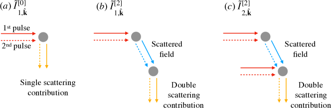
Figure 4: Diagrammatic representation of single (a) and double (b,c) scattering processes contributing to intensities $\tilde{I}^{[0]}_{1,\hat{\mathbf{k}}}$, $\tilde{I}^{[2]}_{1,\hat{\mathbf{k}}}$, and $\tilde{I}^{[2]}_{2,\hat{\mathbf{k}}}$, respectively (see (62), (63)). Horizontal red lines indicate the incoming laser pulses, vertical yellow lines the emitted fluorescence, oblique blue lines the scattered fields via dipole-dipole interactions. Solid and dashed lines indicate single field amplitudes and their complex conjugates (see also figure 1). The difference between the double scattering processes (b) and (c) is that, in the former case, fluorescence stems from the excited state sublevels of the second atom that are driven by the scattered, but not by the incident field, while, in the latter case, by both the scattered and the incident field. As discussed in section 5, processes (a,b) and (c) are associated with 1QC and 2QC signals, respectively.

The dipolar interactions are represented by excitation exchange and collective decay processes encapsulated in the Liouvillians ${\cal L}_{\alpha\beta}^{(1)}$ and ${\cal L}_{\alpha\beta}^{(2)}$ defined by (21) and (22). In section 5, we present the spectra (62) and (63) and elucidate the significance of these Liouvillians for the emergence of 1QC and 2QC signals, which explains a number of experimentally observed features of MQC spectra [18].

5 Spectra of single and double quantum coherence signals

In figure 5 we plot the single and double coherence spectra $S_{\hat{\mathbf{k}}}(\omega;1)$ and $S_{\hat{\mathbf{k}}}(\omega;2)$, given by (62) and (63), for $\hat{\mathbf{k}}=\hat{\mathbf{x}},\hat{\mathbf{y}}$, and for parallel ($\hat{\mathbf{x}}$-$\hat{\mathbf{x}}$) and perpendicular ($\hat{\mathbf{x}}$-$\hat{\mathbf{y}}$) pump-probe polarization channels (in brief, $\parallel$ and $\perp$ channels). As discussed in section 4.4.4, these signals emerge from the configuration average. For illustration, the background of each panel in figure 5 shows MQC spectra stemming from pairs of atoms at fixed locations. These were calculated by omitting the average $\langle\ldots\rangle_{\mathrm{conf}}$ in (52) and, instead, by considering randomly drawn configurations $(\xi,\hat{\mathbf{n}})$, which determine the tensor $\overset{\text{\tiny$\bm{\leftrightarrow}$}}{\mathbf{T}}$ and the phase factor $\exp(\rmi{\bf k}\cdot{\bf r}_{12})$—as detailed in the caption of figure 5. The deviations between background and averaged spectra are striking for both parallel and perpendicular pulses: the single realizations have little resemblance with the true (configuration averaged) line shapes, from which they oftentimes differ by orders of magnitude. The absence of the configuration average constitutes one of several reasons for a substantial qualitative and quantitative mismatch between the model including two fixed molecules [17] and the observations reported in [18]. Further reasons will be identified below. Henceforth, we will discuss our configuration-averaged spectra.

We stress that, while our general analytical solutions, derived from (51) and (52), assume that dipolar interactions act during both, the interpulse delay and fluorescence harvesting, we have checked numerically that the 1QC and 2QC spectra can be fully understood if we include the interatomic interactions only during the fluorescence detection stage. This is reasonable, given the typically short duration of $\sim$10\text{\,}\mathrm{ps}$$ of the interpulse delay and the weakness of the dipolar coupling. Therefore, throughout this section we interpret the emergence of 2QC spectra (as much as contributions to 1QC spectra) as the result of dipole-dipole interactions during the long time scale, i.e. after the atoms have interacted with the two incoming laser pulses.

In the $\parallel$ channel, the real and imaginary parts of the 1QC spectra exhibit, respectively, absorptive and dispersive resonances at $\omega=\omega_{0}$. In the here realized regime of relatively weak (perturbative) driving fields, these line shapes are consistently proportional to the real and imaginary parts of the linear susceptibility [29]. For both choices of pump-probe polarizations and observation directions, the 2QC spectra feature qualitatively identical line shapes centred at $\omega=2\omega_{0}$, albeit with opposite sign to the 1QC spectra. The sign flip of the 2QC spectra can be understood by recalling that they originate from double scattering. Thereby, each atom effectively interacts with four fields: two laser pulses and two far-fields scattered by the other atom, see figure 4 (c). This nonlinear four-wave mixing process is described by the third-order susceptibility [19, 59], whose sign is opposite to that of the linear susceptibility [59]. We would like to stress that the sign flip of the 2QC spectra was experimentally observed [28], but its interpretation has been lacking.

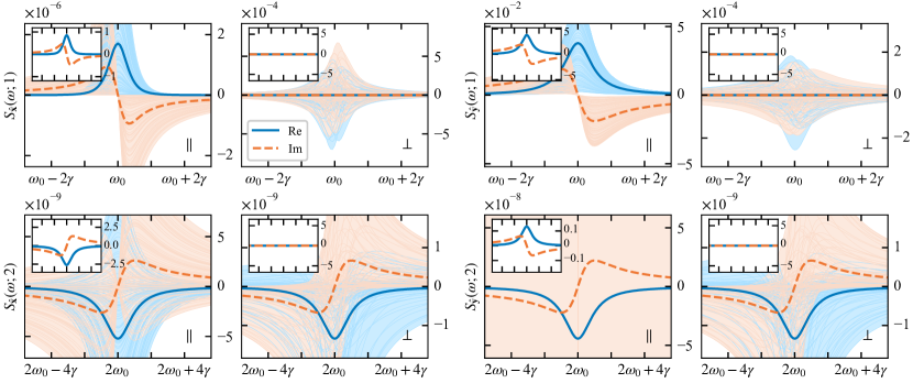
Figure 5: Real (solid lines) and imaginary (dashed lines) parts of the MQC spectra $S_{\hat{\mathbf{k}}}(\omega;\kappa)$ [in units of spectral density integrated over the fluorescence detection time, $f^{2}/\gamma^{2}$; see (10) and (60)], for detection directions $\hat{\mathbf{k}}=\hat{\mathbf{x}}$ (left) and $\hat{\mathbf{k}}=\hat{\mathbf{y}}$ (right), and for quantum coherences of order $\kappa=1$ (top) and $\kappa=2$ (bottom). Symbols $\parallel$ and $\perp$ indicate parallel ($\hat{\mathbf{x}}$-$\hat{\mathbf{x}}$) and perpendicular ($\hat{\mathbf{x}}$-$\hat{\mathbf{y}}$) pump-probe polarizations, respectively. Parameter values match the experimental ones [18]: average interatomic distance $\bar{r}\approx$10\text{\,}\mathrm{\SIUnitSymbolMicro m}$$ (which corresponds to a particle density $\rho=${10}^{8}\text{\,}{\mathrm{cm}}^{-3}$$), laser pulse areas $\vartheta=$0.14$\pi$ and durations $\sigma=$21\text{\,}\mathrm{f}\mathrm{s}$$ (tuned to resonance with the D2-line of ⁸⁷Rb atoms [30]), transition wavelength $\lambda_{0}=$790\text{\,}\mathrm{n}\mathrm{m}$$, and spontaneous decay rate $\gamma\approx 2\pi\times$6.067\text{\,}\mathrm{M}\mathrm{H}\mathrm{z}$$. This choice of parameters results in a mean scaled interatomic distance $\bar{\xi}=k_{0}\bar{r}\approx 80$, with $k_{0}$ the atomic transition’s wave number. Thin lines in the background show MQC spectra (with the same color coding for the real and imaginary parts as the average spectra) for 100 random configurations $(\xi,\hat{\bf n})$, with $\xi$ distributed uniformly in the interval $67.2<\xi<92.8$, and $\hat{\bf n}$ distributed isotropically. The insets show the signals obtained by substituting $\overset{\text{\tiny$\bm{\leftrightarrow}$}}{\mathbf{T}}\mapsto\rmi\overset{\text{\tiny$\bm{\leftrightarrow}$}}{\mathbf{\Omega}}$, which amounts to ignoring the collective decay processes.

In the $\parallel$ channel, the peak magnitude of the 1QC signal for $\hat{\mathbf{k}}=\hat{\mathbf{x}}$ is four orders of magnitude smaller than for $\hat{\mathbf{k}}=\hat{\mathbf{y}}$, see figure 5. This significant difference arises because the signal for $\hat{\mathbf{k}}=\hat{\mathbf{y}}$ is dominated by single scattering from individual atoms, as illustrated by figure 4 (a) (i.e., by the $\tilde{I}^{[0]}_{1,\hat{\mathbf{k}}}$ component in (62)). This contribution to the single coherence signal is independent of the interatomic distance. For $\hat{\mathbf{k}}=\hat{\mathbf{x}}$, on the contrary, the atoms in their $|x\rangle$ state cannot directly emit in the $\hat{\bf x}$-direction. Hence, the signal is due to double scattering contribution $\tilde{I}^{[2]}_{1,\hat{\mathbf{k}}}$ (see figure 4 (b)), wherein the excitation is transferred from the state $|x\rangle$ of one atom to the state $|y\rangle$ or $|z\rangle$ of the other — which was in its ground state prior to the interaction. Such an interaction process, involving the exchange of an excitation between the atoms, is mediated solely by the Liouvillian ${\cal L}_{\alpha\beta}^{(1)}$, see (21). The total average probability of this process is proportional to $\langle\overset{\text{\tiny$\bm{\leftrightarrow}$}}{\mathbf{T}}_{xr}\overset{\text{\tiny$\bm{\leftrightarrow}$}}{\mathbf{T}}{}^{*}_{xr}\rangle_{\mathrm{conf}}=\langle\overset{\text{\tiny$\bm{\leftrightarrow}$}}{\mathbf{\Omega}}_{xr}\overset{\text{\tiny$\bm{\leftrightarrow}$}}{\mathbf{\Omega}}_{xr}\rangle_{\mathrm{conf}}+\langle\overset{\text{\tiny$\bm{\leftrightarrow}$}}{\mathbf{\Gamma}}_{xr}\overset{\text{\tiny$\bm{\leftrightarrow}$}}{\mathbf{\Gamma}}_{xr}\rangle_{\mathrm{conf}}$ ($r=y,z$), which yields a nonzero contribution $\sim 1/\bar{\xi}^{2}=0.00016$ for $\bar{\xi}=80$ (see caption of figure 5), justifying the difference, by four orders of magnitude, between the 1QC signals in the $\hat{\mathbf{x}}$ and $\hat{\mathbf{y}}$ directions.

Note the complete absence in our data of the 1QC signal in the $\perp$ channel (see 2^nd and 4^th panel in the top row of figure 5), corroborating the experiment [18]. This is due to orthogonally polarized laser pulses imprinting the correct phase for demodulation only on the Zeeman coherences (see section 4.2.1), i.e. the off-diagonal elements $\langle\sigma_{xy}^{\alpha}\rangle$ in the excited state manifold of the atomic density matrix, which do not directly fluoresce. While the dipole-dipole interaction can transfer the Zeeman coherence of atom $\alpha$ to the excited state population $\langle\sigma_{rr}^{\beta}\rangle$ ($r\in\{x,y,z\}$) of the initially unexcited atom $\beta$ via the matrix ${\bf V}^{(1)}$ (see section 3.4 and equation (53)), the probability of this process is proportional to $\overset{\text{\tiny$\bm{\leftrightarrow}$}}{\mathbf{T}}_{xr}\overset{\text{\tiny$\bm{\leftrightarrow}$}}{\mathbf{T}}{}^{*}_{yr}$, which vanishes upon disorder averaging (see section 4.4.4 and D). It must be emphasized that an appropriate assessment of MQC signals in the $\perp$ channel is only possible when the vector character of light fields and dipoles is accounted for, and is therefore out of reach for scalar atom models  [13, 16, 17, 36, 37, 60].

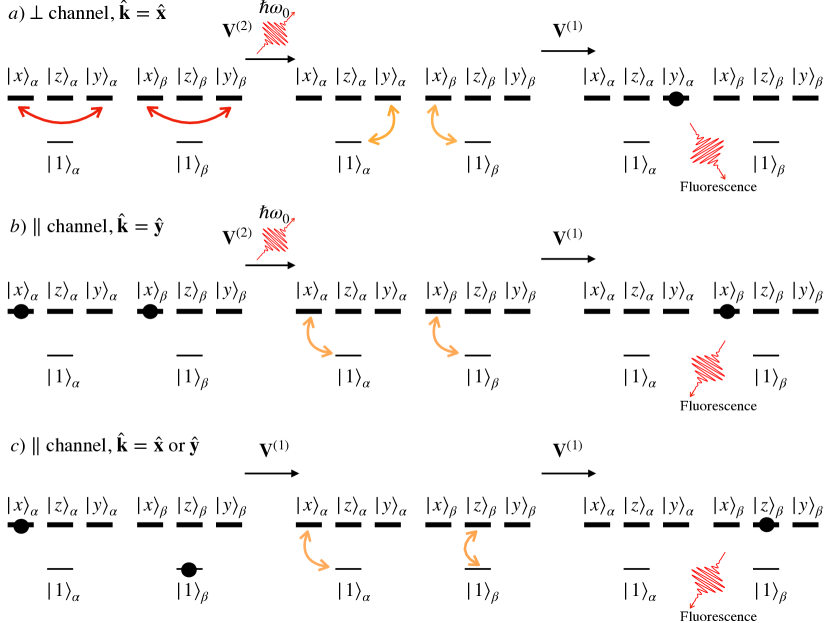
Figure 6: Excitation pathways describing the transformation of the initial two-atom variables with the correct phase for demodulation of 2QC signals (see section 4.2.1 and figure 3) to the excited state populations of the atoms which give rise to fluorescence signals. Only those variables that contribute to 2QC signals are indicated. (a) In the $\perp$ channel and for the observation direction $\hat{\mathbf{k}}=\hat{\mathbf{x}}$, Zeeman coherences $\langle\sigma_{xy}^{\alpha}\rangle\langle\sigma_{xy}^{\beta}\rangle$ (red arcs) of independent atoms are transformed, by the collective decay process mediated by the matrix ${\bf V}^{(2)}$, and accompanied by the emission of a single photon, into electronic coherences (orange arcs), e.g., $\langle\sigma^{\alpha}_{1y}\sigma^{\beta}_{x1}\rangle$. By the interaction represented by the matrix ${\bf V}^{(1)}$, the atomic state $|y\rangle_{\alpha}$ is excited, while atom $\beta$ is de-excited, which is described by the correlator $\langle\sigma^{\alpha}_{yy}\sigma^{\beta}_{11}\rangle$ (black dot). The fluorescence emitted by atom $\alpha$ contributes to the 2QC signal. (b) In the $\parallel$ channel and for the observation direction $\hat{\mathbf{k}}=\hat{\mathbf{y}}$, the pathway indicates the following sequence of processes: $\langle\sigma^{\alpha}_{xx}\rangle\langle\sigma^{\beta}_{xx}\rangle\overset{{\bf V}^{(2)}}\longrightarrow\langle\sigma^{\alpha}_{1x}\sigma^{\beta}_{x1}\rangle\overset{{\bf V}^{(1)}}\longrightarrow\langle\sigma^{\alpha}_{11}\sigma^{\beta}_{xx}\rangle$. (c) In the $\parallel$ channel and for the observation directions $\hat{\mathbf{k}}=\hat{\mathbf{y}}$ or $\hat{\mathbf{x}}$, additional pathways are mediated solely by the matrices ${\bf V}^{(1)}$: $\langle\sigma^{\alpha}_{xx}\rangle\langle\sigma^{\beta}_{11}\rangle\overset{{\bf V}^{(1)}}\longrightarrow\langle\sigma^{\alpha}_{1x}\sigma^{\beta}_{z1}\rangle\overset{{\bf V}^{(1)}}\longrightarrow\langle\sigma^{\alpha}_{11}\sigma^{\beta}_{zz}\rangle$.

In the same ($\perp$) pump-probe configuration, 2QC signals are however present – in qualitative agreement with experiment [18]. They originate from the Zeeman coherences $\langle\sigma_{xy}^{\alpha}\sigma_{xy}^{\beta}\rangle=\langle\sigma_{xy}^{\alpha}\rangle\langle\sigma_{xy}^{\beta}\rangle$ (as discussed above, this two-atom correlation function factorizes because the atoms have not yet interacted with each other) induced by the incoming pulses in both atoms (recall our discussion in section 4.2.1 accompanying figure 3(b)). Given such a doubly-excited state, the matrix ${\bf V}^{(2)}$ (see equation (53)) mediates a collective decay process (see figure 6 (a)), where one photon is emitted by both atoms, transforming the initial two-atom product state with Zeeman coherences into a mixed (possibly entangled) state exhibiting electronic coherences of the atoms, e.g. $\langle\sigma^{\alpha}_{1y}\sigma^{\beta}_{x1}\rangle$. This process is linear in $\overset{\text{\tiny$\bm{\leftrightarrow}$}}{\mathbf{\Gamma}}_{xy}$ and, hence, does not directly contribute to the average 2QC signal. However, the electronic coherence of one atom can be further transformed via the matrix ${\bf V}^{(1)}$ into the excited state population of the other atom, such as $\langle\sigma^{\alpha}_{11}\sigma^{\beta}_{xx}\rangle$ or $\langle\sigma^{\alpha}_{yy}\sigma^{\beta}_{11}\rangle$ (see figure 6 (a)). Although ${\bf V}^{(1)}$ is linear in both $\overset{\text{\tiny$\bm{\leftrightarrow}$}}{\mathbf{\Omega}}$ and $\overset{\text{\tiny$\bm{\leftrightarrow}$}}{\mathbf{\Gamma}}$, the total average probability of preparing such a state is proportional to $\langle\overset{\text{\tiny$\bm{\leftrightarrow}$}}{\mathbf{\Gamma}}_{yx}\overset{\text{\tiny$\bm{\leftrightarrow}$}}{\mathbf{\Gamma}}_{xy}\rangle_{\mathrm{conf}}\neq 0$ (while $\langle\overset{\text{\tiny$\bm{\leftrightarrow}$}}{\mathbf{\Gamma}}_{yx}\overset{\text{\tiny$\bm{\leftrightarrow}$}}{\mathbf{\Omega}}_{xy}\rangle_{\mathrm{conf}}=0$, cf. D). Subsequent fluorescence from such a state, consisting of one atom in the excited and the other one in the ground state, does give rise to a non-vanishing average 2QC signal with the same intensity in directions $\hat{\bf y}$ and $\hat{\bf x}$, respectively.

In the $\parallel$ channel, the correct phase for demodulation of 2QC signals is carried by combinations of the two-atom correlators $\langle\sigma_{xx}^{\alpha}\sigma_{xx}^{\beta}\rangle=\langle\sigma_{xx}^{\alpha}\rangle\langle\sigma_{xx}^{\beta}\rangle$, $\langle\sigma_{11}^{\alpha}\sigma_{xx}^{\beta}\rangle=\langle\sigma_{11}^{\alpha}\rangle\langle\sigma_{xx}^{\beta}\rangle$, and $\langle\sigma_{xx}^{\alpha}\sigma_{11}^{\beta}\rangle=\langle\sigma_{xx}^{\alpha}\rangle\langle\sigma_{11}^{\beta}\rangle$ (see section 4.2.1). A possible pathway that can lead to the contribution of the correlator $\langle\sigma_{xx}^{\alpha}\sigma_{xx}^{\beta}\rangle$ to the fluorescence signal in direction $\hat{\mathbf{y}}$ is the following: By means of two interactions generated by the matrices ${\bf V}^{(2)}$ and ${\bf V}^{(1)}$ (see figure 6 (b)), one atom is prepared in the ground and the other in the excited state $|x\rangle$. This is analogous to how the Zeeman coherences $\langle\sigma_{xy}^{\alpha}\sigma_{xy}^{\beta}\rangle$ can contribute to the signal in the $\perp$ channel. The total average probability of preparing such state is $\propto\langle\overset{\text{\tiny$\bm{\leftrightarrow}$}}{\mathbf{\Gamma}}_{xx}\overset{\text{\tiny$\bm{\leftrightarrow}$}}{\mathbf{\Gamma}}_{xx}\rangle_{\mathrm{conf}}$, and a 2QC signal due to the correlator $\langle\sigma_{11}^{\alpha}\sigma_{xx}^{\beta}\rangle$ can be observed in direction $\hat{\bf y}$. The correlation functions $\langle\sigma_{11}^{\alpha}\sigma_{xx}^{\beta}\rangle$ and $\langle\sigma_{xx}^{\alpha}\sigma_{11}^{\beta}\rangle$, instead, can contribute to 2QC spectra via two interactions generated by the matrix ${\bf V}^{(1)}$ (for the correlation function $\langle\sigma_{xx}^{\alpha}\rangle\langle\sigma_{11}^{\beta}\rangle$, a possible pathway is displayed in figure 6 (c)). Excited state populations are thereby transferred from atom $\alpha$ to atom $\beta$ or vice versa (figure 6 (c) shows a pathway leading to the correlator $\langle\sigma_{11}^{\alpha}\sigma_{zz}^{\beta}\rangle$). The total average probability of such processes is $\propto\langle\overset{\text{\tiny$\bm{\leftrightarrow}$}}{\mathbf{\Gamma}}_{xr}\overset{\text{\tiny$\bm{\leftrightarrow}$}}{\mathbf{\Gamma}}_{xr}\rangle_{\mathrm{conf}}+\langle\overset{\text{\tiny$\bm{\leftrightarrow}$}}{\mathbf{\Omega}}_{xr}\overset{\text{\tiny$\bm{\leftrightarrow}$}}{\mathbf{\Omega}}_{xr}\rangle_{\mathrm{conf}}$ ($r\in\{x,y,z\}$), and the signal can be observed both in directions $\hat{\bf x}$ (for $r=y,z$) and $\hat{\bf y}$ (for $r=x,z$). Thus, in the $\parallel$ channel, the intensity of 2QC signal includes the additional contribution of the collective decay processes in the $\hat{\bf y}$-direction of observation, which explains the difference in the magnitudes of the $S_{\hat{\mathbf{x}},\parallel}(\omega,2)$ and $S_{\hat{\mathbf{y}},\parallel}(\omega,2)$ spectra (see figure 5). It is worth mentioning that the here described far-field dipole-dipole interaction processes mediated by real photons are somewhat akin to the interatomic Coulombic decay processes in molecular donor-acceptor systems [5, 6], where a donor undergoes an internal transition emitting a photon, which then ionizes an acceptor.

To highlight the role of the collective decay processes even more, in the insets of figure 5 we show the analytical spectra calculated with the real part, $\overset{\text{\tiny$\bm{\leftrightarrow}$}}{\mathbf{\Gamma}}$, of the interaction tensor set to zero (i.e., modeling the radiative dipole-dipole interaction as purely Hamiltonian, $\propto\overset{\text{\tiny$\bm{\leftrightarrow}$}}{\mathbf{\Omega}}$, giving rise to collective level shifts, recall our discussion in section 3.4). This setting retains only the interaction matrix ${\bf V}^{(1)}$, while the matrix ${\bf V}^{(2)}$ vanishes, see equations (21), (22), (53), and so do the 2QC signals for perpendicularly polarized pulses. Furthermore, the magnitudes of the spectra $S_{\hat{\bf x}}(\omega;1)$ and $S_{\hat{\bf x}}(\omega;2)$ are reduced by a factor of two, in accordance with the facts that these signals are mediated solely by ${\bf V}^{(1)}$, hence, $\propto\langle\overset{\text{\tiny$\bm{\leftrightarrow}$}}{\mathbf{\Gamma}}_{xr}\overset{\text{\tiny$\bm{\leftrightarrow}$}}{\mathbf{\Gamma}}_{xr}\rangle_{\mathrm{conf}}+\langle\overset{\text{\tiny$\bm{\leftrightarrow}$}}{\mathbf{\Omega}}_{xr}\overset{\text{\tiny$\bm{\leftrightarrow}$}}{\mathbf{\Omega}}_{xr}\rangle_{\mathrm{conf}}$ (see the above paragraph), and that $\langle\overset{\text{\tiny$\bm{\leftrightarrow}$}}{\mathbf{\Gamma}}_{xr}\overset{\text{\tiny$\bm{\leftrightarrow}$}}{\mathbf{\Gamma}}_{xr}\rangle_{\mathrm{conf}}=\langle\overset{\text{\tiny$\bm{\leftrightarrow}$}}{\mathbf{\Omega}}_{xr}\overset{\text{\tiny$\bm{\leftrightarrow}$}}{\mathbf{\Omega}}_{xr}\rangle_{\mathrm{conf}}$ ($r=y,z$). As for the 2QC spectrum $S_{\hat{\bf y}}(\omega;2)$, its magnitude is diminished and its sign is flipped when the collective decay and excitation exchange processes proportional to the tensor $\overset{\text{\tiny$\bm{\leftrightarrow}$}}{\mathbf{\Gamma}}$ are switched off. Thus, using the static form of the dipole-dipole interaction [13, 16, 17, 36, 37] (that is, completely ignoring $\overset{\text{\tiny$\bm{\leftrightarrow}$}}{\mathbf{\Gamma}}$) results in overlooking quantitative and/or qualitative features of 1QC and 2QC signals which were measured experimentally [18, 28], in both $\perp$ and $\parallel$ channels, and for $\hat{\bf x}$ and $\hat{\bf y}$ observation directions.

Table 1: Peak amplitudes $\mathop{\mathrm{Re}}\{S_{\hat{\mathbf{k}}}(\kappa\omega_{0};\kappa)\}$ (up to a common prefactor), at leading order in $\vartheta$ and $1/\bar{\xi}$, for $\hat{\mathbf{k}}=\hat{\mathbf{x}},\hat{\mathbf{y}}$, at demodulation order $\kappa$, and for pump-probe polarizations $\parallel$ and $\perp$ (see figure 5).

	$\hat{\mathbf{k}}=\hat{\mathbf{x}}$		$\hat{\mathbf{k}}=\hat{\mathbf{y}}$
$\kappa$	$\displaystyle{\parallel}\displaystyle$	$\displaystyle{\perp}\displaystyle$	$\displaystyle{\parallel}\displaystyle$	$\displaystyle{\perp}\displaystyle$
$1$	$\displaystyle{\frac{3}{10\bar{\xi}^{2}}\vartheta^{2}}\displaystyle$	$\displaystyle{0}\displaystyle$	$\displaystyle{\vartheta^{2}}\displaystyle$	$\displaystyle{0}\displaystyle$
$2$	$\displaystyle{-\frac{3}{320\bar{\xi}^{2}}\vartheta^{4}}\displaystyle$	$\displaystyle{-\frac{3}{1280\bar{\xi}^{2}}\vartheta^{4}}\displaystyle$	$\displaystyle{-\frac{51}{640\bar{\xi}^{2}}\vartheta^{4}}\displaystyle$	$\displaystyle{-\frac{3}{1280\bar{\xi}^{2}}\vartheta^{4}}\displaystyle$

Finally, the origin of the different peak values of 1QC and 2QC signals lies in their distinct scaling with the pulse area $\vartheta$: We find that $S_{\hat{\mathbf{k}}}(\omega;1)\propto\vartheta^{2}$, while $S_{\hat{\mathbf{k}}}(\omega;2)\propto\vartheta^{4}$, see table 1 and figure 4. Different numerical prefactors for different polarization/observation channels stem from the excitation pulses. It is notable that, for parallel pump-probe polarization, both, the $S_{\hat{\mathbf{x}},\parallel}(\omega_{0};1)$ and $S_{\hat{\mathbf{x}},\parallel}(2\omega_{0};2)$ spectra, originate from double scattering and, consequently, scale as $1/\bar{\xi}^{2}$. Therefore, the ratio $\mathop{\mathrm{Re}}\{S_{\hat{\mathbf{x}},\parallel}(2\omega_{0};2)\}/\mathop{\mathrm{Re}}\{S_{\hat{\mathbf{x}},\parallel}(\omega_{0};1)\}\propto\vartheta^{2}$ is $\bar{\xi}$-independent (i.e., insensitive to the atomic density), in accord with previous reports [13, 18]. Moreover, we obtain that for both ${\hat{\mathbf{k}}={\hat{\mathbf{x}}},{\hat{\mathbf{y}}}}$, the ratio $\mathop{\mathrm{Re}}\{S_{\hat{\mathbf{k}},\parallel}(2\omega_{0};2)\}/\mathop{\mathrm{Re}}\{S_{\hat{\mathbf{k}},\perp}(2\omega_{0};2)\}$ depends neither on $\bar{\xi}$ nor on $\vartheta$ — a prediction that is yet to be confirmed experimentally. Both results are due to the fact that all of these signals originate exclusively in the double-scattering contribution depicted in figure 4 (c), and hence scale identically with these parameters.

6 Conclusions

We developed an original, microscopic, open quantum systems theory of multiple quantum coherence (MQC) signals in fluorescence-detection based measurements on dilute thermal gases. In general, such signals are regarded as sensitive probes of dipole-dipole interactions in many-particle systems [13], but recent experiments [15] initiated some debate on their true nature [16, 17, 18, 61]. One of the purposes of this work was to resolve the persisting controversy.

Our theory is characterised by several distinctive features. First, we incorporated the radiative part of the dipole-dipole interactions, including the concomitant collective decay processes which are ignored in other treatments  [13, 15, 17, 36, 37, 38]. Due to the large interatomic distance in dilute atomic vapours, this interaction is here treated perturbatively. In this perspective, 2QC signals are sensing the exchange of a single photon within pairs of atoms, and the two-atom correlations resulting from this fundamental interaction process. Furthermore, we considered a realistic atomic level structure, equipping the atoms with angular momentum, and treated the coupling of such atoms to polarized laser pulses of arbitrary strength non-perturbatively. In addition, we effectively accounted for the thermal atomic motion with a configuration average. While it is the combination of all these features that allowed us to obtain excellent qualitative, and reasonable quantitative agreement with hitherto partially unexplained experimental observations [18, 28], here we would like to highlight the role of collective decay processes in the emergence of MQC signals. Such processes are completely ignored in treatments which employ the electrostatic form of the dipole-dipole interactions [13, 15, 17, 36, 37, 38].

In the present contribution, we focused on 1QC and 2QC signals, which we obtained by considering a two-atom model. On the one hand, in contrast to previous claims [16], we have shown that the detection of 2QC signals unambiguously indicates the presence of dipolar interactions—mediated by the exchange of real photons. On the other hand, our results show that substantial deviations between theory [17] and experiment [15, 18] do not necessitate the consideration of many ($N>2$) interacting particles to predict the behaviour of 2QC signals; two randomly arranged interacting particles encapsulate the relevant physics.

Our method defines a general and versatile framework for the systematic assessment of higher-order contributions – which were observed experimentally [15, 18, 28] – by combining diagrammatic expansions in the far-field dipole-dipole coupling with single-atom responses to laser pulses of arbitrary strength [26, 27]. In the future, we will explore the nature of the correlations – quantum or classical – arising from the exchange of a photon between the atoms. Finally, we will generalize our method to resolve more subtle features of MQC spectra [28] due to fine and hyperfine structures of the involved dipole transitions.

Appendix A Exact solution of equation (42)

Given the Liouvillians (13), we start by rewriting the equation of motion (42) as

$$\dot{Q}=\rmi H_{\rm eff}Q-\rmi QH^{\dagger}_{\rm eff}+\gamma{\bf D}_{\alpha}^{\dagger}\cdot Q{\bf D}_{\alpha},$$ (64)

where $H_{\rm eff}=\rmi\gamma/2\mathinner{{\bf D}_{\alpha}^{\dagger}\cdot{\bf D}_{\alpha}}$ is a non-Hermitian effective Hamiltonian operator and the operator $\textbf{D}_{\alpha}$ is given by (7). Equation (64) admits the following recursive solution (for brevity of notation, we take the initial time $t_{0}=0$):

$$Q(t) = \rme^{\rmi H_{\rm eff}t}Q(0)\rme^{-\rmi H^{\dagger}_{\rm eff}t}$$ (65)

$$+\gamma\rme^{\rmi H_{\rm eff}t}\Bigl{[}\int_{0}^{t}\mathinner{\rmd t^{\prime}}\rme^{-\rmi H_{\rm eff}t^{\prime}}{\bf D}^{\dagger}_{\alpha}\cdot Q(t^{\prime}){\bf D}_{\alpha}\rme^{\rmi H^{\dagger}_{\rm eff}t^{\prime}}\Bigr{]}\rme^{-\rmi H^{\dagger}_{\rm eff}t}.$$

By noticing that ${\bf D}_{\alpha}^{\dagger}\cdot{\bf D}_{\alpha}=P_{\rme}$ is a projection operator on the subspace of excited states, we deduce

$$\rme^{\rmi H_{\rm eff}t}=P_{\mathrm{g}}+\rme^{-\gamma t/2}P_{\rme}=\rme^{-\rmi H^{\dagger}_{\rm eff}t},$$ (66)

where $P_{\mathrm{g}}=\mathbbm{1}-P_{\rme}$ is the projector on the ground state. Employing, in addition, the identities

$$P_{\mathrm{g}}{\bf D}_{\alpha}^{\dagger}={\bf D}_{\alpha}^{\dagger}P_{\rme}=P_{\rme}{\bf D}_{\alpha}={\bf D}_{\alpha}P_{\mathrm{g}}=0,$$ (67)

it is easy to establish that only that part of $Q(t^{\prime})$ in the integrand of (65) which is proportional to $P_{\mathrm{g}}$ can yield a contribution. This component has a trivial time evolution, $P_{\mathrm{g}}Q(t^{\prime})P_{\mathrm{g}}=P_{\mathrm{g}}Q(0)P_{\mathrm{g}}$. Inserting this into (65), with the aid of equations (66) and (67) we obtain

$$Q(t) = P_{\rme}Q(0)P_{\mathrm{g}}\mathinner{\rme^{-\gamma t/2}}+P_{\mathrm{g}}Q(0)P_{\rme}\mathinner{\rme^{-\gamma t/2}}$$ (68)

$$+P_{\mathrm{g}}Q(0)P_{\mathrm{g}}+P_{\rme}Q(0)P_{\rme}\mathinner{\rme^{-\gamma t}}+{\bf D}_{\alpha}^{\dagger}\cdot Q(0){\bf D}_{\alpha}\left(1-\rme^{-\gamma t}\right),$$

where, in the last term of the above equation, we have used ${P_{\rme}{\bf D}_{\alpha}^{\dagger}P_{\mathrm{g}}={\bf D}_{\alpha}^{\dagger}}$ and ${P_{\mathrm{g}}{\bf D}_{\alpha}P_{\rme}={\bf D}_{\alpha}}$.

Appendix B Computation of $\bar{\sigma}_{sc}$ from equation (50)

The detuning-dependent elastic scattering cross-section of a single atom reads [56]

$$\sigma_{sc}(\Delta)=\frac{3\lambda_{0}^{2}}{2\pi}\frac{1}{1+4\Delta^{2}/\gamma^{2}},$$ (69)

where $\Delta$ is the detuning between the photon and atomic transition frequencies. For an atom moving with velocity ${\bf v}=(v_{x},v_{y},v_{z})$, the detuning $\Delta={\bf k}\cdot{\bf v}$ is determined solely by the Doppler shift (we assume $\omega_{L}=\omega_{0}$). The photon can stem from a laser or be elastically scattered by another atom, i.e., ${\bf k}=(k_{x},k_{y},k_{z})$ and $k=\omega_{L}/c$. Consequently, $\Delta=\Delta_{x}+\Delta_{y}+\Delta_{z}$ is a random quantity whose components $\Delta_{i}=k_{i}v_{i}$ ($i=x,y,z$) obey the 3-dimensional Maxwell-Boltzmann distribution,

$$p(\Delta_{x},\Delta_{y},\Delta_{z})=\left(\frac{1}{\bar{\Delta}\sqrt{2\pi}}\right)^{3}\exp\left(-\frac{\Delta_{x}^{2}+\Delta_{y}^{2}+\Delta_{z}^{2}}{2\bar{\Delta}^{2}}\right),$$ (70)

with $\bar{\Delta}$ the root-mean-square Doppler shift. The mean scattering cross-section is then given by the expression

$$\bar{\sigma}_{sc} =\int_{-\infty}^{\infty}\mathinner{\rmd\Delta_{x}}\int_{-\infty}^{\infty}\mathinner{\rmd\Delta_{y}}\int_{-\infty}^{\infty}\mathinner{\rmd\Delta_{z}}\sigma_{sc}(\Delta_{x},\Delta_{y},\Delta_{z})p(\Delta_{x},\Delta_{y},\Delta_{z}).$$ (71)

Substituting $\lambda_{0}=$790\text{\,}\mathrm{nm}$$, $\gamma=2\pi\times$6\text{\,}\mathrm{MHz}$$, and $\bar{\Delta}=$560\text{\,}\mathrm{MHz}$$ into (71), we obtain

$$\bar{\sigma}_{sc}\approx 1.14\times${10}^{-16}\text{\,}\mathrm{m}\mathrm{{}^{2}}$,$$ (72)

which is three orders of magnitude smaller than the resonance scattering cross-section, $\sigma_{sc}(0)=3\lambda_{0}^{2}/2\pi\approx 3.0\times${10}^{-13}\text{\,}\mathrm{m}\mathrm{{}^{2}}$$.

Appendix C Complete operator basis and matrix form of equations

Let us consider a linear master equation of the form

$$\dot{Q}={\cal A}Q,$$ (73)

where ${\cal A}$ is a generalized superoperator. Master equation (12) is an example of such equations. Equation (73) has the formal solution

$$Q(t)=\exp({\cal A}t)Q(0).$$ (74)

For individual atoms, such solutions can be obtained in a relatively compact analytical form (see section 4.2), which simplifies their physical interpretation.

The superoperator $\exp({\cal A}t)$ in equation (74) generates coupled dynamics of arbitrary atomic operators lumped together in a vector ${\bf Q}$. We choose the latter’s elements $Q_{n}$ to form a complete orthonormal basis, which for a single atom reads:

$${\bf Q} = (\mathbbm{1}/2,\mu_{1}/2,\mu_{2}/2,\mu_{3}/2,\sigma_{14},\sigma_{41},\sigma_{13},\sigma_{31},\sigma_{12},$$ (75)

$$\sigma_{21},\sigma_{34},\sigma_{43},\sigma_{42},\sigma_{24},\sigma_{32},\sigma_{23})^{T},$$

where $\sigma_{kl}=|k\rangle\langle l|$ and

$$\mathbbm{1} = \sigma_{11}+\sigma_{22}+\sigma_{33}+\sigma_{44},$$ (76)

$$\mu_{1} = \sigma_{22}-\sigma_{33}+\sigma_{44}-\sigma_{11},$$ (77)

$$\mu_{2} = \sigma_{22}-\sigma_{33}-\sigma_{44}+\sigma_{11},$$ (78)

$$\mu_{3} = \sigma_{22}+\sigma_{33}-\sigma_{44}-\sigma_{11}.$$ (79)

The elements of ${\bf Q}$ satisfy the properties of orthonormality, $\mathop{\mathrm{Tr}}\{Q_{m}^{\dagger}Q_{n}\}=\delta_{nm}$ and completeness, $O=\sum_{n=1}^{16}c_{n}Q_{n}$, with $O$ an arbitrary atomic operator and expansion coefficients $c_{n}$.

For $N$ atoms, the complete basis is given by the tensor product ${\bf Q}_{1}\otimes{\bf Q}_{2}\otimes\ldots\otimes{\bf Q}_{N}$. In this case, vector ${\bf Q}$ has dimension $16^{N}$, and it evolves according to

$${\bf Q}(t)={\bf A}(t){\bf Q}(0),$$ (80)

where ${\bf A}(t)=[a_{nm}(t)]$ is a $(16\times 16)^{N}$ matrix, whose elements $a_{nm}(t)=\mathop{\mathrm{Tr}}\{Q_{m}^{\dagger}\exp({\cal A}t)Q_{n}\}$, with $Q_{n}$ the elements of the $N$-atom basis set. Performing a quantum mechanical average on both sides of equation (80) with respect to the initial atomic density operator, we obtain

$$\langle{\bf Q}(t)\rangle={\bf A}(t)\langle{\bf Q}(0)\rangle,$$ (81)

wherefrom we can express the expectation value of any $N$-atom observable.

Appendix D Combinations of the tensor T surviving the disorder average

Here we calculate $\langle\overset{\text{\tiny$\bm{\leftrightarrow}$}}{\mathbf{T}}_{kl}\overset{\text{\tiny$\bm{\leftrightarrow}$}}{\mathbf{T}}{}^{\ast}_{mn}\rangle_{\mathrm{conf}}$, that is, we integrate the products $\overset{\text{\tiny$\bm{\leftrightarrow}$}}{\mathbf{T}}_{kl}\overset{\text{\tiny$\bm{\leftrightarrow}$}}{\mathbf{T}}{}^{*}_{mn}$ over the isotropic angular distribution of the vector $\hat{\bf n}$ connecting two atoms, and replace the interatomic distance with its mean value in the far-field limit.

The matrix elements $\overset{\text{\tiny$\bm{\leftrightarrow}$}}{\mathbf{T}}_{kl}=\hat{\bf e}_{k}\cdot\overset{\text{\tiny$\bm{\leftrightarrow}$}}{\mathbf{T}}\cdot\hat{\bf e}_{l}$ are given, according to (17), with only its far-field contribution retained, by

$$\overset{\text{\tiny$\bm{\leftrightarrow}$}}{\mathbf{T}}_{kl}(\xi,\hat{\mathbf{n}})=\frac{3\gamma}{4}g(\xi)(\delta_{kl}-\hat{n}_{k}\hat{n}_{l}),$$ (82)

with $g(\xi)=\rmi\rme^{-\rmi\xi}/\xi$ and $\hat{n}_{k}$ ($k=\{x,y,z\}$) the Cartesian components of the unit vector $\hat{\bf n}=(\sin\theta\cos\varphi,\sin\theta\sin\varphi,\cos\theta)$ in spherical coordinates. Hence,

$$\overset{\text{\tiny$\bm{\leftrightarrow}$}}{\mathbf{T}}_{kl}\overset{\text{\tiny$\bm{\leftrightarrow}$}}{\mathbf{T}}{}^{*}_{mn}={\rm C}(\xi)(\delta_{kl}\delta_{nm}-\delta_{kl}\hat{n}_{n}\hat{n}_{m}-\delta_{nm}\hat{n}_{k}\hat{n}_{l}+\hat{n}_{k}\hat{n}_{l}\hat{n}_{n}\hat{n}_{m}),$$ (83)

where ${\rm C}(\xi)=(3\gamma/4\xi)^{2}$ is a scalar prefactor. The elementary angular integrals read:

$$\int_{0}^{\pi} \mathinner{\rmd\theta}\sin\theta\int_{0}^{2\pi}\mathinner{\rmd\varphi}=4\pi,$$ (84)

$$\int_{0}^{\pi} \mathinner{\rmd\theta}\sin\theta\int_{0}^{2\pi}\mathinner{\rmd\varphi}\hat{n}_{k}\hat{n}_{l}=\frac{4\pi}{3}\delta_{kl},$$ (85)

$$\int_{0}^{\pi} \mathinner{\rmd\theta}\sin\theta\int_{0}^{2\pi}\mathinner{\rmd\varphi}\hat{n}_{k}\hat{n}_{l}\hat{n}_{m}\hat{n}_{n}=\frac{4\pi}{15}\Bigl{(}\delta_{kl}\delta_{mn}+\delta_{km}\delta_{ln}+\delta_{kn}\delta_{lm}\Bigr{)}.$$ (86)

Plugging (84)-(86) into (83), and setting $\xi=\bar{\xi}$, we obtain

$$\langle\overset{\text{\tiny$\bm{\leftrightarrow}$}}{\mathbf{T}}_{kl}\overset{\text{\tiny$\bm{\leftrightarrow}$}}{\mathbf{T}}{}^{\ast}_{mn}\rangle_{\mathrm{conf}}={\rm C}(\bar{\xi})\Bigl{[}\frac{24\pi}{15}\delta_{kl}\delta_{mn}+\frac{4\pi}{15}\Bigl{(}\delta_{km}\delta_{ln}+\delta_{kn}\delta_{lm}\Bigr{)}\Bigr{]}.$$ (87)

Thus, unless the polarization indices $k,l,m,n$ are pairwise identical, the average $\langle\overset{\text{\tiny$\bm{\leftrightarrow}$}}{\mathbf{T}}_{kl}\overset{\text{\tiny$\bm{\leftrightarrow}$}}{\mathbf{T}}{}^{\ast}_{mn}\rangle_{\mathrm{conf}}$ vanishes. Finally, recalling that $\overset{\text{\tiny$\bm{\leftrightarrow}$}}{\mathbf{T}}=\overset{\text{\tiny$\bm{\leftrightarrow}$}}{\mathbf{\Gamma}}+\rmi\overset{\text{\tiny$\bm{\leftrightarrow}$}}{\mathbf{\Omega}}$, we can easily deduce that the configurational averages $\langle\overset{\text{\tiny$\bm{\leftrightarrow}$}}{\mathbf{\Gamma}}_{kl}\overset{\text{\tiny$\bm{\leftrightarrow}$}}{\mathbf{\Gamma}}_{mn}\rangle_{\mathrm{conf}}=\langle\overset{\text{\tiny$\bm{\leftrightarrow}$}}{\mathbf{\Omega}}_{kl}\overset{\text{\tiny$\bm{\leftrightarrow}$}}{\mathbf{\Omega}}_{mn}\rangle_{\mathrm{conf}}=\langle\overset{\text{\tiny$\bm{\leftrightarrow}$}}{\mathbf{T}}_{kl}\overset{\text{\tiny$\bm{\leftrightarrow}$}}{\mathbf{T}}{}^{\ast}_{mn}\rangle_{\mathrm{conf}}/2$, while arbitrary combinations $\langle\overset{\text{\tiny$\bm{\leftrightarrow}$}}{\mathbf{\Gamma}}_{kl}\overset{\text{\tiny$\bm{\leftrightarrow}$}}{\mathbf{\Omega}}_{mn}\rangle_{\mathrm{conf}}=0$, because they include position-dependent phases.

References