Bayesian Survival Analysis Using the rstanarm R Package

Samuel L. Brilleman, Eren M. Elci, Jacqueline Buros Novik, Rory Wolfe Bayesian Survival Analysis Using the rstanarm R Package Bayesian Survival Analysis Using rstanarm Survival data is encountered in a range of disciplines, most notably health and medical research. Although Bayesian approaches to the analysis of survival data can provide a number of benefits, they are less widely used than classical (e.g. likelihood-based) approaches. This may be in part due to a relative absence of user-friendly implementations of Bayesian survival models. In this article we describe how the rstanarm R package can be used to fit a wide range of Bayesian survival models. The rstanarm package facilitates Bayesian regression modelling by providing a user-friendly interface (users specify their model using customary R formula syntax and data frames) and using the Stan software (a C++ library for Bayesian inference) for the back-end estimation. The suite of models that can be estimated using rstanarm is broad and includes generalised linear models (GLMs), generalised linear mixed models (GLMMs), generalised additive models (GAMs) and more. In this article we focus only on the survival modelling functionality. This includes standard parametric (exponential, Weibull, Gompertz) and flexible parametric (spline-based) hazard models, as well as standard parametric accelerated failure time (AFT) models. All types of censoring (left, right, interval) are allowed, as is delayed entry (left truncation), time-varying covariates, time-varying effects, and frailty effects. We demonstrate the functionality through worked examples. We anticipate these implementations will increase the uptake of Bayesian survival analysis in applied research.
Note: At the time of publishing this working paper the survival analysis functionality in rstanarm was only available on the development branch found at https://github.com/stan-dev/rstanarm/tree/feature/survival. Hopefully by the time you are reading this, the functionality will be available in the stable release on the Comprehensive R Archive Network (CRAN) at https://CRAN.R-project.org/package=rstanarm. survival, time-to-event, Bayesian, R, Stan, rstanarm survival, time-to-event, Bayesian, R, Stan, rstanarm Samuel L. Brilleman
School of Public Health and Preventive Medicine
Monash University
553 St Kilda Road, Melbourne
Victoria 3004
Australia
E-mail:
URL: http://www.sambrilleman.com/

1 Introduction

Survival (or time-to-event) analysis is concerned with the analysis of an outcome variable that corresponds to the time from some defined baseline until an event of interest occurs. The methodology is used in a range of disciplines where it is known by a variety of different names. These include survival analysis (medicine), duration analysis (economics), reliability analysis (engineering), and event history analysis (sociology). Survival analyses are particularly common in health and medical research, where a classic example of survival outcome data is the time from diagnosis of a disease until the occurrence of death.

In standard survival analysis, one event time is measured for each observational unit. In practice however that event time may be unobserved due to left, right, or interval censoring, in which case the event time is only known to have occurred within the relevant censoring interval. The combined aspects of time and censoring make survival analysis methodology distinct from many other regression modelling approaches.

There are two common approaches to modelling survival data. The first is to model the instantaneous rate of the event (known as the hazard) as a function of time. This includes the class of models known as proportional and non-proportional hazards regression models. The second is to model the event time itself. This includes the class of models known as accelerated failure time (AFT) models. Under both of these modelling frameworks a number of extensions have been proposed. For instance the handling of recurrent events, competing events, clustered survival data, cure models, and more. More recently, methods for modelling both longitudinal (e.g. a repeatedly measured biomarker) and survival data have become increasingly popular.

To date, much of the software developed for survival analysis has been based on maximum likelihood or partial likelihood estimation methods. This is in part due to the popularity of the Cox model which is based on a partial likelihood approach that does not require any significant computing resources. Bayesian approaches on the other hand have received much less attention. However, the benefits of Bayesian inference (e.g. the opportunity to make probability statements about parameters, more natural handling of group-specific parameters, better small sample properties, and the ease with which uncertainty can be quantified in predicted quantities) apply just as readily to survival analysis as they do to other areas of statistical modelling and inference (Dunson:2001).

To our knowledge there are few general purpose Bayesian survival analysis packages for the R software. Perhaps the most extensive package currently available is the spBayesSurv R package (Zhou:2018). It focuses on Bayesian spatial survival modelling but can also be used for non-spatial survival data. It accommodates all forms of censoring and models can be formulated on a proportional hazards, proportional odds, or AFT scale. Spatial information is handled through random effects. Similarly, the spatsurv R package (Taylor:2017) allows for Bayesian modelling of spatial or non-spatial survival data, with spatial dependencies handled through random effects. However the spatsurv package is limited to just proportional hazards. Both spBayesSurv and spatsurv allow flexible parametric (e.g. smooth) or non-parametric modelling of the baseline hazard or baseline survival function. However one limitation is that neither currently allows for time-varying effects of covariates (e.g. non-proportional hazards).

Stan is a C++ library that provides a powerful platform for statistical modelling (Carpenter:2017). Stan has its own programming language for defining statistical models and interfaces with a number of mainstream statistical software packages to facilitate pre-processing of data and post-estimation inference. Two of the most popular Stan interfaces are available in R (RStan) and Python (PyStan), however others exist for Julia (Stan.jl), MATLAB (MatlabStan), Stata (StataStan), Scala (ScalaStan), Mathematica (MathematicaStan), and the command line (CmdStan).

Regardless of the chosen interface, Stan allows for estimation of statistical models using optimisation, approximate Bayesian inference, or full Bayesian inference. Full Bayesian inference in Stan is based on a specific implementation of Hamiltonian Monte Carlo known as the No-U-Turn Sampler (NUTS) (Hoffman:2014).

Although Stan is an extremely flexible and powerful software for statistical modelling, it has a relatively high barrier to entry when considered by applied researchers. This is because it requires the user to learn the Stan programming language in order to define their statistical model. For this reason, several high-level interfaces have been developed. These high-level interfaces shield the user from any Stan code as well as provide useful tools to facilitate model checking, model inference, and generating predictions.

One of the most popular high-level interfaces for Stan is the rstanarm R package (Goodrich:2018), available from the Comprehensive R Archive Network (CRAN) at https://CRAN.R-project.org/package=rstanarm. The rstanarm R package allows users to fit a broad range of regression models using customary R formula syntax and data frames. The user is not required to write any Stan code themselves, yet Stan is used for the back-end estimation. The rstanarm package includes functionality for fitting generalised linear models (GLMs), generalised linear mixed models (GLMMs), generalised additive models (GAMs), survival models, and more. Describing all of the regression modelling functionality in rstanarm is well beyond the scope of a single article and there is a series of vignettes that attempt that task. Instead, in this article we focus only on describing and demonstrating the survival modelling functionality in rstanarm.

Our article is therefore structured as follows. In Sections 2, 3, and 4 we describe the modelling, estimation, and prediction frameworks underpinning survival models in rstanarm. In Section 5 we describe implementation of the methods as they exist within the package. In Section 6 we demonstrate usage of the package through a series of examples. In Section LABEL:sec:summary we close with a discussion.

2 Modelling framework

2.1 Data and notation

We assume that a true event time for individual $i$ ($i=1,...,N$) exists and can be denoted $T_{i}^{*}$. However, in practice $T_{i}^{*}$ may not be observed due to left, right, or interval censoring. We therefore observe outcome data $\mathcal{D}_{i}=\{T_{i},T_{i}^{U},T_{i}^{E},d_{i}\}$ for individual $i$ where:

• $T_{i}$ denotes the observed event or censoring time;

• $T_{i}^{U}$ denotes the observed upper limit for interval censored individuals;

• $T_{i}^{E}$ denotes the observed entry time (the time at which an individual became at risk of experiencing the event); and

• $d_{i}\in\{0,1,2,3\}$ denotes an event indicator taking value 0 if individual $i$ was right censored (i.e. $T_{i}^{*}>T_{i}$), value 1 if individual $i$ was uncensored (i.e. $T_{i}^{*}=T_{i}$), value 2 if individual $i$ was left censored (i.e. $T_{i}^{*}<T_{i}$), or value 3 if individual $i$ was interval censored (i.e. $T_{i}<T_{i}^{*}<T_{i}^{U}$).

2.1.1 Hazard, cumulative hazard, and survival

There are three key quantities of interest in standard survival analysis: the hazard rate, the cumulative hazard, and the survival probability. It is these quantities that are used to form the likelihood function for the survival models described in later sections.

The hazard is the instantaneous rate of occurrence for the event at time $t$. Mathematically, it is defined as:

$$\begin{split}h_{i}(t)=\lim_{\Delta t\to 0}\frac{P(t\leq T_{i}^{*}<t+\Delta t|T_{i}^{*}>t)}{\Delta t}\end{split}$$ (1)

where $\Delta t$ is the width of some small time interval.

The numerator in Equation (1) is the conditional probability of the individual experiencing the event during the time interval $[t,t+\Delta t)$, given that they were still at risk of the event at time $t$. The denominator in Equation (1) converts the conditional probability to a rate per unit of time. As $\Delta t$ approaches the limit, the width of the interval approaches zero and the instantaneous event rate is obtained.

The cumulative hazard is defined as:

$$\begin{split}H_{i}(t)=\int_{u=0}^{t}h_{i}(u)du\end{split}$$ (2)

and the survival probability is defined as:

$$\begin{split}S_{i}(t)=\exp\left(-H_{i}(t)\right)=\exp\left(-\int_{u=0}^{t}h_{i}(u)du\right)\end{split}$$ (3)

It can be seen here that in the standard survival analysis setting – where there is one event type of interest (i.e. no competing events) – there is a one-to-one relationship between each of the hazard, the cumulative hazard, and the survival probability.

2.1.2 Delayed entry

Delayed entry (also known as left truncation) occurs when an individual is not at risk of the event until some time $t>0$. As previously described we use $T_{i}^{E}$ to denote the entry time at which the individual becomes at risk. A common situation where delayed entry occurs is when age is used as the time scale. With age as the time scale it is likely that our study will only be concerned with the observation of individuals starting from some time (i.e. age) $t>0$.

To allow for delayed entry we essentially want to work with a conditional survival probability:

$$\begin{split}S_{i}\left(t\mid T_{i}^{E}>0\right)=\frac{S_{i}(t)}{S_{i}\left(T_{i}^{E}\right)}\end{split}$$ (4)

Here the survival probability is evaluated conditional on the individual having survived up to the entry time. We will see this approach used in Section 3.2 where we define the log likelihood for our survival model.

2.2 Model formulations

Our modelling approaches are twofold. First, we define a class of models on the hazard scale. This includes both proportional and non-proportional hazard regression models. Second, we define a class of models on the scale of the survival time. These are often known as accelerated failure time (AFT) models and can include both time-fixed and time-varying acceleration factors.

These two classes of models and their respective features are described in the following sections.

2.2.1 Hazard scale models

Under a hazard scale formulation, we model the hazard of the event for individual $i$ at time $t$ using the regression model:

$$\begin{split}h_{i}(t)=h_{0}(t)\exp\left(\eta_{i}(t)\right)\end{split}$$ (5)

where $h_{0}(t)$ is the baseline hazard (i.e. the hazard for an individual with all covariates set equal to zero) at time $t$, and $\eta_{i}(t)$ denotes the linear predictor evaluated for individual $i$ at time $t$.

For full generality we allow the linear predictor to be time-varying. That is, it may be a function of time-varying covariates and/or time-varying coefficients (e.g. a time-varying hazard ratio). However, if there are no time-varying covariates or time-varying coefficients in the model, then the linear predictor reduces to a time-fixed quantity and the definition of the hazard function reduces to:

$$\begin{split}h_{i}(t)=h_{0}(t)\exp\left(\eta_{i}\right)\end{split}$$ (6)

where the linear predictor $\eta_{i}$ is no longer a function of time. We describe the linear predictor in detail in later sections.

Different distributional assumptions can be made for the baseline hazard $h_{0}(t)$ and affect how the baseline hazard changes as a function of time. The rstanarm package currently accommodates several standard parametric distributions for the baseline hazard (exponential, Weibull, Gompertz) as well as more flexible approaches that directly model the baseline hazard as a piecewise or smooth function of time using splines.

The following describes the baseline hazards that are currently implemented in the rstanarm package.

M-splines model (the default):

Let $M_{l}(t;\boldsymbol{k},\delta)$ denote the $l^{\text{th}}$ $(l=1,...,L)$ basis term for a degree $\delta$ M-spline function evaluated at a vector of knot locations $\boldsymbol{k}=\{k_{1},...,k_{J}\}$, and $\gamma_{l}$ denote the $l^{\text{th}}$ M-spline coefficient. We then have:

$$h_{i}(t)=\sum_{l=1}^{L}\gamma_{l}M_{l}(t;\boldsymbol{k},\delta)\exp(\eta_{i}(t))$$ (7)

The M-spline basis is evaluated using the method described in Ramsay:1988 and implemented in the splines2 R package (Wang:2018).

To ensure that the hazard function $h_{i}(t)$ is not constrained to zero at the origin (i.e. when $t$ approaches 0) the M-spline basis incorporates an intercept. To ensure identifiability of both the M-spline coefficients and the intercept in the linear predictor we constrain the M-spline coefficients to a simplex, that is, $\sum_{l=1}^{L}{\gamma_{l}}=1$.

The default degree in rstanarm is $\delta=3$ (i.e. cubic M-splines) such that the baseline hazard can be modelled as a flexible and smooth function of time, however this can be changed by the user. It is worthwhile noting that setting $\delta=0$ is treated as a special case that corresponds to a piecewise constant baseline hazard.

Exponential model:

For scale parameter $\lambda_{i}(t)=\exp(\eta_{i}(t))$ we have:

$$h_{i}(t)=\lambda_{i}(t)$$ (8)

In the case where the linear predictor is not time-varying, the exponential model leads to a hazard rate that is constant over time.

Weibull model:

For scale parameter $\lambda_{i}(t)=\exp(\eta_{i}(t))$ and shape parameter $\gamma>0$ we have:

$$h_{i}(t)=\gamma t^{\gamma-1}\lambda_{i}(t)$$ (9)

In the case where the linear predictor is not time-varying, the Weibull model leads to a hazard rate that is monotonically increasing or monotonically decreasing over time. In the special case where $\gamma=1$ it reduces to the exponential model.

Gompertz model:

For shape parameter $\lambda_{i}(t)=\exp(\eta_{i}(t))$ and scale parameter $\gamma>0$ we have:

$$h_{i}(t)=\exp(\gamma t)\lambda_{i}(t)$$ (10)

B-splines model (for the log baseline hazard):

Let $B_{l}(t;\boldsymbol{k},\delta)$ denote the $l^{\text{th}}$ $(l=1,...,L)$ basis term for a degree $\delta$ B-spline function evaluated at a vector of knot locations $\boldsymbol{k}=\{k_{1},...,k_{J}\}$, and $\gamma_{l}$ denote the $l^{\text{th}}$ B-spline coefficient. We then have:

$$h_{i}(t)=\exp\left(\sum_{l=1}^{L}\gamma_{l}B_{l}(t;\boldsymbol{k},\delta)+\eta_{i}(t)\right)$$ (11)

The B-spline basis is calculated using the method implemented in the splines2 R package (Wang:2018). The B-spline basis does not require an intercept and therefore does not include one; any constant shift in the log hazard is fully captured via an intercept in the linear predictor. By default cubic B-splines are used (i.e. $\delta=3$) and these allow the log baseline hazard to be modelled as a smooth function of time.

2.2.2 Accelerated failure time (AFT) models

Under an AFT formulation we model the survival probability for individual $i$ at time $t$ using the regression model (Hougaard:1999):

$$\begin{split}S_{i}(t)=S_{0}\left(\int_{u=0}^{t}\exp\left(-\eta_{i}(u)\right)du\right)\end{split}$$ (12)

where $S_{0}(t)$ is the baseline survival probability at time $t$, and $\eta_{i}(t)$ denotes the linear predictor evaluated for individual $i$ at time $t$. For full generality we again allow the linear predictor to be time-varying. This also leads to a corresponding general expression for the hazard function (Hougaard:1999) as follows:

$$\begin{split}h_{i}(t)=\exp\left(-\eta_{i}(t)\right)h_{0}\left(\int_{u=0}^{t}\exp\left(-\eta_{i}(u)\right)du\right)\end{split}$$ (13)

If there are no time-varying covariates or time-varying coefficients in the model, then the definition of the survival probability reduces to:

$$\begin{split}S_{i}(t)=S_{0}\left(t\exp\left(-\eta_{i}\right)\right)\end{split}$$ (14)

and for the hazard:

$$\begin{split}h_{i}(t)=\exp\left(-\eta_{i}\right)h_{0}\left(t\exp\left(-\eta_{i}\right)\right)\end{split}$$ (15)

Different distributional assumptions can be made for how the baseline survival probability $S_{0}(t)$ changes as a function of time. The rstanarm package currently accommodates two standard parametric distributions (exponential, Weibull) although others may be added in the future. The current distributions are implemented as follows.

Exponential model:

When the linear predictor is time-varying we have:

$$S_{i}(t)=\exp\left(-\int_{u=0}^{t}\exp(-\eta_{i}(u))du\right)$$ (16)

and when the linear predictor is time-fixed we have:

$$S_{i}(t)=\exp\left(-t\lambda_{i}\right)$$ (17)

for scale parameter $\lambda_{i}=\exp(-\eta_{i})$.

Weibull model:

When the linear predictor is time-varying we have:

$$S_{i}(t)=\exp\left(-\left(\int_{u=0}^{t}\exp(-\eta_{i}(u))du\right)^{\gamma}\right)$$ (18)

for shape parameter $\gamma>0$ and when the linear predictor is time-fixed we have:

$$S_{i}(t)=\exp\left(-t^{\gamma}\lambda_{i}\right)$$ (19)

for scale parameter $\lambda_{i}=\exp(-\gamma\eta_{i})$ and shape parameter $\gamma>0$.

2.3 Linear predictor

Under all of the previous model formulations our linear predictor can be defined as:

$$\begin{split}\eta_{i}(t)=\boldsymbol{\beta}^{T}(t)\boldsymbol{X}_{i}(t)\end{split}$$ (20)

where $\boldsymbol{X}_{i}(t)=[1,x_{i1}(t),...,x_{iP}(t)]$ denotes a vector of covariates with $x_{ip}(t)$ denoting the observed value of $p^{th}$ $(p=1,...,P)$ covariate for the $i^{th}$ $(i=1,...,N)$ individual at time $t$, and $\boldsymbol{\beta}(t)=[\beta_{0},\beta_{1}(t),...,\beta_{P}(t)]$ denotes a vector of parameters with $\beta_{0}$ denoting an intercept parameter and $\beta_{p}(t)$ denoting the possibly time-varying coefficient for the $p^{th}$ covariate.

2.3.1 Hazard ratios

Under a hazard scale formulation the quantity $\exp\left(\beta_{p}(t)\right)$ is referred to as a hazard ratio.

The hazard ratio quantifies the relative increase in the hazard that is associated with a unit-increase in the relevant covariate, $x_{ip}$, assuming that all other covariates in the model are held constant. For instance, a hazard ratio of 2 means that a unit-increase in the covariate leads to a doubling in the hazard (i.e. the instantaneous rate) of the event.

2.3.2 Acceleration factors and survival time ratios

Under an AFT formulation the quantity $\exp\left(-\beta_{p}(t)\right)$ is referred to as an acceleration factor and the quantity $\exp\left(\beta_{p}(t)\right)$ is referred to as a survival time ratio.

The acceleration factor quantifies the acceleration (or deceleration) of the event process that is associated with a unit-increase in the relevant covariate, $x_{ip}$. For instance, an acceleration factor of 0.5 means that a unit-increase in the covariate corresponds to approaching the event at half the speed.

The survival time ratio is interpreted as the increase (or decrease) in the expected survival time that is associated with a unit-increase in the relevant covariate, $x_{ip}$. For instance, a survival time ratio of 2 (which is equivalent to an acceleration factor of 0.5) means that a unit-increase in the covariate leads to an doubling in the expected survival time.

Note that the survival time ratio is a simple reparameterisation of the acceleration factor. Specifically, the survival time ratio is equal to the reciprocal of the acceleration factor. The survival time ratio and the acceleration factor therefore provide alternative interpretations for the same effect of the same covariate.

2.3.3 Time-fixed vs time-varying effects

Under either a hazard scale or AFT formulation the coefficient $\beta_{p}(t)$ can be treated as a time-fixed or time-varying quantity.

When $\beta_{p}(t)$ is treated as a time-fixed quantity we have:

$$\begin{split}\beta_{p}(t)=\theta_{p0}\end{split}$$ (21)

such that $\theta_{p0}$ is a time-fixed log hazard ratio (or log survival time ratio). On the hazard scale this is equivalent to assuming proportional hazards, whilst on the AFT scale it is equivalent to assuming a time-fixed acceleration factor.

When $\beta_{p}(t)$ is treated as a time-varying quantity we refer to it as a time-varying effect because the effect of the covariate is allowed to change as a function of time. On the hazard scale this leads to non-proportional hazards, whilst on the AFT scale it leads to time-varying acceleration factors.

When $\beta_{p}(t)$ is time-varying we must determine how we wish to model it. In rstanarm the default is to use B-splines such that:

$$\begin{split}\beta_{p}(t)=\theta_{p0}+\sum_{l=1}^{L}\theta_{pl}B_{l}(t;\boldsymbol{k},\delta)\end{split}$$ (22)

where $\theta_{p0}$ is a constant, $B_{l}(t;\boldsymbol{k},\delta)$ is the $l^{\text{th}}$ $(l=1,...,L)$ basis term for a degree $\delta$ B-spline function evaluated at a vector of knot locations $\boldsymbol{k}=\{k_{1},...,k_{J}\}$, and $\theta_{pl}$ is the $l^{\text{th}}$ B-spline coefficient. By default cubic B-splines are used (i.e. $\delta=3$). These allow the log hazard ratio (or log survival time ratio) to be modelled as a smooth function of time.

However an alternative is to model $\beta_{p}(t)$ using a piecewise constant function:

$$\begin{split}\beta_{p}(t)=\theta_{p0}+\sum_{l=1}^{L}\theta_{pl}I(k_{l+1}<t\leq k_{l+2})\end{split}$$ (23)

where $I(x)$ is an indicator function taking value 1 if $x$ is true and 0 otherwise, $\theta_{p0}$ is a constant corresponding to the log hazard ratio (or log survival time ratio for AFT models) in the first time interval, $\theta_{pl}$ is the deviation in the log hazard ratio (or log survival time ratio) between the first and $(l+1)^{\text{th}}$ $(l=1,...,L)$ time interval, and $\boldsymbol{k}=\{k_{1},...,k_{J}\}$ is a sequence of knot locations (i.e. break points) that includes the lower and upper boundary knots. This allows the log hazard ratio (or log survival time ratio) to be modelled as a piecewise constant function of time.

Note that we have dropped the subscript $p$ from the knot locations $\boldsymbol{k}$ and degree $\delta$ discussed above. This is just for simplicity of the notation. In fact, if a model has a time-varying effect estimated for more than one covariate, then each of these can be modelled using different knot locations and/or degree if the user desires. These knot locations and/or degree can also differ from those used for modelling the baseline or log baseline hazard described previously in Section 2.2.

2.3.4 Relationship between proportional hazards and AFT models

As shown in Section 2.2 some baseline distributions can be parameterised as either a proportional hazards or an AFT model. In rstanarm this currently includes the exponential and Weibull models. One can therefore transform the estimates from an exponential or Weibull proportional hazards model to get the estimates that would be obtained under an exponential or Weibull AFT parameterisation.

Specifically, the following relationship applies for the exponential model:

$$\begin{split}\beta_{0}&=-\beta_{0}^{*}\\ \beta_{p}&=-\beta_{p}^{*}\end{split}$$ (24)

and for the Weibull model:

$$\begin{split}\beta_{0}&=-\gamma\beta_{0}^{*}\\ \beta_{p}&=-\gamma\beta_{p}^{*}\end{split}$$ (25)

where the unstarred parameters are from the proportional hazards model and the starred ($*$) parameters are from the AFT model. Note however that these relationships only hold in the absence of time-varying effects. This is demonstrated using a real dataset in the example in Section LABEL:sec:aftmodel.

2.4 Multilevel survival models

The definition of the linear predictor in Equation 20 can be extended to allow for shared frailty or other clustering effects.

Suppose that the individuals in our sample belong to a series of clusters. The clusters may represent for instance hospitals, families, or GP clinics. We denote the $i^{th}$ individual ($i=1,...,N_{j}$) as a member of the $j^{th}$ cluster ($j=1,...,J$). Moreover, to indicate the fact that individual $i$ is now a member of cluster $j$ we index the observed data (i.e. event times, event indicator, and covariates) with a subscript $j$, that is $T_{ij}^{*}$, $\mathcal{D}_{ij}=\{T_{ij},T_{ij}^{U},T_{ij}^{E},d_{ij}\}$ and $X_{ij}(t)$, as well as estimated quantities such as the hazard rate, cumulative hazard, survival probability, and linear predictor, that is $h_{ij}(t)$, $H_{ij}(t)$, $S_{ij}(t)$, and $\eta_{ij}(t)$.

To allow for intra-cluster correlation in the event times we include cluster-specific random effects in the linear predictor as follows:

$$\begin{split}\eta_{ij}(t)=\boldsymbol{\beta}^{T}\boldsymbol{X}_{ij}(t)+\boldsymbol{b}_{j}^{T}\boldsymbol{Z}_{ij}\end{split}$$ (26)

where $\boldsymbol{Z}_{ij}$ denotes a vector of covariates for the $i^{th}$ individual in the $j^{th}$ cluster, with an associated vector of cluster-specific parameters $\boldsymbol{b}_{j}$. We assume that the cluster-specific parameters are normally distributed such that $\boldsymbol{b}_{j}\sim N(0,\boldsymbol{\Sigma}_{b})$ for some variance-covariance matrix $\boldsymbol{\Sigma}_{b}$. We assume that $\boldsymbol{\Sigma}_{b}$ is unstructured, that is each variance and covariance term is allowed to be different.

In most cases $\boldsymbol{b}_{j}$ will correspond to just a cluster-specific random intercept (often known as a "shared frailty" term) but more complex random effects structures are possible.

For simplicitly of notation Equation 26 also assumes just one clustering factor in the model (indexed by $j=1,...,J$). However it is possible to extend the model to multiple clustering factors. For example, suppose that the $i^{th}$ individual was clustered within the $j^{th}$ hospital that was clustered within the $k^{th}$ geographical region. Then we would have hospital-specific random effects $\boldsymbol{b}_{j}\sim N(0,\boldsymbol{\Sigma}_{b})$ and region-specific random effects $\boldsymbol{u}_{k}\sim N(0,\boldsymbol{\Sigma}_{u})$ and assume $\boldsymbol{b}_{j}$ and $\boldsymbol{u}_{k}$ are independent for all $(j,k)$. Multiple clustering factors are accommodated as part of the survival modelling functionality in rstanarm.

3 Estimation framework

3.1 Log posterior

The log posterior for the $i^{th}$ individual in the $j^{th}$ cluster can be specified as:

$$\begin{split}\log p(\boldsymbol{\theta},\boldsymbol{b}_{j}\mid\mathcal{D}_{ij})\propto\log p(\mathcal{D}_{ij}\mid\boldsymbol{\theta},\boldsymbol{b}_{j})+\log p(\boldsymbol{b}_{j}\mid\boldsymbol{\theta})+\log p(\boldsymbol{\theta})\end{split}$$ (27)

where $\log p(\mathcal{D}_{ij}\mid\boldsymbol{\theta},\boldsymbol{b}_{j})$ is the log likelihood for the outcome data, $\log p(\boldsymbol{b}_{j}\mid\boldsymbol{\theta})$ is the log likelihood for the distribution of any cluster-specific parameters (i.e. random effects) when relevant, and $\log p(\boldsymbol{\theta})$ represents the log likelihood for the joint prior distribution across all remaining unknown parameters.

3.2 Log likelihood

Allowing for the three forms of censoring (left, right, and interval censoring) and potential delayed entry (i.e. left truncation) the log likelihood for the survival model takes the form:

$$\begin{split}\log p(\mathcal{D}_{ij}\mid\boldsymbol{\theta},\boldsymbol{b}_{j})&={I(d_{ij}=0)}\times\log\left[S_{ij}(T_{ij})\right]\\ &\quad+{I(d_{ij}=1)}\times\log\left[h_{ij}(T_{ij})\right]\\ &\quad+{I(d_{ij}=1)}\times\log\left[S_{ij}(T_{ij})\right]\\ &\quad+{I(d_{ij}=2)}\times\log\left[1-S_{ij}(T_{ij})\right]\\ &\quad+{I(d_{ij}=3)}\times\log\left[S_{ij}(T_{ij})-S_{ij}(T_{ij}^{U})\right]\\ &\quad-\log\left[S_{ij}(T_{ij}^{E})\right]\end{split}$$ (28)

where $I(x)$ is an indicator function taking value 1 if $x$ is true and 0 otherwise. That is, each individual’s contribution to the likelihood depends on the type of censoring for their event time.

The last term on the right hand side of Equation 28 accounts for delayed entry. When an individual is at risk from time zero (i.e. no delayed entry) then $T_{ij}^{E}=0$ and $S_{ij}(0)=1$ meaning that the last term disappears from the likelihood.

3.2.1 Evaluating integrals in the log likelihood

When the linear predictor is time-fixed there is a closed form expression for both the hazard rate and survival probability in almost all cases (the single exception is when B-splines are used to model the log baseline hazard). When there is a closed form expression for both the hazard rate and survival probability then there is also a closed form expression for the (log) likelihood function. The details of these expressions are given in Appendix LABEL:app:haz-parameterisations (for hazard models) and Appendix LABEL:app:aft-parameterisations (for AFT models).

However, when the linear predictor is time-varying there isn’t a closed form expression for the survival probability. Instead, Gauss-Kronrod quadrature with $Q$ nodes is used to approximate the necessary integrals.

For hazard scale models Gauss-Kronrod quadrature is used to evaluate the cumulative hazard, which in turn is used to evaluate the survival probability. Expanding on Equation 4 we have:

$$\begin{split}\int_{u=0}^{T_{ij}}h_{ij}(u)du\approx\frac{T_{ij}}{2}\sum_{q=1}^{Q}w_{q}h_{ij}\left(\frac{T_{ij}(1+v_{q})}{2}\right)\end{split}$$ (29)

where $w_{q}$ and $v_{q}$, respectively, are the standardised weights and locations ("abscissa") for quadrature node $q$ $(q=1,...,Q)$ (Laurie:1997).

For AFT models Gauss-Kronrod quadrature is used to evaluate the cumulative acceleration factor, which in turn is used to evaluate both the survival probability and the hazard rate. Expanding on Equations 12 and 13 we have:

$$\begin{split}\int_{u=0}^{T_{ij}}\exp\left(-\eta_{ij}(u)\right)du\approx\frac{T_{ij}}{2}\sum_{q=1}^{Q}w_{q}\exp\left(-\eta_{ij}\left(\frac{T_{ij}(1+v_{q})}{2}\right)\right)\end{split}$$ (30)

When quadrature is necessary, the default in rstanarm is to use $Q=15$ nodes. But the number of nodes can be changed by the user.

3.3 Prior distributions

For each of the parameters a number of prior distributions are available. Default choices exist, but the user can explicitly specify the priors if they wish.

3.3.1 Intercept

All models include an intercept parameter in the linear predictor ($\beta_{0}$) which effectively forms part of the baseline hazard. Choices of prior distribution for $\beta_{0}$ include the normal, t, or Cauchy distributions. The default is a normal distribution with mean 0 and standard deviation of 20.

However it is worth noting that – internally (but not in the reported parameter estimates) – the prior is placed on the intercept after centering the predictors at their sample means and after applying a constant shift of $\log\left(\frac{E}{T}\right)$ where $E$ is the total number of events and $T$ is the total follow up time. For instance, the default prior is not centered on an intercept of zero when all predictors are at their sample means, but rather, it is centered on the log crude event rate when all predictors are at their sample means. This is intended to help with numerical stability and sampling, but does not impact on the reported estimates (i.e. the intercept is back-transformed before being returned to the user).

3.3.2 Regression coefficients

Choices of prior distribution for the time-fixed regression coefficients $\theta_{p0}$ ($p=1,...,P$) include normal, t, and Cauchy distributions as well as several shrinkage prior distributions.

Where relevant, the additional coefficients required for estimating a time-varying effect (i.e. the B-spline coefficients or the interval-specific deviations in the piecewise constant function) are given a random walk prior of the form $\theta_{p,1}\sim N(0,1)$ and $\theta_{p,m}\sim N(\theta_{p,m-1},\tau_{p})$ for $m=2,...,M$, where $M$ is the total number of cubic B-spline basis terms. The prior distribution for the hyperparameter $\tau_{p}$ can be specified by the user and choices include an exponential, half-normal, half-t, or half-Cauchy distribution. Note that lower values of $\tau_{p}$ lead to a less flexible (i.e. smoother) function for modelling the time-varying effect.

3.3.3 Auxiliary parameters

There are several choices of prior distribution for the so-called "auxiliary" parameters related to the baseline hazard (i.e. scalar $\gamma$ for the Weibull and Gompertz models or vector $\boldsymbol{\gamma}$ for the M-spline and B-spline models). These include:

• a Dirichlet prior distribution for the baseline hazard M-spline coefficients $\boldsymbol{\gamma}$;

• a half-normal, half-t, half-Cauchy or exponential prior distribution for the Weibull shape parameter $\gamma$;

• a half-normal, half-t, half-Cauchy or exponential prior distribution for the Gompertz scale parameter $\gamma$; and

• a normal, t, or Cauchy prior distribution for the log baseline hazard B-spline coefficients $\boldsymbol{\gamma}$.

3.3.4 Covariance matrices

When a multilevel survival model is estimated there is an unstructured covariance matrix estimated for the random effects. Of course, in the situation where there is just one random effect in the model formula (e.g. a random intercept or "shared frailty" term) the covariance matrix will reduce to just a single element; i.e. it will be a scalar equal to the variance of the single random effect in the model.

The prior distribution is based on a decomposition of the covariance matrix. The decomposition takes place as follows. The covariance matrix $\boldsymbol{\Sigma}_{b}$ is decomposed into a correlation matrix $\boldsymbol{\Omega}$ and vector of variances. The vector of variances is then further decomposed into a simplex $\pi$ (i.e. a probability vector summing to 1) and a scalar equal to the sum of the variances. Lastly, the sum of the variances is set equal to the order of the covariance matrix multiplied by the square of a scale parameter (here we denote that scale parameter $\tau$).

The prior distribution for the correlation matrix $\boldsymbol{\Omega}$ is the LKJ distribution (Lewandowski:2009). It is parameterised through a regularisation parameter $\zeta>0$. The default is $\zeta=1$ such that the LKJ prior distribution is jointly uniform over all possible correlation matrices. When $\zeta>1$ the mode of the LKJ distribution is the identity matrix and as $\zeta$ increases the distribution becomes more sharply peaked at the mode. When $0<\zeta<1$ the prior has a trough at the identity matrix.

The prior distribution for the simplex $\boldsymbol{\pi}$ is a symmetric Dirichlet distribution with a single concentration parameter $\phi>0$. The default is $\phi=1$ such that the prior is jointly uniform over all possible simplexes. If $\phi>1$ then the prior mode corresponds to all entries of the simplex being equal (i.e. equal variances for the random effects) and the larger the value of $\phi$ then the more pronounced the mode of the prior. If $0<\phi<1$ then the variances are polarised.

The prior distribution for the scale parameter $\tau$ is a Gamma distribution. The shape and scale parameter for the Gamma distribution are both set equal to 1 by default, however the user can change the value of the shape parameter. The behaviour is such that increasing the shape parameter will help enforce that the trace of $\boldsymbol{\Sigma}_{b}$ (i.e. sum of the variances of the random effects) be non-zero.

Further details on this implied prior for covariance matrices can be found in the rstanarm documentation and vignettes.

3.4 Estimation

Estimation in rstanarm is based on either full Bayesian inference (Hamiltonian Monte Carlo) or approximate Bayesian inference (either mean-field or full-rank variational inference). The default is full Bayesian inference, but the user can change this if they wish. The approximate Bayesian inference algorithms are much faster, but they only provide approximations for the joint posterior distribution and are therefore not recommended for final inference.

Hamiltonian Monte Carlo is a form of Markov chain Monte Carlo (MCMC) in which information about the gradient of the log posterior is used to more efficiently sample from the posterior space. Stan uses a specific implementation of Hamiltonian Monte Carlo known as the No-U-Turn Sampler (NUTS) (Hoffman:2014). A benefit of NUTS is that the tuning parameters are handled automatically during a "warm-up" phase of the estimation. However the rstanarm modelling functions provide arguments that allow the user to retain control over aspects such as the number of MCMC chains, number of warm-up and sampling iterations, and number of computing cores used.

4 Prediction framework

4.1 Survival predictions without clustering

If our survival model does not contain any clustering effects (i.e. it is not a multilevel survival model) then our prediction framework is more straightforward. Let $\mathcal{D}=\{\mathcal{D}_{i};i=1,...,N\}$ denote the entire collection of outcome data in our sample and let $T_{\max}=\max\{T_{i},T_{i}^{U},T_{i}^{E};i=1,...,N\}$ denote the maximum event or censoring time across all individuals in our sample.

Suppose that for some individual $i^{*}$ (who may or may not have been in our sample) we have covariate vector $\boldsymbol{x}_{i^{*}}$. Note that the covariate data must be time-fixed. The predicted probability of being event-free at time $0<t\leq T_{\max}$, denoted $\hat{S}_{i^{*}}(t)$, can be generated from the posterior predictive distribution:

$$\begin{split}p\Big{(}\hat{S}_{i^{*}}(t)\mid\boldsymbol{x}_{i^{*}},\mathcal{D}\Big{)}=\int p\Big{(}\hat{S}_{i^{*}}(t)\mid\boldsymbol{x}_{i^{*}},\boldsymbol{\theta}\Big{)}p\Big{(}\boldsymbol{\theta}\mid\mathcal{D}\Big{)}d\boldsymbol{\theta}\end{split}$$ (31)

We approximate this posterior predictive distribution by drawing from $p(\hat{S}_{i^{*}}(t)\mid\boldsymbol{x}_{i^{*}},\boldsymbol{\theta}^{(l)})$ where $\boldsymbol{\theta}^{(l)}$ is the $l^{th}$ $(l=1,...,L)$ MCMC draw from the posterior distribution $p(\boldsymbol{\theta}\mid\mathcal{D})$.

4.2 Survival predictions with clustering

When there are clustering effects in the model (i.e. multilevel survival models) then our prediction framework requires conditioning on the cluster-specific parameters. Let $\mathcal{D}=\{\mathcal{D}_{ij};i=1,...,N_{j},j=1,...,J\}$ denote the entire collection of outcome data in our sample and let $T_{\max}=\max\{T_{ij},T_{ij}^{U},T_{ij}^{E};i=1,...,N_{j},j=1,...,J\}$ denote the maximum event or censoring time across all individuals in our sample.

Suppose that for some individual $i^{*}$ (who may or may not have been in our sample) and who is known to come from cluster $j^{*}$ (which may or may not have been in our sample) we have covariate vectors $\boldsymbol{x}_{i^{*}j^{*}}$ and $\boldsymbol{z}_{i^{*}j^{*}}$. Note again that the covariate data is assumed to be time-fixed.

If individual $i^{*}$ does in fact come from a cluster $j^{*}=j$ (for some $j\in\{1,...,J\}$) in our sample then the predicted probability of being event-free at time $0<t\leq T_{\max}$, denoted $S_{i^{*}j}(t)$, can be generated from the posterior predictive distribution:

$$\begin{split}p\Big{(}\hat{S}_{i^{*}j}(t)\mid\boldsymbol{x}_{i^{*}j},\boldsymbol{z}_{i^{*}j},\mathcal{D}\Big{)}=\int\int p\Big{(}\hat{S}_{i^{*}j}(t)\mid\boldsymbol{x}_{i^{*}j},\boldsymbol{z}_{i^{*}j},\boldsymbol{\theta},\boldsymbol{b}_{j}\Big{)}p\Big{(}\boldsymbol{\theta},\boldsymbol{b}_{j}\mid\mathcal{D}\Big{)}d\boldsymbol{b}_{j}d\boldsymbol{\theta}\end{split}$$ (32)

Since cluster $j$ was included in our sample data it is easy for us to approximate this posterior predictive distribution by drawing from $p(\hat{S}_{i^{*}j}(t)\mid\boldsymbol{x}_{i^{*}j},\boldsymbol{z}_{i^{*}j},\boldsymbol{\theta}^{(l)},\boldsymbol{b}_{j}^{(l)})$ where $\boldsymbol{\theta}^{(l)}$ and $\boldsymbol{b}_{j}^{(l)}$ are the $l^{th}$ $(l=1,...,L)$ MCMC draws from the joint posterior distribution $p(\boldsymbol{\theta},\boldsymbol{b}_{j}\mid\mathcal{D})$.

Alternatively, individual $i^{*}$ may come from a new cluster $j^{*}\neq j$ (for all $j\in\{1,...,J\}$) that was not in our sample. The predicted probability of being event-free at time $0<t\leq T_{\max}$ is therefore denoted $\hat{S}_{i^{*}j^{*}}(t)$ and can be generated from the posterior predictive distribution:

$$p\Big{(}\hat{S}_{i^{*}j^{*}}(t)\mid\boldsymbol{x}_{i^{*}j^{*}},\boldsymbol{z}_{i^{*}j^{*}},\mathcal{D}\Big{)} =\int\int p\Big{(}\hat{S}_{i^{*}j^{*}}(t)\mid\boldsymbol{x}_{i^{*}j^{*}},\boldsymbol{z}_{i^{*}j^{*}},\boldsymbol{\theta},\boldsymbol{\tilde{b}}_{j^{*}}\Big{)}p\Big{(}\boldsymbol{\theta},\boldsymbol{\tilde{b}}_{j^{*}}\mid\mathcal{D}\Big{)}d\boldsymbol{\tilde{b}}_{j^{*}}d\boldsymbol{\theta}$$ (33)

$$=\int\int p\Big{(}\hat{S}_{i^{*}j^{*}}(t)\mid\boldsymbol{x}_{i^{*}j^{*}},\boldsymbol{z}_{i^{*}j^{*}},\boldsymbol{\theta},\boldsymbol{\tilde{b}}_{j^{*}}\Big{)}p\Big{(}\boldsymbol{\tilde{b}}_{j^{*}}\mid\boldsymbol{\theta}\Big{)}p\Big{(}\boldsymbol{\theta}\mid\mathcal{D}\Big{)}d\boldsymbol{\tilde{b}}_{j^{*}}d\boldsymbol{\theta}$$

where $\boldsymbol{\tilde{b}}_{j^{*}}$ denotes the cluster-specific parameters for the new cluster. We can obtain draws for $\boldsymbol{\tilde{b}}_{j^{*}}$ during estimation of the model (in a similar manner as for $\boldsymbol{b}_{j}$). At the $l^{th}$ iteration of the MCMC sampler we obtain $\boldsymbol{\tilde{b}}_{j^{*}}^{(l)}$ as a random draw from the posterior distribution of the cluster-specific parameters and store it for later use in predictions. The set of random draws $\boldsymbol{\tilde{b}}_{j^{*}}^{(l)}$ for $l=1,...,L$ then allow us to essentially marginalise over the distribution of the cluster-specific parameters. This is the approach used in rstanarm to generate survival predictions for individuals in new clusters that were not part of the original sample.

4.3 Conditional survival probabilities

In some instances we want to evaluate the predicted survival probability conditional on a last known survival time. This is known as a conditional survival probability.

Suppose that individual $i^{*}$ is known to be event-free up until $C_{i^{*}}$ and we wish to predict the survival probability at some time $t>C_{i^{*}}$. To do this we draw from the conditional posterior predictive distribution:

$$\begin{split}p\Big{(}\hat{S}_{i^{*}}(t)\mid\boldsymbol{x}_{i^{*}},\mathcal{D},t>C_{i^{*}}\Big{)}=\frac{p\Big{(}\hat{S}_{i^{*}}(t)\mid\boldsymbol{x}_{i^{*}},\mathcal{D}\Big{)}}{p\Big{(}\hat{S}_{i^{*}}(C_{i^{*}})\mid\boldsymbol{x}_{i^{*}},\mathcal{D}\Big{)}}\end{split}$$ (34)

or – equivalently – for multilevel survival models we have individual $i^{*}$ in cluster $j^{*}$ who is known to be event-free up until $C_{i^{*}j^{*}}$:

$$\begin{split}p\Big{(}\hat{S}_{i^{*}j^{*}}(t)\mid\boldsymbol{x}_{i^{*}j^{*}},\boldsymbol{z}_{i^{*}j^{*}},\mathcal{D},t>C_{i^{*}j^{*}}\Big{)}=\frac{p\Big{(}\hat{S}_{i^{*}j^{*}}(t)\mid\boldsymbol{x}_{i^{*}j^{*}},\boldsymbol{z}_{i^{*}j^{*}},\mathcal{D}\Big{)}}{p\Big{(}\hat{S}_{i^{*}j^{*}}(C_{i^{*}j^{*}})\mid\boldsymbol{x}_{i^{*}j^{*}},\boldsymbol{z}_{i^{*}j^{*}},\mathcal{D}\Big{)}}\end{split}$$ (35)

4.4 Standardised survival probabilities

All of the previously discussed predictions require conditioning on some covariate values $\boldsymbol{x}_{ij}$ and $\boldsymbol{z}_{ij}$. Even if we have a multilevel survival model and choose to marginalise over the distribution of the cluster-specific parameters, we are still obtaining predictions at some known unique values of the covariates.

However sometimes we wish to generate an "average" survival probability. One possible approach is to predict at the mean value of all covariates (Cupples:1995). However this doesn’t always make sense, especially not in the presence of categorical covariates. For instance, suppose our covariates are gender and a treatment indicator. Then predicting for an individual at the mean of all covariates might correspond to a 50% male who was 50% treated. That does not make sense and is not what we wish to do.

A better alternative is to average over the individual survival probabilties. This essentially provides an approximation to marginalising over the joint distribution of the covariates. At any time $t$ it is possible to obtain a so-called standardised survival probability, denoted $\hat{S}^{*}(t)$, by averaging the individual-specific survival probabilities:

$$\begin{split}p(\hat{S}^{*}(t)\mid\mathcal{D})=\frac{1}{N^{P}}\sum_{i=1}^{N^{P}}p(\hat{S}_{i}(t)\mid\boldsymbol{x}_{i^{*}},\mathcal{D})\end{split}$$ (36)

where $\hat{S}_{i}(t)$ is the predicted survival probability for individual $i$ ($i=1,...,N^{P}$) at time $t$, and $N^{P}$ is the number of individuals included in the predictions. For multilevel survival models the calculation is similar and follows quite naturally (details not shown).

Note however that if $N^{P}$ is not sufficiently large (for example we predict individual survival probabilities using covariate data for just $N^{P}=2$ individuals) then averaging over their covariate distribution may not be meaningful. Similarly, if we estimated a multilevel survival model and then predicted standardised survival probabilities based on just $N^{P}=2$ individuals from our sample, the joint distribution of their cluster-specific parameters would likely be a poor representation of the distribution of cluster-specific parameters for the entire sample and population.

It is therefore better to calculate standardised survival probabilities by setting $N^{P}$ equal to the total number of individuals in the original sample (i.e. $N^{P}=N$. This approach can then also be used for assessing the fit of the survival model in rstanarm (see the ps_check() function described in Section 5). Posterior predictive draws of the standardised survival probability are evaluated at a series of time points between 0 and $T_{\max}$ using all individuals in the estimation sample and the predicted standardised survival curve is overlaid with the observed Kaplan-Meier survival curve.

5 Implementation

5.1 Overview

The rstanarm package is built on top of the rstan R package (Stan:2019), which is the R interface for Stan. Models in rstanarm are written in the Stan programming language, translated into C++ code, and then compiled at the time the package is built. This means that for most users – who install a binary version of rstanarm from the Comprehensive R Archive Network (CRAN) – the models in rstanarm will be pre-compiled. This is beneficial for users because there is no compilation time either during installation or when they estimate a model.

5.2 Main modelling function

Survival models in rstanarm are implemented around the stan_surv() modelling function.

The function signature for stan_surv() is: R> stan_surv(formula, data, basehaz = "ms", basehaz_ops, qnodes = 15, + prior = normal(), prior_intercept = normal(), prior_aux, + prior_smooth = exponential(autoscale = FALSE), + prior_covariance = decov(), prior_PD = FALSE, + algorithm = c("sampling", "meanfield", "fullrank"), + adapt_delta = 0.95, …)

The following provides a brief description of the main features of each of these arguments:

• The formula argument accepts objects built around the standard R formula syntax (see stats::formula()). The left hand side of the formula should be an object returned by the Surv() function in the survival package (Therneau:2019). Any random effects structure (for multilevel survival models) can be specified on the right hand side of the formula using the same syntax as the lme4 R package (Bates:2015) as shown in the example in Section LABEL:sec:multilevelmodel.

  By default, any covariate effects specified in the fixed-effect part of the model formula are included under a proportional hazards assumption (for models estimated using a hazard scale formulation) or under the assumption of time-fixed acceleration factors (for models estimated using an AFT formulation). Time-varying effects are specified in the model formula by wrapping the covariate name in the tve() function. For example, if we wanted to estimate a time-varying effect for the covariate sex then we could specify tve(sex) in the model formula, e.g. formula = Surv(time, status)   tve(sex) + age. The tve() function is a special function that only has meaning when used in the formula of a model estimated using stan_surv(). Its functionality is demonstrated in the worked examples in Sections LABEL:sec:tvebs and LABEL:sec:tvepw.

• The data argument accepts an object inheriting the class ‘data.frame’, in other words the usual R data frame.

• The choice of parametric baseline hazard (or baseline survival distribution for AFT models) is specified via the basehaz argument. For the M-spline ("ms") and B-spline ("bs") models additional options related to the spline degree $\delta$, knot locations $\boldsymbol{k}$, or degrees of freedom $L$ can be specified as a list and passed to the basehaz_ops argument. For example, specifying basehaz = "ms" and basehaz_ops = list(degree = 2, knots = c(10,20)) would request a baseline hazard modelled using quadratic M-splines with two internal knots located at $t=10$ and $t=20$.

• The argument qnodes is a control argument that allows the user to specify the number of quadrature nodes when quadrature is required (as described in Section 3.2).

• The prior family of arguments allow the user to specify the prior distributions for each of the parameters, as follows:

  • prior relates to the time-fixed regression coefficients;

  • prior_intercept relates to the intercept in the linear predictor;

  • prior_aux relates to the so-called "auxiliary" parameters in the baseline hazard ($\gamma$ for the Weibull and Gompertz models or $\boldsymbol{\gamma}$ for the M-spline and B-spline models);

  • prior_smooth relates to the hyperparameter $\tau_{p}$ when the $p^{th}$ covariate has a time-varying effect; and

  • prior_covariance relates to the covariance matrix for the random effects when a multilevel survival model is being estimated.

• The remaining arguments (prior_PD, algorithm, and adapt_delta) are optional control arguments related to estimation in Stan:

  • Setting prior_PD = TRUE states that the user only wants to draw from the prior predictive distribution and not condition on the data.

  • The algorithm argument specifies the estimation routine to use. This includes either Hamiltonian Monte Carlo ("sampling") or one of the variational Bayes algorithms ("meanfield" or "fullrank"). The model specification is agnostic to the chosen algorithm. That is, the user can choose from any of the available algorithms regardless of the specified model.

  • The adapt_delta argument controls the target average acceptance probability. It is only relevant when algorithm = "sampling" in which case adapt_delta should be between 0 and 1, with higher values leading to smaller step sizes and therefore a more robust sampler but longer estimation times.

The model returned by stan_surv() is an object of class ‘stansurv’ and inheriting the ‘stanreg’ class. It is effectively a list with a number of important attributes. There are a range of post-estimation functions that can be called on ‘stansurv’ (and ‘stanreg’) objects – some of the most important ones are described in Section 5.3.

5.2.1 Default knot locations

Default knot locations for the M-spline, B-spline, or piecewise constant functions are the same regardless of whether they are used for modelling the baseline hazard or time-varying effects. By default the vector of knot locations $\boldsymbol{k}=\{k_{1},...,k_{J}\}$ includes a lower boundary knot $k_{1}$ at the earliest entry time (equal to zero if there isn’t delayed entry) and an upper boundary knot $k_{J}$ at the latest event or censoring time. The location of the boundary knots cannot be changed by the user.

Internal knot locations – that is $k_{2},...,k_{(J-1)}$ when $J\geq 3$ – can be explicitly specified by the user or are determined by default. The number of internal knots and/or their locations can be controlled via the basehaz_ops argument to stan_surv() (for modelling the baseline hazard) or via the arguments to the tve() function (for modelling a time-varying effect). If knot locations are not explicitly specified by the user, then the default is to place the internal knots at equally spaced percentiles of the distribution of uncensored event times. For instance, if there are three internal knots they would be placed at the $25^{\text{th}}$, $50^{\text{th}}$, and $75^{\text{th}}$ percentiles of the distribution of the uncensored event times.

5.3 Post-estimation functions

The rstanarm package provides a range of post-estimation functions that can be used after fitting the survival model. This includes functions for inference (e.g. reporting parameter estimates), diagnostics (e.g. assessing model fit), and generating predictions. We highlight the most important ones here:

• The print() and summary() functions provide reports of parameter estimates and some summary information on the data (e.g. number of observations, number of events, etc). They each provide varying levels of detail. For example, the summary() method provides diagnostic measures such as Gelman and Rubin’s Rhat statistic (Gelman:1992) for assessing convergence of the MCMC chains and the number of effective MCMC samples. On the other hand, the print() method is more concise and does not provide this level of additional detail.

• The fixef() and ranef() functions report the fixed effect and random effect parameter estimates, respectively.

• The posterior_survfit() function is the primary function for generating survival predictions. The type of prediction is specified via the type arguments and can currently be any of the following:

  • "surv": the estimated survival probability;

  • "cumhaz": the estimated cumulative hazard;

  • "haz": the estimated hazard rate;

  • "cdf": the estimated failure probability;

  • "logsurv": the estimated log survival probability;

  • "logcumhaz": the estimated log cumulative hazard;

  • "loghaz": the estimated log hazard rate; or

  • "logcdf": the estimated log failure probability.

  There are additional arguments to posterior_survfit() that control the time at which the predictions are generated (times), whether they are generated across a time range (referred to as extrapolation, see extrapolate), whether they are conditional on a last known survival time (condition), and whether they are averaged across individuals (referred to as standardised predictions, see standardise). The returned predictions are a data frame with a special class called ‘survfit.stansurv’. The ‘survfit.stansurv’ class has both print() and plot() methods that can be called on it. These will be demonstrated as part of the examples in Section 6.

• The loo() and waic() functions report model fit statistics. The former is based on approximate leave-one-out cross validation (Vehtari:2017) and is recommended. The latter is a less preferable alternative that reports the Widely Applicable Information Criterion (WAIC) criterion (Watanabe:2010). Both of these functions are built on top of the loo R package (Vehtari:2019). The values (objects) returned by either loo() or waic() can also be passed to the loo_compare() function to compare different models estimated on the same dataset. This will be demonstrated as part of the examples in Section 6.

• The log_lik() function generates a pointwise log likelihood matrix. That is, it calculates the log likelihood for each observation (either in the original dataset or some new dataset) using each MCMC draw of the model parameters.

• The plot() function allows for a variety of plots depending on the input to the plotfun argument. The default is to plot the estimated baseline hazard (plotfun = "basehaz"), but alternatives include a plot of the estimated time-varying hazard ratio for models with time-varying effects (plotfun = "tve"), plots summarising the parameter estimates (e.g. posterior densities or posterior intervals), and plots providing diagnostics (e.g. MCMC trace plots).

• The ps_check() function provides a quick diagnostic check for the fitted survival function. It is based on the estimation sample and compares the predicted standardised survival curve to the observed Kaplan-Meier survival curve.

6 Usage examples

6.1 A flexible parametric proportional hazards model

In this example we fit a proportional hazards model with a flexible parametric baseline hazard modelled using cubic M-splines. This is an example of the default survival model estimated by the stan_surv() function in rstanarm.

We will use the German Breast Cancer Study Group dataset (Royston:2002). The data consist of $N=686$ patients with primary node positive breast cancer recruited between 1984-1989. The primary response is time to recurrence or death. Median follow-up time was 1084 days. Overall, there were 299 (44%) events and the remaining 387 (56%) individuals were right censored. We concern our analysis here with a 3-category baseline covariate for cancer prognosis (good/medium/poor).

Let us fit the proportional hazards model: R> mod1 <- stan_surv(formula = Surv(recyrs, status)   group, + data = bcancer, + chains = CHAINS, + cores = CORES, + seed = SEED, + iter = ITER)

Since there are no time-varying effects in the model (i.e. we did not wrap any covariates in the tve() function) there is a closed form expression for the cumulative hazard and survival function and so the model is relatively fast to fit. Specifically, the model takes  3.5 seconds for each MCMC chain based on the default 2000 MCMC iterations (1000 warm up, 1000 sampling) on a standard desktop.

We can easily obtain the estimated hazard ratios for the 3-category group covariate using the generic print() method for ‘stansurv’ objects, as follows: R> print(mod1, digits = 2) stan_surv baseline hazard: M-splines on hazard scale formula: Surv(recyrs, status)   group observations: 686 events: 299 (43.6right censored: 387 (56.4delayed entry: no —— Median MAD_SD exp(Median) (Intercept) -0.65 0.18 NA groupMedium 0.82 0.17 2.28 groupPoor 1.60 0.15 4.95 m-splines-coef1 0.00 0.00 NA m-splines-coef2 0.02 0.01 NA m-splines-coef3 0.40 0.07 NA m-splines-coef4 0.06 0.05 NA m-splines-coef5 0.21 0.12 NA m-splines-coef6 0.30 0.16 NA

—— * For help interpreting the printed output see ?print.stanreg * For info on the priors used see ?prior_summary.stanreg

From this output we see that individuals in the groups with Poor or Medium prognosis have much higher rates of death relative to the group with Good prognosis. The hazard of death in the Poor prognosis group is approximately 5-fold higher than the hazard of death in the Good prognosis group. Similarly, the hazard of death in the Medium prognosis group is approximately 2-fold higher than the hazard of death in the Good prognosis group.

It may also be of interest to compare the different types of parametric baseline hazards we could have used for this model (some more restricting, others more flexible). Let us fit several models, each with a different baseline hazard: R> mod1_exp <- update(mod1, basehaz = "exp") R> mod1_weibull <- update(mod1, basehaz = "weibull") R> mod1_gompertz <- update(mod1, basehaz = "gompertz") R> mod1_bspline <- update(mod1, basehaz = "bs") R> mod1_mspline1 <- update(mod1, basehaz = "ms") R> mod1_mspline2 <- update(mod1, basehaz = "ms", basehaz_ops = list(df = 9))

The default action of the plot() method for ‘stansurv’ objects is to plot the estimated baseline hazard. We will use this method to plot the baseline hazard for each of the competing models. First, we write a little helper function to adjust the y-axis limits and add a centered title on each plot, as follows: R> plotfun <- function(model, title) + plot(model, plotfun = "basehaz") + + coord_cartesian(ylim = c(0,0.4)) + + labs(title = title) + + theme(plot.title = element_text(hjust = 0.5)) + and then we generate each of the plots: R> p_exp <- plotfun(mod1_exp, "Exponential") R> p_weibull <- plotfun(mod1_weibull, "Weibull") R> p_gompertz <- plotfun(mod1_gompertz, "Gompertz") R> p_bspline <- plotfun(mod1_bspline, "B-splines withinternal knots") R> p_mspline1 <- plotfun(mod1_mspline1, "M-splines withinternal knots") R> p_mspline2 <- plotfun(mod1_mspline2, "M-splines withinternal knots") and then combine the plots using the plot_grid() function from the cowplot R package (Wilke:2019): R> p_combined <- plot_grid(p_exp, + p_weibull, + p_gompertz, + p_bspline, + p_mspline1, + p_mspline2, + ncol = 3)

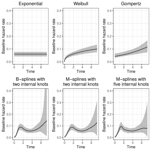
Figure 1: Estimated baseline hazards (posterior median and 95% uncertainty limits) for each of the six different models.

Figure 1 shows the resulting plot with the estimated baseline hazard for each model and 95% posterior uncertainty limits. We can clearly see from the plot the additional flexibility the cubic spline models provide. They are able to capture at least two turning points in the hazard function, one around 1.5 years and another one around 4 years. It is also interesting to note that there appears to be very little change in the fit of the M-spline model when we increase the number of internal knots from two to five.

We can also compare the fit of these models using the loo method for stansurv objects: R> compare_models(loo(mod1_exp), + loo(mod1_weibull), + loo(mod1_gompertz), + loo(mod1_bspline), + loo(mod1_mspline1), + loo(mod1_mspline2)) Model formulas: : NULL : NULL : NULL : NULL : NULL : NULL elpd_diff se_diff mod1_mspline1 0.0 0.0 mod1_bspline -0.4 1.7 mod1_mspline2 -1.6 1.5 mod1_weibull -18.0 5.3 mod1_gompertz -31.5 6.1 mod1_exp -36.3 6.0 where we see that models with a flexible parametric (spline-based) baseline hazard fit the data best followed by the standard parametric (Weibull, Gompertz, exponential) models. Roughly speaking, the B-spline and M-spline models seem to fit the data equally well since the differences in elpd between the models are very small relative to their standard errors. Moreover, increasing the number of internal knots for the M-splines from two (the default) to five doesn’t seem to improve the fit (that is the default number of knots seems to provide sufficient flexibility for modelling the baseline hazard).

After fitting the survival model we often want to estimate the predicted survival function for individuals with different covariate patterns. Therefore, let us obtain the predicted survival function between 0 and 5 years for an individual in each of the prognostic groups. To do this we can use the posterior_survfit() method for ‘stansurv’ objects and it’s associated plot() method.

First let us construct the prediction (covariate) data: R> nd <- data.frame(group = c("Good", "Medium", "Poor")) R> head(nd) group 1 Good 2 Medium 3 Poor and then generate the posterior predictions: R> ps <- posterior_survfit(mod1, + newdata = nd, + times = 0, + extrapolate = TRUE, + control = list(edist = 5)) R> head(ps) stan_surv predictions num. individuals: 3 prediction type: event free probability standardised?: no conditional?: no

id cond_time time median ci_lb ci_ub 1 1 NA 0.0000 1.0000 1.0000 1.0000 2 1 NA 0.0505 0.9999 0.9993 1.0000 3 1 NA 0.1010 0.9996 0.9987 0.9999 4 1 NA 0.1515 0.9992 0.9979 0.9997 5 1 NA 0.2020 0.9987 0.9971 0.9995 6 1 NA 0.2525 0.9981 0.9960 0.9991

Here we note that the id variable in the data frame of posterior predictions identifies which row of newdata the predictions correspond to. For demonstration purposes we have also included other arguments in the posterior_survfit() call, namely:

• the times = 0 argument says that we want to predict at time $t=0$ (i.e. baseline) for each individual in the newdata (this is the default anyway);

• the extrapolate = TRUE argument says that we want to extrapolate forward from time $t=0$ (this is also the default); and

• the control = list(edist = 5) identifies the control of the extrapolation; this is saying we wish to extrapolate the survival function forward from time $t=0$ for a distance of 5 time units (the default would have been to extrapolate as far as the largest event or censoring time in the estimation dataset, which is 7.28 years in the bcancer data).

Let us now plot the survival predictions. We will relabel the id variable with meaningful labels identifying the covariate profile of each new individual in our prediction data: