Feedback Identification of conductance-based models

Abstract

This paper applies the classical prediction error method (PEM) to the estimation of nonlinear discrete-time models of neuronal systems subject to input-additive noise. While the nonlinear system exhibits excitability, bifurcations, and limit-cycle oscillations, we prove consistency of the parameter estimation procedure under output feedback. Hence, this paper provides a rigorous framework for the application of conventional nonlinear system identification methods to discrete-time stochastic neuronal systems. The main result exploits the elementary property that conductance-based models of neurons have an exponentially contracting inverse dynamics. This property is implied by the voltage-clamp experiment, which has been the fundamental modeling experiment of neurons ever since the pioneering work of Hodgkin and Huxley.

, ,

1 Introduction

The estimation of models for biological neuronal systems is a topic that has attracted considerable interest in the scientific community over the past decades [32, 13, 19, 24, 31]. However, the asymptotic properties of published estimation methods are rarely discussed. This is understandable for models that exhibit highly nonlinear dynamics including excitable behaviors and limit cycle oscillations.

The goal of this paper is to show that rigorous convergence results can be established in the most classical framework of the prediction error method (PEM) [25, 26]. In nonlinear system identification, the convergence and consistency analysis of the PEM depends on the assumption that the signals are generated within a process with some form of input-output stability — for instance, a fading memory [4], input-output exponential stability [25, 33, 1], or mean square convergence of the output to that of a Volterra series [34, 38]. In addition, the analysis is greatly simplified by the assumption that the true system is affected by output-additive noise only [38, 27].

Neuronal models are nonlinear systems that fail to satisfy the stability and the output-additive noise assumptions. First, neuronal systems are primarily subject to input-additive noise. This type of noise models the stochastic fluctuations of currents traversing the neuronal membrane. For a review of the modeling of noise in neuronal systems, see [15, 14]. Furthermore, the non-equilibrium nature of neuronal behaviors precludes any reasonable exponential stability or fading memory assumption.

Previous works have studied the application of the PEM under these unfavorable conditions. When the noise is input-additive, the difficulty lies in the intractability of analytically computing the optimal one-step-ahead predictor (see [37] for a discussion). As long as the data-generating process is input-output exponentially stable, consistent parameter estimates can be obtained in some cases, e.g., when predictor models are linear in the past outputs [1] or when LTI elements of a block-oriented model structure are known [33]. When input-output stability is not guaranteed, as in the case of oscillatory systems, an alternative to standard PEM analysis must be found. In [7], the authors justify with dynamical systems theory the application of the PEM to identify the linear element of a Lure-type system with a limit cycle; the authors assume ergodicity of the system’s signals in order to bypass the question of stability. In [29], the authors develop a method based on transverse contraction analysis to identify oscillatory systems under the assumption that all states of the model are available; no noise considerations are made.

The main observation underlying the present paper is that while the assumptions that make PEM analysis tractable are not verified for conductance-based neuronal models, they hold for their inverse. In other words, conductance-based models verify these assumptions under high-gain output feedback. This means that neuronal systems can be identified with classical techniques by relying on the direct approach of closed-loop system identification [12]. Using contraction theory [28], we rigorously justify the use of the direct approach to consistently estimate discrete-time neuronal models.

We show that the closed-loop approach to the neuronal system identification problem is fully consistent with the classical voltage-clamp experiment of Hodgkin and Huxley [17]. Voltage-clamp has remained to date the key experimental methodology to derive a state-space model of a neuron. We show that there is flexibility in designing a contracting output feedback law beyond the high-gain implementation of voltage-clamp. As in previous work dealing with Lure systems [5], we advocate that feedback design is an integral element of neuronal system identification, which makes this an attractive application of closed-loop system identification theory.

The paper is organized as follows: in Section 2, we review a number of classical tools of nonlinear system identification and analysis. In Section 3, we introduce the general class of conductance-based models and show that they have a contracting inverse. In Section 4, we detail the identification of the inverse dynamics of discrete-time neuronal systems with the PEM and discuss the plausibility of the required assumptions. In Section 5, we illustrate our results using data from numerical simulations.

2 Preliminaries

This section reviews two classical results of system theory: the convergence properties of the prediction error method [25], and the system property of contraction [28].

We use the following notation: For a discrete-time variable $x_{k}$, the signal up to time $k$ is denoted by $x_{[0,k]}=(x_{k},x_{k-1},\dotsc,x_{0})$. We write $\mathbb{R}_{+}=[0,\infty)$, $\mathbb{N}=\{1,2,\dotsc\}$, and $\mathbb{Z}_{+}=~{}\{0,1,\dotsc\}$. The number $0$ is treated as a scalar or as a vector, with the dimension implied by the context in which it is used. The norm $\|\cdot\|$ denotes the Euclidean norm, and $\sigma_{\max}[\;\cdot\;]$ denotes the largest singular value of a matrix. For arbitrary $\beta>0$, the class of ${n_{u}}$-valued sequences $u:\mathbb{Z}_{+}\to\mathbb{R}^{n_{u}}$ such that $\sup_{k\in\mathbb{Z}_{+}}\max_{j}|u_{j,k}|<\beta$ is denoted by $\mathcal{U}_{\beta}^{n_{u}}$.

2.1 Parametric Identification of nonlinear systems with the Prediction Error Method

Consider a nonlinear stochastic discrete-time system represented by

$$y_{k}=F_{k}\left(u_{[0,k]};x_{0}\right)+e_{k}$$ (1)

where $u_{k}\in\mathbb{R}^{{n_{u}}}$ is the system’s input, $y_{k}\in\mathbb{R}^{{n_{y}}}$ is the system’s output, $e_{k}\in\mathbb{R}^{{n_{y}}}$ is a stochastic process such that $E[e_{k}\;|\;e_{[0,k-1]}]=0$, $F_{k}(\cdot)$ is a sequence of deterministic mappings, and $x_{0}$ is an initial state.

Assume that the system (1) is in a feedback loop with an adaptive feedback element given by

$$u_{k}=H_{k}\left(y_{[0,k-1]},u_{[0,k-1]},r_{k}\right)$$ (2)

where $u_{k}$ is the feedback element’s output, $y_{k}$ is the output of (1), and $r_{k}\in\mathbb{R}^{n_{r}}$ is an external signal.

In the prediction error framework, the system (1) is identified based on $N$ collected input-output data points, given by the sequences $y_{[0,N]}$ and $u_{[0,N]}$. For this purpose, a parametric model is used to obtain a prediction $\hat{y}_{k}$ of the output $y_{k}$. In this paper, we work with an output error predictor model, which is represented by a sequence of operators $\hat{F}_{k}$ such that

$$\hat{y}_{k}(\theta)=\hat{F}_{k}\left(u_{[0,k]};\theta\right)$$ (3)

where $\theta\in\mathcal{D}$ denotes a vector of parameters, and $\mathcal{D}$ is a subset of $\mathbb{R}^{n_{\theta}}$, with ${n_{\theta}}$ the number of parameters. The assumption on the process $e_{k}$ implies that (3) is the optimal mean squared error predictor of $y_{k}$, given $y_{0:k-1}$ and $u_{0:k}$.

A simple criterion that can be used to obtain estimates for the parameters in the vector $\theta$ is the minimization of the cost function

$$V_{N}(\theta)=\frac{1}{N}\sum_{k=1}^{N}\|y_{k}-\hat{y}_{k}(\theta)\|^{2},$$ (4)

resulting in the parameter estimates

$$\hat{\theta}_{N}=\text{arg}\min_{\theta\in\mathcal{D}}V_{N}(\theta)$$ (5)

The asymptotic behavior of the parameter estimates $\hat{\theta}_{N}$ as the number of data points $N$ grows to infinity depends on the asymptotic behavior of the function $V_{N}(\theta)$. Since the system is stochastic, $V_{N}(\theta)$ is a random variable. To guarantee that the identified model is independent of the specific realization of the noise entering the system, we need the prediction error $\varepsilon_{k}(\theta)=y_{k}-\hat{y}_{k}(\theta)$ to satisfy an ergodicity property: $V_{N}(\theta)$ must converge to its expected value as $N\to\infty$. This property is achieved by means of two fundamental conditions: one on the system that generates the data, and one on the predictor.

Condition 1 ([25],[12]).

The closed-loop system (1)-(2) is such that for each $k,s\in\mathbb{Z}_{+}$, $k\geq s$, there exist random variables $\bar{y}_{k,s}$ and $\bar{u}_{k,s}$, independent of $r_{[0,s]}$ and $e_{[0,s]}$ but not independent of $r_{[0,k]}$ and $e_{[0,k]}$, such that

$$E\left[\|y_{k}-\bar{y}_{k,s}\|^{4}\right] <C\alpha^{k-s}$$ (6a)

$$E\left[\|u_{k}-\bar{u}_{k,s}\|^{4}\right] <C\alpha^{k-s}$$ (6b)

for some $C>0$ and $\alpha<1$. Here, $\bar{y}_{s,s}=\bar{u}_{s,s}=0$.

Condition 2 ([25]).

The mappings $\hat{F}_{k}$ are differentiable with respect to $\theta$ for all $\theta\in\mathcal{D}$, where $\mathcal{D}$ is a closed and bounded subset of $\mathbb{R}^{n_{\theta}}$. Furthermore, there exist a $C<\infty$ and $\alpha\in(0,1)$ such that

$$\begin{split}\big{\|}\hat{F}_{k}\left(u_{[0,k]};\theta\right)-&\hat{F}_{k}\left(\tilde{u}_{[0,k]};\theta\right)\big{\|}\\ &\leq C\sum_{m=0}^{k}\alpha^{k-m}\;\|u_{m}-\tilde{u}_{m}\|\end{split}$$ (7)

and

$$\big{\|}\hat{F}_{k}\left(0_{[0,k]};\theta\right)\big{\|}\leq C$$ (8)

for all $k$, $u_{[0,k]}$, $\tilde{u}_{[0,k]}$, and $\theta$ belongs to an open neighborhood of $\mathcal{D}$. The $(d/d\theta)\hat{F}_{k}$ are subject to an inequality analogous to (7).

When the model (3) satisfies Condition 2, then the mapping $\theta\mapsto\{\hat{F}_{k}(\;\cdot\;;\theta)\}_{k\in\mathbb{Z}_{+}}$ is called a model structure [26, Section 5.7]. Thus (3) is called a model structure when viewed as a function of $\theta$.

The main result of [25] can now be stated as follows.

Lemma 1 ([25]).

Consider the feedback system (1)-(2) subject to Condition 1, and the model (3) subject to Condition 2. Consider $V_{N}(\theta)$ given by (4). Then

$$\sup_{\theta\in\mathcal{D}}\left|V_{N}(\theta)-E\left[V_{N}(\theta)\right]\right|\to 0\quad\quad\text{ w.p. }1\text{ as }N\to\infty$$

2.2 Contracting discrete-time dynamics

Neuronal systems are most commonly represented by state-space models, and so we will rely on the state-space formalism of contraction theory [28] to analyze the identification problem. We present both the discrete-time and continuous-time definitions in sequence, as they are both relevant to us.

First, consider the discrete-time system

$$x_{k+1} =f(x_{k},u_{k})$$ (9a)

$$y_{k} =h(x_{k},u_{k})$$ (9b)

where $f$ and $h$ are continuously differentiable functions, $u:\mathbb{Z}_{+}\to\mathbb{R}^{n_{u}}$ is the input signal, $y:\mathbb{Z}_{+}\to\mathbb{R}^{n_{y}}$ is the output signal, and $x:\mathbb{Z}_{+}\to\mathbb{R}^{n_{x}}$ is the state vector. We denote by $x_{k}=\phi_{k,s}(u,x_{s})$ the solution of (9a) that starts at time $s$ and is evaluated at time $k\geq s$, when (9a) is subject to the input sequence $u=u_{[0,\infty]}$ and initial condition $x_{s}$. We say a set $X~{}\subseteq~{}\mathbb{R}^{{n_{x}}}$ is positively invariant, uniformly on $U\subseteq\mathbb{R}^{{n_{u}}}$, if $\phi_{k,0}(u,x_{0})\in X$ for $x_{0}\in X$, $u_{k}\in U$, and $k\in\mathbb{Z}_{+}$.

Definition 2 ([28]).

The discrete-time dynamics (9a) is said to be exponentially contracting in a set $X~{}\subseteq~{}\mathbb{R}^{{n_{x}}}$, uniformly (in $u$) on $U\subseteq\mathbb{R}^{{n_{u}}}$, if there exist a symmetric matrix sequence $P_{k}(x)\geq\epsilon I>0$ and a constant $\alpha\in(0,1)$ such that

$$\frac{\partial f}{\partial x}^{\top}P_{k+1}(f(x,u))\frac{\partial f}{\partial x}\leq\alpha^{2}P_{k}(x)$$ (10)

for all $k\in\mathbb{Z}_{+}$, $x\in X$, and $u\in U$.

We call $P_{k}(x)$ the contraction metric, and $\alpha$ the contraction rate. The result below will be instrumental in connecting the contraction property to the PEM conditions of the previous section. For simplicity, we work with a constant contraction metric.

Lemma 3.

Consider the discrete-time system (9). Let

$$y_{k}=F_{k}(u_{[0,k]};x_{0})=h(\phi_{k,0}(u,x_{0}),u_{k})$$ (11)

For some $\beta>0$, assume (9a) is exponentially contracting in a positively invariant, convex, closed and bounded set $X$, uniformly on $U~{}=~{}[-\beta,\beta]^{{n_{u}}}$, with a constant $P>0$. Then there are $C_{1},C_{2}>0$ and $\alpha\in(0,1)$ such that

$$\begin{split}&\big{\|}F_{k}\left(u_{[0,k]};x_{0}\right)-F_{k}\left(\tilde{u}_{[0,k]};\tilde{x}_{0}\right)\big{\|}\\ &\leq C_{1}\sum_{m=0}^{k}\alpha^{k-m}\|u_{m}-\tilde{u}_{m}\|+C_{2}\,\alpha^{k}\|x_{0}-\tilde{x}_{0}\|\end{split}$$ (12)

for all $k\geq 0$, $u,\tilde{u}\in\mathcal{U}_{\beta}^{n_{u}}$, and $x_{0},\tilde{x}_{0}\in X$.

Proof 2.1.

See the Appendix A.1.

2.3 Contracting continuous-time dynamics

Consider the continuous-time nonlinear system

$$\dot{x}(t)=f(x(t),u(t))$$ (13)

where $f$ is a continuously differentiable function, $u:~{}\mathbb{R}_{+}\to\mathbb{R}^{n_{u}}$ is an input signal and $x:\mathbb{R}_{+}\to\mathbb{R}^{n_{x}}$ is the state vector.

Definition 4.

The continuous-time dynamics (13) is said to be exponentially contracting in a set $X~{}\subseteq~{}\mathbb{R}^{{n_{x}}}$, uniformly (in $u$) on $U~{}\subseteq~{}\mathbb{R}^{{n_{u}}}$, if there exists a continuously differentiable symmetric matrix $P(x,t)\geq\epsilon I>0$ and a constant $\lambda>0$ such that

$$\frac{\partial f}{\partial x}^{\top}P(x,t)+P(x,t)\frac{\partial f}{\partial x}+\dot{P}(x,u,t)\leq-2\lambda P(x,t)$$ (14)

for all $t\in\mathbb{R}_{+}$, $x\in X$, and $u\in U$.

Alternatively, by writing $P=\Theta^{\top}\Theta$, (14) can be written as $\tfrac{1}{2}\left(F+F^{\top}\right)\leq-\lambda I$, with

$$F=\left(\dot{\Theta}+\Theta\frac{\partial f}{\partial x}\right)\Theta^{-1},$$

3 Conductance-based models under feedback

Conductance-based models are biophysical neuronal models that admit the circuit representation shown in Figure 1. While the framework of the present paper holds for multiple-input-multiple-output models, we focus on the single-input single-output case. Such models were first introduced in the seminal work of Hodgkin and Huxley [17]. For a general introduction, the reader is referred to Chapters 3 and 5 in [21], or textbooks of neurophysiology such as [16, 20, 11]. To date, conductance-based modeling remains the central paradigm of biophysical neuronal modeling [2].

Our main results will concern the identification of discrete-time stochastic conductance-based models. However, it is relevant to first introduce these models in a continuous-time and deterministic setting (Section 3.1). This allows us to prove the output contraction property (Section 3.2), which is central to our results. This property is also satisfied by discrete-time conductance-based models, which we introduce, along with the noise setting, at the end of the section.

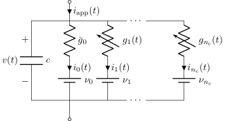
Figure 1: Schematic representation of a neuronal system.

3.1 Conductance-based models

In a conductance-based model, the neuronal membrane is modeled by an ideal capacitor of capacitance $c>0$. The voltage across the membrane, which is the output of the model, is given by $v(t)\in\mathbb{R}$. The neuron possesses ${n_{\text{c}}}\in\mathbb{N}$ different types of ion channels embedded in its membrane. These ion channels allow ionic currents to flow across the membrane according to Kirchhoff’s law,

$$c\,\dot{v}(t)=-\sum_{j=0}^{{n_{\text{c}}}}i_{j}(t)+i_{\text{app}}(t)$$ (15)

where each current $i_{j}(t)$, $j=1,\dotsc,{n_{\text{c}}}$, models an ionic current. The ionic currents not explicitly included in the model are lumped into a leak current $i_{0}(t)$. In addition, the membrane voltage is affected by an external applied current $i_{\text{app}}(t)$.

All currents in a conductance-based model obey Ohm’s law. The leak current

$$i_{0}(t)=\bar{g}_{0}(v(t)-\nu_{0})$$ (16)

is characterized by a constant conductance $\bar{g}_{0}>0$ and a constant reversal potential $\nu_{0}\in\mathbb{R}$. In contrast, the conductances of the ionic currents are voltage-dependent. This dependence is the key source of nonlinearity of conductance-based models. Owing to the original proposal of Hodgkin and Huxley, each ionic current has a nonlinear state-space model of the form

$$\tau_{m,j}(v)\,\dot{m}_{j} =-m_{j}+m_{\infty,j}(v)$$ (17a)

$$\tau_{h,j}(v)\,\dot{h}_{j} =-h_{j}+h_{\infty,j}(v)$$ (17b)

$$i_{j}(t) =\bar{g}_{j}m_{j}(t)^{\alpha_{j}}h_{j}(t)^{\beta_{j}}(v(t)-\nu_{j})$$ (17c)

with $j=1,\dotsc,{n_{\text{c}}}$. The constants $\bar{g}_{j}>0$ are called the maximal conductances, and $\nu_{j}\in\mathbb{R}$ are called reversal potentials. The variables $m_{j}$ and $h_{j}$ are called gating variables, and take values in the closed interval $[0,1]$. Their dynamics are defined by the continuously differentiable time-constant functions

$$\tau_{m,j},\tau_{h,j}:\mathbb{R}\to[\tau_{\min},\tau_{\max}]\subset\mathbb{R}_{+}$$

and activation functions

$$m_{\infty,j},h_{\infty,j}:\mathbb{R}\to[0,1]$$

where $\tau_{\min}>0$. The gating variables modulate the current conductance with a voltage-dependent first-order lag dynamics. The exponents $\alpha_{j}$ and $\beta_{j}$ belong to $\mathbb{Z}_{+}$, and whenever $\alpha_{j^{*}}=0$ or $\beta_{j^{*}}=0$, we ignore (17a) or (17b) for $j=j^{*}$, respectively. These exponents, along with the gating variable dynamics (17a)-(17b), constitute the kinetic model of the $j^{\text{th}}$ ion channel [21, 16].

A compact representation of the entire model (15)-(17) has the state-space structure

$$c\,\dot{v} =-g(v,w)+i_{\text{app}}$$ (18a)

$$\dot{w} =A(v)w+b(v)$$ (18b)

where the vector $w\in[0,1]^{n_{w}}$ collects all the gating variables $m_{j}$ and $h_{j}$ for which $\alpha_{j}>0$ and $\beta_{j}>0$, respectively, and

$$g(v,w)=\bar{g}_{0}(v-\nu_{0})+\sum_{j=1}^{{n_{\text{c}}}}\bar{g}_{j}\,m_{j}^{\alpha_{j}}\,h_{j}^{\beta_{j}}(v-\nu_{j})$$ (19)

denotes the total membrane internal current. Note that the matrix $A(v)$ is diagonal, and $b(v)$ is a vector-valued function of $v$. The model (18), with input $i_{\text{app}}$ and output $v$, is in the standard global normal form of nonlinear systems [6]. The dynamics (18b) is called the internal dynamics of the system. An important fact about (18) is that the first derivative of the output explicitly depends on the input, while the internal dynamics does not — in other words, (18) has a relative degree of one. This fact will be explored later on.

Example 5.

The Hodgkin-Huxley (HH) model [17] is the prototypical conductance-based model. It is given by (15), with $c=1$ $\mathrm{\upmu F/cm^{2}}$, and it has two ionic currents (${n_{\text{c}}}=2$): a sodium current $i_{\text{Na}}$, and a potassium current $i_{\text{K}}$. It also includes a leak current $i_{\text{L}}$. The currents are given by

$$\begin{split}i_{0}&=i_{\text{L}}=0.3\,(v+54.4)\\ i_{1}&=i_{\text{Na}}=120\,m_{\text{Na}}^{3}h_{\text{Na}}(v-55)\\ i_{2}&=i_{\text{K}}=36\,m_{\text{K}}^{4}(v+77)\\ \end{split}$$ (20)

The three internal variables are the sodium activation $m_{1}=m_{\text{Na}}$, sodium inactivation $h_{1}=h_{\text{Na}}$, and potassium activation $m_{2}=m_{\text{K}}$ (there is no potassium inactivation in the model, i.e., $\beta_{2}=0$). The vector $w$ collecting these variables is given by $w=(m_{1},h_{1},m_{2})^{\top}=(m_{\text{Na}},h_{\text{Na}},m_{\text{K}})^{\top}$. The different voltage dependent time-constants $\tau(v)$ and activation functions $m_{\infty}(v)$ and $h_{\infty}(v)$ are illustrated in Figure 2, and are detailed in Appendix B.

Each gating variable remains in the interval $[0,1]$, and, in the absence of external inputs, the voltage remains in the interval $[\nu_{2},\nu_{1}]=[\nu_{\text{K}},\nu_{\text{Na}}]=[-77,55]$. This is illustrated in Figure 3, where a spiking limit cycle oscillation occurs in response to a small constant input.

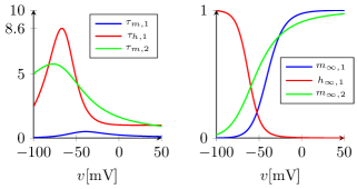
Figure 2: Left: Time constant functions in the Hodgkin-Huxley model. Right: Activation functions in the Hodgkin-Huxley model.

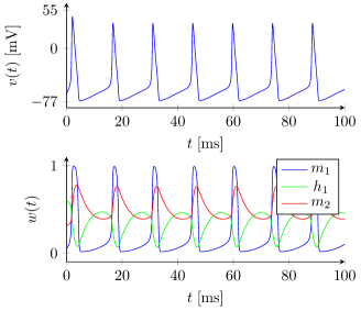
Figure 3: Simulated state trajectories of the Hodgkin-Huxley model (Example 5) for $i_{\text{app}}(t)=10\;\mathrm{\upmu A/cm^{2}}$.

The internal dynamics (18b) of the Hodgkin-Huxley model in Example 5 is exponentially contracting in $\mathbb{R}^{3}$, uniformly in $v$ on $\mathbb{R}$ (see Definition 4). This is verified with the constant metric $P=pI$, for any $p>0$, and any $\lambda$ such that $0<\lambda<1/\tau_{\max}$: in that case, we have

$$-2\,p\,\mathrm{diag}\left(\tfrac{1}{\tau_{m,1}(v)},\tfrac{1}{\tau_{h,1}(v)},\tfrac{1}{\tau_{m,2}(v)}\right)\leq-\tfrac{2}{\tau_{\max}}pI$$

and we could pick, for instance, $\lambda<1/8.6$ (see Figure 2, left). This is in fact a general property of conductance-based models:

Proposition 6.

The internal dynamics (18b) of (17)-(19) is exponentially contracting in $\mathbb{R}^{{n_{w}}}$, uniformly in $v$ on $\mathbb{R}$, i.e., there is a $P_{w}>0$ and a $\lambda_{w}>0$ such that

$$P_{w}A(v)+A(v)^{\top}P_{w}\leq-2\lambda_{w}P_{w}$$ (21)

for all $v\in\mathbb{R}$.

3.2 Output feedback contraction

A direct consequence of Proposition 6 is that a conductance-based model has a stable inverse. More precisely, using a static output feedback law, the closed-loop dynamics can be made exponentially contracting:

Proposition 7.

Consider a conductance-based model (17)-(19) subject to the output feedback law

$$i_{\text{app}}(t)=\gamma(r(t)-v(t)),$$ (22)

where $\gamma>0$ is a constant gain, and $r(t)\in\mathbb{R}$ is a reference input. Let $\{V_{\gamma}\}$ be a family of closed and bounded intervals of the real line, uniformly in $\gamma>0$. Then, there is a gain $\gamma>0$ such that the closed-loop dynamics given by (18) and (22) is exponentially contracting in $V_{\gamma}\times[0,1]^{n_{w}}$, uniformly in $r$ on $\mathbb{R}$.

Proof 3.1.

We follow an argument similar to [40, Section 2.2]. The Jacobian (with respect to the states) of the closed-loop dynamics (18), (22) is given by

$$J=\left[\begin{array}[]{cc}-\tfrac{1}{c}(\tfrac{\partial g}{\partial v}+\gamma)&-\tfrac{1}{c}\tfrac{\partial g}{\partial w}\\ \tfrac{\partial A}{\partial v}w+\tfrac{\partial b}{\partial v}&A(v)\end{array}\right]$$

(we omit dependencies on $w$ and $v$ for clarity). By Proposition 6, the internal dynamics (18b) has a contraction metric $P_{w}=\Theta_{w}^{\top}\Theta_{w}>0$ associated with the rate $\lambda_{w}>0$. We will use the matrix

$$\Theta=\left[\begin{array}[]{cc}c&0\\ 0&\Theta_{w}\end{array}\right]$$

to define a contraction metric $P=\Theta^{\top}\Theta$ for the closed-loop system. Define $F=\Theta J\Theta^{-1}$ (this is the generalized Jacobian of the closed-loop system). Then

$$F=\left[\begin{array}[]{cc}F_{11}&-\tfrac{\partial g}{\partial w}\;\Theta_{w}^{-1}\\ \tfrac{1}{c}\Theta_{w}\;\left(\tfrac{\partial A}{\partial v}w+\tfrac{\partial b}{\partial v}\right)&F_{22}\end{array}\right]$$

with

$$F_{11}=-\tfrac{1}{c}\left(\tfrac{\partial g}{\partial v}+\gamma\right)$$ (23)

and

$$F_{22}=\Theta_{w}A(v)\Theta_{w}^{-1}$$ (24)

We will use $F\prec 0$ to denote $\tfrac{1}{2}(F+F^{\top})\leq-\epsilon I$ for all $(v,w^{\top})\in V_{\gamma}\times[0,1]^{n_{w}}$ and some $\epsilon>0$. By Definition 4, to demonstrate contraction of the closed-loop system, we have to show that $F\prec 0$. To do that, we will require that $F_{11}\prec 0$ and $F_{22}\prec 0$. Contraction of the internal dynamics (Proposition 6) automatically implies

$$\tfrac{1}{2}\left(F_{22}+F_{22}^{\top}\right)\leq-\lambda_{w}I$$ (25)

for all $(v,w^{\top})\in\mathbb{R}^{{n_{w}}+1}$, and thus $F_{22}\prec 0$. Furthermore,

$$\frac{\partial g}{\partial v}(v,w)=\bar{g}_{0}+\sum_{j=1}^{{n_{\text{c}}}}\bar{g}_{j}m_{j}^{\alpha_{j}}h_{j}^{\beta_{j}}\geq\bar{g}_{0}>0$$ (26)

for $w\in[0,1]^{n_{w}}$ and thus $F_{11}\prec 0$ as well. Since $F_{11}\prec 0$, by a standard Schur complement result [18, pp. 472], we have $F\prec 0$ if and only if

$$\tfrac{1}{2}(F_{22}+F_{22}^{\top})<Q^{\top}F_{11}^{-1}Q$$ (27)

where $Q$ is the row vector given by

$$Q=\frac{1}{2}\left(-\tfrac{\partial g}{\partial w}\;\Theta_{w}^{-1}+\tfrac{1}{c}\left(\tfrac{\partial A}{\partial v}w+\tfrac{\partial b}{\partial v}\right)^{\top}\Theta_{w}^{\top}\right)$$ (28)

From (23), (26), (25) and (27), $F\prec 0$ if and only if

$$\gamma I>c\left[-\tfrac{1}{2}(F_{22}+F_{22}^{\top})\right]^{-1}Q^{\top}Q-\tfrac{\partial g}{\partial v}$$ (29)

By (25) and (26), a sufficient condition for (29) to hold is

$$\gamma>\frac{c}{\lambda_{w}}\sigma_{\max}[Q]^{2}$$ (30)

where $\sigma_{\max}[Q]$ is the largest singular value of $Q$.

Since the continuous functions $\partial g/\partial w$, $\partial A/\partial v$ and $\partial b/\partial v$ in (28) are bounded on any closed and bounded $V_{\gamma}\times~{}[0,1]^{n_{w}}$, it follows that $\sigma_{\max}[Q]$ is also bounded on such a set. Since, by assumption, $V_{\gamma}$ is uniformly bounded in $\gamma$, a sufficiently large $\gamma$ ensures that (30) is satisfied on some $V_{\gamma}\times[0,1]^{n_{w}}$.

The expressions (29) and (30) can be used to estimate a lower bound on the gain that is necessary to make a conductance-based model contracting in a given region of state-space. Depending on the choice of the contraction metric $P_{w}$, this bound can of course be conservative, as illustrated by the following example.

Example 8.

For the Hodgkin-Huxley model (Example 5), choose $P_{w}=I$ and $\lambda_{w}=1/8.6<1/\tau_{\max}$. Consider the set $[-77,55]\times[0,1]^{3}$. Computing the right-hand side of (29) for $v=-77$, $m_{1}=h_{1}=m_{2}=1$, and $\Theta_{w}=I$, leads to the lower bound of $5.1\times 10^{8}$ $\mathrm{mS/cm^{2}}$ on the gain necessary to ensure exponential contraction of the closed-loop system. Alternatively, consider the contraction metric $P_{w}=10^{6}\times\text{diag}(0.21,3.80,3.16)$. In this case, a random search over the set $[-77,55]\times[0,1]^{3}$ gives a less conservative lower bound of $2.7\times 10^{3}$ $\mathrm{mS/cm^{2}}$.

3.2.1 Non-ohmic ion currents

Instead of the Ohmic ionic current (17c), we could have used the more general formulation

$$i_{j}=\bar{g}_{j}m^{\alpha_{j}}_{j}h^{\beta_{j}}_{j}p_{j}(v)$$

with

$$p_{j}(v)=\sum_{\ell=0}^{d_{j}}\eta_{\ell}\,v^{\ell}$$

where each $d_{j}$ is an arbitrarily large polynomial degree, and $\eta_{\ell}\in\mathbb{R}$. In most non-Ohmic ionic current models, $p_{j}(v)$ is a monotonically increasing function [21, Chapter 3], and the reversal potential $\nu_{j}\in\mathbb{R}$ is the value where $p(\nu_{j})=0$. In this case, just as in the Ohmic case, we have

$$\text{sign}(p_{j}(v))=\text{sign}(v-\nu_{j}),$$ (31)

where by convention $\text{sign}\;0=0$. Since the vast majority of ionic current models is Ohmic, we keep the formulation (17c), noting that all our results can be easily adapted to encompass non-Ohmic currents such that (31) holds.

3.2.2 The voltage-clamp experiment

The output contraction property of conductance-based models is a consequence of the very experimental protocol that has been used to identify neuronal systems in the past: the voltage-clamp experiment, pioneered by Hodgkin and Huxley. The voltage-clamp experiment is nothing but a high-gain output feedback experimental protocol employed to stabilize the neuron and to determine its inverse dynamics through step response experiments. The principle of that experiment is illustrated in Figure 4. In the limit of high-gain feedback, the current drawn from the amplifier to clamp the voltage to the reference $r(t)$ is by definition the output of the internal dynamics driven by the voltage $v(t)=r(t)$. Electrophysiologists rely on the stability of that inverse system to model the internal dynamics through a series of step responses. In that sense, the contraction property of conductance-based models is an experimental property of neurons rather than the property of a specific mathematical model of the ionic currents.

Figure 4: The voltage-clamp experiment: electrodes are used to inject the current $i_{\text{app}}(t)$ and measure the voltage $v(t)$ of the neuronal membrane. The amplifiers are ideal differential amplifiers, and $\bar{g}_{e}$ models the electrode conductance. When $\bar{\gamma}\gg 1$, this implements the feedback law (22) with $\gamma=\bar{\gamma}\bar{g}_{e}$.

Models of specific ion channel types have been accumulated over time by electrophysiologists. Today, online databases such as ModelDB [30] contain large libraries of ion channels models. The structure of those models is often used in parametric identification of new types of neurons (see, e.g., [10, 19]). The identified parameters include the maximal conductances $\bar{g}_{j}$ and the Nersnt potentials $\nu_{j}$. The purpose of the next sections will be to show that the classical PEM provides consistent estimates for these parameters.

3.3 Discrete-time stochastic conductance-based models

We now turn to the task of identifying a conductance-based model from sampled current-voltage data, while taking into account the intrinsic noise that affects neuronal systems. Given a sampling period $t_{s}>0$, we will consider the discrete-time stochastic model

$$c\tfrac{v_{k+1}-v_{k}}{t_{s}} =-g(v_{k},w_{k})+\gamma(r_{k}-v_{k})+e_{k}$$ (32a)

$$\tfrac{w_{k+1}-w_{k}}{t_{s}} =A(v_{k})w_{k}+b(v_{k}),$$ (32b)

which is a forward-Euler discretization of the closed-loop system given by (17)-(19) and (22), with an additive noise $e_{k}$ on the input current. The noise current $e_{k}$ is used to model the aggregate effect of ion channel fluctuations [15, 35] and background neuronal activity [14, Chapter 8]. This system is illustrated in Figure 5.

Figure 5: Block-diagram of the system (32).

The discretization scheme leading to (32) is classical in system identification of biological neurons [19] and in simulations of neuronal behavior [23, 39, 3]. While more advanced discretization schemes could be considered, we stress that both the stochastic discrete-time model (32) and the deterministic continuous-time model (17)-(19) are empirical mean-field approximations of the molecular dynamics governing the opening and closing of ion channels [16]. For this reason, one should not regard (32) as an approximation of the continuous-time model, but merely as its discrete-time stochastic counterpart. It is also worth noting that an advanced discretization method tailored for nonlinear systems in global normal form [41] cannot improve on the forward-Euler scheme when the continuous-time system has a relative degree of one — which is the case for (18).

The remainder of the paper will address the parametric identification of (32). The next result shows that when the inputs are bounded, we can always find a positively invariant set in which discrete-time conductance-based models can be made contracting by output feedback:

Proposition 9.

Consider the system (32). Assume that $|r_{k}|,|e_{k}|<\beta$ for all $k\geq 0$; there exist a large enough $\gamma>~{}0$, a small enough $t_{s}>~{}0$, and an interval $[v_{\min},v_{\max}]\subset\mathbb{R}$ such that $[v_{\min},v_{\max}]~{}\times~{}[0,1]^{n_{w}}$ is a positively invariant set for (32), and (32) is exponentially contracting in $[v_{\min},v_{\max}]~{}\times~{}[0,1]^{n_{w}}$, uniformly in $(r,e)$ on $[-\beta,\beta]^{2}$. Furthermore, there is a small enough $t_{s}>0$ such that $[0,1]^{n_{w}}$ is a positively invariant set for the subsystem (32b), and (32b) is exponentially contracting in $[0,1]^{n_{w}}$, uniformly in $v$ on $\mathbb{R}$.

Proof 3.2.

See Appendix A.2.

4 Identification of neuronal models with the PEM

In this section, we discuss the problem of parametric identification of the discrete-time stochastic conductance-based model (32). In Section 4.1, we frame the problem as one of closed-loop system identification, and in Section 4.2, we treat the case in which we can consistently identify the system’s capacitance, maximal conductances and reversal potentials.

4.1 Data-generating system

Since the data is generated by (32), we could attempt to identify a discrete-time conductance-based model by considering the setup shown in Figure 5. However, in that setup, the input-additive noise and the system nonlinearities make it difficult to obtain an optimal one-step-ahead predictor for the output $v_{k}$. If the noise in the measurements of $v_{k}$ is negligible, we can avoid this issue by viewing (32) as a feedback interconnection, and identifying the component in the interconnection for which $e_{k}$ becomes output-additive noise, and $v_{k}$ becomes an input. This is achieved by partitioning (32) into

$$v_{k+1} =v_{k}-t_{s}y_{k}$$ (33a)

$$u_{k} =\left[\begin{array}[]{c}u_{1,k}\\ u_{2,k}\end{array}\right]=\left[\begin{array}[]{c}\gamma(r_{k}-v_{k})\\ v_{k}\end{array}\right]$$ (33f)

and

$$w_{k+1} =w_{k}+t_{s}\left(\,A(u_{2,k})w_{k}+b(u_{2,k})\,\right)$$ (34a)

$$y_{k} =\frac{1}{c}(\,\sum_{j=1}^{{n_{\text{c}}}}\bar{g}_{j}\,m_{j,k}^{\alpha_{j}}\,h_{j,k}^{\beta_{j}}(u_{2,k}-\nu_{j})$$ (34b)

$$\hskip 40.00006pt+\bar{g}_{0}(u_{2,k}-\nu_{0})-u_{1,k}-e_{k}\,)$$

where $w$ collects the states $m_{j}$ and $h_{j}$ for which $\alpha_{j},\beta_{j}~{}>~{}0$, and $A(\cdot),b(\cdot)$ are determined by (17a)-(17b).

Most of the dynamics (and any unknown parameters) of (32) are concentrated in the subsystem (34), which has an input $u_{k}$, an output $y_{k}$, and is subject to output-additive noise $-e_{k}/c$. It is on the identification of (34) that we will focus. This is a closed-loop identification problem (see Section 2.1): in particular, if $\phi^{w}_{k,0}(u_{2},w_{0})$ is the solution of (34a), the signal $y_{k}$ can be written in the form (1), with

$$F_{k}\left(u_{[0,k]};w_{0}\right)=\tfrac{1}{c}\left(\,g(u_{2,k},\phi^{w}_{k,0}(u_{2},w_{0})\,)-u_{1,k}\right)$$ (35)

where $g(\cdot,\cdot)$ is given by (19). Similarly, $u_{k}$ can be written in the form (2). This leads to the setup in Figure 6.

Assumption 10.

The noise $e_{k}$ in (34b) is a sequence of independent random variables with $E[e_{k}]=0$ and a finite variance $E[e_{k}^{2}]=\sigma_{e}^{2}>0$. All realizations of $e$ belong to $\mathcal{U}_{\beta}$.

Assumption 11.

The signals $r_{k}$ and $v_{k}$ are exactly known (no measurement noise), and $r$ is a deterministic signal that belongs to $\mathcal{U}_{\beta}$.

Assumption 11 is consistent with the voltage-clamp experiment: it allows for current noise but assumes that the voltage is perfectly measured.

Assumption 12.

The closed-loop dynamics (33)-(34) is exponentially contracting in a positively invariant set $[v_{\min},v_{\max}]\times[0,1]^{{n_{w}}}$, uniformly on $[-\beta,\beta]^{2}$. Additionally, $(v_{0},w_{0}^{\top})\in[v_{\min},v_{\max}]\times[0,1]^{{n_{w}}}$.

It follows directly from Proposition 9 that Assumption 12 can always be verified for large enough $\gamma>0$ and small enough $t_{s}>0$. Notice that since the system parameters are unknown prior to identification, in practice we cannot check contraction of the closed-loop system by direct calculations. An experimental alternative is to probe the system and check whether input-output properties implied by contraction are verified. Such properties include exponential convergence to a unique equilibrium point, under constant input (implied by Lemma 3), and entrainment by periodic inputs [36, Theorem 2]. We will return to this point in Section 5.

Lemma 13.

Under Assumptions 10-12, the closed-loop system (33)-(34) satisfies Condition 1.

Proof 4.1.

See the Appendix A.3.

Figure 6: Block-diagram of the feedback system (33)-(34). The mappings $F_{k}$ are given by (35).

4.2 Identification with fixed ion channel kinetics

Recall that the dynamics (34a), as well as the exponents $\alpha_{j}$, $\beta_{j}$ in (34b), are determined by ion channel kinetic models. Given a library of known ion channel kinetic models, we will concentrate on identifying the parameters $c$, $\bar{g}_{j}$, and $\nu_{j}$ in (34b), for $j=0,1,\dotsc,{n_{\text{c}}}$. This can be achieved by postulating a predictor model containing ${n_{\text{m}}}\geq{n_{\text{c}}}$ known ion channel kinetic models, chosen a priori.

For $j=1,\dotsc,{n_{\text{m}}}$, let the predictor states be given by $\hat{m}_{j}$ and $\hat{h}_{j}$; to each of these states, we associate the exponents $\hat{\alpha}_{j}\in\mathbb{Z}_{+}$ and $\hat{\beta_{j}}\in\mathbb{Z}_{+}$, respectively. We define the predictor by

$$\hat{w}_{k+1} =\hat{w}_{k}+t_{s}(\hat{A}(u_{2,k})\hat{w}_{k}+\hat{b}(u_{2,k}))$$ (36a)

$$\hat{y}_{k}(\theta) =\sum_{j=1}^{{n_{\text{m}}}}\hat{m}_{j,k}^{\hat{\alpha}_{j}}\,\hat{h}_{j,k}^{\hat{\beta}_{j}}\,(\theta_{j}^{(1)}+\theta_{j}^{(2)}u_{2,k})$$ (36b)

$$\hskip 40.00006pt+\theta_{0}^{(1)}+\theta_{0}^{(2)}u_{2,k}+\theta^{(3)}u_{1,k}$$

where $u_{1,k}$ and $u_{2,k}$ are given by (33f), the vector $\hat{w}$ collects the gating variables $\hat{m}_{j}$ and $\hat{h}_{j}$ for which $\hat{\alpha}_{j}>0$ and $\hat{\beta_{j}}>0$, respectively, and $\theta^{(1)},\theta^{(2)}\in\mathbb{R}^{{n_{\text{m}}}\times 1}$ and $\theta^{(3)}\in\mathbb{R}$ are predictor parameters. The predictor states evolve analogously to the (forward-Euler) discretized version of (17a)-(17b), but with activation and time constant functions given by $\hat{\tau}_{m,j}(\cdot)$, $\hat{\tau}_{h,j}(\cdot)$, $\hat{m}_{\infty,j}(\cdot)$ and $\hat{h}_{\infty,j}(\cdot)$.

Comparing (34b) with (36b), we see that the predictor parameters $\theta_{j}^{(1)}$, $\theta_{j}^{(2)}$ and $\theta^{(3)}$ are meant to identify expressions involving the true system parameters $c$, $\bar{g}_{j}$ and $\nu_{j}$. To formalize this, we make the following assumption:

Assumption 14.

The model structure (36) contains the true system (34): we have $\hat{\tau}_{m,j}=\tau_{m,j}$, $\hat{\tau}_{h,j}=\tau_{h,j}$, $\hat{m}_{\infty,j}=m_{\infty,j}$, $\hat{h}_{\infty,j}=h_{\infty,j}$, $\hat{\alpha}_{j}=\alpha_{j}$ and $\hat{\beta}_{j}=\beta_{j}$ for $j=1,\dotsc,{n_{\text{c}}}\leq{n_{\text{m}}}$. Additionally, the dynamics (36a) is exponentially contracting in the positively invariant set $[0,1]^{n_{\hat{w}}}$, uniformly in $v$ on $\mathbb{R}$.

Again, it follows from Proposition 9 that Assumption 14 can always be verified for small enough $t_{s}>0$. Under Assumption 14, we now see that the true parameter vector, denoted by $\bar{\theta}=(\bar{\theta}^{(1)\top},\bar{\theta}^{(2)\top},\bar{\theta}^{(3)})^{\top}$, is given by

$$\begin{split}\bar{\theta}_{j}^{(1)}&=\left\{\begin{array}[]{ll}-\bar{g}_{j}\nu_{j}/c,&\quad j=0,1,\dotsc,{n_{\text{c}}}\\ 0,&\quad j>{n_{\text{c}}}\end{array}\right.\\ \bar{\theta}_{j}^{(2)}&=\left\{\begin{array}[]{ll}\bar{g}_{j}/c,&\quad j=0,1,\dotsc,{n_{\text{c}}}\\ 0,&\quad j>{n_{\text{c}}}\end{array}\right.\\ \bar{\theta}^{(3)}&=-1/c\end{split}$$ (37)

To simplify our results, we will assume the following:

Assumption 15.

The initial states of the true dynamics (34a) and of the predictor dynamics (36a) satisfy $\hat{m}_{j,0}=m_{j,0}$, $\hat{h}_{j,0}=h_{j,0}$ for $1\leq j\leq{n_{\text{c}}}$, and $\hat{m}_{j,0},\hat{h}_{j,0}\in[0,1]$ for ${n_{\text{c}}}<j\leq{n_{\text{m}}}$.

As long as Assumptions 12 and 14 are verified, due to the contraction property, Assumption 15 can be ensured in practice by discarding initial segments of the data.

Under Assumptions 10, 11, 14 and 15, (36) is the optimal mean squared error one-step-ahead predictor of $y_{k}$ in (34). The closed-loop identification approach thus avoids the intractability in the computation of an optimal predictor for the forward dynamics output $v_{k}$.

Collecting the parameters in a single vector $\theta\in\mathbb{R}^{2{n_{\text{c}}}+1}$ given by

$$\theta=(\theta^{(1)\top},\theta^{(2)\top},\theta^{(3)})^{\top},$$

we can more compactly write (36b) as

$$\hat{y}_{k}(\theta)=\psi_{k}\theta$$

with the row vector $\psi_{k}\in\mathbb{R}^{1\times(2{n_{\text{m}}}+1)}$ given by

$$\psi_{k}= \left(1,\;\hat{m}_{1,k}^{\hat{\alpha}_{1}}\,\hat{h}_{1,k}^{\hat{\beta}_{1}}\;,\;\dotsc\;,\;\hat{m}_{{n_{\text{m}}},k}^{\hat{\alpha}_{{n_{\text{m}}}}}\,\hat{h}_{{n_{\text{m}}},k}^{\hat{\beta}_{{n_{\text{m}}}}}\;,\;u_{2,k}\;,\right.$$

$$\left.u_{2,k}\,\hat{m}_{1,k}^{\hat{\alpha}_{1}}\,\hat{h}_{1,k}^{\hat{\beta}_{1}},\;\dotsc\;,\;u_{2,k}\;\hat{m}_{{n_{\text{m}}},k}^{\hat{\alpha}_{{n_{\text{m}}}}}\,\hat{h}_{{n_{\text{m}}},k}^{\hat{\beta}_{{n_{\text{m}}}}},\;u_{1,k}\right)$$

Gathering $\psi_{k}$ in a matrix $\Psi_{N}\in\mathbb{R}^{N\times(2{n_{\text{m}}}+1)}$ given by

$$\Psi_{N}=\left[\psi_{N}^{\top},\psi_{N-1}^{\top},\dotsc,\psi_{1}^{\top}\right]^{\top}$$ (38)

we find that the vector of model structure outputs from time $k=N$ down to time $k=1$ is given by

$$\hat{y}_{[1,N]}^{\top}(\theta)=\Psi_{N}\theta$$

The above formulation shows that the ion channel kinetic models act as basis operators mapping the input sequence $u_{[0,N]}$, given by (33f), to the columns of $\Psi_{N}$.

Assumption 16 (Persistency of excitation).

There is a $N^{*}>0$ such that $\tfrac{1}{N}\Psi_{N}^{\top}\Psi_{N}$ and $E\left[\tfrac{1}{N}\Psi_{N}^{\top}\Psi_{N}\right]$ are positive-definite for all $N>N^{*}$.

Assumption 16 is an assumption both on the model structure and on $r_{k}$, the signal used to excite the true system. Intuitively, we should not include two identical ion channel kinetics in the model structure, and the excitation signal $r_{k}$ should be sufficiently rich.

Under Assumption 11, we are able to compute

$$y_{k}=-\frac{v_{k+1}-v_{k}}{t_{s}}$$

from the measurements, and thus we can form the cost function $V_{N}(\theta)$ given by (4). There is practical relevance in the fact that a single forward difference of the voltage yields $y_{k}$, which is a consequence of the relative degree one property of neuronal models. We can now state the main identification result:

Theorem 17.

Let Assumptions 10-15 be satisfied. Let $N>N^{*}$, and let $\hat{\theta}_{N}=(\hat{\theta}_{N}^{(1)\top},\hat{\theta}_{N}^{(2)\top},\hat{\theta}_{N}^{(3)})^{\top}$ be given by

$$\begin{split}\hat{\theta}_{N}&=\arg\min_{\theta\in\mathcal{D}}V_{N}(\theta)\\ &=\arg\min_{\theta\in\mathcal{D}}\frac{1}{N}\|y_{[1,N]}^{\top}-\Psi_{N}\theta\|^{2}\end{split}$$ (39)

where $y_{k}$ and $\Psi_{N}$ are given by (34b) and (38), respectively, and $\mathcal{D}$ is a compact parameter domain containing $\bar{\theta}$, the true parameter vector (37). Then, we have $\hat{\theta}_{N}\to\bar{\theta}$ w.p. 1 as $N\to\infty$.

Proof 4.2.

By Assumptions 14 and 15, the true output $y_{k}$, given by (34b), can be written as

$$y^{\top}_{[1,N]}=\Psi_{N}\bar{\theta}-\tfrac{1}{c}e^{\top}_{[1,N]}$$

and thus we can write

$$E\left[V_{N}(\theta)\right]=\tfrac{1}{N}E\left[\|\Psi_{N}(\bar{\theta}-\theta)-\tfrac{1}{c}e^{\top}_{[1,N]}\|^{2}\right]$$

By Assumption 10, the time-delay present in the system ensures that $v_{k}$ and $w_{k}$ do not depend on $e_{k}$. We then have that

$$E\left[\Psi_{N}^{\top}e^{\top}_{[1,N]}\right]=0$$

and thus

$$E\left[V_{N}(\theta)\right]=\tfrac{1}{N}(\bar{\theta}-\theta)^{\top}E\left[\Psi_{N}^{\top}\Psi_{N}\right](\bar{\theta}-\theta)+\tfrac{1}{c}\sigma_{e}^{2}$$

Using Assumption 16, we have

$$\arg\min_{\theta\in\mathcal{D}}E\left[V_{N}(\theta)\right]=\bar{\theta}$$ (40)

for all $N>N^{*}$.

It remains to show that $\hat{\theta}_{N}$ converges to (40) w.p. 1 as $N\to\infty$. This is done by verifying Conditions 1 and 2 of Lemma 1. Condition 1 is satisfied due to Lemma 13. By Assumptions 11 and 12, $(v_{k},r_{k})$ remains in the bounded set $[v_{\min},v_{\max}]\times[-\beta,\beta]$, and thus the predictor input (33f) belongs to $\mathcal{U}_{\beta^{*}}^{2}$ for some $\beta^{*}>0$. By Assumptions 12 and 15, $\hat{w}_{0}\in[0,1]^{n_{\hat{w}}}$. It follows by Assumption 14 and Lemma 3 that the predictor (36) verifies Condition 2. Finally, Lemma 1 ensures that $V_{N}(\theta)$ converges uniformly to $E\left[V_{N}(\theta)\right]$ on the compact set $\mathcal{D}$. In view of (39) and (40), this ensures the result of the theorem.

An immediate consequence of Theorem 17 is that we are able to obtain consistent estimates $\hat{c}$, $\hat{\bar{g}}_{j}$ and $\hat{\nu}_{j}$ of the original unknown parameters of the system (34b), for $j=0,1,\dotsc,{n_{\text{c}}}$. They can be recovered from $\hat{c}_{N}=-1/\hat{\theta}^{(3)}_{N}$, $\hat{\nu}_{j,N}=-\hat{\theta}^{(1)}_{j,N}/\hat{\theta}^{(2)}_{j,N}$ and $\hat{\bar{g}}_{j,N}=-\hat{\theta}^{(2)}_{j,N}/\hat{\theta}^{(3)}_{j,N}$.

5 Examples

In this section, we illustrate the results of Section 4.2 by identifying various discrete-time neuronal models. All discrete-time models are obtained by forward-Euler discretization of their continuous-time counterparts with $t_{s}=0.005$ ms.

Example 18.

In this example, we identify the discrete-time Hodgkin-Huxley (HH) model

$$\begin{split}\tfrac{v_{k+1}-v_{k}}{t_{s}}&=-0.3(v_{k}+54.4)-\sum_{j=1}^{2}i_{j,k}+\gamma(r_{k}-v_{k})+e_{k}\\ i_{1,k}&=120\,m_{1,k}^{3}h_{1,k}(v_{k}-55)\\ i_{2,k}&=36\,m_{2,k}^{4}(v_{k}+77)\end{split}$$

where the states $m_{j}$ and $h_{j}$ are given by the forward-Euler discretization of (17a) and (17b), respectively, with activation and time-constant functions as in Example 5. We include in the model structure the two ion channel kinetics present in the true model, and identify the values of $c$, $\bar{g}_{j}$, and $\nu_{j}$ using the parameter vector $\theta$. Comparing the above expression to (36b), we have the true parameters shown in Table 1.

$\bar{\theta}_{0}^{(1)}$	$\bar{\theta}_{0}^{(2)}$	$\bar{\theta}_{1}^{(1)}$	$\bar{\theta}_{1}^{(2)}$	$\bar{\theta}_{2}^{(1)}$	$\bar{\theta}_{2}^{(2)}$	$\bar{\theta}^{(3)}$
$0.3\cdot 54.4$	$0.3$	$120\cdot-55$	$120$	$36\cdot 77$	$36$	$-1$

Table 1: True parameters of the Hodgkin-Huxley model.

As mentioned in Section 4.1, contraction of the closed-loop dynamics can be verified empirically. Figure 7 (top) illustrates the contraction observed for a gain of $\gamma~{}=~{}50$ in a series of step response experiments where the reference $r_{k}$ is first set to different baseline values, and then stepped to the same final value. In the case shown in Figure 7 (top), the voltage $v_{k}$ converges to the same steady-state no matter what the initial value was at $t=10\;\mathrm{ms}$.

To identify the HH model, we simulated a $5$-second long data-gathering experiment with the gain $\gamma=~{}50$. The reference is $r_{k}=-45+\tilde{r}_{k}$, where $\tilde{r}_{k}$ is white Gaussian noise of standard deviation $\sigma_{r}=100\,\mathrm{mV}$ that is first filtered by the zero-order hold discretization of the system $10^{2}/(s+10)^{2}$, then truncated so that $|\tilde{r}_{k}|\leq 100$ for $k\geq 0$. The input noise $e_{k}$ is white Gaussian noise of $\sigma_{e}=2.5\,\mathrm{\upmu A/cm^{2}}$ that is truncated so that $|e_{k}|\leq 20$ for $k\geq 0$. This setup resulted in a signal-to-noise ratio (between $y_{k}$ and $e_{k}$) of around $30.8$ dB. A $100\;\mathrm{ms}$ sample of the output $v_{k}$ used for identification is shown in Figure 7 (bottom). Notice that the step experiments (top) explore a voltage interval similar to that explored in the data-gathering experiment (bottom).

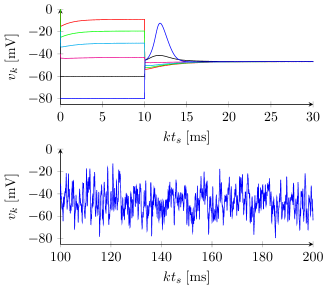
Figure 7: Voltage output $v_{k}$ of the discrete-time Hodgkin-Huxley model identified in Example 18 subject to different reference inputs $r_{k}$. Top: six experiments in which $r_{k}$ is first set to different baseline values ($-80,-60,-40,-20,0$ and $20\;\mathrm{mV}$) and then stepped (at $10\;\mathrm{ms}$) to the same final value ($-45\;\mathrm{mV}$). Bottom: a $100\;\mathrm{ms}$ sample of the voltage output used for identification.

To eliminate transient effects and satisfy Assumption 15 as close as possible, we eliminated the initial $0.5$ seconds of measurement (corresponding to $10^{5}$ samples) from all datasets. Figure 8 shows the resulting estimation error $\bar{\theta}-\hat{\theta}_{N}$ for $N=10^{5}$ to $N=9\times 10^{5}$ ($0.5$ to $4.5$ seconds) for 20 different realizations of the experiment, as well as their average; we can see from the figure that the estimates steadily converge to the true parameters.

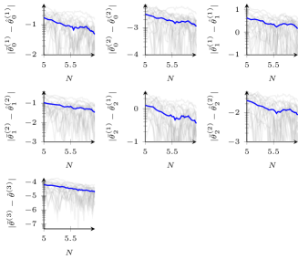
Figure 8: The $\log_{10}\times\log_{10}$ plots above show how the errors in the estimated parameters of Example 18 fall as the number of data points $N$ increases. In grey: errors in each of the 20 realizations of the identification experiment as computed for $N=10^{5}$ to $9\times 10^{5}$ ($t_{s}=0.005$). In blue: average of the 20 error traces.

Example 19.

In this example, we illustrate how a library of pre-established set of ion channel kinetic models can be used to identify different neuronal models. We consider three models, all of which are based on the system given by

$$\begin{split}\tfrac{v_{k+1}-v_{k}}{t_{s}}&=-0.3(v_{k}+17)-\sum_{j=1}^{4}i_{j,k}+\gamma(r_{k}-v_{k})+e_{k}\\ i_{1,k}&=120\,m_{1,k}^{3}\,h_{1,k}(v_{k}-55)\\ i_{2,k}&=20\,m_{2,k}^{4}(v_{k}+75)\\ i_{3,k}&=\bar{g}_{3}\,m_{3,k}^{3}\,h_{3,k}(v_{k}+75)\\ i_{4,k}&=\bar{g}_{4}\,m_{4,k}^{2}(v_{k}-120)\\ \end{split}$$

where the states $m_{j}$ and $h_{j}$ are given by the forward-Euler discretization of (17a) and (17b), respectively. The functions $m_{\infty,j}$, $h_{\infty,j}$, $\tau_{m,j}$ and $\tau_{h,j}$ are plotted in Figure 9, and are described in Appendix C.

The above system, taken from [9], defines a modified version of the Connor-Stevens neuronal model [8]. The values of the variables $\bar{g}_{3}$ and $\bar{g}_{4}$ are the distinguishing factors between the three models we use in this example. We call them Connor-Stevens (CS) models A, B, and C, according to the maximal conductance values found in Table 2.

CS model	A	B	C
$\bar{g}_{3}$	0	90	0
$\bar{g}_{4}$	0	0	0.4

Table 2: True maximal conductances in CS models A, B, and C.

Connor Stevens model A is similar to the HH model of the previous example, while models B and C differ from A due to the addition of ion currents $i_{3}$ and $i_{4}$, respectively (these currents represent an “A-type” potassium current and a calcium current, respectively). It can be verified through simulations that the addition of $i_{3}$ or $i_{4}$ makes the qualitative input-output behavior (from $i_{\text{app}}$ to $v$) of models B and C differ from that of model A. In particular, models B and C can fire periodic spikes with arbitrarily low frequency, while model A does not have that property (see, for instance, Figure 2 of [9]). The property of spiking with arbitrarily low frequency has important neurocomputational consequences. It underlies the classical distinction between Type I and Type II neuronal excitability first proposed by Hodgkin and Huxley (see [20, Chapter 7]).

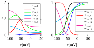
Figure 9: Left: time constant functions $\tau_{m,j}$ and $\tau_{h,j}$ in the Connor-Stevens model. Right: nonlinear activation functions $m_{\infty,j}$ and $h_{\infty,j}$ in the Connor-Stevens model.

To identify the models A, B and C, we include in a single model structure all four of the ion channels shared by those models. We simulated identification experiments in which $\gamma=50$ and $r_{k}=-45+\tilde{r}_{k}$, where $\tilde{r}_{k}$ is white Gaussian noise of standard deviation $\sigma_{r}=30\,\mathrm{mV}$ that is first filtered by the zero-order hold discretization of the system $10^{2}/(s+10)^{2}$, then truncated so that $|\tilde{r}_{k}|\leq 30$ for $k\geq 0$. The input noise $e_{k}$ is white Gaussian noise of $\sigma_{e}=1\,\mathrm{\upmu A/cm^{2}}$ that is truncated so that $|e_{k}|\leq 20$ for $k\geq 0$. This setup resulted in a signal-to-noise ratio (between $y_{k}$ and $e_{k}$) of around $28$ dB, $26$ dB and $29$ dB for the CS models A, B and C, respectively (again,we eliminated the first $0.5$ seconds of measurement from all datasets).

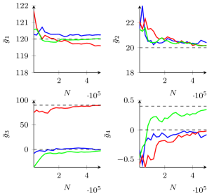
Figure 10: Evolution of the estimates of $\bar{g}_{j}$, with respect to the number of samples, for each of the identified Connor-Stevens models A (blue), B (red) and C (green). The sampling period is $t_{s}=0.005$, and the experimental setup is described in Example 19.

Figure 10 shows the evolution of the estimates of $\bar{g}_{j}$ obtained by identifying each of the CS models A, B and C (for brevity, we do not show the evolution of all parameter estimates). It can be seen that the estimates of $\bar{g}_{3}$ (or $\bar{g}_{4}$) for models that do not contain $i_{3}$ (or $i_{4}$) tend towards zero, while the other estimates tend towards their true values.

6 Conclusion

In this paper, we studied the identification of discrete-time neuronal systems under the assumption of current-additive zero-mean white noise and negligible voltage measurement noise. We showed that by treating a neuronal model as a closed-loop system, we can solve the identification problem by identifying the inverse dynamics with an output-error model structure. We have demonstrated that consistent parameter estimates are obtained when the model structure contains the internal dynamics of the system being identified. This is a common strategy adopted in neuroscience, where kinetic models of ion channels are estimated in separate experiments (see, e.g., [30]). It is worth noting that the results in this paper may hold for ion channel models which are more general than (17a)-(17b); the key requirement is that the ion channels possess a contracting dynamics, so that (21) is satisfied. Thus, this work rigorously justifies neuronal system identification using conventional methods of nonlinear identification.

Thiago Burghi was supported by the Coordenação de Aperfeiçoamento de Pessoal de Nível Superior (CAPES) – Brasil (Finance Code 001). Maarten Schoukens was supported by the European Union’s Horizon 2020 research and innovation programme under the Marie Sklodowska-Curie Fellowship (grant agreement nr. 798627). The research leading to these results has received funding from the European Research Council under the Advanced ERC Grant Agreement Switchlet n.670645. The authors thank the anonymous reviewers, as well as Dr. Monika Josza, for helping to improve earlier versions of this manuscript.

Appendix A Proofs

A.1 Proof of Lemma 3

Let $P=\Theta^{\top}\Theta$, where $\Theta>0$. Applying the change of coordinates $z_{k}=\Theta x_{k}$, we obtain the discrete-time dynamics

$$z_{k+1}=f_{\Theta}(z_{k},u_{k}),$$ (41)

where $f_{\Theta}$ is given by

$$f_{\Theta}(\zeta,\upsilon)=\Theta f\left(\Theta^{-1}\zeta,\upsilon\right).$$ (42)

By the assumptions on $X$, the set

$$Z=\{\zeta\in\mathbb{R}^{n_{x}}\;|\;\zeta=\Theta\xi,\;\xi\in X\}.$$

is closed, bounded and convex. Furthermore, $Z$ is a positively invariant set for (41), uniformly in $[-\beta,\beta]^{n_{u}}$.

Since $P=\Theta^{\top}\Theta$ with $\Theta$ invertible, the inequality (10) implies

$$\sigma_{\max}\left[\Theta\frac{\partial f}{\partial x}(x,u)\Theta^{-1}\right]\leq\alpha<1$$

for all $k\in\mathbb{Z}_{+}$, $x\in X$, and $u\in U$. From (42), this implies that $\sigma_{\max}\left[\partial f_{\Theta}/\partial\zeta\right]\leq\alpha$ on $Z\times[-\beta,\beta]^{n_{u}}$. Furthermore, since $\partial f_{\Theta}/\partial\upsilon$ is a continuous function and $Z~{}\times~{}[-\beta,\beta]^{n_{u}}$ is closed and bounded, there is some $L_{1}>0$ such that $\sigma_{\max}\left[\partial f_{\Theta}/\partial\upsilon\right]\leq L_{1}$ on $Z\times[-\beta,\beta]^{n_{u}}$.

Now, let $\zeta,\tilde{\zeta}\in Z$ and $\upsilon,\tilde{\upsilon}\in[-\beta,\beta]^{n_{u}}$. Let also $\gamma_{1}(s)~{}=~{}(1-s)\tilde{\zeta}+s\zeta$ and $\gamma_{2}(s)=(1-s)\tilde{\upsilon}+s\upsilon$, with $s\in[0,1]$. It can be shown, using the mean value theorem (see, e.g., the proof of [22, Lemma 3.1]), that there is an $s^{*}\in(0,1)$ such that

By the triangle inequality and convexity of $Z\times[-\beta,\beta]^{n_{u}}$, the above implies

$$\|f_{\Theta}(\zeta,\upsilon)-f_{\Theta}(\tilde{\zeta},\tilde{\upsilon})\|\leq\alpha\|\zeta-\tilde{\zeta}\|+L_{1}\|\upsilon-\tilde{\upsilon}\|$$ (43)

on $Z\times[-\beta,\beta]^{n_{u}}$. By positive invariance of $Z$, we are allowed to apply (41) and (43) recursively, obtaining

for $k\geq 0$. Multiplying both sides of the inequality by $\sigma_{\max}\left[\Theta^{-1}\right]$ and substituting $z_{k}=\Theta x_{k}$, we have

$$\begin{split}\|x_{k}-\tilde{x}_{k}\|\leq&\frac{L_{1}}{\sigma_{\min}}\sum_{m=1}^{k}\alpha^{m-1}\|u_{k-m}-\tilde{u}_{k-m}\|\\ &+\frac{\sigma_{\max}}{\sigma_{\min}}\;\alpha^{k}\;\|x_{0}-\tilde{x}_{0}\|\end{split}$$ (44)

for $k\geq 0$, where $\sigma_{\max}$ and $\sigma_{\min}$ denote the largest and the smallest singular values of $\Theta$, respectively.

By arguments similar to those used above, there are $L_{2},L_{3}>0$ such that

$$\|y_{k}-\tilde{y}_{k}\|\leq L_{2}\|x_{k}-\tilde{x}_{k}\|+L_{3}\|u_{k}-\tilde{u}_{k}\|$$ (45)

The result (12) follows directly from (44) and (45) by setting $C_{1}=\max\{L_{1}L_{2}\sigma_{\min}^{-1},L_{3}\}$ and $C_{2}=L_{2}\sigma_{\max}\sigma_{\min}^{-1}$.

A.2 Proof of Proposition 9

To prove Proposition 9, we first state a result concerning the contraction of forward-Euler discretized systems:

Lemma 20.

Consider the continuous-time dynamics

$$\dot{x}(t)=f(x(t),u(t))+B_{r}\,r(t),$$ (46)

where $x(t)\in\mathbb{R}^{{n_{x}}}$, $u(t)\in\mathbb{R}^{{n_{u}}}$, $r(t)\in\mathbb{R}^{{n_{r}}}$, $B_{r}$ is a constant matrix, and $f$ is continuously differentiable. Assume (46) is exponentially contracting in a set $X$, uniformly in $(u,r)$ on $\mathbb{R}^{{n_{u}}+{n_{r}}}$, with constant $P>0$ and $\lambda>0$. Assume $\partial f/\partial x$ is bounded on $X\times\mathbb{R}^{{n_{u}}}$. Let

$$\begin{split}x_{k+1}&=f_{d}(x_{k},u_{k},d_{k})\\ &:=x_{k}+t_{s}(f(x_{k},u_{k})+B_{d}\,d_{k})\end{split}$$ (47)

where $t_{s}>0$ is a sampling period, $d_{k}\in\mathbb{R}^{n_{d}}$, and $B_{d}$ is a constant matrix. Then, there exists a sufficiently small $t_{s}$ such that (47) is exponentially contracting in $X$, uniformly in $(u,d)$ on $\mathbb{R}^{{n_{u}}+n_{d}}$.

Proof A.1.

Since $\partial f/\partial x$ is bounded on $X\times\mathbb{R}^{{n_{u}}}$, there is a number $\bar{\sigma}$ such that $\bar{\sigma}\geq\sigma_{\max}[\partial f/\partial x]$ on that set. Using contraction of the continuous-time system, we have

$$\begin{split}\frac{\partial f_{d}^{\top}}{\partial x}P\frac{\partial f_{d}}{\partial x}&=\left(I+t_{s}\frac{\partial f^{\top}}{\partial x}\right)P\left(I+t_{s}\frac{\partial f}{\partial x}\right)\\ &\leq(1-2t_{s}\lambda)P+t_{s}^{2}\frac{\partial f^{\top}}{\partial x}P\frac{\partial f}{\partial x}\\ &\leq\left(1-2t_{s}\lambda+t_{s}^{2}\frac{\lambda_{\max}[P]}{\lambda_{\min}[P]}\bar{\sigma}^{2}\right)P\\ &=\alpha(t_{s})^{2}P\end{split}$$ (48)

for all $x\in X$ and $u\in\mathbb{R}^{{n_{u}}}$. The second inequality above follows from the fact that $A^{\top}PA\leq\lambda_{\max}[P]\sigma^{2}_{\max}[A]I$ and $I\leq 1/\lambda_{\min}[P]P$. Making $t_{s}<1$ small enough ensures that $\alpha(t_{s})^{2}<1$, concluding the proof.

We now carry on with the proof Proposition 9. The discretization of (17a) is given by

$$\begin{split}m_{j,k+1}&=m_{j,k}+\tfrac{t_{s}}{\tau_{m,j}(v_{k})}(-m_{j,k}+m_{\infty,j}(v_{k}))\\ &=m_{j,k}\left(1-\tfrac{t_{s}}{\tau_{m,j}(v_{k})}\right)+\tfrac{t_{s}}{\tau_{m,j}(v_{k})}m_{\infty,j}(v_{k})\end{split}$$

where $m_{\infty,j}(v_{k})\in[0,1]$ and $\tau_{m,j}(v_{k})\in[\tau_{\min},\tau_{\max}]$, with $\tau_{\min}~{}>~{}0$. It directly follows that for any $t_{s}\leq\tau_{\min}$, for all $m_{j,k}\in[0,1]$, and for all $v_{k}\in\mathbb{R}$, we have $m_{j,k+1}\in~{}[0,1]$. An analogous fact holds for $h_{j,k}$. Thus for any $t_{s}\leq\tau_{\min}$, $w_{0}\in~{}[0,1]^{n_{w}}$ implies $w_{k}\in[0,1]^{n_{w}}$ for all $k\geq 0$, and $[0,1]^{{n_{w}}}$ is positively invariant for the subsystem (32b), uniformly in $v$ on $\mathbb{R}$. Since $A(v)=-\mathrm{diag}(1/\tau_{m,1}(v),\dotsc)$ is bounded on $\mathbb{R}$, Proposition 6 together with Lemma 20 imply the existence of a $t_{s}\leq\tau_{\min}$ such that (32b) is exponentially contracting in $[0,1]^{{n_{w}}}$, uniformly on $\mathbb{R}$.

Now, let $V_{\gamma}\subset\mathbb{R}$ be the interval

$$V_{\gamma}=\left[\min_{j}\{\nu_{j},-\beta\tfrac{\gamma+1}{\gamma}\},\max_{j}\{\nu_{j},\beta\tfrac{\gamma+1}{\gamma}\}\right]$$

Let $t_{s}^{*}(\gamma)=\min\{\tau_{\min},1/\gamma\}$, and let

$$v_{\max}(\gamma)=\max_{\begin{subarray}{c}v_{k},w_{k},\\ r_{k},e_{k}\end{subarray}}v_{k}-\frac{t_{s}^{*}(\gamma)}{c}(g(v_{k},w_{k})-\gamma(r_{k}-v_{k})-e_{k})$$

where the maximum is over the closed and bounded set $V_{\gamma}\times[0,1]^{{n_{w}}}\times[-\beta,\beta]^{2}$. Defining $v_{\min}(\gamma)$ analogously, we claim that for all $\gamma>0$, $[v_{\min}(\gamma),v_{\max}(\gamma)]\times[0,1]^{n_{w}}$ is a positively invariant set for (32), uniformly on $[-\beta,\beta]^{2}$. To prove this claim, we first observe that $v_{k+1}\in[v_{\min}(\gamma),v_{\max}(\gamma)]$ whenever $(v_{k},w_{k}^{\top})\in V_{\gamma}\times[0,1]^{{n_{w}}}$ and $(r_{k},e_{k})\in[-\beta,\beta]^{2}$. If $[v_{\min}(\gamma),v_{\max}(\gamma)]\subseteq V_{\gamma}$, then the claim follows immediately from the previous observation. If, alternatively, $V_{\gamma}\subset[v_{\min}(\gamma),v_{\max}(\gamma)]$, then the claim follows from the fact that

$$\begin{array}[]{ll}v_{k+1}\geq v_{k}&\text{for all}\quad v_{k}\leq\min_{j}\{\nu_{j},-\beta(\gamma+1)/\gamma\}\\ v_{k+1}\leq v_{k}&\text{for all}\quad v_{k}\geq\max_{j}\{\nu_{j},\beta(\gamma+1)/\gamma\}\\ \end{array}$$

whenever $w_{k}\in[0,1]^{n_{w}}$ and $(r_{k},e_{k})\in[-\beta,\beta]^{2}$.

Since $[v_{\min}(\gamma),v_{\max}(\gamma)]$ is uniformly bounded in $\gamma>0$, Proposition 7 together with Lemma 20 imply the existence of a $\gamma>0$ and a $t_{s}\leq t_{s}^{*}(\gamma)$ such that (32) is exponentially contracting in $[v_{\min}(\gamma),v_{\max}(\gamma)]\times[0,1]^{n_{w}}$, uniformly in $[-\beta,\beta]^{n_{w}}$. This concludes the proof.

A.3 Proof of Lemma 13

Consider two different solutions of (33)-(34) (which, combined, can be written as (32)). The first is given by

$$\begin{split}(v_{k},w_{k}^{\top})^{\top}&=\phi_{k,0}((r,e)^{\top},(v_{0},w_{0}^{\top})^{\top})\\ \end{split}$$ (49)

for $k\geq 0$, and the second is given by

$$\begin{split}(\bar{v}_{k,s+1},\bar{w}_{k,s+1}^{\top})^{\top}&=\phi_{k,s+1}((r,e)^{\top},(\bar{v}_{s+1},\bar{w}_{s+1}^{\top})^{\top})\\ (\bar{v}_{s+1},\bar{w}_{s+1}^{\top})^{\top}&=0\end{split}$$ (50)

for $k\geq s+1$.

We will use the solutions above to construct the random variables $\bar{y}_{k,s}$ involved in Condition 1. First, for each $s\in\mathbb{Z}_{+}$, we set $\bar{y}_{s,s}=0$. From (34b), we compute the sequence $y_{k}$ using (49), for $k\geq 0$, and the sequence $\bar{y}_{k,s+1}$ using (50), for $k\geq s+1$. We have that $\bar{y}_{k,s}$ is independent of $e_{[0,s]}$, since $e_{[s+1,k]}$ is independent of $e_{[0,s]}$; furthermore, $r_{k}$ is deterministic; thus the independence required in Condition 1 is satisfied. We now need to verify (6a) for $k\geq s$. For $k=s$, we have

$$\begin{split}|y_{s}-\bar{y}_{s,s}|&=|y_{s}|=\tfrac{1}{c}\big{|}g(v_{s},w_{s})-\gamma(r_{s}-v_{s})-e_{s}\big{|}\\ &\leq\tfrac{1}{c}\big{(}|g(v_{s},w_{s})+\gamma v_{s}|+(\gamma+1)\beta\big{)}\\ &\leq C_{1}\end{split}$$ (51)

for some $C_{1}>0$ and for each $s\in\mathbb{Z}_{+}$. To ensure this bound, we have used (from Assumptions 10-12) the fact that $(r,e)\in\mathcal{U}_{\beta}^{2}$, and the fact that $g(v,w)+\gamma v$ is a continuous function on the set $[v_{\min},v_{\max}]\times[0,1]^{{n_{w}}}$.

Now, we make use of Assumption 12. Let $\alpha_{c}<1$ be the contraction rate of the closed-loop dynamics (33)-(34). Since $(r,e)\in\mathcal{U}_{\beta}^{2}$, we can apply Lemma 3 (with the time origin shifted to $s+1$) to see that there is a $C_{2}>0$ such that

for each $s\in\mathbb{Z}_{+}$ and $k\geq s+1$, where the constant $C_{3}>0$ comes from the boundedness of $[v_{\min},v_{\max}]\times[0,1]^{{n_{w}}}$. Taking $E[\;\cdot\,^{4}]$ on both sides of (51) and (52), we verify (6a) with $C=\max\{C_{1}^{4},(\alpha_{c}^{-1}C_{2}C_{3})^{4}\}$ and $\alpha=\alpha_{c}^{4}$.

The random variables $\bar{u}_{k,s}$ of Condition 1 can be constructed in a completely analogous way, and thus we omit this part of the proof.

Appendix B Hodgkin-Huxley kinetic functions

To define the ion channel kinetics of the Hodgkin-Huxley model, we first set

Then, the functions $\tau_{m,j}$ and $m_{\infty,j}$, $j=1,2$, are given by

$$\begin{split}\tau_{m,j}(v)&=\frac{1}{\alpha_{m,j}(v)+\beta_{m,j}(v)}\\ m_{\infty,j}(v)&=\frac{\alpha_{m,j}(v)}{\alpha_{m,j}(v)+\beta_{m,j}(v)}\end{split}$$ (53)

The same relationships are used to define $\tau_{h,1}$ and $h_{\infty,1}$.

Appendix C Connor-Stevens kinetic functions

The ion channel kinetics of the CS models are given by the relationships (53), with

The remaining functions are given by

$$\begin{split}\tau_{m,3}(v)&=0.3632+\displaystyle\frac{1.158}{1+\text{exp}\left(\frac{v+55.96}{20.12}\right)}\\ m_{\infty,3}(v)&=\left(0.0761\displaystyle\frac{\text{exp}\left(\frac{v+94.22}{31.84}\right)}{1+\text{exp}\left(\frac{v+1.17}{28.93}\right)}\right)^{\frac{1}{3}}\\ \tau_{h,3}(v)&=1.24+\displaystyle\frac{2.678}{1+\text{exp}\left(\frac{v+50}{16.027}\right)}\\ h_{\infty,3}(v)&=\displaystyle\frac{1}{\left(1+\text{exp}\left(\frac{v+53.3}{14.54}\right)\right)^{4}}\end{split}$$

and

$$\begin{split}\tau_{m,4}(v)&=2.35\\ m_{\infty,4}(v)&=\frac{1}{1+\exp(-0.15(v+50))}\end{split}$$

References

• [1] Mohamed Rasheed-Hilmy Abdalmoaty and Håkan Hjalmarsson. Linear prediction error methods for stochastic nonlinear models. Automatica, 105:49–63, July 2019.
• [2] Mara Almog and Alon Korngreen. Is realistic neuronal modeling realistic? Journal of Neurophysiology, 116(5):2180–2209, November 2016.
• [3] Javier Baladron, Diego Fasoli, Olivier Faugeras, and Jonathan Touboul. Mean-field description and propagation of chaos in networks of Hodgkin-Huxley and FitzHugh-Nagumo neurons. The Journal of Mathematical Neuroscience, 2(1):10, May 2012.
• [4] S. Boyd and L. Chua. Fading memory and the problem of approximating nonlinear operators with Volterra series. IEEE Transactions on Circuits and Systems, 32(11):1150–1161, November 1985.
• [5] Thiago B. Burghi, Maarten Schoukens, and Rodolphe Sepulchre. Feedback for nonlinear system identification. In 2019 18th European Control Conference (ECC), pages 1344–1349, Naples, Italy, June 2019.
• [6] C. I. Byrnes, A. Isidori, and J. C. Willems. Passivity, feedback equivalence, and the global stabilization of minimum phase nonlinear systems. IEEE Transactions on Automatic Control, 36(11):1228–1240, November 1991.
• [7] Raúl A. Casas, Robert R. Bitmead, Clas A. Jacobson, and C. Richard Johnson. Prediction error methods for limit cycle data. Automatica, 38(10):1753–1760, October 2002.
• [8] J A Connor, D Walter, and R McKown. Neural repetitive firing: modifications of the Hodgkin-Huxley axon suggested by experimental results from crustacean axons. Biophysical Journal, 18(1):81–102, April 1977.
• [9] Guillaume Drion, Timothy O’Leary, and Eve Marder. Ion channel degeneracy enables robust and tunable neuronal firing rates. Proceedings of the National Academy of Sciences, 112(38):E5361–E5370, September 2015.
• [10] Shaul Druckmann, Yoav Banitt, Albert Gidon, Felix Schürmann, Henry Markram, and Idan Segev. A Novel Multiple Objective Optimization Framework for Constraining Conductance-Based Neuron Models by Experimental Data. Frontiers in Neuroscience, 1(1):7–18, October 2007.
• [11] G. Bard Ermentrout and David H. Terman. Mathematical Foundations of Neuroscience. Springer, New York, 2010.
• [12] Urban Forssell and Lennart Ljung. Closed-loop identification revisited. Automatica, 35(7):1215–1241, July 1999.
• [13] W. Van Geit, E. De Schutter, and P. Achard. Automated neuron model optimization techniques: a review. Biological Cybernetics, 99(4-5):241–251, November 2008.
• [14] Wulfram Gerstner, Werner M. Kistler, Richard Naud, and Liam Paninski. Neuronal Dynamics: From Single Neurons to Networks and Models of Cognition. Cambridge University Press, Cambridge, UK, 2014.
• [15] Joshua H. Goldwyn and Eric Shea-Brown. The What and Where of Adding Channel Noise to the Hodgkin-Huxley Equations. PLOS Computational Biology, 7(11):e1002247, November 2011.
• [16] Bertil Hille. Ionic channels of excitable membranes. Sinauer Associates, Sunderland, MA, 1984.
• [17] A. L. Hodgkin and A. F. Huxley. A quantitative description of membrane current and its application to conduction and excitation in nerve. The Journal of Physiology, 117(4):500–544, August 1952.
• [18] Roger A. Horn and Charles R. Johnson, editors. Matrix Analysis. Cambridge University Press, Cambridge, UK, 1985.
• [19] Quentin J. M. Huys, Misha B. Ahrens, and Liam Paninski. Efficient Estimation of Detailed Single-Neuron Models. Journal of Neurophysiology, 96(2):872–890, August 2006.
• [20] Eugene M. Izhikevich. Dynamical Systems in Neuroscience. MIT Press, Cambridge, MA, 2007.
• [21] James Keener, James Sneyd, S. S. Antman, J. E. Marsden, and L. Sirovich, editors. Mathematical Physiology, volume 8/1 of Interdisciplinary Applied Mathematics. Springer, New York, NY, 2009.
• [22] Hassan K. Khalil. Nonlinear Systems. Prentice Hall, Upper Saddle River, NJ, 3 edition, 2002.
• [23] Christof Koch and Idan Segev. Methods in Neuronal Modeling: From Synapses to Networks. MIT Press, Cambridge, MA, 1989.
• [24] Nathan F. Lepora, Paul G. Overton, and Kevin Gurney. Efficient fitting of conductance-based model neurons from somatic current clamp. Journal of Computational Neuroscience, 32(1):1–24, February 2012.
• [25] L. Ljung. Convergence analysis of parametric identification methods. IEEE Transactions on Automatic Control, 23(5):770–783, October 1978.
• [26] Lennart Ljung. System Identification: Theory for the User. Prentice Hall PTR, Upper Saddle River, NJ, 1999.
• [27] Lennart Ljung. Perspectives on system identification. Annual Reviews in Control, 34(1):1–12, April 2010.
• [28] Winfried Lohmiller and Jean-Jacques E. Slotine. On Contraction Analysis for Non-linear Systems. Automatica, 34(6):683–696, June 1998.
• [29] I. R. Manchester, M. M. Tobenkin, and J. Wang. Identification of nonlinear systems with stable oscillations. In 2011 50th IEEE Conference on Decision and Control and European Control Conference, pages 5792–5797, Orlando, FL, December 2011.
• [30] Robert A. McDougal, Thomas M. Morse, Ted Carnevale, Luis Marenco, Rixin Wang, Michele Migliore, Perry L. Miller, Gordon M. Shepherd, and Michael L. Hines. Twenty years of ModelDB and beyond: building essential modeling tools for the future of neuroscience. Journal of Computational Neuroscience, 42(1):1–10, February 2017.
• [31] Lorin S. Milescu, Gustav Akk, and Frederick Sachs. Maximum Likelihood Estimation of Ion Channel Kinetics from Macroscopic Currents. Biophysical Journal, 88(4):2494–2515, April 2005.
• [32] Alain Nogaret, C. Daniel Meliza, Daniel Margoliash, and Henry D. I. Abarbanel. Automatic Construction of Predictive Neuron Models through Large Scale Assimilation of Electrophysiological Data. Scientific Reports, 6:32749, September 2016.
• [33] C. Novara, T. Vincent, K. Hsu, M. Milanese, and K. Poolla. Parametric identification of structured nonlinear systems. Automatica, 47(4):711–721, April 2011.
• [34] Johan Paduart, Lieve Lauwers, Jan Swevers, Kris Smolders, Johan Schoukens, and Rik Pintelon. Identification of nonlinear systems using Polynomial Nonlinear State Space models. Automatica, 46(4):647–656, April 2010.
• [35] Peter Rowat. Interspike Interval Statistics in the Stochastic Hodgkin-Huxley Model: Coexistence of Gamma Frequency Bursts and Highly Irregular Firing. Neural Computation, 19(5):1215–1250, May 2007.
• [36] Giovanni Russo, Mario di Bernardo, and Eduardo D. Sontag. Global Entrainment of Transcriptional Systems to Periodic Inputs. PLOS Computational Biology, 6(4):e1000739, April 2010.
• [37] Thomas B. Schön, Fredrik Lindsten, Johan Dahlin, Johan Wågberg, Christian A. Naesseth, Andreas Svensson, and Liang Dai. Sequential Monte Carlo Methods for System Identification. IFAC-PapersOnLine, 48(28):775–786, January 2015.
• [38] Maarten Schoukens and Koen Tiels. Identification of block-oriented nonlinear systems starting from linear approximations: A survey. Automatica, 85:272–292, November 2017.
• [39] Daniel Soudry and Ron Meir. Conductance-Based Neuron Models and the Slow Dynamics of Excitability. Frontiers in Computational Neuroscience, 6:4, February 2012.
• [40] Wei Wang and Jean-Jacques E. Slotine. On partial contraction analysis for coupled nonlinear oscillators. Biological Cybernetics, 92(1):38–53, December 2004.
• [41] J. I. Yuz and G. C. Goodwin. On sampled-data models for nonlinear systems. IEEE Transactions on Automatic Control, 50(10):1477–1489, October 2005.