SPECTROSCOPIC DETERMINATION OF STELLAR PARAMETERS AND OXYGEN ABUNDANCES FOR HYADES/FIELD G–K DWARFS

Abstract

It has been occasionally suggested that Fe abundances of K dwarfs derived from Fe i and Fe ii lines show considerable discrepancies and oxygen abundances determined from high-excitation O i 7771–5 triplet lines are appreciably overestimated (the problem becoming more serious towards lower $T_{\rm eff}$), which however has not yet been widely confirmed. With an aim to clarify this issue, we spectroscopically determined the atmospheric parameters of 148 G–K dwarfs (Hyades cluster stars and field stars) by assuming the classical Fe i/Fe ii ionization equilibrium as usual, and determined their oxygen abundances by applying the non-LTE spectrum fitting analysis to O i 7771–5 lines. It turned out that the resulting parameters did not show any significant inconsistency with those determined by other methods (for example, the mean differences in $T_{\rm eff}$ and $\log g$ from the well-determined solutions of Hyades dwarfs are mostly $\lesssim 100$ K and $\lesssim 0.1$ dex). Likewise, the oxygen abundances of Hyades stars are around [O/H] $\sim+0.2$ dex (consistent with the metallicity of this cluster) without exhibiting any systematic $T_{\rm eff}$-dependence. Accordingly, we conclude that parameters can be spectroscopically evaluated to a sufficient precision in the conventional manner (based on the Saha–Boltzmann equation for Fe i/Fe ii) and oxygen abundances can be reliably determined from the O i 7771–5 triplet for K dwarfs as far as stars of $T_{\rm eff}\gtrsim 4500$ K are concerned. We suspect that previously reported strongly $T_{\rm eff}$-dependent discrepancies may have stemmed mainly from overestimation of weak-line strengths and/or improper $T_{\rm eff}$ scale.

1 INTRODUCTION

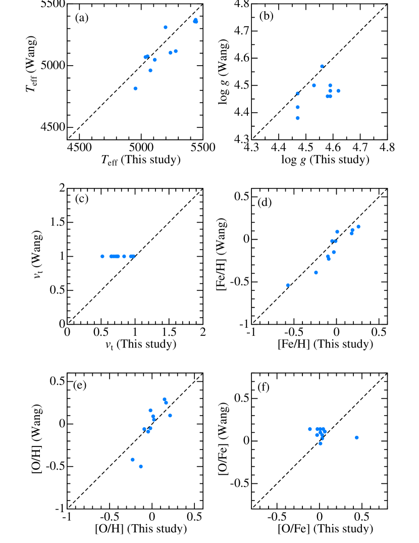
Figure 8: Comparison of the atmospheric parameters and the oxygen abundances derived in this study with those of Wang et al. (2009) for 11 field stars in common. (a) $T_{\rm eff}$, (b) $\log g$, (c) $v_{\rm t}$, (d) [Fe/H]. (e) [O/H], and (f) [O/Fe]. (Note that they assumed $v_{\rm t}=1$ km s^-1.)

It has been reported by several investigators that significant difficulties are involved in the spectroscopic analysis of lower main-sequence stars of late G to K-type (hereinafter we refer to this star group simply as “K dwarfs”). That is, the Fe abundances derived from lines of neutral and ionized stages (Fe i and Fe ii) are not consistent with each other (generally the latter is larger than the former), and this Fe ii vs. Fe i discrepancy becomes progressively more serious as the effective temperature ($T_{\rm eff}$) is lowered. See, e.g., Allende Prieto et al. (2004, cf. their Fig. 8); Kotoneva et al. (2006, cf. their Fig. 9), and Luck (2017, cf. his Fig. 1) for field stars; King & Schuler (2005; cf. their Fig. 4) for UMa moving group stars; Yong et al. (2004, cf. their Fig. 4) and Schuler et al. (2006b, cf. their Fig. 3) for Hyades cluster stars; Schuler et al. (2010; cf. their Fig. 1) for Pleiades cluster stars. Whichever reason is relevant for this trend (e.g., substantial non-LTE overionization effect related to stellar activity; cf. Takeda 2008), it must have a large impact if it is real, given the paramount importance of Fe lines in stellar spectroscopy. For example, the widely used method of determining the atmospheric parameters of solar-type stars based on Fe i and Fe ii lines (which makes use of the excitation equilibrium of Fe i and ionization equilibrium of Fe i/Fe ii; e.g., Takeda et al. 2002) would hardly be applicable to K dwarfs, since classical 1D plane-parallel model atmospheres would be no more valid for them.

However, some doubt still remains regarding whether this effect is really so important. Wang et al. (2009) carried out spectroscopic analysis of 30 nearby lower main-sequence stars at 4700 $\lesssim T_{\rm eff}\lesssim$ 5400 K. They could not confirm the appreciable $T_{\rm eff}$-dependent systematic discrepancy reported by Kotoneva et al. (2006), but found a reasonable consistency between Fe i and Fe ii abundances to a level of $\lesssim 0.1$ dex (cf. Fig. 5 therein). Furthermore, Aleo et al. (2017) conducted an extensive examination on this alleged “Fe abundance anomaly in K dwarfs” by carefully determining the Fe abundances from lines of neutral and ionized stages for 63 wide binary stars and 33 Hyades stars at 4300 $\lesssim T_{\rm eff}\lesssim$ 6100 K. Their important finding is the importance of line-blending effect for certain Fe ii lines, which becomes prominent for K dwarfs of lower $T_{\rm eff}$ where Fe ii lines are weaker while lines of neutral metals get stronger. By removing these lines, they found that the Fe ii–Fe i discrepancy is appreciably mitigated; e.g., for Hyades stars, only $\sim 0.1$ dex at 4500 K $\lesssim T_{\rm eff}$, though increasing to $\sim 0.3$ dex at further lower $T_{\rm eff}$ of $\sim 4300$ K (cf. Fig. 9 therein). Likewise, Tsantaki et al. (2019) very recently performed a detailed study on the Fe ionization equilibrium based on the spectra of 451 FGK-type stars (subsample of HARPS GTO planet survey program) and also arrived at the conclusion that unresolved line blending is probably the main reason for the apparent overabundance of Fe ii. They showed that $T_{\rm eff}$-independent consistent results could be obtained by rejecting suspicious Fe ii lines. These two recent investigations suggest that the considerably large Fe ii–Fe i disagreement reported in previous studies (e.g., as much as $\sim$ 0.5–0.6 dex at $T_{\rm eff}\sim 4500$ K for the case of Hyades K dwarfs; cf. Yong et al. 2004, Schuler et al. 2006b) is likely to be due to their inadequate choice of blending-affected Fe ii lines, leading to a significant overestimation of Fe ii abundances.

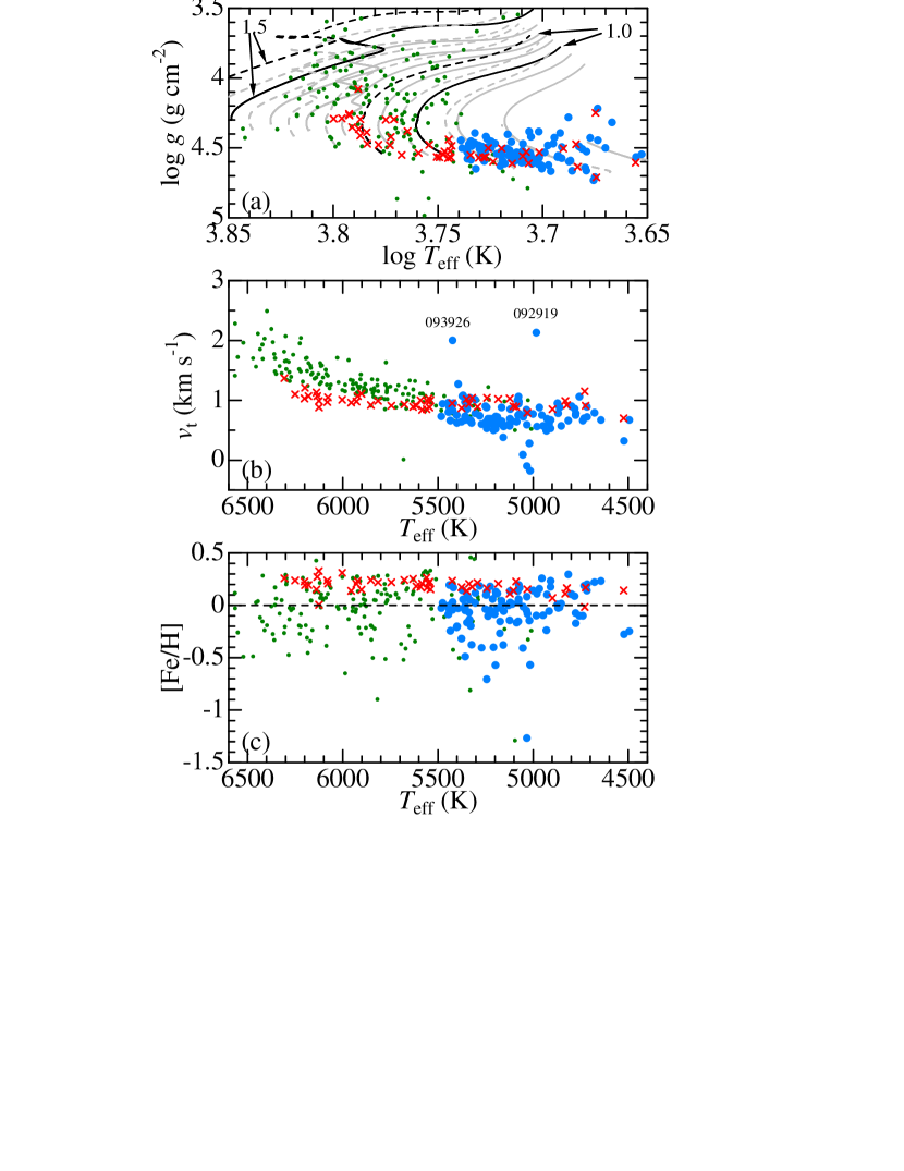
Figure 2: Spectroscopically determined $\log g$, $v_{\rm t}$, and [Fe/H] are plotted against $T_{\rm eff}$ in panels (a), (b), and (c), respectively. In panel (a) are also depicted the theoretical $\log g$ vs. $\log T_{\rm eff}$ relations corresponding to eight different masses (0.7, 0.8, 0.9, 1.0. 1.1, 1.2, 1.3, 1.4, and 1.5 $M_{\odot}$) for different metallicities ($z=0.01$ and $z=0.02$ in dashed and solid lines, respectively), which were taken from PARSEC stellar evolutionary tracks (Bressan et al. 2012, 2013). Apart from the program stars of this study (47 Hyades and 101 field stars shown by blue circles and red crosses respectively), 160 mid-F through early K dwarfs/subgiants investigated by Takeda et al. (2005) are also plotted in green dots for comparison.

This revelation reminded us of a similar problem related to oxygen abundance determination for K dwarfs. That is, the widely used high-excitation O i 7771–5 triplet lines tend to result in erroneously overestimated abundances (being progressively more serious with a decrease in $T_{\rm eff}$), which was reported in several studies on open cluster stars: UMa moving group (King & Schuler 2005; cf. their Fig. 4), M 34 as well as Pleiades (Schuler et al. 2004; cf. their Fig. 1 and Fig. 2), Hyades (Schuler et al. 2006a; cf. their Fig. 3), and NGC 752 (Maderak et al. 2013; cf. their Fig. 5). Actually, this effect of abundance anomaly they found was surprisingly large, because [O/H] values (oxygen abundance relative to the Sun) of K dwarfs derived from O i 7771–5 lines turned out to be unreasonably higher than those of G dwarfs by as much as $\lesssim 1$ dex, despite that they should have similar values for stars belonging to the same cluster.

Although their investigations were based on the assumption of LTE, the non-LTE effect evaluated in the standard manner using classical model atmospheres (see, e.g., Takeda 2003) can not explain this apparently large overabundance of [O/H], because non-LTE correction is strength-dependent and almost negligible for K dwarfs, where high-excitation O i 7771–5 lines are considerably weak because of lower $T_{\rm eff}$. So, if this is real, it might be due to some kind of non-classical activity-related phenomenon such as the intensification caused by chromospheric temperature rise (cf. Takeda 2008). However, in view of the similarity to the case of Fe abundance discrepancy (in the sense that considerably weak Fe ii and O i lines are involved for the anomalous abundances seen in K dwarfs), this problem on the reliability of O i 7771–5 triplet may be worth reinvestigation.

This situation motivated us to revisit these “spectroscopic K dwarf problems on Fe and O abundances” based on the spectral data for a large sample of G–K dwarfs (47 Hyades stars and 101 field stars). Our approach is simply to apply the standard method of analysis adopted in our previous studies to all these sample stars and see if any unreasonable result (such as suggesting the breakdown of classical modeling) comes out or not. More precisely, what we want to do and clarify in this investigation is as follows:

• We determine the atmospheric parameters of each program star in the conventional manner from the equivalent widths of Fe i and Fe ii lines while assuming the LTE (Saha–Boltzmann equation) as done by Takeda et al. (2005). If classical treatment is not valid for K dwarfs, the resulting parameters would reveal some kind of $T_{\rm eff}$-dependent inconsistency between G and K dwarfs. In this context, Hyades stars should play an especially important role, because their parameters are known to a sufficient precision. Comparison of our spectroscopically determined parameters and those already established by other methods would make a decisive touchstone.

• By using the model atmospheres corresponding to such determined atmospheric parameters, we then evaluate the oxygen abundance for each star by applying the spectrum-fitting method to O i 7771–5 (see, e.g., Takeda et al. 2015), where the non-LTE effect was taken into account according to Takeda’s (2003) calculation. Again, Hyades stars can serve as a good testbed, because they are considered to have practically the same O abundances. Are the resulting [O/H] values consistent with each other? Or do they show such considerable $T_{\rm eff}$-dependent disagreement as concluded by Schuler et al. (2006a)? This must be an interesting check. In addition, it is worthwhile to examine the behavior of [O/Fe] ($\equiv$[O/H]$-$[Fe/H]) ratios with a change in [Fe/H] (metallicity) obtained for field stars. Is the [O/Fe] vs. [Fe/H] diagram obtained from O i 7771–5 lines for K dwarfs consistent with that derived by Takeda & Honda (2005) for F–G stars with the same triplet? This can be another touchstone for judging the reliability of these high-excitation O i lines in context of oxygen abundance determination for K dwarfs.

2 OBSERVATIONAL DATA

As the target stars of this investigation, we adopted a sample of 148 dwarfs (consisting of 47 Hyades cluster stars and 101 field stars), which are in the apparent magnitude range of $V\sim$ 5–10. Regarding Hyades stars, since we intended to cover a rather wider range of spectral type (in order to clarify the $T_{\rm eff}$-dependence), main-sequence stars in the color range of $0.5\lesssim B-V\lesssim 1.2$ (corresponding to late F through mid K) were selected from de Bruijne et al.’s (2001) list. As to field stars, we mainly invoked Kotoneva et al.’s (2002) list of G–K dwarfs, from which 99 stars in the color range of $0.7\lesssim B-V\lesssim 1.2$ (corresponding to mid–late G through mid K) were chosen. In addition, in order to reinforce the sample of mid-K stars, 61 Cyg A and $\xi$ Boo B (both having $B-V\sim 1.2$) were also included. The basic data of these 148 stars are summarized in Table 1 (and in “tableE1.dat” of the online material). The $M_{V}$ vs. $B-V$ diagram for the program stars is shown in Figure 1a.

Our spectroscopic observations for 118 stars were done in 4 runs of 2010–2011 (2010 April/May, 2010 August, 2010 November/December, and 2011 November) by using the HIDES (HIgh Dispersion Echelle Spectrograph) placed at the coudé focus of the 188 cm reflector at Okayama Astrophysical Observatory. Equipped with three mosaicked 4K$\times$2K CCD detectors at the camera focus, HIDES enabled us to obtain an echellogram covering $\sim$ 5100–8800 $\rm\AA$ with a resolving power of $R\sim 67000$. The observations for the remaining 30 stars were done on 2014 September 9 with the HDS (High Dispersion Spectrograph) placed at the Nasmyth platform of the 8.2-m Subaru Telescope, by which high-dispersion spectra with a resolution of $R\simeq 80000$ covering $\sim$ 5100–7800 $\rm\AA$ (with two 4K$\times$2K CCDs) were obtained. The observed dates for each of the program stars are given in “tableE1.dat”.

The reduction of the spectra (bias subtraction, flat-fielding, scattered-light subtraction, spectrum extraction, wavelength calibration, and continuum normalization) was performed by using the “echelle” package of the software IRAF in a standard manner. If a few consecutive exposures were done for a star in a night, we co-added these to improve the signal-to-noise ratio. The average S/N of the finally resulting spectrum is typically $\sim$ 100–300 for most cases.

3 STELLAR PARAMETERS

3.1 Atmospheric Parameters Based on Fe Lines

The four parameters [$T_{\rm eff}$ (effective temperature), $\log g$ (logarithmic surface gravity), $v_{\rm t}$ (microturbulent velocity dispersion), and [Fe/H] (Fe abundance relative to the Sun)] were spectroscopically determined from the equivalent widths ($W_{\lambda}$) of Fe i and Fe ii lines based on the principle and algorithm described in Takeda et al. (2002), which requires that (i) Fe i abundances do not depend upon $\chi_{\rm low}$ (lower excitation potential), (ii) mean Fe i and Fe ii abundances are equal, and (iii) Fe i abundances do not depend upon $W_{\lambda}$, while assuming that LTE Saha–Boltzmann equation holds.

The measurement of $W_{\lambda}$ for each Fe line (selected from the line list of Takeda et al. 2005) was done by the Gaussian-fitting method in most cases (though special function constructed by convolving the rotational broadening function with the Gaussian function was used for several cases of appreciably large rotational velocity). In order to avoid measuring inadequate lines affected by blending, we carried out measurements on the computer display, while comparing the stellar spectrum with Kurucz et al’s (1984) solar spectrum and examining the theoretical strengths of neighborhood lines computed with the help of Kurucz & Bell’s (1995) atomic line data.

Practically, we applied the program TGVIT (Takeda et al. 2005; cf. Sect. 2 therein), to the measured $W_{\lambda}$’s of Fe i and Fe ii lines. As done in Takeda et al. (2005), we restricted to using lines satisfying $W_{\lambda}\leq 100$ m$\rm\AA$ and those showing abundance deviations from the mean larger than $2.5\sigma$ were rejected. The typical numbers of finally adopted lines are 72–235 (mean = 208) for Fe i and 5–22 (mean = 14) for Fe ii (number of available lines is smaller for stars showing broader lines). The resulting final parameters are presented in Table 1 and “tableE1.dat”. The internal statistical errors (cf. Section 3.2 of Takeda et al. 2002) involved with these solutions are in the range of 10–85 K (mean = 24 K) for $T_{\rm eff}$, 0.02–0.26 dex (mean = 0.06 dex) for $\log g$, 0.1–0.5 km s^-1 (mean = 0.2 km s^-1) for $v_{\rm t}$, and 0.01–0.07 dex (mean = 0.03 dex) for [Fe/H]. The detailed data of $W_{\lambda}$ and $A$(Fe) (Fe abundances corresponding to the final solutions) for each star are given in “tableE2.dat” of the online material.

3.2 Trends and Mutual Correlations

These spectroscopically determined $T_{\rm eff}$ values are plotted against $B-V$ and $M_{V}$ in Figures 1b and 1c, where we can see that they are well correlated with each other. The color-dependence of [Fe/H] depicted in Figure 1d indicates the near-constancy of [Fe/H] for Hyades stars and a tendency of decreasing [Fe/H] towards a bluer $B-V$ for field stars (consistent with Fig. 8 of Kotoneva et al. 2002). Figure 1e shows the comparison of our spectroscopic [Fe/H] with the photometric metallicity ([Fe/H]^photo) determined by Kotoneva et al. (2002) based on the position in the color–magnitude diagram, which shows a reasonable correlation between these two (though their [Fe/H]^photo tends to be somewhat lower).

In Figures 2a–2c are plotted $\log g$, $v_{\rm t}$, and [Fe/H] against $T_{\rm eff}$, where the results of 160 dwarfs/subgiants (of mostly F–G type) determined by Takeda et al. (2005) are also shown for comparison. We can see from Figure 2a (where theoretical $\log g$ vs. $\log T_{\rm eff}$ relations are also depicted) that most of our program stars occupy consistent positions as main-sequence stars. However, deviations (i.e., underestimation of $\log g$) begins to appear towards low $T_{\rm eff}$ end, which means that precision of $\log g$ tends to gradually deteriorate as $T_{\rm eff}$ is lowered below $\lesssim 5000$ K. (see Section 5.1).

Regarding microturbulence, meaningless negative $v_{\rm t}$ values were obtained for two considerably metal-poor stars HIP 057939 ($-0.10$ km s^-1) and HIP 098792 ($-0.18$ km s^-1), which is due to the result of extrapolation. In actual determination of oxygen abundance (cf. Section 4), we tentatively assigned $v_{\rm t}=0.5$ km s^-1 for these stars. We also note that two stars (HIP 093926, HIP 092919) show anomalously high $v_{\rm t}$ values ($\sim 2$ km s^-1), which must be related to the fact that these stars show exceptionally broad lines indicative of higher rotation. It is interesting to note in Figure 2b that, while the $v_{\rm t}$ results determined for 101 field stars (blue circles) tend to decrease as $T_{\rm eff}$ is lowered as a natural continuation of the trend derived by Takeda et al. (2005) (represented by green dots), those obtained for 47 Hyades stars (red crosses) appear to be almost independent upon $T_{\rm eff}$ and nearly flat at $\sim 1$ km s^-1. This may suggest a possibility that $v_{\rm t}$ could be somehow influenced by stellar age or activity, because Hyades stars are comparatively younger and of higher activity.

Figure 2c shows that the metallicities of Hyades stars are nearly constant at [Fe/H] $\sim 0.2$; i.e., the mean ($\pm$ standard deviation) is $\langle$[Fe/H]$\rangle$ = 0.19 ($\pm 0.07$). This is slightly higher than the value of $\langle$[Fe/H]$\rangle$ = 0.11 ($\pm 0.08$) derived for F–G dwarfs by Takeda et al. (2013), but consistent within permissible limits in view of the fact that the published values of Hyades metallicity range at $0.1\lesssim$ [Fe/H] $\lesssim 0.2$.

Meanwhile, those for field G–K stars range mostly from $-0.7$ to $+0.3$ (like the case of 160 sample stars studied by Takeda et al. 2005), though only HIP 057939 is distinctly metal-deficient ([Fe/H] = $-1.27$) compared to the others. In connection with metallicity, it may be worth examining the population of our program stars. For this purpose, their kinematic parameters were computed by following the same procedure as adopted in Takeda (2007; cf. Sect. 2.2 therein), where the necessary data (equatorial coordinates, parallax, proper motions, and radial velocity) were taken from those of Gaia DR2 (Gaia Collaboration et al. 2016, 2018) published as CDS/ADC Collection of Electronic Catalogues (No. 1345, 0, 2018) and available via SIMBAD. The resulting orbital parameters and space velocity components relative to the Local Standard of Rest (LSR) are given in tableE1.dat of the online material. The $z_{\rm max}$ (maximum separation from the galactic plane) vs. $V_{\rm LSR}$ (rotation velocity component) diagram usable for discriminating stellar population is displayed in Figure 3a, which indicates that most of our target stars belong to the thin disk population (with a few exceptions such as HIP 057939 and HIP 082588 which may be of thick-disk population). Figure 3b illustrates the correlation between the space velocity $|v_{\rm LSR}|$ ($\equiv\sqrt{U_{\rm LSR}^{2}+V_{\rm LSR}^{2}+W_{\rm LSR}^{2}}$), and metallicity ([Fe/H]). Though the scatter is rather large, we can recognize that $|v_{\rm LSR}|$ tends to increase with a decrease in [Fe/H] as expected It can also be seen that those two stars of apparent thick-disk population mentioned above show distinctly larger $|v_{\rm LSR}|$ (especially HIP 057939).

4 OXYGEN ABUNDANCE DETERMINATION

4.1 Spectrum-Fitting Analysis

We determine the oxygen abundances of 148 target stars from the O i 7771–5 triplet feature as done in previous studies (e.g., Takeda et al. 2015). Based on the atmospheric parameters determined in Section 3.1, the model atmosphere for each star was constructed by interpolating Kurucz’s (1993) ATLAS9 model grid. We similarly evaluated the non-LTE departure coefficients for O corresponding to each model by interpolating the grid computed by Takeda (2003).

Abundance determination was carried out by using the spectrum-fitting technique as done in Takeda et al. (2015), which establishes the most optimum solutions accomplishing the best match between theoretical and observed spectra by using the numerical algorithm described in Takeda (1995), while simultaneously varying the abundances of relevant key elements ($A_{1}$, $A_{2}$, $\ldots$), the macrobroadening parameter ($v_{\rm M}$), and the radial-velocity (wavelength) shift ($\Delta\lambda$).

We selected 7770–7782 Å as the wavelength region for fitting, which includes O i 7771–5 triplet lines and Fe i 7780 line as the conspicuous lines. Regarding the atomic data of spectral lines, the same values as used in Takeda et al. (2015) were used unchanged for 3 lines of O i 7771–5 triplet and 6 lines of CN molecules (cf. Table 2 therein). Otherwise, we invoked the data compiled in the VALD database (Ryabchikova et al. 2015) for all lines included in this region (for example. $\log gf=+0.03$ was adopted for the strong Fe i 7780.556 line of $\chi_{\rm low}$ = 4.47 eV). We varied only $A$(O) and $A$(Fe) for the abundances to be adjusted, while other elemental abundances (necessary for computing the background spectrum in this region) were fixed at the metallicity-scaled values. The non-LTE effect was taken into account for the O i 7771–5 lines. Since the OAO/HIDES spectrum often suffers defects due to bad columns of CCD in this region, we had to mask them occasionally. The convergence of the solutions turned out fairly successful for all cases. How the theoretical spectrum for the converged solutions fits well with the observed spectrum for each star is displayed in Figure 4 (Hyades stars) and Figure 5 (field stars).

4.2 Abundance-Related Quantities

Next, with the help of Kurucz’s (1993) WIDTH9 program (which had been considerably modified in various respects; e.g., inclusion of non-LTE effects, etc.), we computed the equivalent widths ($W_{7772}$, $W_{7774}$, and $W_{7775}$) of three O i triplet lines (at 7771.944, 7774.166, and 7775.388 Å) inversely from the non-LTE abundance solution $A^{\rm N}$(O) (resulting from fitting analysis) along with the adopted atmospheric model and parameters. Based on these $W$ values, the non-LTE ($A^{\rm N}$: essentially the same as the fitting solution) and LTE ($A^{\rm L}$) oxygen abundances were then derived, from which the corresponding non-LTE corrections could be obtained as $\Delta\equiv A^{\rm N}-A^{\rm L}$. In Table 1 (and also in “tableE1.dat”) are presented [O/H] $(\equiv A^{\rm N}-8.861)$, $W_{7774}$, $\Delta_{7774}$ (for the middle line of the triplet)

In order to estimate abundance errors caused by uncertainties in atmospheric parameters, we derived six kinds of abundance variations ($\delta_{T+}$, $\delta_{T-}$, $\delta_{g+}$, $\delta_{g-}$, $\delta_{v+}$, and $\delta_{v-}$) for $A^{\rm N}$ by repeating the analysis on the $W_{7774}$ values while perturbing the standard atmospheric parameters interchangeably by $\pm 100$ K in $T_{\rm eff}$, $\pm 0.1$ dex in $\log g$, and $\pm 0.5$ km s^-1 in $v_{\rm t}$ (which are larger than the internal statistical errors described in Section 3.1 but tentatively chosen by considering possible systematic errors; cf. Section 5.1).

Errors ($\delta W$) due to random noises in the equivalent widths ($W$) were also estimated by invoking the relation derived by Cayrel (1988) corresponding to the S/N ratio ($\sim$ 100–200) measured for each star’s spectrum in the neighborhood of O i triplet. We then evaluated the abundances for each of the perturbed $W_{+}(\equiv W+\delta W)$ and $W_{-}(\equiv W-\delta W)$, from which the differences from the standard abundance ($A$) were derived as $\delta_{W+}(>0)$ and $\delta_{W-}(<0)$.

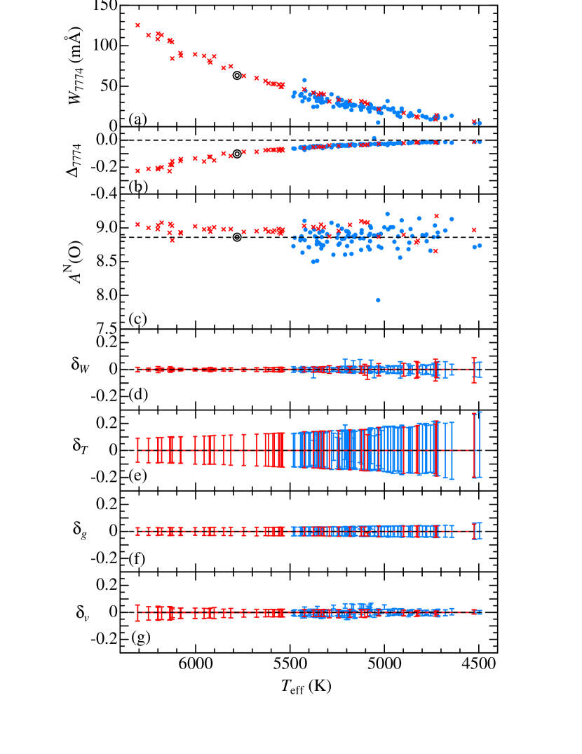
Figure 6: Oxygen abundance and related quantities plotted against $T_{\rm eff}$. (a) $W_{7774}$ (equivalent width of O i 7774.166), (b) $\Delta_{7774}$ (non-LTE correction for O i 7774.166), (c) $A^{\rm N}$(O) (non-LTE oxygen abundance derived from spectrum fitting). (d) $\delta_{W+}$ and $\delta_{W-}$ (abundance change corresponding to perturbation of $+\delta W$ and $-\delta W$, where $\delta W$ is the uncertainty of equivalent width evaluated according to Cayrel 1988). (e) $\delta_{T+}$ and $\delta_{T-}$ (abundance variations in response to $T_{\rm eff}$ changes of +100 K and $-100$ K), (f) $\delta_{g+}$ and $\delta_{g-}$ (abundance variations in response to $\log g$ changes by $+0.1$ dex and $-0.1$ dex), and (g) $\delta_{v+}$ and $\delta_{v-}$ (abundance variations in response to perturbing the $v_{\rm t}$ value by +0.5 km s^-1 and $-$0.5 km s^-1). Note that the signs of these $\delta$ values are $\delta_{W+}>0$, $\delta_{W-}<0$, $\delta_{T+}<0$, $\delta_{T-}>0$, $\delta_{g+}>0$, $\delta_{g-}<0$, $\delta_{v+}<0$ and $\delta_{v-}>0$. The non-LTE solar O abundance of 8.861 derived in the similar manner (cf. Takeda et al. 2015) is indicated by the horizontal dashed line in panel (c). The large double circles in panels (a)–(c) denote the solar values (cf. footnote 7). Otherwise, the same meanings of the symbols (and their colors) as in Figure 1.

These $W_{7774}$, $\Delta_{7774}$, $A^{\rm N}$(O), $\delta_{W\pm}$, $\delta_{T\pm}$, $\delta_{g\pm}$, and $\delta_{v\pm}$ are plotted against $T_{\rm eff}$ in panels (a)–(g) of Figure 6, respectively, from which the following trends can be read.

• It can be seen that $W_{7774}$ progressively decreases as $T_{\rm eff}$ is lowered, reflecting that the occupation number in the highly-excited lower level ($\chi_{\rm low}=9.15$ eV) of this transition is quite $T_{\rm eff}$-sensitive ($\propto 10^{-5040\chi_{\rm low}/T_{\rm eff}}$).

• Likewise, $|\Delta_{7774}|$ (absolute value of negative non-LTE correction) declines with decreasing $T_{\rm eff}$, because of the close connection between $\Delta$ and $W$ (cf. Takeda 2003) for the O i 7771–5 triplet. Accordingly, while non-LTE correction is still appreciable for late F–early G dwarfs ($\sim$ 0.1–0.2 dex), it becomes practically negligible for K dwarfs of $T_{\rm eff}\lesssim 5000$ K.

• The oxygen abundances ($A^{\rm N}$) do not show any clear $T_{\rm eff}$-dependence for both Hyades and field stars. While the former are nearly constant on average (though the scatter grows at $T_{\rm eff}\lesssim 5000$ K), the latter are diversified mostly in the range of $\sim$ 8.5–9.2.

• The mean of [O/H] for 47 Hyades stars is $\langle$[O/H]$\rangle$ = 0.11 ($\pm 0.09$), Although this is slightly lower than the value ($\langle$[O/H]$\rangle$ = 0.22 $\pm 0.14$) derived by Takeda et al. (2013) for Hyades F–G dwarfs from O i 6156–8 lines, we consider that both are reasonably consistent within the allowable range (see Sect. 1 of Takeda et al. 2013 for a summary of published [O/H] values in various literature).

• Among the various sources of abundance errors, most important is $\delta_{T\pm}$ (ranging from $\sim$ 0.1 dex to $\sim 0.2$ dex or even more; especially large around lowest $T_{\rm eff}$) reflecting the high-excitation nature of O i triplet lines, while $\delta_{W\pm}$, $\delta_{g\pm}$ and $\delta_{v\pm}$ are comparatively insignificant (only several hundredths dex).

5 DISCUSSION

5.1 Reliability of Spectroscopic Parameters

As to whether stellar parameters of K dwarfs can be reliably determined based on Fe i and Fe ii lines, which was the first aim of this study (under the suspicion that LTE ionization equilibrium of Fe i/Fe ii may break down), we can examine this problem by comparing the $T_{\rm eff}$ and $\log g$ values of Hyades dwarfs spectroscopically derived in Section 3.1 with those of de Bruijne et al. (2001), who made use of the theoretical color–magnitude relations along with the well-established luminosities from Hipparcos parallaxes. These comparisons are illustrated in Figure 7.

Figure 7a suggests that a rather satisfactory agreement is observed for $T_{\rm eff}$, though $T_{\rm eff}$(This study) tends to be is slightly higher than $T_{\rm eff}$(de Bruijne) by $\lesssim 100$ K (Figure 7c). The average $\langle\Delta T_{\rm eff}$(de Bruijne$-$This study)$\rangle$ is $-67(\pm 50)$ K. Regarding $\log g$, we can see a tendency of $\log g$(This study) being smaller than $\log g$(de Bruijne) (Figure 7b). However, excepting two stars (HIP 20762 and HIP 25639) the difference is within $\lesssim$0.1–0.2 dex (Figure 7d). The average $\langle\Delta\log g$(de Bruijne$-$This study)$\rangle$ is $+0.06(\pm 0.09)$ dex (for all stars) or $+0.05(\pm 0.06)$ dex (excluding two outliers). These $\Delta T_{\rm eff}$ and $\Delta\log g$ show a weak correlation (Figure 7e) which is presumably because higher $T_{\rm eff}$ (enhancing ionization) is compensated by higher $\log g$ (suppressing ionization).

Considering the results of this test using Hyades G–K stars, we may conclude that our spectroscopically determined $T_{\rm eff}$ and $\log g$ do not suffer significant errors, which are determinable based on Fe i and Fe ii lines to typical precisions of $\lesssim 100$ K and $\lesssim 0.1$ dex under the assumption of LTE Saha–Boltzmann equation. Admittedly, the tendency of slightly higher $T_{\rm eff}$ and lower $\log g$ in our spectroscopic parameters may indicate a possibility of marginal overionization. However, since $\Delta T_{\rm eff}$ as well as $\Delta\log g$ do not show any conspicuous dependence upon $T_{\rm eff}$, we can rule out the possibility of significant $T_{\rm eff}$-dependent Fe i–Fe ii discrepancy progressively increasing towards lower $T_{\rm eff}$. In this regard, our result is in favor of Aleo et al.’s (2017) conclusion that such previously alleged considerable discordance between Fe i and Fe ii abundances in K dwarfs is largely due to improper inclusion of blended Fe ii lines and practically insignificant ($\lesssim 0.1$ dex) as long as stars of $T_{\rm eff}\gtrsim 4500$ K are concerned. We should note, however, that lowering of the precision is more or less unavoidable at the low $T_{\rm eff}$ regime (see Section 3.2 in connection with the trend of $\log g$ vs. $T_{\rm eff}$ in Figure 2a), because Fe ii lines are so weakened that their measurements must suffer larger uncertainties.

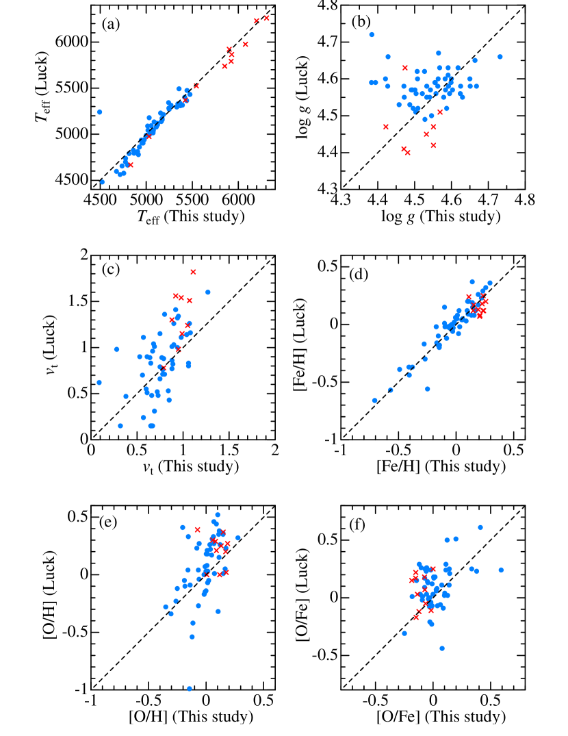
Figure 10: Comparison of the atmospheric parameters and the oxygen abundances derived in this study with those of Luck (2017) for 55 field stars and 11 Hyades stars in common. Otherwise, the same as in Figure 8.

It may be worth comparing the spectroscopic parameters with those determined by other methods in recent representative studies. The comparisons with the results of Wang et al. (2009), Ramírez et al. (2013), and Luck (2017) are shown in Figures 8, 9, and 10, respectively. In all three investigations, $T_{\rm eff}$ was determined photometrically from colors, $\log g$ by comparing the position on the $\log L$ vs. $\log T_{\rm eff}$ diagram ($L$: stellar luminosity) with stellar evolutionary tracks, and $v_{\rm t}$ by requiring that the resulting abundances from Fe i lines do not show any systematic correlation with line strengths (though $v_{\rm t}=1$ km s^-1 was assumed by Wang et al. 2009). We can read the following characteristic trends from these figures.

• Our spectroscopic $T_{\rm eff}$ is satisfactorily consistent with the photometrically determined values of all three studies (Figures 8a, 9a, and 10a).

• Since the range of $\log g$ is rather narrow in G–K dwarfs (unlike the case of $T_{\rm eff}$), our spectroscopic $\log g$ does not appear to be well correlated with the values based on the theoretical HR diagram. However, the differences themselves are not so large, which are mostly within $\lesssim$ 0.1–0.2 dex. We see on average that $\log g$(Wang) (Figure 8b) tends to be somewhat lower, while $\log g$(Ramírez) (Figure 9b) and $\log g$(Luck) (Figure 10b) somewhat higher, as compared with our $\log g$ derived from Fe i and Fe ii lines.

• Regarding $v_{\rm t}$, while Ramírez et al.’s (2013) results are almost consistent with our determination (Figure 9c), those of Luck (2017) show some systematic trend (Figure 10c) that they tend to be larger for higher $v_{\rm t}$ (while somewhat smaller for lower $v_{\rm t}$). We can see from Figure 8c that $v_{\rm t}=1$ km s^-1 assumed by Wang et al. (2009) was not so a bad choice.

• As to [Fe/H], a good agreement is confirmed with all these studies (cf. Figures 8d, 9d, and 10d).

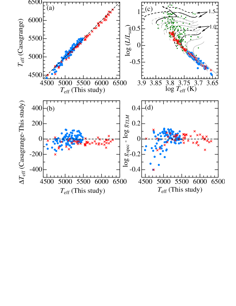
Figure 11: Panels (a) and (b) illustrate the comparison of the photometric $T_{\rm eff}$ derived from $B-V$ and [Fe/H] by using Casagrande et al.’s (2010) formula with the spectroscopic $T_{\rm eff}$ adopted in this study: (a) $T_{\rm eff}$(Casagrande) vs. $T_{\rm eff}$(This study) and (b) $T_{\rm eff}$(Casagrande)$-T_{\rm eff}$(This study) vs. $T_{\rm eff}$(This study). In panel (c) is shown the $L$(bolometric luminosity) vs. $T_{\rm eff}$ relation for the program stars, where the theoretical PARSEC tracks are also depicted similarly to Figure 2a. The differences between $\log g_{\rm spec}$ (spectroscopic surface gravity adopted in this study) and $\log g_{TLM}$ (theoretical surface gravity derived from $T_{\rm eff}$, $L$, and $M$) are plotted against $T_{\rm eff}$ in panel (d). See the caption of Figure 2 for the meanings of the symbols and lines.

As another check for the spectroscopic $T_{\rm eff}$ adopted in this study, we also computed the photometric $T_{\rm eff}$ from $B-V$ and [Fe/H] by using Casagrande et al.’s (2010) calibration based on the infrared flux method. The comparisons between $T_{\rm eff}$(This study) and $T_{\rm eff}$(Casagrande) are shown in Figures 11a and 11b, where we can recongize that both are in satisfactory agreement.

It is also worthwhile to examine how our adopted spectroscopic $\log g_{\rm spec}$ is compared with the direct value ($\log g_{TLM}$) derived from $T_{\rm eff}$, $L$ (bolometric luminosity), and $M$ (mass). The $L$ values were derived from $V$ (apparent magnitude; cf. Table 1), Gaia DR2 parallax (taken from the SIMBAD database; see also Section 3.2), and the bolometric correction evaluated by interpolating Alonso et al.’s (1995) Table 4. Then, $M$ for each star was evaluated from its position on the $\log L$ vs. $\log T_{\rm eff}$ diagram (cf. Figure 11c) by comparing the theoretical PARSEC tracks (Bressan et al. 2012, 2013), where fine grids are available with a step of 0.005 $M_{\odot}$ over a wide metallicity range from $z=0.0001$ to $z=0.06$ (we regard $z=z_{\odot}\times 10^{{\rm[Fe/H]}}$ as the stellar metallicity where $z_{\odot}=0.014$). The difference between $\log g_{\rm spec}$ and the resulting $\log g_{TLM}$ is plotted against $T_{\rm eff}$ in Figure 11d, which suggests that both are mostly consistent within $\sim\pm 0.1$ dex (though several $\log g_{\rm spec}$ values are appreciably underestimated at $T_{\rm eff}\lesssim 5000$ K; see also Figure 2a). These $\log L$, $M$, and $\log g_{TLM}$ values determined for each star are given in “tableE1.dat” of the online material.

5.2 Oxygen Abundance from O I 7771–5

We go on to discussing the second subject of this study: whether or not credible oxygen abundances of K dwarfs can be derived from the high-excitation O i triplet lines at 7771–5 Å, for which unreasonably high abundances were reported by Schuler et al.’s group in their studies on open clusters (cf. Section 1). As was the case for stellar parameters, Hyades G–K dwarfs can serve as an important touchstone in this respect, because they should retain almost the same (primordial) oxygen abundances in their photospheres.

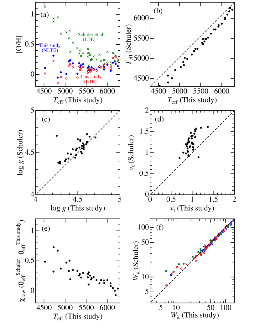
Figure 12: Comparison of the our oxygen abundances and atmospheric parameters derived for Hyades stars with those of Schuler et al. (2006a) (37 stars are in common). (a) [O/H] values plotted against $T_{\rm eff}$(ours), where [O/H](theirs, LTE), [O/H](ours, NLTE), ad [O/H](ours, LTE) are denoted by green crosses, blue filled circles, and red open circles, respectively. (b) $T_{\rm eff}$(theirs) vs. $T_{\rm eff}$(ours). (c) $\log g$(theirs) vs. $\log g$(ours). (d) $v_{\rm t}$(theirs) vs. $v_{\rm t}$(ours). (e) Differences of $\chi_{\rm low}\theta_{\rm eff}$(theirs)$-$$\chi_{\rm low}\theta_{\rm eff}$(ours) (which defines the shift in the abscissa of curve of growth) plotted against $T_{\rm eff}$(ours), where $\chi_{\rm low}$ = 9.146 eV (lower excitation potential of the O i 7771–5 triplet), and $\theta_{\rm eff}\equiv 5040/T_{\rm eff}$ ($T_{\rm eff}$ in K). (f) $W$(theirs) vs. $W$(ours) diagram, where blue open circles, green filed circles, and red crosses correspond to O i 7771.944, 7774.166, and 7775.388 lines, respectively.

Schuler et al. (2006a) derived a markedly increasing [O/H](LTE) for Hyades dwarfs with a decrease in $T_{\rm eff}$; i.e., $\sim+0.2$ (at $T_{\rm eff}\sim$ 6000–5500 K), $\sim+0.5$ (at $T_{\rm eff}\sim 5000$ K), and $\sim+1.0$ (at $T_{\rm eff}\sim 4500$ K) as shown in their Fig. 3. Their values are reproduced in Figure 12a (crosses) for 37 stars in common with our sample. However, our results for Hyades stars turned out markedly different from theirs as manifestly seen from Figure 12a, where [O/H](NLTE) and [O/H](LTE) (represented by filled and open symbols, respectively) are plotted against $T_{\rm eff}$. That is, our [O/H] values do not show any such progressive increase towards lower $T_{\rm eff}$ as reported by Schuler et al. (2006a) but distribute around $\sim+0.2$, being consistent with the expectation that these stars should show similar oxygen abundances.

We investigated the cause of this discrepancy by comparing the adopted stellar parameters in both studies. Comparisons of $T_{\rm eff}$, $\log g$, and $v_{\rm t}$ are illustrated in Figures 12b, 12c, and 12d, respectively. It is apparent from Figure 12b that a considerable disagreement exists between Schuler et al.’s $T_{\rm eff}$ (photometric determination using colors) and our $T_{\rm eff}$ (spectroscopic determination from Fe lines) in the sense that the former is systematically lower by several hundred K and the difference progressively increasing towards lower $T_{\rm eff}$. Meanwhile, a more or less reasonable consistency (excepting an outlier) is observed for $\log g$ (Figure 12c), which they derived from theoretical evolutionary tracks. As to $v_{\rm t}$, Schuler et al.’s values tend to be somewhat higher than ours especially in the regime of larger $v_{\rm t}$ or higher $T_{\rm eff}$ (Figure 12d). This disagreement may be explained by the fact that they used Allende Prieto et al.’s (2004) empirical formula derived for field stars and that our $v_{\rm t}$ values derived for Hyades dwarfs tends to be lower than those of field dwarfs at $T_{\rm eff}\gtrsim 5500$ K as remarked in Section 3.2 (cf. Figure 2b).

In view of these results along with the parameter-dependence of the abundances discussed in Section 4.2, it must be the difference in $T_{\rm eff}$ that is mainly responsible for the considerable discrepancy in [O/H] between Schuler et al. (2006a) and this study, because the oxygen abundance from high-excitation O i 7771–5 triplet is highly sensitive to a change in $T_{\rm eff}$ (Figure 6e) while the roles played by $\log g$ and $v_{\rm t}$ are insignificant (Figures 6f and 6g). This can be confirmed from Figure 12e, where $\chi_{\rm low}\theta_{\rm eff}$(Schuler)$-$$\chi_{\rm low}\theta_{\rm eff}$(This study) ($\theta_{\rm eff}\equiv 5040/T_{\rm eff}$; this is the expected abundance variation for neutral oxygen of dominant population due to the difference in $T_{\rm eff}$) is plotted against $T_{\rm eff}$ for each star. We can see from this figure that the abundance change systematically grows with a decrease in $T_{\rm eff}$ (from $\sim$ 0.1–0.2 dex at $T_{\rm eff}\sim 6000$ K up to $\sim 0.6$ dex at $T_{\rm eff}\sim 4500$ K), which reasonably explains why Schuler et al.’s [O/H] values tend to be progressively larger than ours towards lower $T_{\rm eff}$. Besides, we found that the equivalent widths of the O i triplet lines measured by them and used for their analysis tend to be somewhat overestimated (by several tens %) for weak lines ($W_{\lambda}\lesssim 20~{}$mÅ) in comparison with our values (Figure 12f), though both are consistent for lines of medium strength. This would have further enhanced the overestimation of their [O/H] in case of such small $W_{\lambda}$ (i.e., $T_{\rm eff}\lesssim 5000$ K). As such, we consider that Schuler et al.’s (2006a) anomalous [O/H] results derived for Hyades dwarfs (conspicuously increasing towards lower $T_{\rm eff}$) are mainly due to their inadequate $T_{\rm eff}$ scale (i.e., too low by several hundred K) and thus should not be seriously taken.

The results of this study suggest that consistent oxygen abundances for Hyades G–K dwarfs (i.e., without showing any systematic trend in terms of $T_{\rm eff}$) can be derived even based on the high-excitation O i 7771–5 triplet lines. The mean non-LTE $\langle$[O/H]$\rangle$ for 37 stars (common to Schuler et al.) depicted in Figure 12a is $+0.12$ ($\sigma=0.09$), and that for all our 47 Hyades stars (cf. Figure 6c) is identically $+0.12$ ($\sigma=0.09$), which are favorably compared (i.e., within error bars) with $\langle$[O/H]$\rangle=+0.22(\pm 0.14)$ obtained by Takeda et al. (2013) for Hyades F–G stars based on O i 6156–8 lines.

Even so, it should be kept in mind that precision of abundance determination would naturally deteriorate for K dwarfs ($T_{\rm eff}\lesssim 5000$ K) because the strengths of these high-excitation O i triplet lines are considerably weakened, which makes measurement more difficult (e.g. due to increased importance of blending by other lines). This can be manifestly seen from the appreciable scatter of [O/H] at $T_{\rm eff}\lesssim 5000$ K in Figure 12a. Yet, we would like to stress that such significant “$T_{\rm eff}$-dependent systematic trend” as reported by Schuler et al. (2006a) is unlikely.

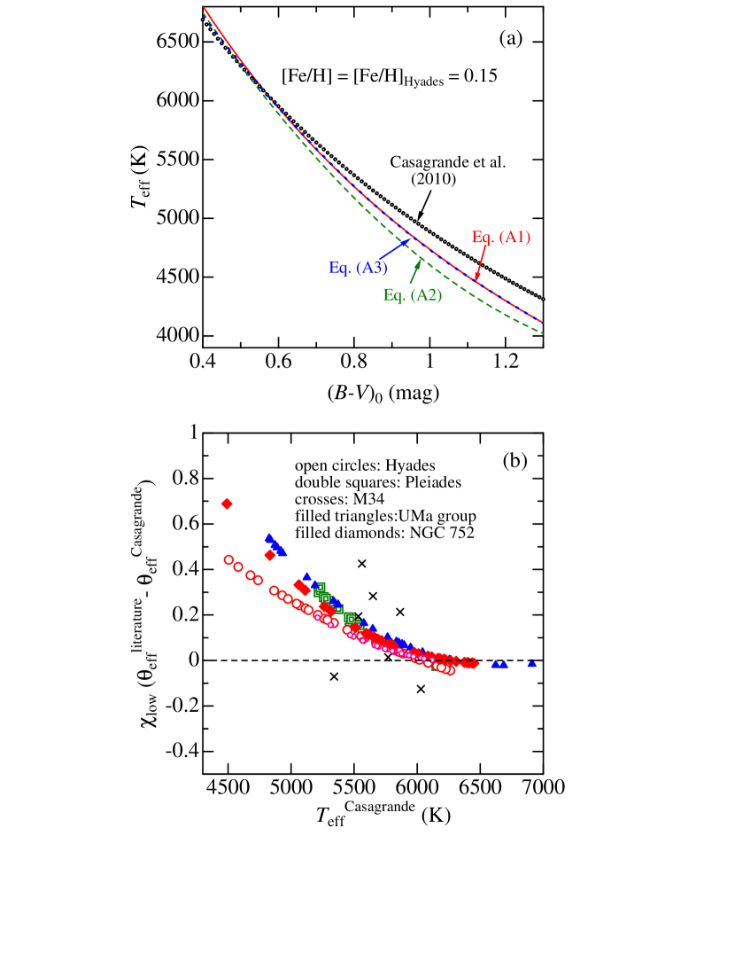
Figure 14: (a) Comparison of three $T_{\rm eff}$ vs. $B-V$ relations (lines) used in previous studies on the [O/H] trends of open cluster stars (cf. Table 2) with that of Casagrande et al. (2010) (black filled circles), where [Fe/H] is set at +0.15 (= [Fe/H]_Hyades) for all cases. Red solid line — Equation (A1), green dashed line — Equation (A2), and blue dotted line — Equation (A3). (b) Differences of $\chi_{\rm low}\theta_{\rm eff}$(literature)$-$$\chi_{\rm low}\theta_{\rm eff}$(Casagrande) (see the caption of Figure 12e for the meanings of $\theta_{\rm eff}$ and $\chi_{\rm low}$) are plotted against $T_{\rm eff}$(Casagrande), where $T_{\rm eff}$(literature) is the actual value used by the relevant study and $T_{\rm eff}$(Casagrande) was calculated according to Casagrande et al. (2010) along with each star’s $B-V$ and cluster [Fe/H]. Large open circles — Hyades (SCH06), small open circles — Hyades (MAD13), double squares — Pleiades (SCH04), crosses — M 34 (SCH04), filled triangles — UMa moving group (KS05), and filled diamonds — NGC 752 (MAD13). (See the caption of Table 2 for the key to the reference code.) Note that the colors of the symbols are so chosen as to match those of the lines in panel (a) corresponding to the $T_{\rm eff}$ vs. $B-V$ formula adopted in each paper.

Admittedly, what has been argued above is specific to Hyades dwarfs and we can not say much about the $T_{\rm eff}$-dependent anomaly in [O/H] derived from O i 7771–5 (i.e., progressively increasing towards lower $T_{\rm eff}$) also reported for other cluster stars: e.g., UMa moving group (King & Schuler 2005); Pleiades and M 34 (Schuler et al. 2004); NGC 752 (Maderak et al. 2013). We consider, however, that almost the same argument may also apply to the consequences of these studies, because we confirmed that the $T_{\rm eff}$ scale they adopted tends to be systematically lower as compared with that of Casagrande et al. (2010) (which is consistent with our spectrooscopic $T_{\rm eff}$; cf. Figures 11a and 11b). The details of this examination are separately described in Appendix A (see also Table 2 and Figure 14).

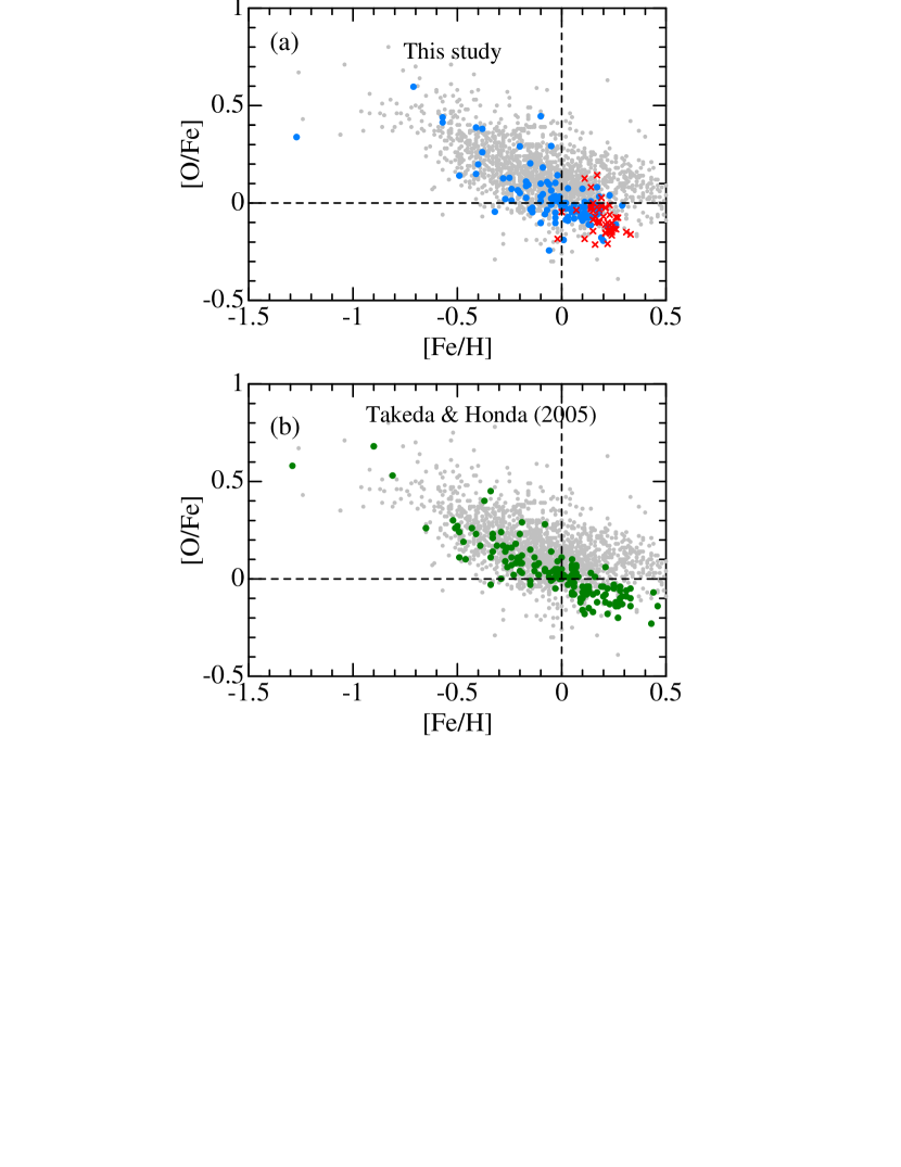
Figure 13: (a) The [O/Fe] ratios derived in this study for each of the program stars (47 Hyades stars and 101 field stars) are plotted against [Fe/H], where the meanings of the symbols are the same as in Figure 1. (b) Takeda & Honda’s (2005) [O/Fe] vs. [Fe/H] relation derived for the 160 mid-F through early K stars based on the O i 7771–5 lines. In both panels (a) and (b) are also plotted the similar correlations taken from Hawkins et al. (2016) by gray dots for comparison, which were derived from the high-resolution infrared spectra for a large APOGEE+Kepler stellar sample (APOKASC).

Turning our attention to field stars, we compare our oxygen abundances with those derived by three previous studies (as done in Section 5.1 for stellar parameters). The panels (e) and (f) of Figures 8, 9, and 10 show comparison of our (non-LTE) [O/H] and [O/Fe] values with those of Wang et al. (2009: from O i 7771–5 with non-LTE), Ramírez et al. (2013; from O i 7771-5 with non-LTE), and Luck (2017; from [O i] 6300 with LTE), respectively. These figures suggest that rough correlation is observed (though not necessarily good) between our and their results. In addition, in Figure 13 is compared the non-LTE [O/Fe] vs. [Fe/H] relation derived in this study for 148 G–K dwarfs (47 Hyades stars at 6300 K $\gtrsim T_{\rm eff}\gtrsim$ 4500 K and 101 field stars at 5500 K $\gtrsim T_{\rm eff}\gtrsim$ 4500 K) with the similar relation obtained by Takeda & Honda (2005) based on the same O i 7771–5 triplet (with non-LTE) for early F–early K dwarfs/subgiants (at 7000 K $\gtrsim T_{\rm eff}\gtrsim$ 5000 K). It can be confirmed by comparing panels (a) and (b) of Figure 13 that quite a similar trend of [O/Fe] (i.e., increasing with a decrease in [Fe/H] with almost the same gradient) is observed for both cases. This is a reasonable consequence, because most of the sample stars belong to the thin-disk population in this study (cf. Section 3.2) as well as in Takeda & Honda (2005) (cf. Sect. 2.2 in Takeda 2007). For comparison, the similar relations between [O/Fe] and [Fe/H] derived by Hawkins et al. (2016) for a large number of disk stars (APOGEE+Kepler sample) are overplotted in these figures. Although the global tendency of decreasing [O/Fe] with an increase in [Fe/H] is similar, their [O/Fe] tends to be stagnant and supersolar (i.e., $\gtrsim 0$) at [Fe/H] $\gtrsim 0$ unlike our results ([O/Fe] $\lesssim 0$ at at [Fe/H] $\gtrsim 0$). See also Sect. 4.1 in Hawkins et al. (2016).

Combining all the results mentioned above, we may conclude that oxygen abundances can be reliably determined based on the O i triplet lines at 7771–5 Å for K dwarfs (just like F and G stars), as long as stars of $T_{\rm eff}\gtrsim 4500$ K are concerned (actually, $\sim 4500$ K corresponding to spectral type of $\sim$ K 5 is the practical lower limit of $T_{\rm eff}$, below which these high-excitation O i lines become too weak to be usable).

6 SUMMARY AND CONCLUSION

It has been reported that Fe abundances of K dwarfs derived from Fe i and Fe ii lines tend to show considerable discrepancy (i.e., the latter is larger than the former), becoming progressively more serious with a decrease in $T_{\rm eff}$. If it is real, the widely used spectroscopic method for determining the parameters of solar-type stars based on Fe lines (which makes use of ionization equilibrium of Fe i/Fe ii) would hardly be applicable to K dwarfs, since classical model atmospheres would be no more valid for them.

According to the recent investigations of Aleo et al. (2017) and Tsantaki ey al. (2019), however, the alleged large Fe ii–Fe i disagreement in K dwarfs is likely to be due to the use of blending-affected Fe ii lines, and can be appreciably mitigated down to a practically insignificant level when they are removed. This may suggest the necessity of reexamining another similar problem related to K dwarfs (argued by Schuler et al. from their studies on open cluster stars) that oxygen abundances derived from the high-excitation O i 7771–5 triplet lines are strikingly overestimated (even by up to $\sim 1$ dex), its extent becoming more prominent towards lower $T_{\rm eff}$.

Motivated by this situation, we decided to reexamine whether these “spectroscopic K dwarf problems” really exist, based on the spectral data of 148 G–K dwarfs (47 Hyades stars and 101 field stars). This may be checked by applying the conventional method of analysis (for determining stellar parameters and oxygen abundances) to these program stars. That is, some kind of unreasonable or inconsistent result must be observed if the classical modeling really breaks down for K dwarfs.

We determined $T_{\rm eff}$, $\log g$, $v_{\rm t}$, and [Fe/H] for all the program stars based on the equivalent widths of Fe i and Fe ii lines as done by Takeda et al. (2005). Comparing our spectroscopic $T_{\rm eff}$ and $\log g$ of Hyades stars with those of de Bruijne et al. (2001) (which are considered to be well established), we found that the differences are practically not so significant (especially, no evidence was found that K dwarfs suffer larger errors than G dwarfs). This result may support Aleo et al.’s (2017) conclusion that the differences between Fe i and Fe ii abundances in K dwarfs are actually not so important ($\lesssim 0.1$ dex) at least for stars of $T_{\rm eff}\gtrsim 4500$ K.

The oxygen abundances of these G–K dwarfs were derived by applying the spectrum-fitting technique to the 7770–7782 Å region comprising O i 7771–5 and Fe i 7780 lines, where the non-LTE effect was taking into account for the O i lines. Regarding the [O/H] values of Hyades stars, our results turned out to distribute around $\sim+0.2$ (being consistent with the expectation that cluster stars should have similar abundances), in marked contrast with the progressively increasing tendency (even up to $\sim+1$) towards lower $T_{\rm eff}$ reported by Schuler et al. (2006a).

We investigated the reason for this distinct discrepancy, and found that the higher $T_{\rm eff}$ scale adopted by them is the main cause, which has a large impact on the abundances derived from O i lines of high-excitation. It was also confirmed that the [O/Fe] vs. [Fe/H] relation we obtained for 101 field mid G–mid K stars is quite similar to that derived by Takeda & Honda (2005) for 160 stars (mainly F–G type), which means that K dwarfs can not be exceptionally anomalous in terms of oxygen abundance determination based on the O i 7771–5 triplet.

In summary, we conclude for K dwarfs that their atmospheric parameters can be spectroscopically evaluated to a sufficient precision in the conventional manner using Fe lines (because the classical Saha–Boltzmann equation for Fe i/Fe ii is still not a bad assumption) and oxygen abundances can be reliably established from the high-excitation O i 7771–5 triplet (just like F–G dwarfs), so far as stars of $T_{\rm eff}\gtrsim 4500$ K are concerned.

This investigation is based in part on the data collected at Subaru Telescope, which is operated by the National Astronomical Observatory of Japan. Data reduction was in part carried out by using the common-use data analysis computer system at the Astronomy Data Center (ADC) of the National Astronomical Observatory of Japan. This research has made use of the SIMBAD database, operated by CDS, Strasbourg, France. This work also used the data from the European Space Agency (ESA) mission Gaia, processed by the Gaia Data Processing and Analysis Consortium (DPAC). Funding for the DPAC has been provided by national institutions, in particular the institutions participating in the Gaia Multilateral Agreement.

Appendix A IMPACT OF EFFECTIVE TEMPERATURE SCALE ON [O/H] IN PREVIOUS STUDIES OF OPEN CLUSTERS

We showed in Section 5.2 that the conspicuous excess of [O/H] increasing toward a lower $T_{\rm eff}$ concluded by Schuler et al. (2006a) for Hyades stars could be interpreted as mainly due to the systematically lower $T_{\rm eff}$ scale they adopted (cf. Figure 12). Regarding the similar tendencies in [O/H] (based on the high-excitation O i 7771–5 triplet lines) also reported by several authors for open clusters other than Hyades (i.e., UMa moving group, M 34, Pleiades, NGC 752; cf. Section 1), we are unable to check them directly as done in Figure 12. Still, however, we can examine whether the $T_{\rm eff}$ scales adopted by those previous studies are reasonable and how they affect the [O/H] trends.

We first postulate that Casagrande et al.’s (2010) calibration yields reasonably correct $T_{\rm eff}$, which we confirmed to be consistent with our spectroscopic $T_{\rm eff}$ (cf. Figures 11a and 11b). Since $T_{\rm eff}$ values were derived photometrically from $B-V$ colors by using any of the following three formulas in most of these relevant studies (cf. Table 2 for a brief summary), the effect we want to examine is essentially attributed to the difference of these equations from that of Casagrande et al. (2010).

$$\begin{split}T_{\rm eff}&=5040/\bigl{(}0.5247+0.5396(B-V)_{0}\bigr{)}\\ &+701.7(B-V)_{0}\bigl{(}[{\rm Fe/H}]-[{\rm Fe/H}]_{\rm Hyades}\bigr{)},\end{split}$$ (A1)

$$T_{\rm eff}=1808(B-V)_{0}^{2}-6103(B-V)_{0}+8899,$$ (A2)

and

$$\begin{split}T_{\rm eff}&=8344-3631.32(B-V)_{0}-2211.81(B-V)_{0}^{2}\\ &+3365.44(B-V)_{0}^{3}-1033.62(B-V)_{0}^{4}\\ &+701.7\bigl{(}[{\rm Fe/H}]-[{\rm Fe/H}]_{\rm Hyades}\bigr{)},\end{split}$$ (A3)

where $T_{\rm eff}$ is in K, $(B-V)_{0}$ is the reddening-corrected $B-V$ color, [Fe/H] is the metallicity of a star, and [Fe/H]_Hyades is the Hyades metallicity (assumed to be 0.15 in this study). These $T_{\rm eff}$ vs. $(B-V)_{0}$ relations of Equations (A1), (A2), and (A3) are compared with that of Casagrande et al. (2010) in Figure 14a, where we can see that all the former three tend to yield systematically lower $T_{\rm eff}$ than the latter at $(B-V)_{0}\gtrsim 0.6$ with discrepancies increasing towards lower $T_{\rm eff}$.

For each star, $T_{\rm eff}^{\rm Casagrande}$ was computed from $(B-V)_{0}$ (taken from the relevant paper) and assumed cluster [Fe/H] (cf. Table 2) according to Casagrande et al.’s (2010) recipe and compared with literature value ($T_{\rm eff}^{\rm literature}$) actually adopted therein. The differences $\chi_{\rm low}\theta_{\rm eff}^{\rm literature}-\chi_{\rm low}\theta_{\rm eff}^{\rm Casagrande}$ (see the caption of Figure 12e for the meanings of $\theta_{\rm eff}$ and $\chi_{\rm low}$) are plotted against $T_{\rm eff}^{\rm Casagrande}$ in Figure 14b, from which we can read the following characteristics.

• In all cases, the differences between $\chi_{\rm low}\theta_{\rm eff}^{\rm literature}$ and $\chi_{\rm low}\theta_{\rm eff}^{\rm Casagrande}$, which correspond to the expected overestimation of [O/H] due to an underestimated $T_{\rm eff}$ (cf. Section 5.2), tend to progressively increase with a lowering of $T_{\rm eff}$; i.e., from $\sim 0.0$ dex (at $\sim 6000$ K) to $\sim$ 0.3–0.5 dex (at $\sim 5000$ K). This reasonably explains the $T_{\rm eff}$-dependent tendency of [O/H] concluded in their papers (cf. Table 2) at least qualitatively, which indicates that the inappropriate $T_{\rm eff}$ scale is the main cause for the trend.

• Quantitatively, however, only this $T_{\rm eff}$-related correction seems to be rather insufficient to account for the differences ([O/H]${}_{5000}-$[O/H]₆₀₀₀) ranging from $\sim$ 0.2 dex to $\sim$ 0.7 dex (Table 2), which means that some other factors (such as an underestimation of $W_{\lambda}$ for the very weak line case at the low-$T_{\rm eff}$ regime; cf. Figure 12f) may also be involved.

• Especially, as seen from Fig. 2 of Schuler et al. (2004), the d[O/H]/d$T_{\rm eff}$ gradient of Pleiades and M 34 cluster stars at $T_{\rm eff}\lesssim$ 5200 K appears to become abruptly steeper. Since these two open clusters are younger than the Hyades and thus stellar activity should be higher, a possibility may not be excluded that some activity-related effect might influence the strength of high-excitation O i triplet for these cases. Accordingly, oxygen abundances from O i 7771–5 lines for dwarfs of these younger clusters at the $T_{\rm eff}$ regime of 4500 K $\lesssim T_{\rm eff}\lesssim 5500$ K may be worth careful reinvestigation based on reliable $T_{\rm eff}$ scales.

Table 1: Basic data, parameters, and abundance results of 148 program stars.

HIP	HD	$V$	$M_{V}$	$B-V$	$T_{\rm eff}$	$\log g$	$v_{\rm t}$	[Fe/H]	$v_{\rm M}$	[O/H]	$\Delta_{7774}$	$W_{7774}$
(1)	(2)	(3)	(4)	(5)	(6)	(7)	(8)	(9)	(10)	(11)	(12)	(13)
(Hyades stars)
19796	26784	7.11	3.73	0.51	6307	4.29	1.37	0.26	13.74	0.19	$-$0.23	125.4
22566	30809	7.90	4.07	0.53	6250	4.29	1.10	0.24	9.06	0.14	$-$0.21	113.1
19386	26257	7.64	3.57	0.55	6201	4.26	1.03	0.23	6.31	0.12	$-$0.21	108.2
20557	27808	7.13	4.07	0.52	6199	4.27	1.21	0.19	10.45	0.17	$-$0.21	114.9
20815	28205	7.41	4.11	0.54	6180	4.35	1.07	0.19	8.67	0.22	$-$0.20	113.2
25639	35768	8.50	3.82	0.56	6138	4.08	1.13	0.15	5.83	0.06	$-$0.23	105.8
20237	27406	7.46	4.20	0.56	6134	4.37	1.07	0.27	9.59	0.19	$-$0.18	106.8
15304	20430	7.38	3.91	0.57	6125	4.29	0.99	0.33	5.97	0.17	$-$0.18	104.5
10672	14127	8.55	4.48	0.57	6125	4.41	0.88	0.01	6.58	$-$0.05	$-$0.16	84.2
22422	30589	7.72	4.19	0.58	6081	4.39	0.97	0.24	5.54	0.07	$-$0.15	90.9
19148	25825	7.85	4.50	0.59	6078	4.47	1.05	0.21	6.14	0.06	$-$0.14	87.8
15310	20439	7.78	4.46	0.62	6003	4.48	1.01	0.31	5.99	0.16	$-$0.14	89.3
20577	27859	7.79	4.37	0.60	5955	4.30	0.96	0.14	6.44	0.11	$-$0.16	87.5
21317	28992	7.90	4.73	0.63	5928	4.48	0.98	0.20	5.55	0.13	$-$0.12	81.5
19786	26767	8.05	4.78	0.64	5922	4.42	1.07	0.23	5.60	0.08	$-$0.12	79.4
20899	28344	7.83	4.45	0.61	5902	4.30	1.11	0.15	6.68	0.15	$-$0.15	86.9
20741	28099	8.10	4.75	0.66	5852	4.55	0.92	0.24	4.42	0.12	$-$0.10	72.6
19793	26736	8.05	4.73	0.66	5815	4.38	0.99	0.22	5.78	0.12	$-$0.12	74.6
19781	26756	8.45	5.15	0.69	5745	4.54	0.91	0.22	5.13	0.08	$-$0.09	62.7
20146	27282	8.47	5.11	0.72	5677	4.48	0.93	0.24	5.32	0.09	$-$0.09	60.0
23750	240648	8.82	5.19	0.73	5630	4.57	0.89	0.25	5.38	0.12	$-$0.07	56.5
14976	19902	8.15	5.03	0.73	5614	4.57	0.91	0.18	3.72	0.08	$-$0.07	53.7
20130	27250	8.62	5.48	0.74	5591	4.55	1.00	0.18	4.59	0.08	$-$0.07	52.6
23069	31609	8.89	5.36	0.74	5583	4.53	0.84	0.21	3.87	0.10	$-$0.07	53.1
24923	242780	9.03	5.34	0.77	5560	4.57	0.85	0.27	5.04	0.12	$-$0.07	52.0
21099	28593	8.59	5.28	0.73	5557	4.44	0.99	0.17	4.68	0.07	$-$0.08	52.2
23498	32347	9.00	5.33	0.77	5549	4.52	1.03	0.21	4.96	0.05	$-$0.07	49.2
20949	283704	9.19	5.35	0.77	5544	4.57	0.88	0.23	3.75	0.09	$-$0.07	49.3
20480	27732	8.84	5.41	0.76	5539	4.49	1.00	0.15	4.55	0.11	$-$0.07	52.2
21741	284574	9.40	5.42	0.81	5425	4.55	0.95	0.23	5.00	0.17	$-$0.06	46.2
19934	284253	9.14	5.59	0.81	5376	4.57	0.87	0.17	3.71	0.15	$-$0.05	41.9
20951	285773	8.95	5.87	0.83	5350	4.57	1.02	0.14	3.90	0.12	$-$0.05	39.6
22380	30505	8.98	5.63	0.83	5336	4.57	0.94	0.21	4.49	0.19	$-$0.05	41.1
20850	28258	9.02	5.66	0.84	5321	4.50	1.04	0.18	4.19	0.15	$-$0.05	39.9
20492	27771	9.11	5.74	0.85	5292	4.60	0.89	0.22	4.38	0.01	$-$0.04	31.2
20978	28462	9.08	6.04	0.86	5242	4.50	1.04	0.16	4.74	0.09	$-$0.04	33.3
18327	285252	8.99	5.91	0.90	5183	4.61	1.02	0.21	4.27	0.18	$-$0.04	31.9
19098	285367	9.31	5.79	0.89	5123	4.56	1.03	0.11	4.41	0.24	$-$0.04	31.6
23312	$\cdots$	9.71	5.83	0.96	5104	4.53	0.90	0.14	4.00	0.22	$-$0.04	30.1
20827	285830	9.48	5.67	0.93	5089	4.61	0.89	0.23	3.88	0.22	$-$0.03	28.2
20082	285690	9.57	6.08	0.98	5030	4.53	0.79	0.15	3.60	0.01	$-$0.03	21.7
19263	285482	9.94	6.41	1.00	4898	4.50	0.85	0.07	4.24	0.03	$-$0.02	17.0
22654	284930	10.29	6.68	1.07	4831	4.47	0.99	0.11	4.22	$-$0.07	$-$0.02	12.5
18946	$\cdots$	10.12	6.94	1.09	4823	4.64	0.92	0.16	3.46	$-$0.05	$-$0.01	11.5
20762	286789	10.48	7.18	1.15	4729	4.25	1.15	$-$0.02	4.51	$-$0.20	$-$0.02	9.0
18322	286363	10.12	7.24	1.07	4725	4.71	0.91	0.17	3.97	0.31	$-$0.01	14.2
19441	$\cdots$	10.10	7.47	1.19	4525	4.61	0.70	0.14	3.56	0.11	$-$0.01	6.3
(Field stars)
053471	94718	8.45	5.58	0.73	5482	4.45	0.73	$-$0.03	3.47	$-$0.13	$-$0.06	37.2
082588	152391	6.65	5.51	0.75	5475	4.50	0.94	0.02	4.15	$-$0.01	$-$0.06	42.0
004907	5996	7.67	5.61	0.76	5445	4.53	0.96	$-$0.09	3.68	$-$0.05	$-$0.06	38.6
010818	14374	8.48	5.51	0.74	5444	4.58	0.80	$-$0.01	3.42	$-$0.02	$-$0.05	38.4
026653	37216	7.85	5.63	0.76	5441	4.58	0.94	$-$0.03	3.48	$-$0.02	$-$0.05	38.5
059280	105631	7.46	5.53	0.79	5439	4.50	0.88	0.19	3.57	0.01	$-$0.06	40.5
040419	69076	8.27	5.61	0.71	5434	4.47	0.66	$-$0.24	3.47	$-$0.23	$-$0.05	31.3
093926	178450	7.78	5.54	0.76	5423	4.45	2.00	$-$0.04	18.51	0.24	$-$0.07	57.4

Table 1: (Continued.)

HIP	HD	$V$	$M_{V}$	$B-V$	$T_{\rm eff}$	$\log g$	$v_{\rm t}$	[Fe/H]	$v_{\rm M}$	[O/H]	$\Delta_{7774}$	$W_{7774}$
(1)	(2)	(3)	(4)	(5)	(6)	(7)	(8)	(9)	(10)	(11)	(12)	(13)
043852	76218	7.69	5.60	0.77	5422	4.59	0.83	0.03	4.34	$-$0.04	$-$0.05	35.9
094346	180161	7.04	5.53	0.80	5418	4.49	0.95	0.17	3.67	0.11	$-$0.06	44.2
055210	98281	7.29	5.58	0.73	5401	4.47	0.75	$-$0.21	3.24	$-$0.15	$-$0.05	33.1
112245	215500	7.50	5.50	0.72	5399	4.39	0.62	$-$0.20	3.15	$-$0.15	$-$0.06	33.8
046843	82443	7.05	5.80	0.78	5393	4.65	1.27	$-$0.03	5.38	0.07	$-$0.05	39.5
098677	190067	7.15	5.72	0.71	5376	4.48	0.64	$-$0.32	3.23	$-$0.37	$-$0.04	24.4
065515	116956	7.29	5.59	0.80	5372	4.51	1.07	0.14	5.30	0.11	$-$0.05	41.5
115331	220182	7.36	5.66	0.80	5368	4.56	1.08	0.06	4.98	0.01	$-$0.05	36.3
007576	10008	7.66	5.79	0.80	5358	4.52	0.97	$-$0.03	3.48	$-$0.11	$-$0.04	31.6
062016	110514	8.04	5.61	0.80	5358	4.49	0.73	$-$0.01	3.40	$-$0.01	$-$0.05	35.4
075277	136923	7.16	5.64	0.80	5357	4.56	0.67	$-$0.05	3.35	$-$0.06	$-$0.04	32.4
010798	14412	6.33	5.81	0.72	5357	4.51	0.73	$-$0.49	3.30	$-$0.35	$-$0.04	24.9
010276	13483	8.46	5.81	0.78	5347	4.54	0.85	$-$0.17	3.41	$-$0.08	$-$0.05	31.9
042074	72760	7.32	5.63	0.79	5344	4.59	0.92	0.09	3.64	0.07	$-$0.04	36.4
050782	89813	7.78	5.64	0.75	5336	4.51	0.67	$-$0.07	3.28	$-$0.11	$-$0.04	30.3
081813	151541	7.56	5.63	0.77	5334	4.42	0.66	$-$0.14	3.40	$-$0.17	$-$0.05	29.6
028954	41593	6.76	5.81	0.81	5332	4.50	1.04	0.05	4.54	0.00	$-$0.05	34.7
106122	204814	7.93	5.56	0.76	5327	4.44	0.66	$-$0.20	3.18	0.09	$-$0.06	39.4
000400	225261	7.82	5.78	0.76	5323	4.49	0.62	$-$0.38	3.25	$-$0.12	$-$0.05	30.3
077408	141272	7.44	5.79	0.80	5304	4.45	1.01	0.02	4.20	$-$0.07	$-$0.05	31.3
051819	90343	7.29	5.68	0.82	5303	4.50	0.78	0.12	3.50	0.04	$-$0.05	34.2
014023	18702	8.11	5.56	0.84	5280	4.47	0.74	0.18	3.09	0.21	$-$0.05	40.0
085235	158633	6.44	5.90	0.76	5270	4.54	0.60	$-$0.41	3.05	$-$0.26	$-$0.04	24.5
074702	135599	6.92	5.96	0.83	5250	4.63	0.90	$-$0.04	4.05	$-$0.01	$-$0.04	28.6
116085	221354	6.76	5.63	0.84	5246	4.53	0.64	0.10	3.01	0.17	$-$0.04	35.6
072200	130215	7.98	5.87	0.87	5244	4.56	0.88	0.13	3.42	0.05	$-$0.04	31.0
039157	65583	6.97	5.84	0.72	5243	4.54	0.53	$-$0.71	3.00	$-$0.11	$-$0.05	27.3
082267	151877	8.40	5.85	0.82	5237	4.59	0.69	$-$0.10	3.04	$-$0.09	$-$0.04	25.9
002742	3141	8.02	5.71	0.87	5225	4.51	0.69	0.18	3.04	0.13	$-$0.04	32.9
012926	17190	7.89	5.84	0.84	5224	4.61	0.61	$-$0.05	3.10	$-$0.03	$-$0.04	26.8
033848	52456	8.16	5.90	0.86	5212	4.51	0.69	0.06	3.25	$-$0.02	$-$0.04	27.6
078241	143291	8.02	5.94	0.76	5208	4.40	0.50	$-$0.40	3.22	$-$0.20	$-$0.04	24.0
039064	65430	7.68	5.86	0.83	5202	4.55	0.57	$-$0.09	2.99	0.09	$-$0.04	30.5
008543	11130	8.06	5.92	0.76	5197	4.52	0.52	$-$0.57	2.92	$-$0.13	$-$0.04	24.7
000184	224983	8.48	5.85	0.89	5195	4.55	0.73	0.13	2.94	0.02	$-$0.04	27.5
061099	108984	7.91	5.90	0.86	5194	4.54	0.60	0.11	3.14	0.09	$-$0.04	29.6
010532	13977	9.11	5.79	0.88	5188	4.58	0.72	0.11	3.20	0.06	$-$0.04	28.2
066781	119332	7.77	5.89	0.83	5187	4.46	0.68	$-$0.03	3.21	0.00	$-$0.04	27.9
054906	97658	7.76	6.12	0.84	5175	4.58	0.61	$-$0.27	3.05	$-$0.25	$-$0.03	20.4
006379	7924	7.17	6.04	0.83	5173	4.60	0.65	$-$0.15	2.99	$-$0.07	$-$0.03	25.8
007830	10261	8.92	5.84	0.91	5165	4.59	0.88	0.04	3.50	0.01	$-$0.03	27.1
015099	20165	7.83	6.09	0.86	5164	4.56	0.65	0.01	3.11	0.01	$-$0.03	25.9
073005	132142	7.77	5.88	0.79	5157	4.53	0.38	$-$0.38	2.98	0.00	$-$0.04	26.6
013891	18450	8.21	5.93	0.87	5154	4.55	0.56	$-$0.06	3.02	0.03	$-$0.04	26.4
006613	8553	8.49	5.89	0.91	5129	4.61	0.59	0.00	2.99	$-$0.02	$-$0.03	24.7
112527	216520	7.53	6.03	0.87	5123	4.52	0.57	$-$0.14	3.12	$-$0.19	$-$0.03	20.8
064457	114783	7.56	6.01	0.93	5121	4.47	0.69	0.13	3.03	0.06	$-$0.04	26.5
036704	59747	7.68	6.21	0.86	5120	4.60	0.85	0.03	3.36	0.10	$-$0.03	28.0
114886	219538	8.07	6.15	0.87	5110	4.56	0.65	0.01	2.98	$-$0.02	$-$0.03	24.4
090790	170657	6.81	6.21	0.86	5087	4.38	0.64	$-$0.17	3.45	$-$0.14	$-$0.04	22.2
012158	16287	8.10	6.17	0.94	5081	4.54	1.00	0.14	3.91	0.03	$-$0.03	24.0
072312	130307	7.76	6.29	0.89	5078	4.55	0.75	$-$0.15	3.44	$-$0.18	$-$0.03	18.6
098505	189733	7.67	6.25	0.93	5076	4.42	1.06	0.03	4.14	$-$0.06	$-$0.03	22.5
053486	94765	7.37	6.15	0.92	5076	4.59	0.94	0.06	3.82	0.05	$-$0.03	24.0
013976	18632	7.97	6.12	0.93	5075	4.59	0.98	0.19	3.85	0.17	$-$0.03	27.5

Table 1: (Continued.)

HIP	HD	$V$	$M_{V}$	$B-V$	$T_{\rm eff}$	$\log g$	$v_{\rm t}$	[Fe/H]	$v_{\rm M}$	[O/H]	$\Delta_{7774}$	$W_{7774}$
(1)	(2)	(3)	(4)	(5)	(6)	(7)	(8)	(9)	(10)	(11)	(12)	(13)
098828	190470	7.82	6.15	0.92	5071	4.62	0.77	0.17	3.04	0.14	$-$0.03	26.6
026505	37008	7.74	6.18	0.83	5054	4.58	0.09	$-$0.41	2.79	$-$0.02	0.01	22.8
108156	208313	7.73	6.19	0.91	5051	4.59	0.72	$-$0.01	3.04	0.02	$-$0.03	22.5
108028	208038	8.18	6.28	0.94	5035	4.62	0.84	$-$0.05	3.57	0.01	$-$0.03	21.2
011083	14687	8.83	6.18	0.91	5033	4.58	0.59	0.08	2.94	0.04	$-$0.03	22.4
057939	103095	6.42	6.61	0.75	5033	4.38	$-$0.10	$-$1.27	3.28	$-$0.93	$-$0.03	5.1
017420	23356	7.10	6.36	0.93	5030	4.57	0.80	$-$0.08	3.11	$-$0.14	$-$0.03	17.6
088972	166620	6.38	6.15	0.88	5019	4.62	0.28	$-$0.15	2.73	0.05	$-$0.03	22.4
098792	190404	7.28	6.32	0.81	5016	4.65	$-$0.18	$-$0.57	2.93	$-$0.16	$-$0.03	16.6
003206	3765	7.36	6.17	0.94	5000	4.53	0.77	0.14	3.02	0.15	$-$0.03	24.4
092919	175742	8.16	6.50	0.91	4983	4.48	2.13	$-$0.10	11.88	0.34	$-$0.04	31.6
049699	87883	7.56	6.28	0.96	4980	4.62	0.56	0.11	2.79	0.11	$-$0.03	21.7
071395	128311	7.48	6.38	0.97	4967	4.67	0.88	0.16	4.03	0.15	$-$0.02	20.9
003535	4256	8.03	6.32	0.98	4954	4.47	0.75	0.26	3.06	0.15	$-$0.03	22.7
084195	155712	7.95	6.39	0.94	4947	4.43	0.57	$-$0.10	3.16	$-$0.07	$-$0.03	17.9
072146	130004	7.87	6.42	0.93	4930	4.57	0.49	$-$0.24	2.97	$-$0.17	$-$0.02	13.9
033852	51866	7.98	6.43	0.99	4927	4.56	0.69	0.10	3.15	0.01	$-$0.02	17.2
084616	156985	7.93	6.59	1.02	4916	4.39	0.61	$-$0.06	3.31	$-$0.30	$-$0.02	12.0
035872	57901	8.19	6.20	0.96	4908	4.58	0.53	0.17	2.91	0.25	$-$0.03	22.4
068184	122064	6.49	6.47	1.04	4908	4.49	0.67	0.23	3.13	0.09	$-$0.02	19.0
066147	117936	7.98	6.65	1.03	4872	4.28	0.95	0.01	3.63	$-$0.18	$-$0.02	13.3
071181	128165	7.24	6.60	1.00	4868	4.60	0.78	$-$0.03	2.97	$-$0.08	$-$0.02	12.8
046580	82106	7.20	6.68	1.00	4861	4.59	0.88	$-$0.02	3.55	0.12	$-$0.02	16.7
000974	$\cdots$	8.73	6.68	1.04	4852	4.67	0.57	0.02	3.00	0.02	$-$0.02	13.8
023311	32147	6.22	6.49	1.05	4815	4.49	0.66	0.29	2.95	0.28	$-$0.02	19.4
069526	124642	8.03	6.84	1.06	4798	4.51	0.90	0.10	4.00	0.03	$-$0.02	13.2
010416	13789	8.55	6.75	1.05	4782	4.64	0.86	0.09	3.31	0.02	$-$0.01	11.6
105038	202575	7.88	6.84	1.02	4777	4.66	0.75	$-$0.07	3.57	0.04	$-$0.01	11.9
032010	47752	8.08	6.86	1.02	4776	4.53	0.78	$-$0.17	3.16	$-$0.06	$-$0.02	11.2
025220	35171	7.93	7.15	1.10	4757	4.43	1.06	$-$0.10	4.04	$-$0.20	$-$0.02	8.9
008275	10853	8.91	7.10	1.04	4739	4.73	0.66	$-$0.10	3.29	0.00	$-$0.01	9.8
011000	14635	9.07	6.93	1.08	4732	4.71	0.70	0.19	3.40	0.17	$-$0.01	12.1
015919	21197	7.86	6.96	1.15	4717	4.22	0.89	0.14	3.34	0.07	$-$0.02	13.3
005286	6660	8.41	6.83	1.12	4716	4.45	0.72	0.20	3.25	0.01	$-$0.01	10.7
098698	190007	7.46	6.87	1.13	4677	4.50	0.79	0.22	3.34	0.10	$-$0.01	10.5
013258	17660	8.87	7.12	1.19	4643	4.32	0.67	0.23	3.25	0.27	$-$0.02	13.5
104214	201091	5.21	7.49	1.18	4523	4.57	0.32	$-$0.28	3.18	$-$0.15	$-$0.01	4.4
$\cdots$	131156B	6.82	7.67	1.17	4495	4.55	0.67	$-$0.25	3.59	$-$0.12	$-$0.01	4.2

(1) Hipparcos Catalog number. (2) Henry-Draper Catalog number. (3) Apparent visual magnitude (in mag). (4) Absolute visual magnitude (in mag). (5) $B-V$ color (in mag). (6) Effective temperature (in K). (7) Logarithmic surface gravity (cm s^-2/dex). (8) Microturbulent velocity dispersion (in km s^-1). (9) Fe abundance relative to the Sun (in dex). (10) Macrobroadening velocity (in km s^-1). (11) Non-LTE oxygen abundance relative to the Sun, $A^{\rm NLTE}$(O)$-8.861$ (in dex), where 8.861 is the solar non-LTE oxygen abundance derived in the same manner (cf. Takeda et al. 2015). (12) Non-LTE correction ($\equiv A^{\rm N}-A^{\rm L}$) (in dex) for O I 7774.166 (middle line of the triplet). (13) Equivalent width for O I 7774.166 (in mÅ).
In each of the stellar group (47 Hyades stars and 101 field stars), the data are arranged in the decreasing order of $T_{\rm eff}$ similarly to Figures 4 and 5, so that a direct comparison may be possible. (See “tableE1.dat” of the online material for the data arranged in the increasing order of HIP number for each group.)

Table 2: Published [O/H] derivations from O i 7771–5 lines for open cluster stars.

Cluster	Ref.	Figure	[O/H]5000	[O/H]6000	$T_{\rm eff}$ formula	[Fe/H]	Remark
(1)	(2)	(3)	(4)	(5)	(6)	(7)	(8)
Hyades	SCH06	Fig. 3	$\sim 0.5$	$\sim 0.2$	Equation (A1)	+0.15
Pleiades	SCH04	Fig. 1	$\sim 0.9$	$\sim 0.2$	Equation (A2)	+0.01	See also Fig. 4 in KS05.
M 34	SCH04	Fig. 1	$\sim 0.8$	$\sim 0.1$	$\cdots$	+0.07	Spectroscopic $T_{\rm eff}$.
UMa group	KS05	Fig. 4	$\sim 0.3$	$\sim 0.1$	Equation (A3)	$-0.08$
Hyades	MAD13	Fig. 4	$\cdots$	$\sim 0.2$	Equation (A1)	+0.15	Lowest $T_{\rm eff}$ $\sim 5400$ K, where [O/H] $\sim 0.3$.
NGC 752	MAD13	Fig. 5	$\sim 0.7$	$\sim-0.1$	Equation (A1)	$-0.06$	E($B-V$) = 0.035 was adopted.

(1) Cluster name. (2) Reference key: SCH06 — Schuler et al. (2006a), SCH04 — Schuler et al. (2004), KS05 — King & Schuler (2005), MAD13 — Maderak et al. (2013). (3) Figure number of the relevant paper where [O/H] vs. $T_{\rm eff}$ plots for cluster stars are presented. (4) Rough value of [O/H] at $T_{\rm eff}\sim 5000$ K. (5) Rough value of [O/H] at $T_{\rm eff}\sim 6000$ K. (6) $T_{\rm eff}$ vs. $(B-V)_{0}$ formula adopted in the relevant study for evaluation of $T_{\rm eff}$. (7) [Fe/H] of the cluster, which we used for evaluation of $T_{\rm eff}^{\rm Casagrande}$ (cf. Figure 14b) by using Casagrande et al.’s (2010) relation. (8) Specific remark.

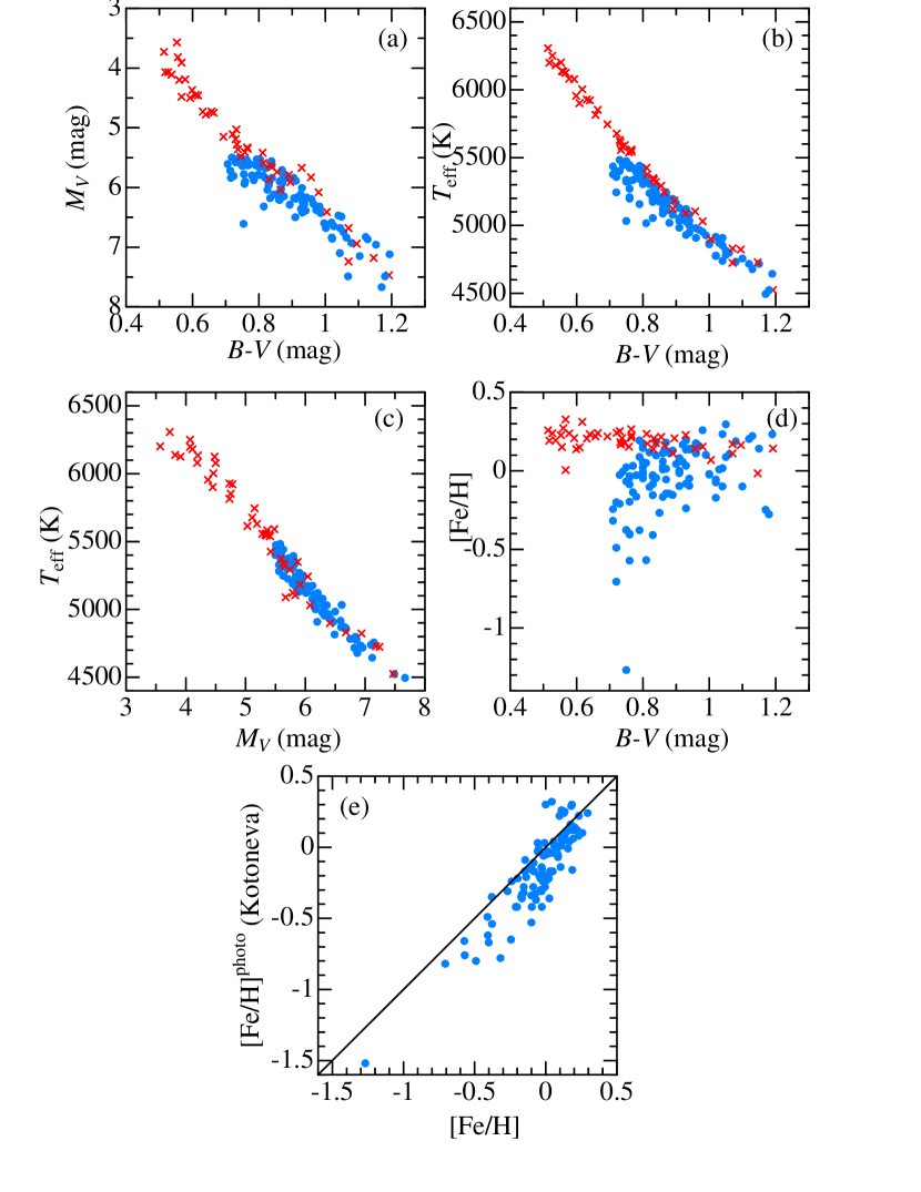
Figure 1: Panels (a)–(d) are the correlation diagram between the photometric data (absolute visual magnitude $M_{V}$ and $B-V$ color, mainly derived from the Hipparcos catalog) and the spectroscopically determined atmospheric parameters (cf. Section 3.1) of the program stars: (a) $M_{V}$ vs. $B-V$, (b) $T_{\rm eff}$ vs. $B-V$, (c) $T_{\rm eff}$ vs. $M_{V}$. and (d) [Fe/H] vs. $B-V$. Panel (e) shows the interrelationship between the spectroscopic metallicity established in this study (abscissa) and the photometric metallicity ([Fe/H]^photo) evaluated by Kotoneva et al. (2002) based on the position in the color–magnitude diagram (ordinate). Our program stars of 47 Hyades stars and 101 field stars are separately represented by red crosses and blue circles, respectively.

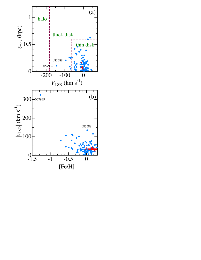
Figure 3: (a) Correlation diagram between the maximum separation from the galactic plane ($z_{\rm max}$) and the rotation velocity component relative to the Local Standard of Rest ($V_{\rm LSR}$), which may be used for classifying the stellar population (the boundaries are indicated by the dashed lines; cf. Ibukiyama & Arimoto 2002). (b) Space velocity relative to the Local Standard of Rest [$|v_{\rm LSR}|\equiv(U_{\rm LSR}^{2}+V_{\rm LSR}^{2}+W_{\rm LSR}^{2})^{1/2}$] plotted against [Fe/H]. Same meanings of the symbols as in Figure 1.

Figure 4: Synthetic spectrum fitting in the 7770–7782 Å region comprising the O i 7771–5 and Fe i 7780 lines for 47 Hyades stars. The best-fit theoretical spectra are shown by dark blue solid lines. The observed data used in the fitting are plotted by red symbols, while those rejected in the fitting (e.g., due to spectrum defect) are highlighted in green. In each panel (from left to right), the spectra are arranged in the descending order of $T_{\rm eff}$ as in Table 1, and vertical offsets of 0.5 are applied to each spectrum (indicated by the HIP number) relative to the adjacent one. The wavelength scale is adjusted to the laboratory frame by correcting the stellar radial velocity.

Figure 5: Synthetic spectrum fitting in the 7770–7782 Å region for 101 field stars. A vertical offset of 0.25 is applied to each spectrum relative to the adjacent one. Otherwise, the same as in Figure 4.

Figure 7: Comparison of the $T_{\rm eff}$ and $\log g$ values determined for the Hyades stars in this study (based on Fe i and Fe ii lines) with those of de Bruijne et al. (2001) (all of our 47 Hyades stars are included their sample). (a) $T_{\rm eff}$(theirs) vs. $T_{\rm eff}$(ours), (b) $\log g$(theirs) vs. $\log g$(ours), (c) $\Delta T_{\rm eff}$(theirs$-$ours) vs. $T_{\rm eff}$(ours), (d) $\Delta\log g$(theirs$-$ours) vs. $\log g$(ours), and (e) $\Delta\log g$(theirs$-$ours) vs. $\Delta T_{\rm eff}$(theirs$-$ours).

Figure 9: Comparison of the atmospheric parameters and the oxygen abundances derived in this study with those of Ramírez et al. (2013) for 13 field stars and 1 Hyades star in common. Otherwise, the same as in Figure 8.

References

- (1) Aleo, P. D., Sobotka, A. C., & Ramírez, I. 2017, ApJ, 846, 24
- (2) Allende Prieto, C., Barklem, P. S., Lambert, D. L., & Cunha, K. 2004, A&A, 420, 183
- (3) Alonso, A, Arribas, S., & Martínes-Roger, C. 1995, A&A, 297, 197
- (4) Asplund. M. 2009, ARA&A, 47, 481
- (5) Bressan, A., Marigo, P., Girardi, L., et al. 2012, MNRAS, 427, 127
- (6) Bressan, A., Marigo, P., Girardi, L., Nanni, A., & Rubele, S. 2013, EPJ Web of Conferences, 43, 3001 (DOI: http://dx.doi.org/10.1051/epjconf/20134303001)
- (7) Casagrande, L., Ramírez, I., Meléndez, J., Bessel, M., & Asplund, M. 2010, A&A, 512, A54
- (8) Cayrel, R. 1988, in The Impact of Very High S/N Spectroscopy on Stellar Physics, Proc. IAU Symp. 132, eds. G. Cayrel de Strobel & M. Spite (IAU), p. 345 (Dordrecht: Kluwer)
- (9) de Bruijne, J. H. J., Hoogerwerf, R. & de Zeeuw, P. T. 2001, A&A, 367, 111
- (10) Dutra-Ferreira, L., Pasquini, L., Smiljanic, R., Porto de Mello, G. F. & Steffen, M. 2016, A&A, 585, A75
- (11) Gaia Collaboration et al. 2016, A&A, 595, A1
- (12) Gaia Collaboration et al. 2018, A&A, 616, A1
- (13) Grevesse, N., & Sauval, A. J. 1998, Sp. Sci. Rev., 85, 161
- (14) Hawkins, K., Masseron, T., Jofré, P., et al. 2016, A&A, 594, A43
- (15) Ibukiyama, A., & Arimoto, N. 2002, A&A, 394, 927
- (16) King, J. R., & Schuler, S. C. 2005, PASP, 117, 911
- (17) Kotoneva, E., Flynn, C., Chiappini, C., & Matteucci, F. 2002, MNRAS, 336, 879
- (18) Kotoneva, E., Shi, J. R., Zhao, G., & Liu, Y. J. 2006, A&A, 454, 833
- (19) Kurucz, R. L. 1993, Kurucz CD-ROM, No. 13 (Harvard-Smithsonian Center for Astrophysics)
- (20) Kurucz, R. L., & Bell B. 1995, Kurucz CD-ROM, No. 23 (Cambridge: Smithsonian Astrophysical Observatory)
- (21) Kurucz, R. L., Furenlid, I., Brault, J., & Testerman, L. 1984, Solar Flux Atlas from 296 to 1300 nm (Sunspot, New Mexico: National Solar Observatory)
- (22) Luck, R. E. 2017, AJ, 153, 21
- (23) Maderak, R. M., Deliyannis, C. P., King, J. R., & Cummings, J. D. 2013, AJ, 146, 143
- (24) Pinsonneault, M. H., Terndrup, D. M., Hanson, R. B., & Stauffer, J. R. 2004, ApJ, 600, 946
- (25) Ramírez, I., Allende Prieto, C., & Lambert, D. L. 2013, ApJ, 764, 78
- (26) Ryabchikova, T., Piskunov, N., Kurucz, R. L., et al. 2015, Phys. Scr., 90, 054005
- (27) Schuler, S. C., King, J. R., Hobbs, L. M., & Pinsonneault, M. H. 2004, ApJL, 602, L117
- (28) Schuler, S. C., Hatzes, A. P., King, J. R., Kürster, M., & The, L.-S. 2006b, AJ, 131, 1057
- (29) Schuler, S. C., King, J. R., Terndrup, D. M., et al. 2006a, ApJ, 636, 432
- (30) Schuler, S. C., Plunkett, A. L., King, J. R., & Pinsonneault, M. H. 2010, PASP, 122, 766
- (31) Takeda, Y. 1995, PASJ, 47, 287
- (32) Takeda, Y. 2003, A&A, 402, 343
- (33) Takeda, Y. 2007, PASJ, 59, 335
- (34) Takeda, Y. 2008, in The Metal-Rich Universe, eds. G. Israelian & G. Meynet (Cambridge: Cambridge University Press), 308
- (35) Takeda, Y., & Honda, S. 2005, PASJ, 57, 65
- (36) Takeda, Y., Honda, S., Ohnishi, T., et al. 2013, PASJ, 65, 53
- (37) Takeda, Y., Ohkubo, M., & Sadakane, K. 2002, PASJ, 54, 451
- (38) Takeda, Y., Ohkubo, M., Sato, B., Kambe, E., & Sadakane, K. 2005, PASJ, 57, 27 [Erratum: PASJ, 57, 415]
- (39) Takeda, Y., Sato, B., Omiya, M., & Harakawa, H. 2015, PASJ, 67, 24
- (40) Tsantaki, M., Santos, N. C., Sousa, S. G., Delgado-Mena, E., & Adibekyan, V. 2019, MNRAS, 485, 2772
- (41) Wang, X. M., Shi, J. R., & Zhao, G. 2009, MNRAS, 399, 1264
- (42) Yong, D., Lambert, D. L., Allende Prieto, C., & Paulson, D. 2004, ApJ, 603, 697