On Layered Fan-Planar Graph Drawings

Abstract

In this paper, we study fan-planar drawings that use $h$ layers and are proper, i.e., edges connect adjacent layers. We show that if the embedding of the graph is fixed, then testing the existence of such drawings is fixed-parameter tractable in $h$, via a reduction to a similar result for planar graphs by Dujmović et al. If the embedding is not fixed, then we give partial results for $h=2$: It was already known how to test existence of fan-planar proper ${2}$-layer drawings for 2-connected graphs, and we show here how to test this for trees. Along the way, we exhibit other interesting results for graphs with a fan-planar proper ${h}$-layer drawing; in particular we bound their pathwidth and show that they have a bar-1-visibility representation.

1 Introduction

In a seminal paper, Dujmović, Fellows, Kitching, Liotta, McCartin, Nishimura, Ragde, Rosamond, Whitesides and Wood showed that testing whether a planar graph has a proper layered drawing of height $h$ is fixed-parameter tractable in $h$ [5]. (Detailed definitions are in the next section.) This is of interest since finding a proper layered drawing of minimum height is NP-hard [7]. Dujmović et al. also study some variations, such as having a constant number of crossings or permitting flat edges and long edges.

In this paper, we aim to generalize their results to graphs that are near-planar, i.e., graphs that may have crossings, but there are restrictions on how such crossings may occur. Such graphs have been the object of great interest in the graph drawing community in recent years (refer to [4, 9] for surveys). We study 1-planar graphs where every edge has at most one crossing, and fan-planar graphswhere an edge $e$ may have many crossings, but all the edges crossed by $e$ must have a common endpoint. Every 1-planar graph is also fan-planar.

Our main result is that for a fan-planar graph $G$ with a fixed embedding, we can test in time fixed-parameter tractable in $h$ whether $G$ has a proper layered drawing on $h$ layers that respects the embedding. Our approach is to reduce the problem to the existence of a proper planar $f(h)$-layer drawing for some suitable function $f(h)\in\Theta(h)$, i.e., we modify $G$ to obtain a planar graph $G^{\prime}$ that has a planar ${f(h)}$-layer drawing if and only if $G$ has a fan-plane ${h}$-layer drawing. We then appeal to the result by Dujmović et al. Nearly the same approach also works for short drawings where flat edges are allowed, and for 1-planar graphs it also works for long edges when drawn as $y$-monotone polylines. (In contrast to planar drawings, such 1-planar drawings cannot always be “straightened” into a straight-line drawing.)

The above algorithms crucially rely on the given embedding. We also study the case where the embedding can be chosen. Here it was known how to test whether the graph has a proper drawing on 2 layers if the graph is 2-connected [2], with the main ingredient that the structure of such graphs can be characterized. To push this towards an algorithm for all graphs, we study the following problem: Given a tree $T$, does it have a fan-planar proper drawing on 2 layers? We give a dynamic programming (DP) algorithm that answers this question in linear time. The algorithm is not at all the usual straightforward bottom-up-approach; instead we need to analyze the structure of a tree with a fan-planar proper ${2}$-layer drawing carefully.

One crucial ingredient for the algorithm by Dujmović et al. [5] is that a graph with a planar proper ${h}$-layer drawing has pathwidth at most $h-1$, and this bound is tight. We similarly can bound the pathwidth for graphs that have a fan-planar proper ${h}$-layer drawing, and again the bound is tight. The proof uses a detour: we show that graphs with a fan-planar proper layered drawing have a bar-$1$-visibility representation, a result of interest in its own right.

The paper is organized as follows. After reviewing definitions, we start with the result about bar-1-visibility representations and the pathwidth, since these are convenient warm-ups for dealing with fan-planar proper layered drawings. We then give the reduction from fan-plane proper ${h}$-layer drawing to planar proper ${f(h)}$-layer drawing and hence prove fixed-parameter tractability of the existence of fan-plane proper ${h}$-layer drawing. Finally we turn towards fan-planar proper 2-layer drawings, and show how to test the existence of such drawings for trees in linear time. All our algorithms are constructive, i.e., give such drawings in case of a positive answer. We conclude with open problems.

2 Preliminaries

We assume familiarity with graphs and graph terminology. Let $G=(V,E)$ be a graph. We assume throughout that $G$ is connected and simple.

A path decomposition $P$ of a graph $G$ is a sequence $P_{1},\dots,P_{p}$ of vertex sets (“bags”) that satisfies: (1) every vertex is in at least one bag, (2) for every edge $(v,w)$ at least one bag contains both $v$ and $w$, and (3) for every vertex $v$ the bags containing $v$ are contiguous in the sequence. The width of a path decomposition is $\max\{|P_{t}|-1:1\leq t\leq p\}$. The pathwidth $pw(G)$ of a graph $G$ is the minimum width of any path decomposition of $G$.

Embeddings and drawings that respect them:

We mostly follow the notations in [10]. Let $\Gamma$ be a drawing of $G$, i.e., an assignment of distinct points to vertices and non-self-intersecting curves connecting the endpoints to each edge. All drawings are assumed to be good: No edge-curve intersects a vertex-point unless it is its endpoint, no three edge-curves intersect in one point, any two edge-curves intersect each other in at most one point (including a shared endpoint), and any two edge-curves that intersect do so while crossing transversally (and we call this point a crossing). An edge-segment is a maximal (open) subset of an edge-curve that contains no crossing or vertex-point. In what follows, we usually identify the graph-theoretic object (vertex, edge) with the geometric object (point, curve) that represents it.

The rotation at a vertex $v$ in the drawing is the cyclic order in which the incident edges end at $v$. (Often we list the neighbours rather than the edges.) The rotation system of a drawing consists of the set of rotations at all vertices. A region of a drawing $\Gamma$ is a maximal connected part of $\mathbb{R}^{2}\setminus\Gamma$; it can be identified by listing the edge-segments, crossings and vertices on it in clockwise order. The planarization of a drawing is obtained by replacing every crossing by a new vertex of degree 4 (called a (crossing)-dummy-vertex).

A graph is called $k$-planar (or simply planar for $k{=}0$) if it has a $k$-planar drawing where every edge has at most $k$ crossings. In a planar drawing the regions are called faces and the infinite region is called the outer-face. A drawing of $G$ is called fan-planar if it has a fan-planar drawing where for any edge $e$, all edges $e_{1},\dots,e_{d}$ that are crossed by $e$ have a common endpoint $v$. The set $\{e_{1},\dots,e_{d}\}$ is also called a fan with center-vertex $v$.

A planar embedding of a graph $G$ consists of the rotation system obtained from some planar drawing of $G$ as well as a specification of outer-face. An (abstract) embedding of a graph $G$ consists of a graph $G_{P}$ with a planar embedding that is the planarization of some drawing of $G$. Put differently, an embedding of $G$ specifies the rotation system, the pairs of edges that cross, the order in which the crossings occur along each edge, and the infinite region. A drawing of $G$ is called embedding-preserving if its planarization is $G_{P}$. We use plane/1-plane/fan-plane for a graph $G$ together with an abstract embedding corresponding to a planar/1-planar/fan-planar drawing, and also for an embedding-preserving drawing of $G$.

Layered drawings:

Let $h\geq 1$ be an integer. An ${h}$-layer drawing of a graph $G$ is a drawing where the vertices are on one of $h$ distinct horizontal lines $L_{1},\dots,L_{h}$, called layers, and edges are drawn as $y$-monotone polylines for which all bends lie on layers. We enumerate the layers top-to-bottom.

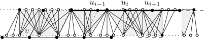
Figure 1: A fan-planar proper $2$-layer drawing and its graph (a stegosaurus).

Layered drawings are further distinguished by what types of edges are allowed; the following notation is from [11]. An edge is called flat if its endpoints lie on the same layer, proper if its endpoints lie on adjacent layers, and long otherwise. A proper ${h}$-layer drawing contains only proper edges, a short ${h}$-layer drawing contains no long edges, an upright ${h}$-layer drawing contains no flat edges, and an unconstrained ${h}$-layer drawing permits any type of edge. Any graph with a planar upright ${h}$-layer drawing has pathwidth at most $h$, and at most $h{-}1$ if there are no flat edges [5, 6]. Any graph with a fan-planar proper $2$-layer drawing is a subgraph of a so-called stegosaurus (see Fig. 1 and Section 5) [2]; those have pathwidth 2.

A key concept for us is where crossings can be in proper layered drawings and how to group them. Let $G_{P}$ be the planarization of some graph $G$ with a fixed embedding. As in Fig. 2, a crossing-patch $\mathcal{C}$ is a maximal connected subgraph of $G_{P}$ for which all vertices are crossing-dummy-vertices. Let $E_{\mathcal{C}}$ be the edges of $G$ that have crossings in $\mathcal{C}$, let $V_{\mathcal{C}}$ be the endpoints of $E_{\mathcal{C}}$, and let $G_{C}$ be the graph $(V_{C},E_{C})$. Since any edge connects two adjacent layers, and a crossing-patch is connected, we can observe:

Observation 1.

If $G$ has a proper embedding-preserving layered drawing $\Gamma$ then all crossings of a crossing-patch $\mathcal{C}$ lie strictly between two consecutive layers, and the vertices in $V_{\mathcal{C}}$ lie on those layers.

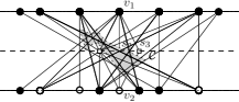
(a)  

(b)  

Figure 2: A crossing-patch in a graph that is not fan-planar, and how to contract it.

3 Bar-Visibility representations and Pathwidth

In this section, we show that a graph with a fan-planar short ${h}$-layer drawing has pathwidth at most $2h-1$ (and at most $2h-2$ if the drawing is proper). The proof uses a bar-$c$ visibility representation, which is an assignment of a horizontal line segment (bar) to every vertex and a vertical line segments connecting the bars of endpoints to every edge in such a way that bars are disjoint and every edge-segment contains at most $c$ points (not counting the endpoints) that belong to bars.

(a)  

(b)  

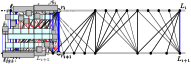
(c)  

(d)  

Figure 3: A fan-planar proper ${2}$-layer drawing; planar edges that separate fan-subgraphs are blue (thick). [For labelling-purposes we show the planar edges as vertex-disjoint, but consecutive ones could have vertices in common.] We show the four possible locations of center-vertices (white).

Theorem 3.1.

If $G$ has fan-planar proper ${h}$-layer drawing $\Gamma$, then $G$ has a bar-1-visibility representation. Moreover, any vertical line intersects at most $2h-1$ bars of the visibility representation.

Proof.

In the first step, make $\Gamma$ maximal, i.e., insert all edges that can be added while keeping a fan-planar proper ${h}$-layer drawing. In the resulting drawing every crossing-patch is enclosed by two planar edges (shown thick blue in Fig. 3). The subgraph between two such planar edges consists (if it has crossings at all) of two crossing fans; we call this a fan-subgraph. Studying all possible positions of these two fans, we see that the two center-vertices include exactly one of the top vertex of the left planar edge or the bottom vertex of the right planar edge. We remove the crossed edges incident to this center-vertex in the fan-subgraph; see Fig. 3 where removed edges are red (dashed). The remaining graph $G^{\prime}$ is planar and has a planar proper ${h}$-layer drawing. We can convert this into a bar-0-visibility representation $\Gamma^{\prime}$ where the layer-assignment and the order within layers is unchanged [1], in particular any vertical line intersects at most $h$ vertex-bars.

Next, shift bars upward until bars of each layer lie “diagonally”, see the dark gray bars in Fig. 4. More precisely, we process layers from bottom to top. For each layer we assign increasing $y$-coordinates to the bars from left to right such that every bar has its own $y$-coordinate.

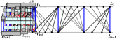
(a)  

(b)  

(c)  

(d)  

Figure 4: Bar-1-visibility representation for different types of fan-subgraphs.

Let the planar edges to the left and right of a fan-subgraph be $(\ell_{i},\ell_{i+1})$ and $(r_{i},r_{i+1})$, with vertices indexed by layer. The process of removing edges ensures that all of the missing edges are incident to $r_{i+1}$ or $\ell_{i}$. If they were incident to $\ell_{i}$, then we extend $\ell_{i}$ to the right until it vertically sees its diagonally opposite corner $r_{i+1}$. Otherwise, we extend $r_{i+1}$ to the left until it vertically sees its diagonally opposite corner $\ell_{i}$. This extension realizes all removed edges of the fan-subgraph, since the extended bar can see vertically all other bars of vertices of the fan-subgraph. By our construction, the extended bars do not cross the planar edges between $\ell_{i}$ and $\ell_{i+1}$, or between $r_{i}$ and $r_{i+1}$. Since for each fan-subgraph there is only one extended bar, the edges of $G$ that belong to $G^{\prime}$ go through at most one extended bar. Therefore the computed representation is a bar-1-visibility representation of $G$. In each fan-subgraph only one bar is extended, therefore every vertical line intersects at most $h$ bars from the $h$ layers and at most $h-1$ bars from the $h-1$ fan-subgraphs that it traverses. ∎

With a minor change, we can prove a similar result for short layered drawings.

Theorem 3.2.

If $G$ has a fan-planar short ${h}$-layer drawing $\Gamma$, then $G$ has a bar-1-visibility representation where any vertical line intersects at most $2h$ bars of the visibility representation.

Proof.

Let $G^{-}$ be the graph obtained by removing all flat edges; this has a fan-planar proper ${h}$-layer drawing and therefore a bar-1-visibility representation using Theorem 3.1. Let $\Gamma^{\prime}$ be the visibility representation (of some subgraph of $G^{-}$) used as intermediate step in this proof. Lengthen the bars of $\Gamma^{\prime}$ maximally so that within any layer, the bar of one vertex $v$ ends exactly where the bar of the next vertex $w$ begins. (Note that no vertical edge-segment lies between the bars of $v$ and $w$ since there are no long edges.) We have some choice in how much to extend $v$ vs. how much to extend $w$ into the gap between them, and do this such that no two points where bars begin/end have the same $x$-coordinate.

Now convert this visibility representation into a bar-1-visibility representation $\Gamma^{-}$ of $G^{-}$ exactly as before. We claim that this is the desired bar-1-visibility representation of $G$. Consider a flat edge $e=(v,w)$, with (say) $v$ left of $w$ on their common layer. Let $X_{e}$ be the $x$-coordinate where the bar of $v$ ends and the bar of $w$ begins in the modified $\Gamma^{\prime}$. To obtain $\Gamma^{-}$, these bars are first shifted to different $y$-coordinates (without changing $x$-coordinates of their endpoints). Since $v$ and $w$ are consecutive within one layer of $\Gamma^{\prime}$, they end of on consecutive layers of $\Gamma^{-}$. Next the bars are (possibly) lengthened, but never shortened. Therefore edge $(v,w)$ can be inserted with $x$-coordinate $X_{e}$ to connect the bars of $v$ and $w$.

It was argued in Theorem 3.1 that any vertical line intersects at most $2h-1$ bars in that construction. The only change in our construction is that sometimes endpoints of bars may have the same $x$-coordinate $X_{e}$ (for some flat edge $e$), which means that the vertical line with $x$-coordinate $X_{e}$ now may intersect more bars. However, we ensured that $X_{e}\neq X_{e^{\prime}}$ for any two flat edges $e,e^{\prime}$, which means that even at $x$-coordinate $X_{e}$ the vertical line intersects at most $2h$ bars. ∎

Corollary 1.

If $G$ has a fan-planar proper ${h}$-layer drawing, then $pw(G)\leq 2h-2$. If $G$ has a fan-planar short ${h}$-layer drawing, then $pw(G)\leq 2h-1$.

Proof.

Take the bar-1-visibility representation of $G$ from Theorem 3.1 [respectively 3.2] and read a path decomposition $\mathcal{P}$ from it. To do so, sweep a vertical line $\ell$ from left to right. Whenever $\ell$ reaches the $x$-coordinate of an edge-segment, attach a new bag $P$ at the right end of $\mathcal{P}$ and insert all vertices that are intersected by $\ell$. The properties of a path decomposition are easily verified since bars span a contiguous set of $x$-coordinates, and for every edge $(v,w)$ the line through the edge-segment intersects both bars of $v$ and $w$. Since any vertical line intersects at most $2h-1$ [$2h$, respectively] bars, each bag has size at most $2h-1$ [$2h$] and the width of the decomposition is at most $2h-2$ [$2h-1$]. ∎

We now show that the bounds of Corollary 1 are tight, even for trees.

Theorem 3.3.

For any $h\geq 1$, there are trees $T^{p}_{2h{-}2}$ and $T^{s}_{2h{-}1}$ such that

• $T^{p}_{2h{-}2}$ has a fan-planar proper ${h}$-layer drawing and $pw(T^{p}_{2h{-}2})\geq 2h{-}2$,

• $T^{s}_{2h{-}1}$ has a fan-planar short ${h}$-layer drawing and $pw(T^{s}_{2h{-}1})\geq 2h{-}1$.

Proof.

Roughly speaking, for $\alpha\in\{s,p\}$, $T_{i}^{\alpha}$ is the complete ternary tree with some (but not all) edges subdivided. To be more precise, for $h=1$, define $T_{0}^{p}$ to be a single node $r_{0}$, which can drawn on one layer and has pathwidth $0=2h-2$. Define $T_{1}^{s}$ to be an edge $(r_{1},\ell)$, which can be drawn as a flat edge on one layer and has pathwidth $1=2h-1$.

For $\alpha\in\{s,p\}$ and any $i$ where $T_{i}^{\alpha}$ is not yet defined, set $\overline{T}_{i}^{\alpha}$ to be a new vertex $r_{i}$ with three children, and make each child a root of $T_{i-1}^{\alpha}$. Clearly $pw(\overline{T}_{i}^{\alpha})\geq pw(T_{i-1}^{\alpha})+1$, since removing $r_{i}$ from $\overline{T}_{i}^{\alpha}$ gives three components that each contain $T_{i-1}^{\alpha}$. To obtain $T_{i}^{\alpha}$ from $\overline{T}_{i}^{\alpha}$ we subdivide some edges (see below). This cannot decrease the pathwidth, so using induction one shows that $pw(T_{i}^{\alpha})\geq i$.

Figure 5 shows that for all $i$ where $\overline{T}^{\alpha}_{i-2}$ is defined, $\overline{T}^{\alpha}_{i}$ has a fan-planar drawing with one more layer than used by $\overline{T}^{\alpha}_{i-2}$. Furthermore, $r_{i}$ is in the top row, and every edge is drawn properly, presuming we subdivide the edges incident to $r_{i}$. Using induction therefore $T_{2h-2}^{p}$ and $T_{2h-1}^{s}$ have fan-planar ${h}$-layer drawings. ∎

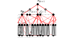
(a)  

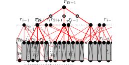
(b)  

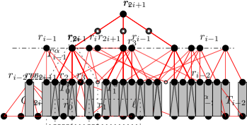
(c)  

Figure 5: (a) The trees for $h=1$. (b) Constructing $T^{\alpha}_{i}$ from $T^{\alpha}_{i-2}$ and (c) drawing it using one added layer.

Note that the drawing in Fig 5(c) are fan-planar, but not 1-planar. This naturally raises the question: What is the pathwidth of a graph that has a 1-planar ${h}$-layer drawing? We suspect that it cannot be more than $\approx\frac{3}{2}h$ (this remains open), and can show that for the above trees (subdivided differently) this bound would be tight.

Theorem 3.4.

For any odd $h\geq 1$ (say $h=2k+1$ with $k\geq 0$), there are trees $T^{p}_{3k}$ and $T^{s}_{3k{+}1}$ such that

• $T^{p}_{3k}$ has a 1-planar proper ${h}$-layer drawing and $pw(T^{p}_{3k}){\geq}3k=\frac{3}{2}h-\frac{3}{2}$, and

• $T^{s}_{3k{+}1}$ has a 1-planar short ${h}$-layer drawing and $pw(T^{s}_{3k{+}1})\geq 3k{+}1=\frac{3}{2}h-\frac{1}{2}$.

Proof.

Define $T_{0}^{p}$ and $T_{1}^{s}$ exactly as in the previous proof; their drawings have no crossings. Also define $\overline{T}^{\alpha}_{i}$ as before, but subdivide edges differently to obtain $T^{\alpha}_{i}$; see below. Figure 6 shows that $\overline{T}^{\alpha}_{i}$ has a 1-planar drawing with two more layers than $\overline{T}^{\alpha}_{i-3}$ (for all $i$ where $\overline{T}^{\alpha}_{i-3}$ is defined). Furthermore, $r_{i}$ is in the top row, and every edge is drawn properly, presuming we subdivide two edges incident to $r_{i}$ and all child-edges at the child $r_{i-1}$ whose parent-edge was not subdivided. The result now follows using induction on $h$. ∎

(a)  

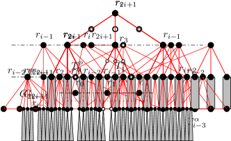
(b)  

Figure 6: (a) Constructing $T^{\alpha}_{i}$ from $T^{\alpha}_{i-3}$ and (b) drawing it using two added layers.

4 Testing Algorithm for Embedded Graphs

This section presents FPT-algorithms to determine whether an embedded graph $G$ has an embedding-preserving ${h}$-layer drawing. The first algorithm tests the existence of a proper drawing, and can be applied to fan-planar graphs. (In fact, the algorithm works for any embedded graph if we allow the order of crossings along an edge to change.) A minor change allows to test the existence of short drawings instead. For the smaller class of 1-planar graphs, yet another change allows to test the existence of an unconstrained drawing. All algorithms require crucially that the embedding is fixed.

Recall that Dujmović et al. [5] gave an algorithm for this problem for planar graphs where the embedding is not fixed; in the following we refer to their algorithm as PlanarDP. The idea for our algorithm is to convert $G$ into a planar graph $G^{\prime}$ such that $G$ has an embedding-preserving ${h}$-layer drawing if and only if $G^{\prime}$ has a plane ${h^{\prime}}$-layer drawing (where $h^{\prime}=2h{-}1$). One might be tempted to then appeal to PlanarDP. However, it is not at all clear whether PlanarDP could be modified to guarantee that the planar embedding is respected. We therefore further modify $G^{\prime}$ (in two steps) into a planar graph $G^{\prime\prime\prime}$ that has a planar ${h^{\prime\prime\prime}}$-layer drawing (where $h^{\prime\prime\prime}=12h^{\prime}{+}1$) if and only if $G^{\prime}$ has a plane ${h^{\prime}}$-layer drawing. Then call PlanarDP on $G^{\prime\prime\prime}$.

This latter step is of interest in its own right: For plane graphs, we can test the existence of a plane ${h}$-layer drawing in time FPT in $h$. This improve on PlanarDP, which permitted changes of the embedding.

To simplify the reductions, it is helpful to observe that PlanarDP allows further restrictions. This algorithm first computes a path decomposition $\mathcal{P}$ of small width. It then uses dynamic programming with table-entries indexed (among other things) by the bags of $\mathcal{P}$ and specifying (among other properties) the layer for each vertex in the bag. So we can impose restrictions on the layers that a vertex may be on. Also, since for any edge some bag contains both endpoints, we can impose restrictions on the span, i.e., the distance between the layers of its endpoints. We will impose even more complicated restrictions that require changing the path decomposition a bit; this will be explained below.

4.1 Proper drawings: Contracting Crossing Patches

This section applies when we want to test the existence of a proper ${h}$-layer drawing (i.e., no long or flat edges are allowed). We start with an easy lemma.

Lemma 1.

Let $G$ be an embedded graph with a crossing-patch $\mathcal{C}$, and assume $G$ has an embedding-preserving proper ${h}$-layer drawing $\Gamma$. Then in the embedding of $G_{\mathcal{C}}$ induced by the one of $G$, all vertices of $V_{\mathcal{C}}$ are on the infinite region.

Proof.

By Observation 1, the induced drawing of subgraph $G_{\mathcal{C}}$ lies entirely between two layers $L_{i}$ and $L_{i+1}$, with $V_{\mathcal{C}}$ on these layers and hence on the infinite region. Since the drawing is embedding-preserving, $V_{C}$ hence is on the infinite region of the induced embedding of $G_{\mathcal{C}}$. ∎

Note that the conclusion of Lemma 1 depends only on the embedding of $G$, not on $\Gamma$, and as such can be tested given the embedding of $G$. In the rest of this subsection we assume that it holds for all crossing-patches, as otherwise $G$ has no embedding-preserving proper layered drawing and we can stop.

As depicted in Fig. 2, the operation of contracting a crossing-patch $\mathcal{C}$ consists of contracting all the edge-segments within $\mathcal{C}$ to obtain one vertex $c$ that is adjacent to all of $V_{\mathcal{C}}$. Hence, the rotation at $c$ lists the vertices of $V_{\mathcal{C}}$ in the order in which they appeared on the infinite region of $G_{\mathcal{C}}$. As Fig. 2 suggests, we can convert a proper layered drawing $\Gamma$ of $G$ into a layered drawing $\Gamma^{\prime}$ of $G^{\prime}$ with roughly twice as many layers. To be able to undo such a conversion, observe that $\Gamma^{\prime}$ has special properties. First, it is 2-proper, by which we mean that for any edge $(v,w)$ of $G$ the vertices $v$ and $w$ are exactly two layers apart, and the edges incident to a contracted vertex $c$ are proper. It also preserves monotonicity: for any edge $(v,w)$ of $G$ that had a crossing, the edges $(v,c)$ and $(c,w)$ are drawn such that their union is a $y$-monotone curve. Since $G^{\prime}$ is obtained from $G$ by contracting crossing-patches, and each contracted vertex $c$ can be placed at a dummy-layer between the two layers surrounding the crossing-patches, one immediately verifies:

Lemma 2.

Let $G$ be an embedded graph, and let $G^{\prime}$ be the graph obtained by contracting crossing-patches. If $G$ has an embedding-preserving proper ${h}$-layer drawing $\Gamma$ then $G^{\prime}$ has a plane monotonicity-preserving 2-proper ${(2h{-}1)}$-layer drawing.

The other direction is not obviously true. It is easy to convert a plane monotonicity-preserving 2-proper ${(2h{-}1)}$-layer drawing of $G^{\prime}$ to an ${h}$-layer drawing of $G$ with the correct rotation system and pairs of crossing edges (the drawing is weakly isomorphic [10]). But the order of crossings may change when connecting vertices by straight-line segments. For example, in Fig. 2(a), moving the top left vertex much farther left would change the order of crossings while keeping the rotation scheme unchanged. So we give the other direction only for fan-planar graphs, where this is impossible.

Lemma 3.

Let $G$ be a fan-plane graph, and let $G^{\prime}$ be the graph obtained by contracting crossing-patches. If $G^{\prime}$ has a plane monotonicity-preserving 2-proper ${(2h{-}1)}$-layer drawing $\Gamma^{\prime}$ then $G$ has a fan-plane proper ${h}$-layer drawing.

Proof.

Consider any crossing patch $\mathcal{C}$ of $G$ that was contracted into vertex $c$, say $c$ is on layer $L_{i}$ in $\Gamma^{\prime}$. Since the drawing is 2-proper, all neighbours of $c$ are on $L_{i-1}$ or $L_{i+1}$. Since for any edge $(v,w)$ in $E_{\mathcal{C}}$ the endpoints are two layers apart, therefore $v\in L_{i-1}$ and $w\in L_{i+1}$ or vice versa. Remove the edges incident to $c$ and re-insert the edges in $E_{\mathcal{C}}$ as straight-line segments.

Since the rotation at $c$ is respected, the order of $V_{\mathcal{C}}$ on $L_{i-1}\cup L_{i+1}$ reflects the order along the infinite region of $G_{\mathcal{C}}$. Two edges $e,e^{\prime}$ in $E_{\mathcal{C}}$ crossed in $G$ if and only if their endpoints alternated in the order along the infinite region of $G_{\mathcal{C}}$, and so they cross in the resulting drawing as needed.

Assume an edge $e=(u,w)$ in $E_{\mathcal{C}}$ crosses edges $e_{1},\dots,e_{d}$ in $G$, in this order while walking from $u$ to $w$. It suffices to argue that the same order of crossings happens in the created drawing. Let $v$ be the common endpoint of $e_{1},\dots,e_{d}$, say $e_{i}=(v,w_{i})$ for $i=1,\dots,d$. We know that endpoints of $e,e_{1},\dots,e_{d}$ are on the infinite region of $G_{\mathcal{C}}$ since they belong to $V_{\mathcal{C}}$. Furthermore, their (clockwise or counter-clockwise) order along the infinite region must be exactly $v,u,w_{1},\dots,w_{d},w$ since we have a good drawing. Namely, for any $i\in 1,\dots,d$ vertex $v$ must be separated from $w_{i}$ in the order by $\{u,w\}$, otherwise $e$ and $e_{i}$ would have to cross twice since they cross at least once. Also, for any $i<j$, if the order along the infinite region is $u,w_{j},w_{i},v$ while the order along $e$ is $u,e_{i},e_{j},v$, then $e_{j}$ and $e_{i}$ would have to cross each other between where they cross $e$ and their endpoints $w_{i}$ and $w_{j}$. In a good drawing no two edges cross twice and edges with a common endpoint do not cross, so both are impossible.

Assume up to symmetry that $v\in L_{i-1}$, which means that $w_{1},\dots,w_{d}$ are on $L_{i+1}$. Since the rotation at $c$ contains $v,u,w_{1},\dots,w_{d},w$ in this order, $w_{1},\dots,w_{d}$ are on layer $L_{i+1}$ in this order, and edge $e$ crosses $e_{1},\dots,e_{d}$ in this order as desired.

Repeating this operation at all crossing patches hence gives a drawing of $G$ that respects the embedding. After deleting even-indexed layers (which contained no vertices of $G$), we obtain a fan-plane proper ${h}$-layer drawing of $G$. ∎

4.2 Flat and long edges

We will discuss in a moment how to test whether a graph has a plane ${(2h{-}1)}$-layer drawing that is monotonicity-preserving and 2-proper, but first study modifications that allow us to test for short drawings (i.e., to allow flat edges) and unconstrained drawings.

Only minimal changes are needed when flat edges are allowed. Observation 1, and therefore Lemma 1 continue to hold. When there are no long edges, flat edges never have crossings. So it suffices to allow edges without crossings to have span 0 in $G^{\prime}$. We say that a layered drawing $\Gamma^{\prime}$ of $G^{\prime}$ is 2-short if for any edge $(v,w)$ of $G$ the vertices $v,w$ are either zero or two layers apart, and the edges incident to a contracted vertex $c$ are proper.

Lemma 4.

Let $G$ be a fan-plane graph, and let $G^{\prime}$ be the graph obtained by contracting crossing-patches. $G$ has a fan-plane short ${h}$-layer drawing if and only if $G^{\prime}$ has a plane monotonicity-preserving 2-short ${(2h{-}1)}$-layer drawing.

Proof.

The forward-direction is straightforward. The backward direction is proved almost exactly as in Lemma 3, except that preserving monotonicity is now vital (while it was not actually needed in Lemma 3). Namely, if $(v,w)$ is an edge involved in some crossing-patch that was contracted to vertex $c$, then a 2-short drawing permits $v$ and $w$ to be on the same layer, e.g. both above the layer $L_{i}$ of $c$. But monotonicity-preserving (and proper edges incident to $c$) force them to be on layers $L_{i-1}$ and $L_{i+1}$ instead and the rest of the proof can proceed as before. ∎

Long edges pose difficulties because Observation 1 no longer holds. However, in a 1-plane graph $G$ every crossing-patch has a single crossing, i.e., contracting crossing-patches is simply planarizing $G$. This crossing therefore either lies between two layers or (if a long edge crosses a flat edge) exactly on a layer. Define a drawing of $G^{\prime}$ to be 2-unconstrained if every vertex of $G$ lies on an odd-indexed layer. The following is shown almost exactly as Lemma 2-4; we leave the details to the reader.

Lemma 5.

Let $G$ be a 1-plane graph and let $G^{\prime}$ be its planarization. Then $G$ has a 1-plane unconstrained ${h}$-layer drawing if and only if $G^{\prime}$ has a plane monotonicity-preserving 2-unconstrained ${(2h{-}1)}$-layer drawing.

4.3 Enforcing a rotation scheme

Recall that we want a plane drawing of $G^{\prime}$ while PlanarDP tests the existence of planar drawings. As the next step we hence turn $G^{\prime}$ into a graph $G^{\prime\prime}$ that is a subdivision of a 3-connected planar graph (hence has a unique planar rotation scheme). There are many ways of making a planar graph 3-connected (e.g. we could triangulate the graph or stellate every face), but we need to use a technique here that allows to relate the height of layered drawings of $G^{\prime}$ and $G^{\prime\prime}$, and this seems hard when using triangulation or stellation.

Instead we use a different idea, which is easier to describe from the point of view of angles of $G^{\prime}$, i.e., incidences between a vertex $v$ and a region $f$. (A vertex may be incident to a face repeatedly, in case of which this gives rise to multiple angles, but it should be clear from the context which of them we mean.) The operation of filling the angles of $G^{\prime}$ consists of two steps. First, replace every edge $e$ of $G^{\prime}$ by a tripler-graph $H$ ; $H$ consists of three (subdivided) copies of $e$ with some edges added to make $H$ an inner triangulation (see Fig. 7(b)). Now add a filler path at every angle $v,f$ of $G^{\prime}$ as follows. Let $u,w$ be the clockwise/counter-clockwise neighbour of $v$ on $f$ in $G^{\prime}$. Let $(v,u^{\prime})$ and $(v,w^{\prime})$ be the edges of the tripler-graphs of $(v,u)$ and $(v,w^{\prime})$ that are now on $f$. Add a subdivided edge between $u^{\prime}$ and $w^{\prime}$ and place it inside face $f$.

(a)  

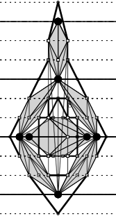
(b)  

(c)  

Figure 7: (a) A very small plane graph $G^{\prime}$. (b) Replacing a proper, flat or long edge with a tripler-graph. (c) Graph $G^{\prime\prime}$ obtained by filling all angles. Some edges from the tripler-graphs are not shown.

Lemma 6.

Let $G^{\prime}$ be a plane graph. Let $G^{\prime\prime}$ be a graph obtained by filling the angles of $G^{\prime}$. Then $G^{\prime\prime}$ is a subdivision of a 3-connected planar graph.

Proof.

Let $G_{c}$ be the graph obtained from $G^{\prime\prime}$ by contracting filler-paths into edges; we claim that $G_{c}$ is 3-connected. We can view $G_{c}$ as having been built as follows: Start with graph $G^{\prime}$ and subdivide every edge. For every face $f$ of degree $k$ of $G^{\prime}$, insert a cycle $C_{f}$ of length $2k$ inside $f$, and connect the vertices of $C_{f}$ to their corresponding vertices on $f$. Add a few more edges connecting $C_{f}$ to $f$ such that all faces except $C_{f}$ become triangles. In particular, all faces of $G_{c}$ are simple cycles, which immediately shows that $G_{c}$ is 2-connected. Also note that every vertex is incident to at most one non-triangular face, and for every edge at most one endpoint is incident to a non-triangular face. Now assume we have a cutting pair $\{v,w\}$, which means that at least two faces contain both $v$ and $w$. At least one of these faces must be a triangle, which means that $(v,w)$ is an edge. But then all faces incident to both $v$ and $w$ must be triangles, by the above condition on edges. This is impossible if $\{v,w\}$ is a cutting pair in a simple planar graph. ∎

Recall that we had some restrictions on drawings of $G^{\prime}$, such as being 2-proper and monotonicity-preserving. All of them can be expressed as a subgraph-restriction, where we are given a (connected, constant-sized) subgraph $H$ of $G^{\prime}$ and restrict the indices of layers used by $V(H)$. For example if $H$ is a single vertex, then we can force its layer to be among a set of layers of our choice. If it is a single edge then we can force its span to be among a set of spans of our choice. If $H=v$-$c$-$w$ for some contracted vertex $c$ and edge $(v,w)$ in $G$, then we can force $c$ to be within the range of the layers of $v,w$, hence $(v,c)\cup(c,w)$ is drawn $y$-monotonically. So this covers all the restrictions we had on $G^{\prime}$. We will discuss below how to test (under some assumptions) the existence of a subgraph-restricted ${h}$-layer drawing using PlanarDP.

So assume graph $G^{\prime}$ comes with some subgraph-restrictions $H_{1},\dots,H_{d}$. For $j=1,\dots,d$, translate restriction $H_{j}$ to $G^{\prime\prime}$ by letting $H_{j}^{\prime}$ be graph $H_{j}$ with edges replaced by tripler-subgraphs, and layer-restrictions replaced according to $i\leftrightarrow 3i{-}2$. We impose further subgraph-restrictions on $G^{\prime\prime}$: (1) Every vertex of $G^{\prime}$ of must be on a layer whose index is $2\bmod 3$, and (2) any tripler-graph $H$ must be drawn such that the middle path (the path between vertices of $G^{\prime}$ that uses no edges from the outer-face) is drawn $y$-monotonically.

Lemma 7.

Let $G^{\prime}$ be a plane graph. Let $G^{\prime\prime}$ be a graph obtained by filling the angles of $G^{\prime}$. Then $G^{\prime}$ has a plane subgraph-restricted ${h}$-layer drawing if and only if $G^{\prime\prime}$ has a plane subgraph-restricted ${(3h)}$-layer drawing.

Proof.

Assume first that $G^{\prime\prime}$ has a plane subgraph-restricted ${(3h)}$-layer drawing $\Gamma^{\prime\prime}$. The vertices of $G^{\prime}$ occur only every third layer, and the middle path of each tripler-graph is drawn $y$-monotonically. Hence after deleting filler-paths and tripler-graphs except for the middle paths, we obtain a drawing of $G^{\prime}$ on $h$ layers, with edges $y$-monotone since middle paths are $y$-monotone. The subgraph-restrictions of $G^{\prime}$ are satisfied since they were translated suitably into $G^{\prime\prime}$.

Now assume that $G^{\prime}$ has a plane subgraph-restricted ${h}$-layer drawing $\Gamma^{\prime}$, and insert a dummy-layer before and after any layer of $\Gamma^{\prime}$ to obtain $3h$ layers. Insert tripler-graphs in place of their corresponding edges using the appropriate drawing from Fig. 7. Clearly all subgraph-restrictions are satisfied. It remains to argue how to place filler-paths. Consider a face $f$ of $G^{\prime}$ containing a path $u$-$v$-$w$ in clockwise order; we filled the angle $v,f$ with filler-path $u^{\prime}$-$s$-$w^{\prime}$ where $s$ is a degree 2 vertex. Observe that $(v,u^{\prime})$ and $(v,w^{\prime})$ are drawn proper, regardless of the chosen drawing of the tripler-graphs. This puts $u^{\prime}$ and $w^{\prime}$ either on the same layer or two layers apart. Walking from $u^{\prime}$ to $w^{\prime}$ along face $f$ hence requires at most one bend, so we can draw the filler-path (with $s$ at the bend) such that all edges are $y$-monotone. See Fig. 7(c). ∎

4.4 Enforcing the outer-face

We do one more modification to enforce the outer-face. Let $G^{\prime\prime}$ be a graph that is a subdivision of a 3-connected planar graph $G_{c}$; we assume throughout that $G^{\prime\prime}$ is not a simple cycle since no simple cycle would arise from the prior modifications. The operation of adding escape-paths assumes that we are given one face $f$ of $G^{\prime\prime}$ (the desired outer-face) and consists of the following. Add a new vertex $r$ inside $f$. Pick three vertices $z_{1},z_{2},z_{3}$ on face $f$ that were also vertices in the 3-connected graph $G_{c}$; in particular $f$ is the only face that contains all three of them. Add three paths of length $n=|(V(G^{\prime\prime})|$ that connect $z_{1},z_{2},z_{3}$ to $r$; we call these the escape-paths.

Graph $G^{\prime\prime}$ may have subgraph-restrictions, which we translate to the resulting graph $G^{\prime\prime\prime}$ by changing layer-restrictions according to $i\leftrightarrow 4i{-}2$. We impose further subgraph-restrictions on $G^{\prime\prime\prime}$: Vertex $r$ is on the bottommost layer, and any vertex of $G^{\prime\prime}$ is on $L_{4i-2}$ for some $i\geq 1$.

Lemma 8.

Let $G^{\prime\prime}$ be a planar graph that is a subdivision of a 3-connected graph, embedded with face $f$ as the outer-face. Let $G^{\prime\prime\prime}$ be the graph obtained by adding escape-paths to $G^{\prime\prime}$. Then $G^{\prime\prime}$ has a plane subgraph-restricted ${h}$-layer drawing if and only if $G^{\prime\prime\prime}$ has a planar subgraph-restricted ${(4h{+}1)}$-layer drawing .

Proof.

If $G^{\prime\prime\prime}$ has a planar ${(4h{+}1)}$-layer drawing $\Gamma^{\prime\prime\prime}$ that satisfies the restrictions, then $r$ is on the bottommost layer, hence on the outer-face of $\Gamma^{\prime\prime\prime}$. Remove $r$ and the escape-paths to get the induced drawing $\Gamma^{\prime\prime}$ of $G^{\prime\prime}$; this must have $z_{1},z_{2},z_{3}$ on the outer-face since they are adjacent (via the escape-paths) to $r$. So the outer-face of $\Gamma^{\prime\prime}$ must be $f$. The rotation scheme of $G^{\prime\prime}$ is automatically respected since it is unique. Finally vertices of $G^{\prime\prime}$ only on every fourth layer, so by deleting all other layers we get a plane ${h}$-layer drawing of $G^{\prime\prime}$. This satisfies the restrictions on $G^{\prime\prime}$ since they were inherited into $G^{\prime\prime\prime}$.

Vice versa, if $G^{\prime\prime}$ has a plane ${h}$-layer drawing $\Gamma^{\prime\prime}$, then insert three layers between any two layers of $\Gamma^{\prime\prime}$, and also three layers above and one layer below $\Gamma^{\prime\prime}$. Place $r$ in the topmost layer. Clearly all subgraph-restrictions are satisfied, except that we need to explain how to route the escape-paths.

Vertices $z_{1},z_{2},z_{3}$ are on the outer-face $f$ of $\Gamma^{\prime\prime}$, which also contains $r$. Find, for $i=1,2,3$, a Euclidean shortest path $\pi_{i}$ from $z_{i}$ to $r$ inside $f$. (These three paths may overlap each other, but they do not cross.) Now place the escape-paths by tracing near $\pi_{i}$, but using the nearest available layer inside face $f$ instead. This is feasible, even at a local minimum or maximum of $\pi_{i}$, since only every fourth layer of $\Gamma^{\prime\prime\prime}$ contains vertices of $G^{\prime\prime}$, and only those vertices can be local minima/maxima. Therefore, even if all three paths $\pi_{1},\pi_{2},\pi_{3}$ go through one local minimum/maximum, we can still use the three layers below/above it to place bends for the escape-paths. See Fig. 8. These layers have not been used for other bends of escape-paths already since $\pi_{i}$ was a Euclidean shortest path.

At each local minimum or maximum the drawing $\Gamma_{i}$ of the escape-path to $z_{i}$ must use a vertex of degree 2 to ensure that edges are drawn $y$-monotonically. There are at most $\deg(f)\leq n-1$ such vertices, so there are sufficiently many degree-2 vertices in the escape-paths. If we did not use them all, then artificially add more vertices at bends or insert flat edges to use them up. See Fig. 8. Thus we can insert the escape-paths into the drawing and obtain the desired planar proper ${(4h{+}3)}$-layer drawing of $G^{\prime\prime\prime}$. ∎

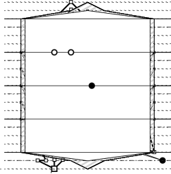
Figure 8: Routing the escape-paths (thick solid) along the outer-face. For illustration purposes we chose paths that are longer than needed.

4.5 Putting it all together

Theorem 4.1.

There are $O(f(h)poly(n))$ time algorithms of to test the following:

• Given a fan-plane graph $G$, does it have a fan-plane proper ${h}$-layer drawing?

• Given a fan-plane graph $G$, does it have a fan-plane short ${h}$-layer drawing?

• Given a 1-plane graph $G$, does it have a 1-plane unconstrained ${h}$-layer drawing?

Proof.

First test whether the conclusion of Lemma 1 is satisfied for all crossing-patches (this is trivially true for 1-planar graphs). If not, abort. Otherwise contract the crossing-patches of $G$ to obtain $G^{\prime}$, and add the subgraph-restrictions that $G^{\prime}$ must be drawn monotonicity-preserving and 2-proper/2-short/2-unconstrained. Fill the angles of $G^{\prime}$ to obtain $G^{\prime\prime}$, and add escape paths to obtain $G^{\prime\prime\prime}$. Inherit the above subgraph-restrictions into $G^{\prime\prime}$ and $G^{\prime\prime\prime}$. Also add the restrictions discussed when building $G^{\prime\prime}$ and $G^{\prime\prime\prime}$. We have argued that $G^{\prime\prime\prime}$ contains a planar subgraph-restricted ${(24h{-}11)}$-layer drawing if and only if $G$ has the desired embedding-preserving ${h}$-layer drawing.

We can test for the existence of a planar ${(24h{-}11)}$-layer drawing of $G^{\prime\prime\prime}$ using PlanarDP, the dynamic programming algorithm from [5]. (As this algorithm is quite complicated, we will treat it as a black box and not review it here.) As we argue now, in the same time we can also ensure the created subgraph-restrictions $H_{1},\dots,H_{d}$. Observe that every edge of $G^{\prime\prime\prime}$ belongs to a constant number of subgraph-restrictions, and that each $H_{j}$ has constant size. Let $\mathcal{P}$ be a path decomposition of $G^{\prime\prime\prime}$ of width at most $24h$ (this must exist, otherwise $G^{\prime\prime\prime}$ has no ${(24h{-}11)}$-layer drawing). $\mathcal{P}$ is found as part of PlanarDP. Modify $\mathcal{P}$ as follows: For each $H_{j}$ that is not a single vertex, and every bag $P$ that contains at least one edge of $H_{j}$, add all vertices of $H_{j}$ to $P$. The result $\mathcal{P}^{\prime}$ is a path decomposition since $H_{j}$ is connected. Since bag $P$ represents $O(h)$ edges (it induces a planar graph), and edges belong to constant number of restriction subgraphs of constant size, the bags of $\mathcal{P}^{\prime}$ have size $O(h)$. Call PlanarDP on $G^{\prime\prime\prime}$ using this path decomposition $\mathcal{P}^{\prime}$. Since each table-entry of the dynamic program specifies the layer-assignment, and since each restriction subgraph $H_{j}$ appears in at least one bag $P$ of $\mathcal{P}^{\prime}$, we can enforce the subgraph-restriction by permitting (among the table-entries indexed by bag $P$) only those that satisfy the restriction on $H_{j}$. ∎

Sadly, our results are mostly of theoretical interest. Algorithm PlanarDP is FPT in $h$, but the dependency $f(h)$ on $h$ is a very large function. Our algorithm (where $h$ gets replaced by $24h$ and then increased by another constant factor to accommodate the subgraph-restrictions) makes this even larger.

5 Testing Algorithm for $2$-Layer Fan-planarity

Finally we turn to fan-planar drawings when the embedding is not fixed. We have results here only for 2 layers (which are surprisingly complicated already). Graphs with maximal fan-planar proper $2$-layer drawings have been studied earlier by Binucci et al. [2]. They characterized these graphs as subgraphs of a stegosaurus (illustrated in Fig. 1; we review its definition now).

A ladder is a bipartite outer-planar graph consisting of two paths of the same length $\langle u_{1},u_{2},\dots,u_{\frac{n}{2}}\rangle$ and $\langle v_{1},v_{2},\dots,v_{\frac{n}{2}}\rangle$, called upper and lower paths, plus the edges $(u_{i},v_{i})$ $(i=1,2,\dots,\frac{n}{2})$; the edges $(u_{1},v_{1})$ and $(u_{\frac{n}{2}},v_{\frac{n}{2}})$ are called the extremal edges of the ladder. A snake is a planar graph obtained from an outer-plane ladder, by adding, inside each internal face, an arbitrary number (possibly none) of paths of length two connecting a pair of non-adjacent vertices of the face. In other words, a snake is obtained by merging edges of a sequence of several $K_{2,h}$ ($h\geq 2$). We may denote the partite set with more than 2 vertices (if any) the large side of a $K_{2,h}$. A vertex of a snake is mergeable if it is an end-vertex of an extremal edge and belongs to the large side of an original $K_{2,h}$. Mergeable vertices are black in Fig. 1. A stegosaurus is a graph obtained by iteratively merging two snakes at a distinct mergeable vertex, and by adding degree-1 neighbors (“stumps”) to mergeable vertices. We call a vertex of degree 2 in a stegosaurus a joint vertex; these are on the large side of a $K_{2,h}$. Note that each ladder vertex has either three or four ladder vertices as neighbors, except for the vertices at extremal edges. If a ladder vertex has four neighboring ladder vertices, then it is a cut-vertex in $G$. Binucci et al. [2] showed that a graph is fan-planar proper $2$-layer if and only if it is a subgraph of a stegosaurus. Recognizing snakes (which are exactly the biconnected fan-planar proper $2$-layer graphs) is polynomial [2], but the complexity of recognizing fan-planar proper $2$-layer graphs that are not biconnected is open.

Now we show how to test whether a tree has a fan-planar proper $2$-layer.

Theorem 5.1.

Let $T$ be a tree with $n$ vertices. We can test in $O(n)$ time whether $T$ admits a fan-planar proper $2$-layer drawing.

Proof.

Suppose that $T$ is fan-planar proper $2$-layer and let $G$ be a stegosaurus such that $T\subset G$. All stumps in $G$ are leaves in $T$. Let $T^{\prime}$ be the tree obtained from $T$ by removing all its leaves; then $T^{\prime}$ contains no stumps. We use the term leafless for a vertex of $T^{\prime}$ that was not incident to any leaves of $T$. We need some straightforward observations.

Claim.

In $T^{\prime}$, a ladder vertex $v$ of $G$ is adjacent to at most two joint vertices, and if it is incident to two joint vertices $y,y^{\prime}$ then they belong to distinct $K_{2,h}$.

Proof.

If $v$ is incident to three joint vertices then two of them are in the same $K_{2,h}$, so we only need to show the second claim. Recall that $y,y^{\prime}$ have degree 2 in $G$ and (since they are in $T^{\prime}$) also have degree 2 in $T$. So the edges to their other common neighbour $z$ in the $K_{2,h}$ must also be in $T$, giving us a cycle $v_{i}$-$y$-$z$-$y^{\prime}$ in $T$, an impossibility. ∎

Claim.

$T^{\prime}$ contains no vertex with degree greater than four.

Proof.

Assume for contradiction that (up to symmetry) $v_{i}$ has 5 neighbours in $T^{\prime}$. We claim that nearly always the situation of the previous claim must happen and consider cases. If $v_{i}$ was a mergeable endvertex of a snake then it had at most 4 neighbours that are not stumps (hence potentially in $T^{\prime}$). If $v_{i}$ was an endvertex of a snake but not mergeable, then it belongs to only one $K_{2,n}$ and has at most 2 neighbours of degree 3 or more, so the above situation applies. So we are done unless $v_{i}$ is in the middle of a snake, and its two incident $K_{2,h}$-subgraphs (which share edge $(v_{i},u_{i})$ in $G$) contain exactly one joint-vertex each while the other three neighbours of $v_{i}$ in $T^{\prime}$ are $v_{i-1},u_{i}$ and $v_{i+1}$. Call the two joint-vertices $x_{i-1}$ and $x_{i+1}$ (connected to $u_{i-1}$ and $u_{i+1}$). As before, edges $u_{i-1}$-$x_{i-1}$-$v_{i}$-$x_{i+1}$-$u_{i+1}$ all must exist in $T$. But then $u_{i}$ can only be connected to $v_{i}$ in $T$, because its only other incident edge $(u_{i},u_{i-1})$ and $(u_{i},u_{i+1})$ would lead to a cycle in $T$. Therefore $u_{i}$ has degree 1 in $T$ and is not in $T^{\prime}$, a contradiction. ∎

The idea now is to test whether $T^{\prime}$ (and hence $T$) can be augmented to a stegosaurus $G$ (without stumps). Let $\Pi=\langle u_{1},u_{2},\dots,u_{l}\rangle$ be the longest path of $T^{\prime}$. The vertices of $\Pi$ with degree greater than two represent ladder vertices of $G$ whose subtrees must be “paired” with corresponding sub-paths in $\Pi$ in order to reconstruct $G$.

We assign a type to each node $u_{i}$ of $\Pi$ as follows. If $u_{i}$ has degree four, it is of type A. If $u_{i}$, with $1<i<l$, has degree two and is leafless, and both $u_{i-1}$ and $u_{i+1}$ have degree three, then $u_{i-1}$, $u_{i}$, and $u_{i+1}$ are of type B and form a triple. If $u_{i}$ has degree three (and it is not of type B), it is of type C. If $u_{i}$ has degree two (and it is not of type B), it is of type D. Call a subtree of $T^{\prime}$ primary if it contains a vertex of $\Pi$, and secondary otherwise.

Figure 9: Showing the longest path of $T^{\prime}$ (bold) and the case in which a secondary subtree rooted at a type-A vertex $u_{i}$ contains a vertex of degree greater than two. The dotted edges are those missing to reconstruct a putative ladder containing the secondary subtree.

Claim.

If $u_{i}$ is of type $A$, then no secondary subtree rooted at $u_{i}$ contains a vertex of degree 3 in $T^{\prime}$.

Proof.

If $u_{i}$ is of type A, there are two primary and two secondary subtrees rooted at $u_{i}$. Observe that $u_{i}$ is a cut-vertex vertex of $G$, that is, there are two snakes in $G$ that were merged at $u_{i}$. Then each secondary subtree of $u_{i}$ is a path that belongs to one of these two snakes. To see this, recall that $T^{\prime}$ contains no stumps of $G$ and that each ladder vertex of $G$ is adjacent to at most one joint vertex in $T^{\prime}$. Hence, a vertex $v$ of degree greater than two is adjacent to either three ladder vertices or two ladder vertices and one joint. In both cases, vertex $v$ cannot belong to a secondary subtree as it would contain a path longer than the longest path in one of the two primary subtrees, see Fig. 9 for an illustration. ∎

If $u_{i-1}$, $u_{i}$, and $u_{i+1}$ are a triple of type B, with a similar argument one can prove that the secondary subtree rooted at $u_{i-1}$ and that the secondary subtree at $u_{i+1}$ are both paths.

If $u_{i}$ is of type C, then its secondary subtree may contain at most one vertex $v$ of degree greater than two, namely, such a vertex (if any) has degree three and it is either directly adjacent to $u_{i}$ or there is one degree-2 node between $u_{i}$ and $v$. Again, this is implied by the fact that a vertex of degree greater than two is a ladder vertex and that a secondary subtree cannot contain a sub-path whose length is longer than the longest path in one of the two primary subtrees of $u_{i}$.

If $u_{i}$ is of type D, there is no secondary subtree rooted at $u_{i}$.

The idea is now to use a greedy strategy along the nodes of $\Pi$ starting from $u_{1}$ in order to reconstruct a stegosaurus $G$ containing $T^{\prime}$. Recall that a stegosaurus is composed of distinct snakes, each having an underlying ladder. Hence, we can view all upper (lower) paths of these ladders as a unique upper (lower) path that goes through extremal edges. Without loss of generality, we assign $u_{1}$ to be the first ladder vertex of the upper path of $G$. While we extend the path $\Pi$ from left to right on either the upper or lower path, we keep track of an integer offset variable that stores the minimum required number of ladder vertices on the respective other ladder path. This offset can take positive and negative values, depending on whether the other path extends beyond the currently considered node $u_{i}$ of $\Pi$ or not. For negative offsets the considered primary node extends further to the right than the last node on the other ladder path, while for positive offsets the primary path lags behind. An offset of $0$ means that both ladder paths extend equally far. Let $o_{i}$ be this offset value corresponding to node $u_{i}$.

Furthermore we need to store a flag $\beta_{i}$ with each offset $o_{i}$ that expresses whether ($\beta_{i}=1$) or not ($\beta_{i}=0$) at least one leafless node exists on the ladder path opposite of $\Pi$ in the currently extended snake. By default each flag is set to 0. This information is required in some extremal cases for deciding if all leaves can be re-inserted in the end of the process or not. In fact, the existence of a single leafless node on a ladder in which all ladder vertices are contained in $T^{\prime}$ guarantees that all other nodes of $T^{\prime}$ on this ladder can have arbitrarily many leaves. However, the existence of a leafless node on the ladder path is only beneficial if the choice is between two options with identical offsets. Otherwise the smaller offset option will always allow for strictly more freedom when continuing to extend the primary path $\Pi$.

For each node $u_{i}$ of $\Pi$, we distinguish all possible cases based on its type. Node triples of type-B are considered together in one step. We assume that the primary subtree that contains $u_{i-1}$ has already been processed by the algorithm. Without loss of generality we can assume that $u_{i-1}$ is part of the upper path of $G$; otherwise we simply flip the roles of the upper and lower path. While, depending on the type of $u_{i}$, there are many options of distributing the primary subtree containing $u_{i+1}$ and the secondary subtrees, we observe that (i) it is sufficient to consider the primary path going monotonically from left to right and (ii) if several options are valid it is sufficient to select the one yielding the smallest offset $o_{i}$, and in case of ties one with $\beta_{i}=1$. This is because the smaller an offset and the more leafless nodes on the secondary path, the more freedom we maintain for placing future secondary paths. Additionally, in a stegosaurus, any decision for a type-A, -B, or -C node $u_{i}$ only depends on the offset $o_{i-1}$ and the flag $\beta_{i-1}$ of its predecessor $u_{i-1}$ on $\Pi$ and the length of its secondary subtree(s). Hence we can greedily select among all feasible options the one producing smallest offset $o_{i}$ and as a tie-breaker a larger value $\beta_{i}$. For ease of presentation, we discuss the types in the order A,C,D, and finally B.

Type A. If $u_{i}$ is of type A, we have four options of embedding the primary subtree containing $u_{i+1}$ and the two secondary subtrees, see Fig. 10. Recall that $u_{i}$ is a cut node of $G$ and thus there are two snakes (and hence ladders) that meet at $u_{i}$. Let $s_{1}$ and $s_{2}$ be the two secondary subtrees, which are in fact paths. Let $|s_{1}|$ and $|s_{2}|$ denote their lengths and assume $|s_{1}|\leq|s_{2}|$. If $o_{i-1}+|s_{2}|-1\leq 0$ then there is enough space in the ladder of $u_{i-1}$ to assign $s_{2}$ (or $s_{1}$) to be part of its lower path. In this case it is better to assign $s_{2}$ to the left ladder as this yields the smaller offset $o_{i}$ (compare Fig. 10(a) and (c) or Fig. 10(b) and (d)). If the condition on the length of $s_{2}$ is satisfied with equality, we need to additionally check that $\beta_{i-1}=1$ or that the secondary path embedded to the left has a leafless node – else we have to reject the instance. Otherwise, if $o_{i-1}+|s_{2}|-1>0$ but $o_{i-1}+|s_{1}|-1\leq 0$ then $s_{1}$ must be part of the left ladder (see Fig. 10(a–b)) and we again need to verify the existence of a leafless node on the ladder path in case of equality. In either case, we obtain a smaller offset $o_{i}$ if the primary path stays on the upper path of $G$ (compare Fig. 10(a–b) or Fig. 10(c–d)). Thus we set $o_{i}=|s_{1}|-1$ if $s_{1}$ is embedded to the right, or $o_{i}=|s_{2}|-1$ if $s_{2}$ is embedded to the right. We set $\beta_{i}=1$ if the path embedded to the right has a leafless node. If, however, $o_{i-1}+|s_{1}|-1>0$ then we cannot embed either secondary path into the left ladder and thus report that $T^{\prime}$ is no subgraph of a stegosaurus $G$.

Figure 10: Different possibilities of embedding $T^{\prime}$ for a node $u_{i}$ of type A.

Type C. If $u_{i}$ is of type C we distinguish two sub-cases depending on whether the secondary tree $s$ rooted at $u_{i}$ is a path or not. We first consider that $s$ is a path, see Fig. 11(a–d). In the general case that any vertex of $s$ may have leaves in $T$ and thus needs to be embedded as a ladder vertex we have two options (Fig. 11(a–b)). If $o_{i-1}+|s|-1\leq 0$ then we can embed $s$ into the left ladder (modulo the existence of a leafless node in case of equality) and set $o_{i}=-1$ and $\beta_{i}=0$ (Fig. 11(a)). Otherwise, if $o_{i-1}\leq 1$ then $s$ can at least be embedded into the lower path of the right ladder and we set $o_{i}=|s|-1$ and $\beta_{i}=1$ if $s$ has a leafless node (Fig. 11(b)). Finally, if $o_{i-1}>1$ then $s$ cannot be embedded into either ladder and we report that $T^{\prime}$ is no subgraph of a stegosaurus $G$. In the special case that the neighbor of $u_{i}$ in $s$ is leafless, it can in fact be embedded as a joint vertex of $G$, which gives us two additional options shortening the required length of $s$ in the ladder by two. The conditions and resulting offsets are given in Fig. 11(c–d), where, if possible, (d) is strictly preferred over (b) and (a) is strictly preferred over (c). Notice that in case of equality in Fig. 11(c) the leafless node adjacent to $u_{i}$ cannot be used a second time; thus another leafless node must exist in order to consider Fig. 11(c) a valid option. Likewise, in case Fig. 11(d) we can only set $\beta_{i}=1$ if a second leafless node exists in $s$.

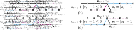
Figure 11: Different possibilities of embedding $T^{\prime}$ for a node $u_{i}$ of type C. Nodes marked as black squares must be leafless as they are mapped to a joint vertex of $G$.

In the second case, the secondary tree $s$ contains exactly one degree-3 node, $v$, which is either the immediate neighbor of $u_{i}$, see Fig. 11(e–f), or there is a single leafless degree-2 node between $v$ and $u_{i}$, see Fig. 11(g–j). In both cases, $v$ is the root of two branches of $s$, which are in fact paths that we denote by $s_{1}$ and $s_{2}$. Let us assume that $|s_{1}|\leq|s_{2}|$ and that $v$ is a neighbor of $u_{i}$. If $o_{i-1}+|s_{2}|\leq 0$ then we can assign the longer path $s_{2}$ to the left part of the ladder (modulo the existence of a leafless node in case of equality) and set $o_{i}=|s_{1}|$ and, if there is a leafless node in $s_{1}$, $\beta_{i}=1$ (Fig. 11(e)). Else if $o_{i-1}+|s_{1}|\leq 0$ we assign $s_{1}$ to the left (modulo the existence of a leafless node in case of equality) and set $o_{i}=|s_{2}|$ and, if $s_{2}$ has a leafless node, $\beta_{i}=1$ (Fig. 11(f)). If $o_{i-1}+|s_{1}|>0$ then $s$ cannot be embedded on the lower path of $G$ at all and we report that $T^{\prime}$ is no subgraph of a stegosaurus $G$.

If there is a node $w$ between $u_{i}$ and $v$, we need to map $w$ to a joint vertex of $G$. We have two options of arranging $s_{1}$ and $s_{2}$ on the left and right part of the ladder and two options of positioning $w$, see Fig. 11(g–j). Among these four combinations, we again pick the one that satisfies the constraints for the left side and minimizes the offset $o_{i}$ (if there is a tie and one of the paths contains a leafless node, we pick the option that yields $\beta_{i}=1$).

Type D. If $u_{i}$ is of type D we simply extend $\Pi$ and assign $u_{i}$ to be part of the upper path just as its predecessor $u_{i-1}$. The new offset $o_{i}$ is obtained by decreasing the previous offset $o_{i-1}$ by one, i.e., $o_{i}=o_{i-1}-1$. The existence of a leafless node on the ladder path is also simply inherited, i.e., we set $\beta_{i}=\beta_{i-1}$.

Figure 12: Different possibilities of embedding $T^{\prime}$ for a node triple $u_{i-1},u_{i},u_{i+1}$ of type B. Nodes marked as black squares must be leafless as they are mapped to a joint vertex of $G$.

Type B. Triples of type B are a special case to consider. Let $u_{i-1},u_{i},u_{i+1}$ be the triple vertices, and let $s_{1}$, $s_{2}$ be the secondary paths rooted in $u_{i-1}$, $u_{i+1}$, respectively. In this triple the leafless degree-two vertex $u_{i}$ can be mapped to a joint vertex of $G$, which allows a local backward flip of the secondary paths $s_{1}$ and $s_{2}$. Figure 12(a) shows the only configuration of the triple, in which path $s_{2}$ is mapped to the left part of the ladder and path $s_{1}$ to the right part, despite $u_{i+1}$ being two positions right of $u_{i-1}$ in $\Pi$. This is possible if $o_{i-2}+|s_{2}|\leq 0$ (modulo the existence of a leafless node in case of equality) and yields a new offset of $o_{i+1}=|s_{1}|-1$ and flag $\beta_{i+1}=1$ if $s_{1}$ contains a leafless node. Moreover, this is the only case, in which $\Pi$ changes from the upper path of $G$ to the lower path (or vice versa). If, on the other hand, we do not apply the backward flip, then the embedding options of the type-B triple are the same as treating it as a sequence of the type-C node $u_{i-1}$, the type-D node $u_{i}$, and the type-C node $u_{i+1}$. As a consequence, all of them embed the secondary path $s_{1}$ left of $s_{2}$. For completeness, Fig. 12(b–i) illustrate all relevant combinations. The details have been already discussed for types C and D.

We finally reintroduce the degree-one vertices that we removed when going from $T$ to $T^{\prime}$. We claim that this is always possible and that the leaves of $T$ can always be viewed as stumps or joints of a stegosaurus $G$. So far we mapped each vertex of $T^{\prime}$ as either a ladder or a joint vertex, and in the latter case such a vertex has no leaves in $T$. Moreover, we know for each ladder vertex whether it belongs to the upper path or to the lower path of a ladder. With this mapping of vertices to ladders, our goal is to reinsert the missing edges and vertices that form a stegosaurus $G$ containing $T$ as a (not necessarily spanning) subgraph. In particular, since $T^{\prime}$ does not contain cycles, all edges that connect a vertex on the upper path of a ladder to the corresponding vertex in the lower path are missing. Moreover, there is also a non-empty sub-path missing in either the upper path or the lower path of each ladder, say the upper path, which leaves some freedom in the reconstruction of $G$. We will exploit this freedom for the reinsertion of the leaves of $T$. Consider a ladder $L$ underlying a snake $N$ of $G$ and consider the sub-path $S$ of $L$ that is not in $T^{\prime}$. Assume first that $S$ contains at least one vertex, then this vertex does not belong to $T$, as we assume the leaves of $T$ be stumps or joints. We reinsert $S$ and we draw the edges that connect opposite ladder vertices of $L$ so to fully reconstruct $L$. See Fig. 13(a) for an illustration where the edges not in $T$ are dashed and the vertex not in $T$ is larger. In order to reinsert the leaves of $T$ that are adjacent to vertices of $L$, consider first the two mergeable vertices of $N$. Their leaves can be reinserted as stumps. Consider now the leftmost and the rightmost cells of $L$, i.e., those that contain the two mergeable vertices. If they coincide, then there is only one vertex of $L$ whose leaves need to be reinserted, and we can reinsert them as joint vertices that belong to this cell. If they don’t coincide, then we assign the leaves as shown in Fig. 13(b), where the leaves are solid disks (the figure shows the case in which the two mergeable vertices of $N$ are on the same path of $L$, the case in which are on opposite paths is similar).

(a)  

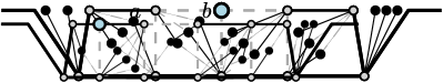
(b)  

(c)  

(d)  

Figure 13: Illustration for the leaves reinsertion step.

Suppose now that $S$ contains just one edge, call it $(a,b)$. Add $(a,b)$ and draw the edges that connect opposite ladder vertices as to fully reconstruct $L$, see Fig. 13(c). We call the cell of $L$ containing $(a,b)$ central. The previous greedy algorithm guarantees that all the leaves of $T$ adjacent to vertices that belong to the cells to left or to the right of the central one can be reinserted without using the central cell. This is due to the fact that in one of the two corresponding secondary paths there is a leafless node and hence the leaves can be reinserted as in the previous case (see Fig. 13(d) where the leafless node is large). Thus we can use the freedom given by the central cell to assign the leaves of the other secondary path, as shown in Fig. 13(d) where the leafless node is on the left path and the right path uses the central cell.

The above algorithm works in linear time: It first constructs $T^{\prime}$ from $T$ by removing $O(n)$ leaves; it then traverses $\Pi$ and makes a constant number of operations for each node of $\Pi$; it finally reinserts the removed leaves by reconstructing a stegosaurus $G$ that contains $T$ and has size $O(n)$. ∎

6 Summary and future directions

We studied layered drawings of fan-planar graphs. Motivated by the algorithm by Dujmović et al. [5], and using it as a subroutine, we gave an algorithm that tests the existence of a fan-plane proper ${h}$-layer drawing and is fixed-parameter tractable in $h$. (Variation can handle fan-plane short or 1-plane unconstrained drawings.) For the situation where the embedding of the graph is not fixed, we studied the existence of fan-planar proper ${2}$-layer drawings for trees. Along the way, we also bounded the pathwidth of graphs that have a fan-planar (short or proper) ${h}$-layer drawing, and argued that such graphs have a bar-1-visibility representation. Many open problems remain:

• Are there FPT algorithms to test whether a graph has a fan-planar ${h}$-layer drawing for $h>2$, presuming we can change the embedding? This problem was non-trivial even for trees and $h=2$ and proper drawings.

• Our FPT algorithm for 1-plane unconstrained ${h}$-layer drawing permits bends on the long edges. Is there an algorithm that tests for the existence of 1-plane straight-line ${h}$-layer drawing? We could easily test for a 1-plane $y$-monotone ${h}$-layer drawing, but in contrast to planar drawings, not all such drawings can be “stretched” to make edges straight-line.

• Our FPT algorithm for fan-plane drawings only worked for proper or short drawings. Is there an FPT algorithm if long edges are allowed?

• Likewise, our pathwidth-bounds work only for proper or short ${h}$-layer drawings. Does every graph with an fan-planar unrestricted ${h}$-layer drawings have pathwidth $O(h)$? Does it have a bar-1-visibility representation? Note that fan-planar graphs are not closed under subdividing edges, so we cannot simply replace long edges by paths.

• The dynamic programming algorithm by Dujmović et al. [5] is quite involved, and in particular, does not appeal to Courcelle’s theorem that states that any problem expressible in monadic second-order logic is solvable in polynomial time on graphs of bounded pathwidth [3]. This raises the natural question: Can we express whether a graph has a ${k}$-layer drawing (perhaps under some restrictions such as proper or fan-planar) in monadic second-order logic?

Last but not least, what do we know about layered drawings of $k$-planar graphs for $k>1$? Note that these are not necessarily fan-planar.

References

- [1] T. Biedl. Height-preserving transformations of planar graph drawings. In C. Duncan and A. Symvonis, editors, Graph Drawing (GD’14), volume 8871 of LNCS, pages 380–391. Springer, 2014.
- [2] C. Binucci, M. Chimani, W. Didimo, M. Gronemann, K. Klein, J. Kratochvíl, F. Montecchiani, and I. G. Tollis. Algorithms and characterizations for 2-layer fan-planarity: From caterpillar to stegosaurus. J. Graph Algorithms Appl., 21(1):81–102, 2017.
- [3] B. Courcelle. The monadic second-order logic of graphs. I. Recognizable sets of finite graphs. Inf. Comput., 85(1):12–75, 1990.
- [4] W. Didimo, G. Liotta, and F. Montecchiani. A survey on graph drawing beyond planarity. ACM Comput. Surv., 52(1):4:1–4:37, 2019.
- [5] V. Dujmovic, M. Fellows, M. Kitching, G. Liotta, C. McCartin, N. Nishimura, P. Ragde, F. Rosamond, S. Whitesides, and D. Wood. On the parameterized complexity of layered graph drawing. Algorithmica, 52:267–292, 2008.
- [6] S. Felsner, G. Liotta, and S. Wismath. Straight-line drawings on restricted integer grids in two and three dimensions. J. Graph Alg. Appl, 7(4):335–362, 2003.
- [7] L. Heath and A. Rosenberg. Laying out graphs using queues. SIAM J. Comput., 21(5):927–958, 1992.
- [8] M. Kaufmann and T. Ueckerdt. The density of fan-planar graphs. CoRR, abs/1403.6184, 2014.
- [9] S. G. Kobourov, G. Liotta, and F. Montecchiani. An annotated bibliography on 1-planarity. Computer Science Review, 25:49–67, 2017.
- [10] M. Schaefer. Crossing Numbers of Graphs. CRC Press, 2018.
- [11] M. Suderman. Pathwidth and layered drawings of trees. Intl. J. Comp. Geom. Appl., 14(3):203–225, 2004.