Optimal Signal-Adaptive Trading with Temporary and Transient Price Impact

Abstract

We study optimal liquidation in the presence of linear temporary and transient price impact along with taking into account a general price predicting finite-variation signal. We formulate this problem as minimization of a cost-risk functional over a class of absolutely continuous and signal-adaptive strategies. The stochastic control problem is solved by following a probabilistic and convex analytic approach. We show that the optimal trading strategy is given by a system of four coupled forward-backward SDEs, which can be solved explicitly. Our results reveal how the induced transient price distortion provides together with the predictive signal an additional predictor about future price changes. As a consequence, the optimal signal-adaptive trading rate trades off exploiting the predictive signal against incurring the transient displacement of the execution price from its unaffected level. This answers an open question from Lehalle and Neuman [29] as we show how to derive the unique optimal signal-adaptive liquidation strategy when price impact is not only temporary but also transient.

Mathematics Subject Classification (2010):

93E20, 60H30, 91G80

JEL Classification:

C02, C61, G11

Keywords:

optimal portfolio liquidation, price impact, optimal stochastic control, predictive signals

1 Introduction

The trading costs of executing large orders on an electronic trading platform often arise from the notion of price impact. Price impact refers to the empirical fact that the execution of a large order affects the risky asset’s price in an adverse manner leading to less favorable prices. This typically induces additional execution costs for the trader. As a result, a trader who wishes to minimize her trading costs due to price impact has to split her order into a sequence of smaller orders which are executed over a finite time horizon. At the same time, the trader also has an incentive to execute these split orders rapidly because she does not want to carry the risk of an adverse price move far away from her initial decision price. This trade-off between price impact and market risk is usually translated into a stochastic optimal control problem where the trader aims to minimize a risk-cost functional over a suitable class of execution strategies. The corresponding optimal order execution problem has been extensively studied in the literature and continues to be of ongoing interest in research and practice. We refer to the monographs [13], [26], [30], as well as the survey papers [21] and [23] for a thorough account for the developed price impact models.

In practice, apart from focusing on the aforementioned trade-off between price impact and market risk, many traders and trading algorithms also strive for using short term price predictors in their dynamic order execution schedules. Most of such documented predictors relate to orderbook dynamics as discussed in [28, 29, 31, 34]. An example of such price predicting indicator is the order book imbalance signal, measuring the imbalance of the current liquidity in the limit order book; see, e.g., Section 4 of [29] and references therein. Another signal which was studied in the literature in the context of optimal order execution is the order flow imbalance; we refer to [12, 34, 7, 8] and references therein. More examples of trading signals being used in practice can be found in a presentation by Almgren [2].

Consequently, one of the main challenges in the area of optimal trading with price impact deals with the question of how to incorporate short term predictive signals into a stochastic control framework of cost-risk minimization. Among the first to address this issue were Cartea and Jaimungal [12] who showed how to account for a Markovian signal in an optimal execution problem in the presence of linear temporary and permanent price impact of Almgren and Chriss [3] type. Their framework was then further generalized by Lehalle and Neuman [29], Section 3, and by Belak et al. [9] who also allowed for non-Markovian finite variation signals; see also Casgrain and Jaimungal [14] for incorporating latent factors into the modeling framework of [12]. Subsequently, a Markovian signal and transient price impact for a general class of impact decay kernels as proposed by Gatheral et al. [22] were first confronted in Lehalle and Neuman [29], Section 2. In contrast to purely temporary price impact, transient impact on execution prices persists and decays over a certain period of time after each trade. As a consequence, optimal trading strategies in the presence of purely transient price impact are typically singular. Indeed, they tend to trigger a displacement of the market price from its unaffected level via an instantaneous non-infinitesimal block trade in order to systematically exploit the successively decaying impact at a finite trading rate as, e.g., illustrated by the explicit results in Obizhaeva and Wang [33]. Mathematically, this renders the analysis of optimal signal-adaptive trading strategies with transient price impact much more intricate. A remedy, employed by the authors in [29], consists of confining to deterministic (or static) strategies which only use information of the predictive signal at initial time. The important question about existence and characterization of an optimal signal-adaptive strategy with transient price impact was left open. In fact, in Bellani et al. [10] it was shown that a strategy which is updated by information from the signal several times during the liquidation period can significantly improve the trading performance compared to an optimal static strategy. A partial solution to this problem was proposed by Lorenz and Schied [32], who considered an execution model with exponentially decaying transient price impact, but without including a risk-aversion term in the cost functional. Under the assumption that the signal is absolutely continuous with a square integrable derivative the optimal adapted strategy was derived. Moreover, since only transient price impact was considered in the model of [32], the optimal strategy is singular and involves block trades. We will show in this paper that once assuming that the price impact is both transient and temporary, we can omit these regularity assumptions on the signal and obtain absolutely continuous optimal trading strategies. In addition, we show that the influence of the risk-aversion term in the cost functional changes drastically the qualitative behaviour of the optimal trading speed.

The main result in the present paper gives an answer to the open question from [29]. Specifically, in order to optimize trading costs in the presence of exponentially decaying transient price impact as proposed by Obizhaeva and Wang [33] over a sensible set of strategies adapted to the signal’s filtration, we adopt the price impact model from Gârleanu and Pedersen [20]. We incorporate into the trader’s cost-risk functional besides a linear transient price impact component à la Obizhaeva-Wang also a linear temporary price impact component of Almgren-Chriss type. This unifying framework with temporary and transient price impact quadratically smoothens the problem and rules out singular optimizers by naturally constraining strategies to be absolutely continuous. Moreover, it turns out that the probabilistic and convex analytic calculus of variations approach from Bank et al. [6] can be brought to bear to compute explicitly optimal signal-adaptive strategies, also in a setup which allows for more general non-Markovian signals compared to [29, 20, 32]. Following the analysis in [20], the crucial idea is to introduce the displacement of the execution price from its unaffected level due to transient price impact as an additional state variable. Then, similar to [6] the optimal control is characterized by a system of coupled linear forward-backward stochastic differential equations (FBSDEs) which is augmented by a linear forward equation for the transient price distortion as well as an associated adjoint linear backward SDE. This linear system can be decoupled and solved in closed form. Its solution provides an explicit description of the optimal trading rate. It turns out that the transient price distortion provides together with the predictive signal an additional predictor for future price changes. Accordingly, the optimal trading rate compensates the exploitation of the predictive signal with the incurred transient price impact.

Our results in this paper improve the results of Cartea and Jaimungal [12] and Belak et al. [9] as we additionally allow for transient price impact. In our setting the optimal strategy depends on the entire trading trajectory, unlike the Markovian optimal strategies in the strictly instantaneous price impact case. Our main results also generalize the results of Graewe and Horst [24], Chen et al. [15], Gatheral et al. [22], Schied et al. [36] and Strehle [37], who study optimal liquidation with both temporary and transient price impact, but without a predictive price signal. This class of problems typically leads to deterministic optimal strategies. However, signal-adaptive optimal execution schedules have major practical significance, as described above. Finally, our paper is also related to a very recent work by Forde et al. [18], where an optimal liquidation problem with power-law transient price impact and Gaussian signals is studied.

Our findings also relate to a class of optimal portfolio choice problems: see, e.g., Gârleanu and Pedersen [20], and Ekren and Muhle-Karbe [17] for a setup of a portfolio optimizing agent that tries to exploit partially predictable returns while facing linear temporary and transient price impact. Unlike in our optimal execution framework, the trading time horizon in these optimal investment problems is infinite, and the agent perpetually invests simultaneously in a few assets having their own signals. The ansatz for the value function is typically a second order polynomial, which makes the derivation of the latter as well as the corresponding optimal strategy much easier than in the parabolic case where the time horizon is finite. Moreover, both [20] and [17] study a Markovian setup via dynamic programming techniques: [20] describes the optimal trading rate where the predictable returns are driven by a jump-diffusion process, an assumption which is not needed in the present paper since we allow a general signal in our model; [17] studies the case where the signal is a Markovian diffusion process which interacts with the asset prices through their drift vector and covariance matrix. They derive an asymptotic optimal trading strategy in the case when both temporary and transient price impact tend to zero. In contrast, we derive the optimal strategy not under the restriction of vanishing price impact.

The rest of the paper is organized as follows. In Section 2 we introduce our optimal execution problem with temporary and transient price impact and predictable finite-variation signal. Our main result, an explicit solution to our optimal stochastic control problem, is presented in Section 3. Section 4 contains some illustrations. The technical proofs are deferred to Section 5.

2 Model setup and problem formulation

Motivated by Lehalle and Neuman [29] we introduce in the following a variant of the optimal signal-adaptive trading problem with transient price impact which was studied in Section 2 therein.

Let $T>0$ denote a finite deterministic time horizon and fix a filtered probability space $(\Omega,\mathcal{F},(\mathcal{F}_{t})_{0\leq t\leq T},\mathbb{P})$ satisfying the usual conditions of right continuity and completeness. The set $\mathcal{H}^{2}$ represents the class of all (special) semimartingales $P=(P_{t})_{0\leq t\leq T}$ whose canonical decomposition $P=\bar{M}+A$ into a (local) martingale $\bar{M}=(\bar{M}_{t})_{0\leq t\leq T}$ and a predictable finite-variation process $A=(A_{t})_{0\leq t\leq T}$ satisfies

$$E\left[\langle\bar{M}\rangle_{T}\right]+E\left[\left(\int_{0}^{T}|dA_{s}|\right)^{2}\right]<\infty.$$ (2.1)

We consider a trader with an initial position of $x>0$ shares in a risky asset. The number of shares the trader holds at time $t\in[0,T]$ is prescribed as

$$X^{u}_{t}\triangleq x-\int_{0}^{t}u_{s}ds$$ (2.2)

where $(u_{s})_{s\in[0,T]}$ denotes her selling rate which she chooses from a set of strategies

$$\mathcal{A}\triangleq\left\{u\,:\,u\textrm{ progressively measurable s.t. }\mathbb{E}\left[\int_{0}^{T}u_{s}^{2}ds\right]<\infty\right\}.$$ (2.3)

We assume that the trader’s trading activity causes price impact on the risky asset’s execution price in the sense that her orders are filled at prices

$$S_{t}\triangleq P_{t}-\lambda u_{t}-\kappa Y^{u}_{t}\qquad(0\leq t\leq T),$$ (2.4)

where $P$ denotes some unaffected price process in $\mathcal{H}^{2}$ and

$$Y^{u}_{t}\triangleq e^{-\rho t}y+\gamma\int_{0}^{t}e^{-\rho(t-s)}u_{s}ds\qquad(0\leq t\leq T)$$ (2.5)

with some $y>0$. Specifically, motivated by Gârleanu and Pedersen [20] the trader’s trading not only instantaneously affects the execution price in (2.4) in an adverse manner through linear temporary price impact $\lambda>0$ à la Almgren and Chriss [3]; it also induces a longer lasting price distortion $Y^{u}$ because of linear transient price impact $\kappa>0$ and $\gamma>0$ as proposed by Obizhaeva and Wang [33]. We assume that the transient price impact, which starts from an initial value $y>0$, persists and decays only gradually over time at some exponential resilience rate $\rho>0$. Also note that the unaffected price process $P\in\mathcal{H}^{2}$ includes a general signal process $A$ which is observed by the trader.

We now suppose that the trader’s optimal trading objective is to unwind her initial position $x>0$ in the presence of temporary and transient price impact, along with taking into account the asset’s general price signal $A$, through maximizing the performance functional

$$J(u)\triangleq\mathbb{E}\Bigg{[}\int_{0}^{T}(P_{t}-\kappa Y^{u}_{t})u_{t}dt-\lambda\int_{0}^{T}u^{2}_{t}dt+X_{T}^{u}P_{T}\Bigg{.}$$ (2.6)

$$\Bigg{.}\hskip 60.0pt-\phi\int_{0}^{T}(X_{t}^{u})^{2}dt-\varrho(X_{T}^{u})^{2}\Bigg{]}$$

via her selling rate $u\in\mathcal{A}$. The interpretation is as follows (cf. also Remark 2.1.1.) below). The first three terms in (2.6) represent the trader’s terminal wealth; that is, her final cash position including the accrued trading costs which are induced by temporary and transient price impact as prescribed in (2.4), as well as her remaining final risky asset position’s book value. The fourth and fifth terms in (2.6) implement a penalty $\phi>0$ and $\varrho>0$ on her running and terminal inventory, respectively. Also observe that $J(u)<\infty$ for any admissible strategy $u\in\mathcal{A}$.

Our main goal in this paper is to solve the corresponding optimal stochastic control problem

$$J(u)\rightarrow\max_{u\in\mathcal{A}}.$$ (2.7)

Remark 2.1.

1. In case of purely temporary price impact, i.e., $\kappa=0$, the performance functional in (2.6) and the associated optimization problem in (2.7) is quite standard in the literature on optimal trading and execution problems. It was first introduced by [1, 19] and then subsequently studied, e.g., in [35, 4, 25, 12, 29, 9].

2. Our problem formulation in (2.6) with temporary and transient price impact is very similar to the framework introduced in Gârleanu and Pedersen [20] which was then further analyzed by Ekren and Muhle-Karbe [17]. In contrast to their setup, we focus on a finite time horizon $T<\infty$. We also allow for more general price signal processes $A$ and not only a linear factor process as in [20] or a Markovian diffusion-type process as in [17]. Moreover, we obtain an explicit solution to our optimization problem in (2.7), akin to the results established by [20] in their simpler framework, and do not necessitate an asymptotic analysis as carried out in [17].

3. As mentioned at the beginning of this section our framework presented above also aims at following up on the optimal signal-adaptive trading problem in the presence of transient price impact which was studied in Section 2 of [29]. Therein, the authors confine themselves to analyze only deterministic optimal strategies. Indeed, optimal strategies in a purely transient price impact setup are typically singular (cf., e.g., [33, 22, 32, 5]) which renders the analysis for signal-adaptive strategies mathematically much more intricate. As a remedy, we adopt the approach from [20]. We incorporate into the cost functional in (2.6) in addition to the transient price impact also a temporary impact component via $\lambda>0$ which rules out singular optimizers. This quadratically smoothens the problem and very naturally constrains strategies to be absolutely continuous. Also note that we do not require the signal processes $A$ to be an integrated Markov process as in [29].

4. For $A\equiv 0$, that is, without price signal process, but with terminal liquidation constraint $X^{u}_{T}=0$ $\mathbb{P}$-a.s. the above optimization problem in (2.7) was studied in Graewe and Horst [24] allowing for stochastic resilience and temporary price impact processes $(\rho_{t})_{0\leq t\leq T}$ and $(\lambda_{t})_{0\leq t\leq T}$, respectively. For the corresponding explicitly available deterministic solution in the case of constant coefficients and $\phi=0$ we refer to [15]. As, e.g, in [12, 29, 9], we do not incorporate a terminal state constraint in our optimization problem in (2.7). Note, however, that the terminal penalty $\varrho>0$ on the remaining risky asset position allows to virtually enforce a liquidation constraint by choosing a large value for $\varrho$ (see also the illustrations in Section 4 below).

3 Main result

Our main result is an explicit description of the optimal strategy for problem (2.7). To state our result it is convenient to introduce for

$$L\triangleq\begin{pmatrix}0&0&-1&0\\ 0&-\rho&\gamma&0\\ -\phi/\lambda&\kappa\rho/(2\lambda)&0&\rho/(2\lambda)\\ 0&0&\kappa\gamma&\rho\end{pmatrix}\in\mathbb{R}^{4\times 4}$$ (3.1)

the functions $S(t)=(S_{ij}(t))_{1\leq i,j\leq 4}$ given by the matrix exponential

$$S(t)\triangleq e^{Lt}\qquad(t\geq 0).$$ (3.2)

We further define $G(t)=(G_{i}(t))_{1\leq i\leq 4}$ as

$$G(t)\triangleq\left(\varrho/\lambda,-\kappa/(2\lambda),-1,0\right)S(t)\qquad(t\geq 0)$$ (3.3)

and let

$$v_{0}(t)\triangleq\left(1-\frac{G_{4}(t)}{G_{3}(t)}\frac{S_{4,3}(t)}{S_{4,4}(t)}\right)^{-1}, v_{1}(t)\triangleq \;\frac{G_{4}(t)}{G_{3}(t)}\frac{S_{4,1}(t)}{S_{4,4}(t)}-\frac{G_{1}(t)}{G_{3}(t)},$$ (3.4)

$$v_{2}(t)\triangleq\frac{G_{4}(t)}{G_{3}(t)}\frac{S_{4,2}(t)}{S_{4,4}(t)}-\frac{G_{2}(t)}{G_{3}(t)}, v_{3}(t)\triangleq \;\frac{G_{4}(t)}{G_{3}(t)}$$

for all $t\in[0,\infty)$. The functions $(S_{4,j}(t))_{1\leq j\leq 4}$ and $(G_{i}(t))_{1\leq i\leq 4}$ can be computed explicitly and are given in (5.25)-(5.28) and (5.29)-(5.32), respectively, in Section 5.2 below. Lemma 5.5 therein also shows that $v_{1}(\cdot),v_{2}(\cdot),v_{3}(\cdot)$ are well-defined. In addition, we make following assumption below (see also Remark 3.4.1.).

Assumption 3.1.

We assume that the set of parameters $\xi\triangleq(\lambda,\gamma,\kappa,\rho,\varrho,\phi,T)\in\mathds{R}^{7}_{+}$ are chosen such that

$$G_{3}(T-t)S_{4,4}(T-t)\neq G_{4}(T-t)S_{4,3}(T-t)\qquad(0\leq t\leq T).$$ (3.5)

Finally, let $\mathbb{E}_{t}$ denote the expectation conditioned on $\mathcal{F}_{t}$ for all $t\in[0,T]$. We are now ready to state our main theorem.

Theorem 3.2.

Under Assumption 3.1, there exists a unique optimal strategy $\hat{u}\in\mathcal{A}$ to problem (2.7). It is given in linear feedback form via

$$\hat{u}_{t}= \;v_{0}(T-t)\Bigg{(}v_{1}(T-t)X^{\hat{u}}_{t}+v_{2}(T-t)Y^{\hat{u}}_{t}\Bigg{.}$$ (3.6)

$$+\frac{1}{2\lambda}\Bigg{.}\bigg{(}v_{3}(T-t)\mathbb{E}_{t}\left[\int_{t}^{T}\frac{S_{4,3}(T-s)}{S_{4,4}(T-t)}dA_{s}\right]-\mathbb{E}_{t}\left[\int_{t}^{T}\frac{G_{3}(T-s)}{G_{3}(T-t)}dA_{s}\right]\bigg{)}\Bigg{)}$$

for all $t\in(0,T)$.

The proof of Theorem 3.2 is deferred to Section 5.1. We observe that the optimal trading rate $\hat{u}$ in (3.6) is affine-linear in both the current inventory $X^{\hat{u}}$ as well as the current price distortion $Y^{\hat{u}}$. The affine part comes from the general predictive signal $A$. In particular, it turns out that the transient price displacement from the unaffected level serves as an additional predictor for future price changes. As a consequence, the optimal trading rate trades off exploiting the predictive signal $A$ against incurring transient price distortion $Y^{\hat{u}}$. These findings generalize the observations made in Gârleanu and Pedersen [20] for optimal portfolio choice problems with infinite horizon in a Markovian setup. Put differently, the optimal stock holdings $X^{\hat{u}}$ prescribed by the optimal selling rate $\hat{u}$ in (3.6) together with the optimally controlled price distortion $Y^{\hat{u}}$ in (2.5) solve a two-dimensional system of coupled linear (random) ordinary differential equations. Its solution can be computed numerically via the associated fundamental solution. Specifically, introducing the process

$$\hat{\zeta}_{t}\triangleq\frac{v_{0}(T-t)}{2\lambda}\bigg{(}v_{3}(T-t)\mathbb{E}_{t}\left[\int_{t}^{T}\frac{S_{4,3}(T-s)}{S_{4,4}(T-t)}dA_{s}\right]-\mathbb{E}_{t}\left[\int_{t}^{T}\frac{G_{3}(T-s)}{G_{3}(T-t)}dA_{s}\right]\bigg{)}$$ (3.7)

as well as the matrix-valued function

$$B(t)\triangleq\begin{pmatrix}-v_{0}(T-t)v_{1}(T-t)&-v_{0}(T-t)v_{2}(T-t)\\ \gamma v_{0}(T-t)v_{1}(T-t)&\gamma v_{0}(T-t)v_{2}(T-t)-\rho\end{pmatrix}$$ (3.8)

for all $t\in[0,T]$, we obtain following

Corollary 3.3.

Under Assumption 3.1 let $\Phi(t)\in\mathbb{R}^{2\times 2}$ be the unique nonsingular fundamental solution to the matrix differential equation

$$\Phi(0)=I,\quad\dot{\Phi}(t)=B(t)\Phi(t)\quad(0\leq t\leq T)$$ (3.9)

with identity matrix $I\in\mathbb{R}^{2\times 2}$ and $B$ as defined in (3.8). Then the optimal stock holdings $X^{\hat{u}}$ and the corresponding optimally controlled price distortion $Y^{\hat{u}}$ of the optimal strategy $\hat{u}$ from Theorem 3.2 are given by

$$\begin{pmatrix}X^{\hat{u}}_{t}\\ Y^{\hat{u}}_{t}\end{pmatrix}=\Phi(t)\left(\begin{pmatrix}x\\ y\end{pmatrix}+\int_{0}^{t}\hat{\zeta}_{s}\,\Phi^{-1}(s)\,b\,ds\right),$$ (3.10)

where $b\triangleq(-1,\gamma)^{\top}\in\mathbb{R}^{2}$.

Again, the proof of Corollary 3.3 can be found in Section 5.1.

Remark 3.4.

1. Assumption 3.1 merely ensures that $v_{0}(\cdot)$ in (3.4) is well-defined. In fact, showing that (3.5) holds for any values of parameters $\xi\in\mathds{R}^{7}_{+}$ seems intractable. However, given a set of parameters $\xi$ and verifying that (3.5) is satisfied is an easy task by using the explicit formulas for $S_{4,3},S_{4,4},G_{3},G_{4}$ in (5.27), (5.28), (5.31), (5.32). We numerically checked this for all $\xi\in[0,100]^{7}$, which includes all reasonable values of parameters.

2. The special case where $\kappa=0$ in the performance functional in (2.6), i.e., considering only temporary price impact, corresponds to Belak et al. [9], and Lehalle and Neuman [29], Section 3. One can check with the explicit expressions from Section 5.2 that our result in Theorem 3.2 retrieves the optimal solution from [9], Theorem 3.1, as well as, in a Markovian setting, from [29], Proposition 3.2, in the limiting case when $\kappa$ tends to zero.

3. Note that our optimal strategy in Theorem 3.2 is adapted to the underlying filtration $(\mathcal{F}_{t})_{0\leq t\leq T}$ and hence steadily updates its information about the price signal process $A$. This is in stark contrast to the signal-adaptive optimal trading framework with transient price impact studied in Lehalle and Neuman [29], Section 2, where strategies are confined to be static (i.e., deterministic), taking only the information of the price signal at initial time 0 into account.

4 Illustration

Similar to Lehalle and Neuman [29] we will illustrate in this section our main result in the special case where the signal process $A$ is given by

$$A_{t}=\int_{0}^{t}I_{s}ds\qquad(t\geq 0)$$ (4.1)

with $I=(I_{t})_{t\geq 0}$ following an autonomous Ornstein-Uhlenbeck process with dynamics

$$I_{0} =\iota,\quad dI_{t}=-\beta I_{t}\,dt+\sigma\,dW_{t}\qquad(t\geq 0).$$ (4.2)

Here, $W=(W_{t})_{t\geq 0}$ denotes a standard Brownian motion which is defined on our underlying filtered probability space and $\beta,\sigma>0$ are some constants. Having at hand our general result from Theorem 3.2 we immediately obtain following optimal trading strategy in this case.

Corollary 4.1.

Assume that the signal process $A$ is given by (4.1). Then the unique optimal trading rate $\hat{u}\in\mathcal{A}$ from Theorem 3.2 simplifies to

$$\hat{u}_{t}= \;v_{0}(T-t)\Bigg{(}v_{1}(T-t)X^{\hat{u}}_{t}+v_{2}(T-t)Y^{\hat{u}}_{t}\Bigg{.}$$ (4.3)

$$+\frac{I_{t}}{2\lambda}\Bigg{.}\bigg{(}v_{3}(T-t)\int_{t}^{T}e^{-\beta(s-t)}\frac{S_{4,3}(T-s)}{S_{4,4}(T-t)}ds-\int_{t}^{T}e^{-\beta(s-t)}\frac{G_{3}(T-s)}{G_{3}(T-t)}ds\bigg{)}\Bigg{)}.$$

for all $t\in(0,T)$.

Remark 4.2.

Observe that the optimal trading rate in (4.3) is signal-adaptive, i.e., adapted to the filtration generated by $I$, in contrast to the optimal solution presented in Section 2.3 of [29].

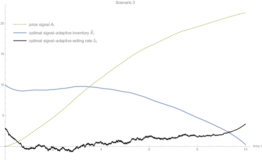
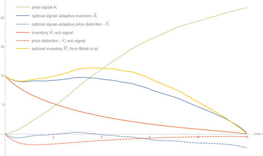
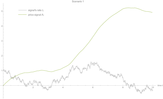
In Figures 1 to 4 we plot the signal-adaptive optimal liquidation inventory $\hat{X}\triangleq(X^{\hat{u}}_{t})_{0\leq t\leq T}$ with initial position $x=10$ along with the corresponding optimal selling rate $(\hat{u})_{0\leq t\leq T}$ and optimally controlled price distortion $\hat{Y}\triangleq(Y^{\hat{u}}_{t})_{0\leq t\leq T}$ with $y=0$ obtained from Corollary 4.1 (by using also Corollary 3.3) for three different realisations of the signal process $(A_{t})_{0\leq t\leq T}$ in (4.1). The trader’s planning horizon is $T=10$. As for the model parameters, we fix the values

$$\kappa=1,\quad\gamma=1,\quad\rho=1,\quad\lambda=0.5,\quad\phi=0.1,\quad\varrho=10,$$ (4.4)

as well as

$$\iota=1,\quad\beta=0.1,\quad\sigma=0.5,$$ (4.5)

similar to the parameters in [29] (cf. also the empirical analysis in Section 4.2 therein). As mentioned in Remark 3.4.1. above, one can easily check that Assumption 3.1 holds true with this set of parameter values. We also compare graphically our signal-adaptive optimal liquidation strategy $\hat{X}$ with (i) the inventory $\tilde{X}\triangleq(\tilde{X}_{t})_{0\leq t\leq T}$ and corresponding induced price distortion trajectory $\tilde{Y}\triangleq(\tilde{Y}_{t})_{0\leq t\leq T}$ which ignores the price signal, i.e., $I\equiv 0$ in (4.3); (ii) the optimal signal-adaptive inventory trajectory $\bar{X}\triangleq(\bar{X}_{t})_{0\leq t\leq T}$ for the purely temporary price impact case from Theorem 3.1 in [9]. Note that the former is simply the optimal strategy for the maximization problem in (2.7) where the trader presumes that the unaffected price process $P$ has no signal, and the latter corresponds to the optimal strategy where $\kappa=0$ in (2.6), i.e., the trader ignores transient price distortion.

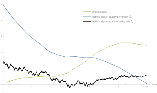
Figure 1: Upper panel: Realization of the signal rate $I_{t}$ (solid grey) and corresponding signal process $A_{t}$ (dashed green). Lower panel: Optimal signal-adaptive inventory (solid blue) and corresponding selling rate (solid black) for the same signal process (dashed green) as in the upper panel.

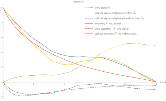
Figure 2: Comparison between the optimal signal-adaptive inventory (solid blue) and corresponding price distortion (dashed blue) with the optimal inventory (solid red) and corresponding price distortion (dashed red) ignoring the signal, as well as with the optimal signal-adaptive inventory with purely temporary price impact (solid yellow) for the same signal process (dashed green) as in Figure 1.

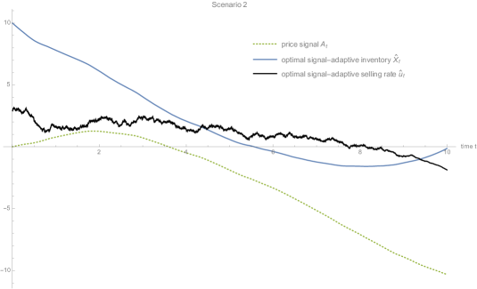
Figure 3: Upper panel: Similar to the lower panel of Figure 1, optimal signal-adaptive inventory (solid blue) and corresponding selling rate (solid black) for a strongly decreasing price signal process (dashed green). Lower panel: Similar to Figure 2, comparison of the different optimal inventory and corresponding price distortion trajectories for the same signal process (dashed green) as in the upper panel.

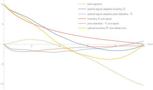
Figure 4: Upper panel: Similar to the upper panel of Figure 3, optimal signal-adaptive inventory (solid blue) and corresponding selling rate (solid black) for a strongly increasing price signal process (dashed green). Lower Panel: Similar to the lower panel of Figure 3, comparison of the different optimal inventory and corresponding price distortion trajectories.

Figure 1 on the upper panel shows a realization of the Ornstein-Uhlenbeck signal rate process $(I_{t})_{0\leq t\leq T}$ as in (4.2) in solid grey together with the resulting price signal process $(A_{t})_{0\leq t\leq T}$ from (4.1) in dashed green. On the lower panel, we illustrate the corresponding optimal signal-adaptive inventory $\hat{X}$ together with its selling rate $\hat{u}$. In Figure 2 we compare the optimal signal-adaptive inventory $\hat{X}$ and corresponding price distortion $\hat{Y}$ (depicted in solid and dashed blue, respectively) for the same price signal trajectory from Figure 1 with the optimal inventory $\tilde{X}$ and price distortion $\tilde{Y}$ ignoring the signal (depicted in solid and dashed red, respectively). We also plot in solid yellow the optimal inventory $\bar{X}$ for the purely temporary price impact case. Interestingly, one can observe some differences between the optimal strategies within the different frameworks. As expected, in contrast to the strictly decreasing inventory $\tilde{X}$ ignoring the price signal process, the signal-adaptive inventories $\hat{X}$ and $\bar{X}$ utilize their information about the upward trend of the latter and slow down the liquidation of the risky asset midway. Moreover, the inventory $\bar{X}$ taking into account only temporary price impact does so more aggressively which results in trading also in the opposite direction and buying some shares of the risky asset amid its liquidation schedule.

Figures 3 and 4 illustrates in similar fashion the optimal inventory, selling rate and price distortion trajectories for two extreme scenarios: A strongly decreasing price signal (Figure 3) and a strongly increasing price signal (Figure 4). Again, we observe that in a purely temporary price impact setup the trader tends to take more risks by trading more boldly in the opposite direction to her selling intentions in order to profit from the perceived information about the price signal’s tendencies. In fact, recall that the feedback form of the optimal selling rate $\hat{u}$ in (4.3) compensates for the induced price distortion $Y^{\hat{u}}$. It is therefore sensible to expect that this results in the observed deceleration of the overall turnover rate as shown by the graphs in Figures 1 to 4.

5 Proofs

5.1 Proof of Theorem 3.2

In fact, the probabilistic and convex analytic calculus of variations approach from Bank et al. [6] can be brought to bear to prove our main Theorem 3.2. Indeed, note that for any $u\in\mathcal{A}$ the map $u\mapsto J(u)$ in (2.6) is strictly concave. Therefore, it admits a unique maximizer characterized by the critical point at which the Gâteaux derivative

$$\langle J^{\prime}(u),\alpha\rangle\triangleq\lim_{\varepsilon\rightarrow 0}\frac{J(u+\varepsilon\alpha)-J(u)}{\varepsilon}$$ (5.1)

of the functional $J$ vanishes for any direction $\alpha=(\alpha_{t})_{0\leq t\leq T}\in\mathcal{A}$; see, e.g., [16]. The Gâteaux derivative in (5.1) can be readily computed.

Lemma 5.1.

For $u\in\mathcal{A}$ we have

$$\langle J^{\prime}(u),\alpha\rangle =\mathbb{E}\Bigg{[}\int_{0}^{T}\alpha_{s}\left(P_{s}-\kappa Y^{u}_{s}-\kappa\int_{s}^{T}e^{-\rho(t-s)}\gamma u_{t}dt-2\lambda u_{s}\right.\Bigg{.}$$ (5.2)

$$\hskip 75.0pt\Bigg{.}\Bigg{.}+2\phi\int_{s}^{T}X^{u}_{t}dt+2\varrho X^{u}_{T}-P_{T}\Bigg{)}ds\Bigg{]}$$

for any $\alpha\in\mathcal{A}$.

Proof.

Let $\varepsilon>0$ and $u,\alpha\in\mathcal{A}$. Note that $X_{t}^{u+\varepsilon\alpha}=X_{t}^{u}-\varepsilon\int_{0}^{t}\alpha_{s}ds$ and $Y_{t}^{u+\varepsilon\alpha}=Y^{u}_{t}+\varepsilon\gamma\int_{0}^{t}e^{-\rho(t-s)}\alpha_{s}ds$ for all $t\in[0,T]$. Next, since

$$J(u+\varepsilon\alpha)-J(u)$$

$$=\varepsilon\;\mathbb{E}\Bigg{[}\int_{0}^{T}\left(P_{t}-\kappa Y^{u}_{t}\right)\alpha_{t}dt-\kappa\int_{0}^{T}u_{t}\left(\int_{0}^{t}e^{-\rho(t-s)}\gamma\alpha_{s}ds\right)dt$$

$$\hskip 40.0pt-2\lambda\int_{0}^{T}u_{t}\alpha_{t}dt+2\phi\int_{0}^{T}X^{u}_{t}\left(\int_{0}^{t}\alpha_{s}ds\right)dt$$

$$\hskip 40.0pt\Bigg{.}+2\varrho X_{T}^{u}\int_{0}^{T}\alpha_{s}ds-P_{T}\int_{0}^{T}\alpha_{s}ds\Bigg{]}$$

$$\quad+\varepsilon^{2}\;{\mathbb{E}}\Bigg{[}-\kappa\gamma\int_{0}^{T}\left(\int_{0}^{t}e^{-\rho(t-s)}\alpha_{s}ds\right)\alpha_{t}dt-\lambda\int_{0}^{T}\alpha_{t}^{2}dt\Bigg{.}$$

$$\hskip 55.0pt-\phi\int_{0}^{T}\left(\int_{0}^{t}\alpha_{s}ds\right)^{2}dt-\varrho\left(\int_{0}^{T}\alpha_{s}ds\right)^{2}\Bigg{]}$$

we obtain the desired result in (5.2) after applying Fubini’s theorem twice. Also observe that all terms are finite since $u,\alpha\in\mathcal{A}$. ∎

Given the explicit expression of the Gâteaux derivative in (5.2) we can now derive a first order optimality condition. It takes the form of a coupled system of linear forward backward stochastic differential equations.

Lemma 5.2.

A control $\hat{u}\in\mathcal{A}$ solves the optimization problem in (2.7) if and only if the processes $(X^{\hat{u}},Y^{\hat{u}},{\hat{u}},Z^{\hat{u}})$ satisfy following coupled linear forward backward SDE system

$$\left\{\begin{aligned} dX^{u}_{t}=&\,-u_{t}dt,\quad X^{u}_{0}=x\\ dY^{u}_{t}=&\,-\rho Y_{t}^{u}dt+\gamma u_{t}dt,\quad Y^{u}_{0}=y\\ du_{t}=&\,\frac{dP_{t}}{2\lambda}+\frac{\kappa\rho Y^{u}_{t}}{2\lambda}dt-\frac{\phi X^{u}_{t}}{\lambda}dt+\frac{\rho Z^{u}_{t}}{2\lambda}dt+dM_{t},\quad u_{T}=\frac{\varrho X^{u}_{T}}{\lambda}-\frac{\kappa Y^{u}_{T}}{2\lambda},\\ dZ^{u}_{t}=&\,\rho Z^{u}_{t}dt+\kappa\gamma u_{t}dt+dN_{t},\quad Z^{u}_{T}=0,\end{aligned}\right.$$ (5.3)

for two suitable square integrable martingales $M=(M_{t})_{0\leq t\leq T}$ and $N=(N_{t})_{0\leq t\leq T}$.

Remark 5.3.

The appearance of the auxiliary process $Z^{u}$ in the above FBSDE system (5.3) is very natural in our setup because of the two-dimensional controlled state variable $(X^{u},Y^{u})$ in (2.2) and (2.5). In fact, the two processes $u$ and $Z^{u}$ satisfying the BSDEs in (5.3) correspond to the two associated so-called adjoint processes which are arising in Pontryagin’s stochastic maximum principle; see, e.g., Carmona [11], Chapter 4.2.

Proof.

Since we are maximizing the strictly concave functional $u\mapsto J(u)$ over $\mathcal{A}$, a necessary and sufficient condition for the optimality of $\hat{u}\in\mathcal{A}$ with corresponding controlled state processes $X^{\hat{u}}$ and $Y^{\hat{u}}$ in (2.2) and (2.5), respectively, is given by

$$\langle J^{\prime}(\hat{u}),\alpha\rangle=0\;\text{for all }\alpha\in\mathcal{A};$$

cf., e.g., [16]. By Lemma 5.1 this condition is equivalent to

$$\mathbb{E}\Bigg{[}\int_{0}^{T}\alpha_{s}\bigg{(}P_{s}-\kappa Y^{\hat{u}}_{s}-\kappa\int_{s}^{T}e^{-\rho(t-s)}\gamma\hat{u}_{t}dt-2\lambda u_{s}$$ (5.4)

$$\hskip 58.0pt\Bigg{.}\Bigg{.}+2\phi\int_{s}^{T}X^{\hat{u}}_{t}dt+2\varrho X^{\hat{u}}_{T}-P_{T}\bigg{)}ds\Bigg{]}=0$$

for all $\alpha\in\mathcal{A}$. In the following we will argue that $\hat{u}\in\mathcal{A}$ with $(X^{\hat{u}},Y^{\hat{u}})$ satisfies the first order condition in (5.4) if and only if $(X^{\hat{u}},Y^{\hat{u}},{\hat{u}},Z^{\hat{u}})$ satisfy the FBSDE system in (5.3).

Necessity: Although necessity follows from the uniqueness of the optimal solution together with the sufficiency argument below, we give the complete proof here in order to shed light on the derivation of the FBSDE system in (5.3).

Assume that $\hat{u}\in\mathcal{A}$ maximizes $J$, i.e., the first order condition in (5.4) is satisfied. Then, by applying optional projection we also obtain that

$$\mathbb{E}\left[\int_{0}^{T}\alpha_{s}\left(P_{s}-\kappa Y^{\hat{u}}_{s}-\kappa\,\mathbb{E}_{s}\left[\int_{s}^{T}e^{-\rho(t-s)}\gamma\hat{u}_{t}dt\right]-2\lambda\hat{u}_{s}\right.\right.$$ (5.5)

$$\left.\left.\hskip 58.0pt+\,\mathbb{E}_{s}\left[2\phi\int_{s}^{T}X^{\hat{u}}_{t}dt+2\varrho X^{\hat{u}}_{T}-P_{T}\right]\right)ds\right]=0$$

for all $\alpha\in\mathcal{A}$. But this implies that

$$P_{s}-\kappa Y^{\hat{u}}_{s}-\kappa e^{\rho s}\mathbb{E}_{s}\left[\int_{s}^{T}e^{-\rho t}\gamma\hat{u}_{t}dt\right]-2\lambda\hat{u}_{s}+\mathbb{E}_{s}\left[2\phi\int_{s}^{T}X^{\hat{u}}_{t}dt+2\varrho X^{\hat{u}}_{T}-P_{T}\right]$$ (5.6)

$$=\,P_{s}-\kappa Y^{\hat{u}}_{s}-\kappa e^{\rho s}\left(\mathbb{E}_{s}\left[\int_{0}^{T}e^{-\rho t}\gamma\hat{u}_{t}dt\right]-\int_{0}^{s}e^{-\rho t}\gamma\hat{u}_{t}dt\right)-2\lambda\hat{u}_{s}$$

$$\hskip 12.0pt+\mathbb{E}_{s}\left[2\phi\int_{0}^{T}X^{\hat{u}}_{t}dt+2\varrho X^{\hat{u}}_{T}-P_{T}\right]-2\phi\int_{0}^{s}X^{\hat{u}}_{t}dt$$

$$=0\quad d\mathbb{P}\otimes ds\textrm{-a.e. on }\Omega\times[0,T].$$

Now, by introducing the square integrable martingales

$$\tilde{M}_{s}\triangleq\mathbb{E}_{s}\left[2\phi\int_{0}^{T}X^{\hat{u}}_{t}dt+2\varrho X^{\hat{u}}_{T}-P_{T}\right],\quad\tilde{N}_{s}\triangleq\mathbb{E}_{s}\left[\int_{0}^{T}e^{-\rho t}\gamma\hat{u}_{t}dt\right],$$ (5.7)

as well as the auxiliary square integrable process

$$Z^{\hat{u}}_{s}\triangleq\kappa e^{\rho s}\left(\int_{0}^{s}e^{-\rho t}\gamma\hat{u}_{t}dt-\tilde{N}_{s}\right)$$ (5.8)

for all $s\in[0,T]$ (note that $P_{T}\in L^{2}(\Omega,\mathcal{F}_{T},\mathbb{P})$ because of (2.1); and that $u\in L^{2}(\mathbb{P}\times[0,T])$ which also implies $X^{\hat{u}}_{T}\in L^{2}(\Omega,\mathcal{F}_{T},\mathbb{P})$), we can rewrite (5.6) as

$$P_{s}-\kappa Y^{\hat{u}}_{s}-\kappa e^{\rho s}\left(\tilde{N}_{s}-\int_{0}^{s}e^{-\rho t}\gamma\hat{u}_{t}dt\right)-2\lambda\hat{u}_{s}+\tilde{M}_{s}-2\phi\int_{0}^{s}X^{\hat{u}}_{t}dt$$ (5.9)

$$=P_{s}-\kappa Y^{\hat{u}}_{s}+Z^{\hat{u}}_{s}-2\lambda\hat{u}_{s}+\tilde{M}_{s}-2\phi\int_{0}^{s}X^{\hat{u}}_{t}dt$$

$$=0\quad d\mathbb{P}\otimes ds\textrm{-a.e. on }\Omega\times[0,T].$$

Note that $Z^{\hat{u}}$ in (5.8) satisfies the BSDE

$$dZ^{\hat{u}}_{t}=\rho Z^{\hat{u}}_{t}dt+\kappa\gamma\hat{u}_{t}dt-\kappa e^{\rho t}d\tilde{N}_{t},\qquad Z^{\hat{u}}_{T}=0.$$ (5.10)

Also observe that the controlled forward dynamics of $Y^{\hat{u}}$ in (2.5) satisfy

$$Y^{\hat{u}}_{0}=y,\quad dY^{\hat{u}}_{t}=-\rho Y^{\hat{u}}_{t}dt+\gamma\hat{u}_{t}dt.$$ (5.11)

Hence, it follows from the representation in (5.9) that $\hat{u}$ satisfies the BSDE

$$d\hat{u}_{s}= \,\frac{dP_{s}}{2\lambda}-\frac{\kappa}{2\lambda}dY^{\hat{u}}_{s}-\frac{\phi X^{\hat{u}}_{s}}{\lambda}ds+\frac{\rho Z^{\hat{u}}_{s}}{2\lambda}ds+\frac{\kappa\gamma}{2\lambda}\hat{u}_{s}ds+\frac{d\tilde{M}_{s}}{2\lambda}-\frac{\kappa e^{\rho s}}{2\lambda}d\tilde{N}_{s}$$ (5.12)

$$= \frac{dP_{s}}{2\lambda}+\frac{\kappa\rho Y^{\hat{u}}_{s}}{2\lambda}ds-\frac{\phi X^{\hat{u}}_{s}}{\lambda}ds+\frac{\rho Z^{\hat{u}}_{s}}{2\lambda}ds+\frac{d\tilde{M}_{s}}{2\lambda}-\frac{\kappa e^{\rho s}}{2\lambda}d\tilde{N}_{s},$$

$$\hat{u}_{T}= \,\frac{\rho X^{\hat{u}}_{T}}{\lambda}-\frac{\kappa Y^{\hat{u}}_{T}}{2\lambda}.$$

Consequently, together with the forward dynamics of $X^{\hat{u}}$ in (2.2), we can conclude from (5.11), (5.12) and (5.10) that the processes $(X^{\hat{u}},Y^{\hat{u}},\hat{u},Z^{\hat{u}})$ satisfy the FBSDE system in (5.3) with suitably chosen square integrable martingales $M=(M_{t})_{0\leq t\leq T}$ and $N=(N_{t})_{0\leq t\leq T}$ in terms of $\tilde{M}=(\tilde{M}_{t})_{0\leq t\leq T}$ and $\tilde{N}=(\tilde{N}_{t})_{0\leq t\leq T}$ given in (5.7).

Sufficiency: Let us now assume that $(X^{\hat{u}},Y^{\hat{u}},\hat{u},Z^{\hat{u}})$ is a solution to the FBSDE system in (5.3) and $\hat{u}\in\mathcal{A}$. We have to show that $\hat{u}$ with controlled states $(X^{\hat{u}},Y^{\hat{u}})$ satisfies the first order condition in (5.4) or, equivalently, in (5.5). To this end, first note that the unique strong solution $\hat{u}$ to the associated linear backward SDE in (5.3) is indeed given by (5.9), i.e.,

$$2\lambda\hat{u}_{s}=P_{s}-\kappa Y^{\hat{u}}_{s}-\kappa e^{\rho s}\left(\tilde{N}_{s}-\int_{0}^{s}e^{-\rho t}\gamma\hat{u}_{t}dt\right)+\tilde{M}_{s}-2\phi\int_{0}^{s}X^{\hat{u}}_{t}dt$$

with $\tilde{M}$ and $\tilde{N}$ as defined in (5.7). Plugging this into (5.4) and applying Fubini’s theorem yields

$$\mathbb{E}\left[\int_{0}^{T}\alpha_{s}\left(\kappa e^{\rho s}\left(\tilde{N}_{s}-\int_{0}^{T}e^{-\rho t}\gamma\hat{u}_{t}dt\right)-\tilde{M}_{s}+2\phi\int_{0}^{T}X^{\hat{u}}_{t}dt+2\varrho X^{\hat{u}}_{T}-P_{T}\right)dt\right]$$

$$=\mathbb{E}\left[\int_{0}^{T}\alpha_{s}\left(\kappa e^{\rho s}\left(\tilde{N}_{s}-\tilde{N}_{T}\right)-\tilde{M}_{s}+\tilde{M}_{T}\right)dt\right]$$

$$=\mathbb{E}\left[\int_{0}^{T}\alpha_{s}\left(\kappa e^{\rho s}\left(\tilde{N}_{s}-{\mathbb{E}}_{s}[\tilde{N}_{T}]\right)+{\mathbb{E}}_{s}[\tilde{M}_{T}]-\tilde{M}_{s}\right)dt\right]=0$$

for all $\alpha\in\mathcal{A}$ since $\tilde{N}$ and $\tilde{M}$ are martingales. Consequently, the first order condition in (5.4) is satisfied and $\hat{u}\in\mathcal{A}$ is optimal. ∎

Proof of Theorem 3.2. Step 1: In view of Lemma 5.2 we have to solve the linear FBSDE system in (5.3). One possibility to achieve this is to adapt the approach in [9]. Introducing

$$\bm{X}^{u}_{t}\triangleq\begin{pmatrix}X^{u}_{t}\\ Y^{u}_{t}\\ u_{t}\\ Z^{u}_{t}\end{pmatrix},\,\quad\bm{M}_{t}\triangleq\begin{pmatrix}0\\ 0\\ P_{t}-2\lambda M_{t}\\ 2\lambda N_{t}\end{pmatrix}\quad(0\leq t\leq T),$$ (5.13)

the linear system in (5.3), together with matrix $L$ in (3.1), can be written as

$$d\bm{X}^{u}_{t}=L\bm{X}^{u}_{t}dt+\frac{1}{2\lambda}d\bm{M}_{t}\quad(0\leq t\leq T)$$ (5.14)

with initial conditions $\bm{X}^{u,1}_{0}=x$, $\bm{X}^{u,2}_{0}=y$ and terminal conditions

$$\left(\varrho/\lambda,-\kappa/(2\lambda),-1,0\right)\bm{X}^{u}_{T}=0\quad\text{and}\quad(0,0,0,1)\bm{X}^{u}_{T}=0.$$ (5.15)

Observe that the unique solution of (5.14) can be represented in terms of the matrix exponential $S(t)=\exp(At)=(S_{ij}(t))_{1\leq i,j,\leq 4}$ introduced in (2.4) as

$$\bm{X}^{u}_{T}=S(T-t)\bm{X}^{u}_{t}+\frac{1}{2\lambda}\int_{t}^{T}S(T-s)d\bm{M}_{s}\quad(0\leq t\leq T).$$ (5.16)

Next, following the same idea as in the proof of Theorem 3.1 in [9], we use the first terminal condition in (5.15) and multiply (5.16) by $(\varrho/\lambda,-\kappa/(2\lambda),-1,0)$ to obtain

$$0= \;G(T-t)\bm{X}^{u}_{t}+\frac{1}{2\lambda}\int_{t}^{T}G(T-s)d\bm{M}_{s}$$

$$= \;G_{1}(T-t)X^{u}_{t}+G_{2}(T-t)Y^{u}_{t}+G_{3}(T-t)u_{t}+G_{4}(T-t)Z^{u}_{t}$$

$$+\frac{1}{2\lambda}\int_{t}^{T}G_{3}(T-s)(dP_{s}-2\lambda dM_{s})+\int_{t}^{T}G_{4}(T-s)dN_{s}\qquad(0\leq t\leq T)$$

with $G=(G_{i})_{i=1,\ldots,4}$ as defined in (3.3). Since $G_{3}(T-t)\neq 0$ for all $t\in[0,T]$ (see Lemma 5.5 (iii) below) we get

$$u_{t}= -\frac{G_{1}(T-t)}{G_{3}(T-t)}X^{u}_{t}-\frac{G_{2}(T-t)}{G_{3}(T-t)}Y^{u}_{t}-\frac{G_{4}(T-t)}{G_{3}(T-t)}Z^{u}_{t}$$

$$-\frac{1}{2\lambda}\int_{t}^{T}\frac{G_{3}(T-s)}{G_{3}(T-t)}(dP_{s}-2\lambda dM_{s})-\int_{t}^{T}\frac{G_{4}(T-s)}{G_{3}(T-t)}dN_{s}\qquad(0\leq t\leq T).$$

Taking conditional expectation in the latter equation and using the fact that $P\in\mathcal{H}^{2}$, as well as that $M$, $N$ are square integrable martingales, we arrive at the identity

$$u_{t}= -\frac{G_{1}(T-t)}{G_{3}(T-t)}X^{u}_{t}-\frac{G_{2}(T-t)}{G_{3}(T-t)}Y^{u}_{t}-\frac{G_{4}(T-t)}{G_{3}(T-t)}Z^{u}_{t}$$ (5.17)

$$-\frac{1}{2\lambda}\mathbb{E}_{t}\left[\int_{t}^{T}\frac{G_{3}(T-s)}{G_{3}(T-t)}dA_{s}\right]\qquad(0\leq t\leq T).$$

Moreover, using also the second terminal condition in (5.15) and multiplying (5.16) by $(0,0,0,1)$ gives us

$$0= \;S_{4,\cdot}(T-t)\bm{X}^{u}_{t}+\frac{1}{2\lambda}\int_{t}^{T}S_{4,\cdot}(T-s)d\bm{M}_{s}$$

$$= \;S_{4,1}(T-t)X^{u}_{t}+S_{4,2}(T-t)Y^{u}_{t}+S_{4,3}(T-t)u_{t}+S_{4,4}(T-t)Z^{u}_{t}$$

$$+\frac{1}{2\lambda}\int_{t}^{T}S_{4,3}(T-s)(dP_{s}-2\lambda dM_{s})+\int_{t}^{T}S_{4,4}(T-s)dN_{s}\qquad(0\leq t\leq T),$$

where we used the notation $S_{4,\cdot}=(S_{4,1},S_{4,2},S_{4,3},S_{4,4})$. Since $S_{4,4}(T-t)\neq 0$ for all $t\in[0,T]$ (see Lemma 5.5 (ii) below), solving for $Z^{u}$ and taking once more conditional expectation as above yields

$$Z^{u}_{t}= -\frac{S_{4,1}(T-t)}{S_{4,4}(T-t)}X^{u}_{t}-\frac{S_{4,2}(T-t)}{S_{4,4}(T-t)}Y^{u}_{t}-\frac{S_{4,3}(T-t)}{S_{4,4}(T-t)}u_{t}$$ (5.18)

$$-\frac{1}{2\lambda}\mathbb{E}_{t}\left[\int_{t}^{T}\frac{S_{4,3}(T-s)}{S_{4,4}(T-t)}dA_{s}\right]\qquad(0\leq t\leq T).$$

Finally by (3.5), $v_{0}$ in (3.4) is well-defined. Hence, plugging (5.18) into (5.17) and solving for $u$ yields

$$u_{t}= \;v_{0}(T-t)\left(\frac{G_{4}(T-t)}{G_{3}(T-t)}\frac{S_{4,1}(T-t)}{S_{4,4}(T-t)}-\frac{G_{1}(T-t)}{G_{3}(T-t)}\right)X^{u}_{t}$$

$$+v_{0}(T-t)\left(\frac{G_{4}(T-t)}{G_{3}(T-t)}\frac{S_{4,2}(T-t)}{S_{4,4}(T-t)}-\frac{G_{2}(T-t)}{G_{3}(T-t)}\right)Y^{u}_{t}$$

$$+\frac{1}{2\lambda}v_{0}(T-t)\left(\frac{G_{4}(T-t)}{G_{3}(T-t)}{\mathbb{E}}_{t}\left[\int_{t}^{T}\frac{S_{4,3}(T-s)}{S_{4,4}(T-t)}dA_{s}\right]-{\mathbb{E}}_{t}\left[\int_{t}^{T}\frac{G_{3}(T-s)}{G_{3}(T-t)}dA_{s}\right]\right)$$

as claimed in (3.6).

Step 2: It remains to argue that $\hat{u}$ in (3.6) belongs to $\mathcal{A}$. First, due to Lemma 5.5 (i) and assumption (3.5) we can conclude that

$$\sup_{0\leq t\leq T}|v_{0}(T-t)|<\infty.$$

Together with Lemma 5.5 (ii) and (iii) it then follows that the coefficients in front of $X^{\hat{u}}$ and $Y^{\hat{u}}$ in (3.6) are bounded on $[0,T]$. By the same arguments we obtain that there exists a constant $C>0$ such that

$$\sup_{0\leq t\leq T}\left\{\frac{G_{4}(T-t)}{G_{3}(T-t)}{\mathbb{E}}_{t}\left[\int_{t}^{T}\frac{S_{4,3}(T-s)}{S_{4,4}(T-t)}dA_{s}\right]-{\mathbb{E}}_{t}\left[\int_{t}^{T}\frac{G_{3}(T-s)}{G_{3}(T-t)}dA_{s}\right]\right\}$$

$$\leq C\,\mathbb{E}\left[\int_{0}^{T}|dA_{t}|\right]<\infty$$

due to (2.1). Together with (2.2) and (2.5) we use these bounds in (3.6) to get

$$\mathbb{E}[\hat{u}_{t}^{2}]\leq C_{1}+C_{2}\int_{0}^{t}\mathbb{E}[\hat{u}_{s}^{2}]\,ds\quad(0\leq t\leq T)$$

for some positive constants $C_{1},C_{2}$. From Gronwall’s lemma it then follows that

$$\sup_{0\leq t\leq T}\mathbb{E}[\hat{u}_{t}^{2}]<\infty,$$

so clearly $\hat{u}\in\mathcal{A}$ by Fubini’s theorem. ∎

Proof of Corollary 3.3. Simply observe that the optimally controlled state variable $\mathbb{X}^{\hat{u}}=(X^{\hat{u}},Y^{\hat{u}})$ prescribed in (3.6) and (2.5) satisfies following two-dimensional linear (random) ordinary differential equation

$$\mathbb{X}^{\hat{u}}_{0}=(x,y),\quad d\mathbb{X}^{\hat{u}}_{t}=B(t)\,\mathbb{X}^{\hat{u}}_{t}dt+\hat{\zeta}_{t}\,b\,dt\quad(0\leq t\leq T)$$ (5.19)

with $(\hat{\zeta}_{t})_{0\leq t\leq T}$ as given in (3.7) and $b=(-1,\gamma)^{\top}\in\mathbb{R}^{2}$. Hence, it follows from standard existence and uniqueness results for linear ODEs (cf., e.g., Karatzas and Shreve [27], Section 5.6, and the references therein) that $\mathbb{X}^{\hat{u}}$ is given by

$$\mathbb{X}^{\hat{u}}_{t}=\Phi(t)\left(\mathbb{X}^{\hat{u}}_{0}+\int_{0}^{t}\hat{\zeta}_{s}\,\Phi^{-1}(s)\,b\,ds\right)\quad(0\leq t\leq T),$$

where $\Phi$ denotes the unique nonsingular solution to the matrix differential equation in (3.9). ∎

5.2 Computing the matrix exponential

To compute the matrix exponential $S(t)=(S_{ij}(t))_{0\leq i,j\leq 4}=e^{Lt}$ for all $t\in[0,\infty)$ in (3.2) we diagonalize matrix $L$ in (3.1), i.e., decompose $L=UDU^{-1}$ with diagonal matrix $D\in\mathbb{R}^{4\times 4}$ and invertible matrix $U\in\mathbb{R}^{4\times 4}$. Then, it follows that

$$S(t)=Ue^{Dt}U^{-1}\quad(t\geq 0),$$ (5.20)

where $e^{Dt}\in\mathbb{R}^{4\times 4}$ is again a diagonal matrix. Introducing the constants $\theta\triangleq\lambda\rho^{2}+\rho\kappa\gamma+\phi$, as well as

$$c_{1}\triangleq\frac{\theta}{\lambda}>0,\quad c_{2}\triangleq\sqrt{\frac{(\theta-2\phi)^{2}+4\phi\rho\kappa\gamma}{\lambda^{2}}}>0,$$ (5.21)

it can be easily checked that the eigenvalues of $A$ are given by

$$\nu_{1}\triangleq-\sqrt{\frac{c_{1}-c_{2}}{2}},\quad\nu_{2}\triangleq-\nu_{1},\quad\nu_{3}\triangleq-\sqrt{\frac{c_{1}+c_{2}}{2}},\quad\nu_{4}\triangleq-\nu_{3},$$ (5.22)

with corresponding eigenvectors

$$v_{i}\triangleq\begin{pmatrix}\frac{\rho-\nu_{i}}{\kappa\gamma\nu_{i}}\\ \frac{\nu_{i}-\rho}{\kappa(\nu_{i}+\rho)}\\ \frac{\nu_{i}-\rho}{\kappa\gamma}\\ 1\end{pmatrix}\qquad(i=1,2,3,4).$$

Also note that $c_{1}-c_{2}>0$ in (5.22): Indeed, $c_{1}>c_{2}$ is equivalent to $\theta^{2}>(\theta-2\phi)^{2}+4\phi\rho\kappa\gamma$ and hence to $-4\phi\lambda\rho^{2}<0$, which is satisfied. Consequently, we obtain that

$$D\triangleq\begin{pmatrix}\nu_{1}&0&0&0\\ 0&-\nu_{1}&0&0\\ 0&0&\nu_{3}&0\\ 0&0&0&-\nu_{3}\\ \end{pmatrix},\quad U\triangleq\begin{pmatrix}-\frac{\nu_{1}-\rho}{\kappa\gamma\nu_{1}}&-\frac{\nu_{1}+\rho}{\kappa\gamma\nu_{1}}&-\frac{\nu_{3}-\rho}{\kappa\gamma\nu_{3}}&-\frac{\nu_{3}+\rho}{\kappa\gamma\nu_{3}}\\ \frac{\nu_{1}-\rho}{\kappa(\nu_{1}+\rho)}&\frac{\nu_{1}+\rho}{\kappa(\nu_{1}-\rho)}&\frac{\nu_{3}-\rho}{\kappa(\nu_{3}+\rho)}&\frac{\nu_{3}+\rho}{\kappa(\nu_{3}-\rho)}\\ \frac{\nu_{1}-\rho}{\kappa\gamma}&-\frac{\nu_{1}+\rho}{\kappa\gamma}&\frac{\nu_{3}-\rho}{\kappa\gamma}&-\frac{\nu_{3}+\rho}{\kappa\gamma}\\ 1&1&1&1\end{pmatrix}$$ (5.23)

satisfy $L=UDU^{-1}$ with

$$U^{-1}=$$

$$\;\frac{1}{4\rho^{2}(\nu_{1}^{2}-\nu_{3}^{2})}$$

$$\begin{pmatrix}-2\gamma\kappa\nu_{1}\nu_{3}^{2}(\nu_{1}+\rho)&-\kappa(\nu_{1}^{2}-\rho^{2})(\nu_{3}^{2}-\rho^{2})&2\gamma\kappa\rho^{2}(\nu_{1}+\rho)&-(\nu_{3}^{2}-\rho^{2})(\nu_{1}+\rho)^{2}\\ -2\gamma\kappa\nu_{1}\nu_{3}^{2}(\nu_{1}-\rho)&-\kappa(\nu_{1}^{2}-\rho^{2})(\nu_{3}^{2}-\rho^{2})&-2\gamma\kappa\rho^{2}(\nu_{1}-\rho)&-(\nu_{3}^{2}-\rho^{2})(\nu_{1}-\rho)^{2}\\ 2\gamma\kappa\nu_{1}^{2}\nu_{3}(\nu_{3}+\rho)&\kappa(\nu_{1}^{2}-\rho^{2})(\nu_{3}^{2}-\rho^{2})&-2\gamma\kappa\rho^{2}(\nu_{3}+\rho)&(\nu_{1}^{2}-\rho^{2})(\nu_{3}+\rho)^{2}\\ 2\gamma\kappa\nu_{1}^{2}\nu_{3}(\nu_{3}-\rho)&\kappa(\nu_{1}^{2}-\rho^{2})(\nu_{3}^{2}-\rho^{2})&2\gamma\kappa\rho^{2}(\nu_{3}-\rho)&(\nu_{1}^{2}-\rho^{2})(\nu_{3}-\rho)^{2}\end{pmatrix}.$$

Thus, the matrix exponential $S(t)=(S_{ij}(t))_{1\leq i,j\leq 4}$ in (3.2) is given by

$$S(t)=U\begin{pmatrix}e^{\nu_{1}t}&0&0&0\\ 0&e^{-\nu_{1}t}&0&0\\ 0&0&e^{\nu_{3}t}&0\\ 0&0&0&e^{-\nu_{3}t}\\ \end{pmatrix}U^{-1}\qquad(t\geq 0).$$ (5.24)

In particular, due to the fact that all entries in the last row of $U$ in (5.23) are equal to one, we easily get that the functions $(S_{4,j}(T-t))_{1\leq j\leq 4}$ are given by

$$S_{4,1}(T-t)= \,\frac{\gamma\kappa\nu_{1}\nu_{3}}{\rho^{2}(\nu_{1}^{2}-\nu_{3}^{2})}\Big{(}\nu_{1}\nu_{3}\cosh(\nu_{3}(T-t))-\nu_{1}\nu_{3}\cosh(\nu_{1}(T-t))\Big{.}$$

$$\hskip 70.0pt\Big{.}+\rho\nu_{1}\sinh(\nu_{3}(T-t))-\rho\nu_{3}\sinh(\nu_{1}(T-t))\Big{)},$$ (5.25)

$$S_{4,2}(T-t)= \,\frac{\kappa(\nu_{1}^{2}-\rho^{2})(\nu_{3}^{2}-\rho^{2})}{2\rho^{2}(\nu_{1}^{2}-\nu_{3}^{2})}\Big{(}\cosh(\nu_{3}(T-t))-\cosh(\nu_{1}(T-t))\Big{)},$$ (5.26)

$$S_{4,3}(T-t)= \,\frac{\gamma\kappa}{\nu_{1}^{2}-\nu_{3}^{2}}\Big{(}\nu_{1}\sinh(\nu_{1}(T-t))-\nu_{3}\sinh(\nu_{3}(T-t))\Big{.}$$

$$\hskip 45.0pt\Big{.}+\rho\cosh(\nu_{1}(T-t))-\rho\cosh(\nu_{3}(T-t))\Big{)},$$ (5.27)

$$S_{4,4}(T-t)= \,\frac{1}{2\rho^{2}(\nu_{1}^{2}-\nu_{3}^{2})}\Big{(}\big{(}\nu_{1}^{2}-\rho^{2}\big{)}\big{(}\nu_{3}^{2}+\rho^{2}\big{)}\cosh(\nu_{3}(T-t))\Big{.}$$

$$\hskip 76.0pt-\big{(}\nu_{1}^{2}+\rho^{2}\big{)}\big{(}\nu_{3}^{2}-\rho^{2}\big{)}\cosh(\nu_{1}(T-t))$$

$$\hskip 76.0pt\Big{.}+2\rho\nu_{3}\big{(}\nu_{1}^{2}-\rho^{2}\big{)}\sinh(\nu_{3}(T-t))$$

$$\hskip 76.0pt\Big{.}-2\rho\nu_{1}\big{(}\nu_{3}^{2}-\rho^{2}\big{)}\sinh(\nu_{1}(T-t))\Big{)}$$ (5.28)

for all $t\in[0,T]$. In addition, slightly more involved but still elementary computations reveal that the functions $G(t)=(G_{i}(t))_{1\leq 1\leq 4}=(\varrho/\lambda,-\kappa/(2\lambda),-1,0)S(t)$ introduced in (3.3) are given by

$$G_{1}(T-t) =\frac{1}{2\lambda\rho^{2}(\nu_{1}^{2}-\nu_{3}^{2})}$$ (5.29)

$$\hskip 17.0pt\Big{(}\big{(}2\varrho\nu_{3}^{2}(\nu_{1}^{2}-\rho^{2})+\gamma\kappa\nu_{1}^{2}\nu_{3}^{2}\big{)}\cosh(\nu_{1}(T-t))\Big{.}$$

$$\hskip 22.0pt+\big{(}2\lambda\nu_{1}\nu_{3}^{2}(\nu_{1}^{2}-\rho^{2})-\gamma\kappa\rho\nu_{1}\nu_{3}^{2}\big{)}\sinh(\nu_{1}(T-t))$$

$$\hskip 22.0pt-\big{(}2\varrho\nu_{1}^{2}(\nu_{3}^{2}-\rho^{2})+\gamma\kappa\nu_{1}^{2}\nu_{3}^{2}\big{)}\cosh(\nu_{3}(T-t))$$

$$\hskip 22.0pt\Big{.}-\big{(}2\lambda\nu_{1}^{2}\nu_{3}(\nu_{3}^{2}-\rho^{2})-\gamma\kappa\rho\nu_{1}^{2}\nu_{3}\big{)}\sinh(\nu_{3}(T-t))\Big{)},$$

$$G_{2}(T-t) =\frac{1}{4\gamma\lambda\rho^{2}\nu_{1}\nu_{3}(\nu_{1}^{2}-\nu_{3}^{2})}$$ (5.30)

$$\hskip 12.0pt\Big{(}\nu_{1}\nu_{3}(\nu^{2}_{3}-\rho^{2})\big{(}2(\nu_{1}^{2}-\rho^{2})(\varrho-\lambda\rho)+\gamma\kappa(\nu_{1}^{2}+\rho^{2})\big{)}\cosh(\nu_{1}(T-t))\Big{.}$$

$$\hskip 16.0pt-\nu_{3}(\nu^{2}_{3}-\rho^{2})\big{(}2(\nu_{1}^{2}-\rho^{2})(\varrho\rho-\lambda\nu_{1}^{2})+2\gamma\kappa\rho\nu_{1}^{2}\big{)}\sinh(\nu_{1}(T-t))$$

$$\hskip 16.0pt-\nu_{1}\nu_{3}(\nu^{2}_{1}-\rho^{2})\big{(}2(\nu_{3}^{2}-\rho^{2})(\varrho-\lambda\rho)+\gamma\kappa(\nu_{3}^{2}+\rho^{2})\big{)}\cosh(\nu_{3}(T-t))$$

$$\hskip 16.0pt\Big{.}+\nu_{1}(\nu^{2}_{1}-\rho^{2})\big{(}2(\nu_{3}^{2}-\rho^{2})(\varrho\rho-\lambda\nu_{3}^{2})+2\gamma\kappa\rho\nu_{3}^{2}\big{)}\sinh(\nu_{3}(T-t))\Big{)},$$

$$G_{3}(T-t) =\frac{1}{2\lambda\nu_{1}\nu_{3}(\nu_{1}^{2}-\nu_{3}^{2})}$$ (5.31)

$$\hskip 12.0pt\Big{(}\nu_{1}\nu_{3}\big{(}\gamma\kappa\rho-2\lambda(\nu_{1}^{2}-\rho^{2})\big{)}\cosh(\nu_{1}(T-t))\Big{.}$$

$$\hskip 16.0pt-\nu_{3}\big{(}\gamma\kappa\nu_{1}^{2}+2\varrho(\nu_{1}^{2}-\rho^{2})\big{)}\sinh(\nu_{1}(T-t))$$

$$\hskip 16.0pt-\nu_{1}\nu_{3}\big{(}\gamma\kappa\rho-2\lambda(\nu_{3}^{2}-\rho^{2})\big{)}\cosh(\nu_{3}(T-t))$$

$$\hskip 16.0pt\Big{.}+\nu_{1}\big{(}\gamma\kappa\nu_{3}^{2}+2\varrho(\nu_{3}^{2}-\rho^{2})\big{)}\sinh(\nu_{3}(T-t))\Big{)},$$

$$G_{4}(T-t) =\frac{(\nu_{1}^{2}-\rho^{2})(\nu_{3}^{2}-\rho^{2})}{4\gamma\kappa\lambda\rho^{2}\nu_{1}\nu_{3}(\nu_{1}^{2}-\nu_{3}^{2})}$$ (5.32)

$$\hskip 12.0pt\Big{(}\nu_{1}\nu_{3}\big{(}2\varrho+\gamma\kappa+2\lambda\rho\big{)}\cosh(\nu_{1}(T-t))\Big{.}$$

$$\hskip 16.0pt+2\nu_{3}\big{(}\rho\varrho+\lambda\nu_{1}^{2}\big{)}\sinh(\nu_{1}(T-t))$$

$$\hskip 16.0pt-\nu_{1}\nu_{3}\big{(}2\varrho+\gamma\kappa+2\lambda\rho\big{)}\cosh(\nu_{3}(T-t))$$

$$\hskip 16.0pt\Big{.}-2\nu_{1}\big{(}\rho\varrho+\lambda\nu_{3}^{2}\big{)}\sinh(\nu_{3}(T-t))\Big{)}$$

for all $t\in[0,T]$. Finally, let us collect some useful properties of the eigenvalues $\nu_{1}$ and $\nu_{3}$ and the functions $S_{4,j}(\cdot),G_{j}(\cdot)$ for all $j\in\{1,\ldots,4\}$.

Lemma 5.4.

For any positive constants $\lambda,\gamma,\kappa,\rho,\phi$ we have

$$\nu_{1}^{2}\leq\rho^{2}\leq\nu_{3}^{2}$$ (5.33)

with $\nu_{1}$ and $\nu_{3}$ given in (5.22).

Proof.

First, from (5.21) and (5.22) we get

$$\nu_{1}^{2}-\rho^{2}=\frac{\phi+\gamma\kappa\rho-\lambda\rho^{2}-\sqrt{4\gamma\kappa\phi\rho+(\phi-\rho(\gamma\kappa+\lambda\rho))^{2}}}{2\lambda}$$

and we argue that

$$\nu_{1}^{2}-\rho^{2}<0$$ (5.34)

by considering following two cases: if $\phi+\gamma\kappa\rho-\lambda\rho^{2}\leq 0$, then (5.34) holds trivially. Otherwise, if $\phi+\gamma\kappa\rho-\lambda\rho^{2}>0$, then (5.34) is equivalent to $-4\lambda\rho^{3}\kappa\gamma<0$, which is satisfied. Next, again due to (5.21) and (5.22) we have

$$\nu_{3}^{2}-\rho^{2}=\frac{\phi+\gamma\kappa\rho-\lambda\rho^{2}+\sqrt{4\gamma\kappa\phi\rho+(\phi-\rho(\gamma\kappa+\lambda\rho))^{2}}}{2\lambda},$$

and we obtain similarly that

$$\nu_{3}^{2}-\rho^{2}>0.$$ (5.35)

Indeed, if $\phi+\gamma\kappa\rho-\lambda\rho^{2}\geq 0$, then (5.35) holds trivially. Otherwise, if $\phi+\gamma\kappa\rho-\lambda\rho^{2}<0$, then (5.35) is again equivalent to $-4\lambda\rho^{3}\kappa\gamma<0$, which is satisfied. Finally, (5.34) and (5.35) imply (5.33). ∎

Lemma 5.5.

For any positive constants $\lambda,\gamma,\kappa,\rho,\varrho,\phi,T$ we have

• $$\sup_{0\leq t\leq T}|S_{4,j}(T-t)|<\infty\quad\textrm{and}\quad\sup_{0\leq t\leq T}|G_{j}(T-t)|<\infty\quad(j\in\{1,\ldots,4\}),$$

• $$1\leq\inf_{0\leq t\leq T}S_{4,4}(T-t)\leq\sup_{0\leq t\leq T}S_{4,4}(T-t)<\infty,$$

• $$-\infty<\inf_{0\leq t\leq T}G_{3}(T-t)\leq\sup_{0\leq t\leq T}G_{3}(T-t)<-1.$$

Proof.

(i): This follows directly from the explicit expressions in (5.25)–(5.32).

(ii): It suffices to show that the continuously differentiable mapping $t\mapsto S_{4,4}(T-t)$ in (5.28) is decreasing on $[0,T]$ with $S_{4,4}(0)=1$. To achieve this, it is convenient to introduce

$$I_{1}(t)\triangleq \,(\nu_{1}^{2}-\rho^{2})(\nu_{3}^{2}+\rho^{2})\cosh(\nu_{3}(T-t)),$$ (5.36)

$$I_{2}(t)\triangleq \,-(\nu_{1}^{2}+\rho^{2})(\nu_{3}^{2}-\rho^{2})\cosh(\nu_{1}(T-t)),$$

$$I_{3}(t)\triangleq \,2\rho\nu_{3}(\nu_{1}^{2}-\rho^{2})\sinh(\nu_{3}(T-t)),$$

$$I_{4}(t)\triangleq \,-2\rho\nu_{1}(\nu_{3}^{2}-\rho^{2})\sinh(\nu_{1}(T-t))$$

for all $t\in[0,T]$ and to rewrite $S_{4,4}$ in (5.28) as

$$S_{4,4}(T-t)=\frac{1}{2\rho^{2}(\nu_{1}^{2}-\nu_{3}^{2})}\big{(}I_{1}(t)+I_{2}(t)+I_{3}(t)+I_{4}(t)\big{)}.$$ (5.37)

We claim that

$$\frac{d}{dt}S_{4,4}(T-t)=\frac{1}{2\rho^{2}(\nu_{1}^{2}-\nu_{3}^{2})}\left(I_{1}^{\prime}(t)+I_{2}^{\prime}(t)+I_{3}^{\prime}(t)+I_{4}^{\prime}(t)\right)\leq 0$$ (5.38)

for all $t\in[0,T]$. First, since $c_{2}>0$ in (5.21) we have that $\nu_{1}^{2}-\nu_{3}^{2}=-c_{2}<0$ and hence

$$\frac{1}{2\rho^{2}(\nu_{1}^{2}-\nu_{3}^{2})}<0.$$ (5.39)

Moreover, by virtue of Lemma 5.4, together with the fact that $\nu_{1},\nu_{3}<0$ in (5.22), which also implies $\sinh(\nu_{1}(T-t))\leq 0$ and $\sinh(\nu_{3}(T-t))\leq 0$ for all $t\in[0,T]$, it follows that

$$I_{1}^{\prime}(t) =-\nu_{3}(\nu_{3}^{2}+\rho^{2})(\nu_{1}^{2}-\rho^{2})\sinh(\nu_{3}(T-t))\geq 0,$$

$$I_{2}^{\prime}(t) =\nu_{1}(\nu_{1}^{2}+\rho^{2})(\nu_{3}^{2}-\rho^{2})\sinh(\nu_{1}(T-t))\geq 0,$$

$$I_{3}^{\prime}(t) =-2\rho\nu_{3}^{2}(\nu_{1}^{2}-\rho^{2})\cosh(\nu_{3}(T-t))\geq\;0,$$

$$I_{4}^{\prime}(t) =2\rho\nu_{1}^{2}(\nu_{3}^{2}-\rho^{2})\cosh(\nu_{1}(T-t))\geq 0$$

and thus our claim in (5.38). Finally, observe that $S_{4,4}(0)=1$.

(iii): First, we emphasize the dependence of $G_{3}(\cdot)$ in (5.31) on $\varrho$ by writing

$$G_{3}(T-t;\varrho)\triangleq \,G_{3}(T-t)$$

$$= \,\frac{1}{2\lambda\nu_{1}\nu_{3}(\nu_{1}^{2}-\nu_{3}^{2})}$$

$$\Big{(}\nu_{1}\nu_{3}\big{(}\gamma\kappa\rho-2\lambda(\nu_{1}^{2}-\rho^{2})\big{)}\cosh(\nu_{1}(T-t))\Big{.}$$

$$\hskip 6.0pt-\nu_{3}\big{(}\gamma\kappa\nu_{1}^{2}+2\varrho(\nu_{1}^{2}-\rho^{2})\big{)}\sinh(\nu_{1}(T-t))$$

$$\hskip 6.0pt-\nu_{1}\nu_{3}\big{(}\gamma\kappa\rho-2\lambda(\nu_{3}^{2}-\rho^{2})\big{)}\cosh(\nu_{3}(T-t))$$

$$\hskip 6.0pt\Big{.}+\nu_{1}\big{(}\gamma\kappa\nu_{3}^{2}+2\varrho(\nu_{3}^{2}-\rho^{2})\big{)}\sinh(\nu_{3}(T-t))\Big{)}\qquad(0\leq t\leq T).$$

Note that similar to (5.39) above $\nu_{1},\nu_{3}<0$ implies

$$\frac{1}{2\lambda\nu_{1}\nu_{3}(\nu_{1}^{2}-\nu_{3}^{2})}<0.$$ (5.40)

Moreover, using Lemma 5.4 and having in mind that $\sinh(\nu_{1}(T-t))\leq 0$ and $\sinh(\nu_{3}(T-t))\leq 0$ for all $t\in[0,T]$, one can easily check that

$$G_{3}(T-t;\varrho)\leq G_{3}(T-t;0)\qquad(0\leq t\leq T).$$ (5.41)

Indeed, using the definition of $G_{3}$, inequality (5.41) is equivalent to

$$\nu_{1}(\nu_{3}^{2}-\rho^{2})\sinh(\nu_{3}(T-t))\geq\nu_{3}(\nu_{1}^{2}-\rho^{2})\sinh(\nu_{1}(T-t))\qquad(0\leq t\leq T),$$ (5.42)

which holds true because the left-hand side is non-negative and the right-hand side is non-positive.

Next, introducing

$$K_{1}(t)\triangleq \;\nu_{1}\nu_{3}\big{(}\gamma\kappa\rho-2\lambda(\nu_{1}^{2}-\rho^{2})\big{)}\cosh(\nu_{1}(T-t)),$$

$$K_{2}(t)\triangleq \;-\gamma\kappa\nu_{3}\nu_{1}^{2}\sinh(\nu_{1}(T-t)),$$

$$K_{3}(t)\triangleq \;-\nu_{1}\nu_{3}\big{(}\gamma\kappa\rho-2\lambda(\nu_{3}^{2}-\rho^{2})\big{)}\cosh(\nu_{3}(T-t)),$$

$$K_{4}(t)\triangleq \;\gamma\kappa\nu_{1}\nu_{3}^{2}\sinh(\nu_{3}(T-t))$$

for all $t\in[0,T]$ allows us to write

$$G_{3}(T-t;0)=\frac{1}{2\lambda\nu_{1}\nu_{3}(\nu_{1}^{2}-\nu_{3}^{2})}\big{(}K_{1}(t)+K_{2}(t)+K_{3}(T)+K_{4}(t)\big{)}\quad(0\leq t\leq T).$$

Let us also define

$$\widetilde{G}_{3}(T-t)\triangleq\frac{1}{2\lambda\nu_{1}\nu_{3}(\nu_{1}^{2}-\nu_{3}^{2})}\big{(}K_{1}(t)+K_{3}(t)\big{)}.$$ (5.43)

Since $|\nu_{1}|<|\nu_{3}|$ in (5.22) we obtain

$$K_{2}(t)+K_{4}(t)=-\gamma\kappa\nu_{3}\nu_{1}^{2}\sinh(\nu_{1}(T-t))+\gamma\kappa\nu_{1}\nu_{3}^{2}\sinh(\nu_{3}(T-t))\geq 0$$ (5.44)

for all $t\in[0,T]$. In fact, note that $|\nu_{1}|<|\nu_{3}|$ implies

$$-\nu_{3}\sinh(-\nu_{3}(T-t))\geq-\nu_{1}\sinh(-\nu_{1}(T-t)),$$ (5.45)

which is equivalent to (5.44). Together with (5.40) we can therefore conclude that

$$G_{3}(T-t;\varrho)\leq G_{3}(T-t;0)\leq\widetilde{G}_{3}(T-t)\qquad(0\leq t\leq T).$$ (5.46)

We will now argue that the continuously differentiable mapping $t\mapsto\widetilde{G}_{3}(T-t)$ in (5.43) is increasing on $[0,T]$. The bounds on $G_{3}$ in (iii) will then follow from (5.46) together with $\widetilde{G}_{3}(0)=-1$. To this end, simply observe that

$$K_{1}^{\prime}(t) =-\nu_{1}^{2}\nu_{3}(\gamma\kappa\rho-2\lambda(\nu_{1}^{2}-\rho^{2}))\sinh(\nu_{1}(T-t))\leq 0,$$

$$K_{3}^{\prime}(t) =\nu_{1}\nu_{3}^{2}\big{(}\gamma\kappa\rho-2\lambda(\nu_{3}^{2}-\rho^{2})\big{)}\sinh(\nu_{3}(T-t))\leq 0,$$

because of Lemma 5.4, (5.22) and the fact that

$$\gamma\kappa\rho-2\lambda(\nu_{3}^{2}-\rho^{2})=-\phi+\lambda\rho^{2}-\sqrt{4\gamma\kappa\phi\rho+(\phi-\rho(\gamma\kappa+\lambda\rho))^{2}}\leq 0,$$ (5.47)

which holds true due to a similar reasoning as in the proof of Lemma 5.4 above. More precisely, if $-\phi+\lambda\rho^{2}\leq 0$, then (5.47) holds trivially. Otherwise, if $-\phi+\lambda\rho^{2}>0$, then (5.47) is equivalent to $2\gamma\kappa\phi\rho+2\lambda\rho^{3}\gamma\kappa+\rho^{2}\gamma^{2}\kappa^{2}>0$, which is satisfied. Consequently, recalling (5.40) we obtain in (5.43) that

$$\frac{d}{dt}\widetilde{G}_{3}(T-t)\geq 0\quad(0\leq t\leq T)$$

as desired. ∎

References

• Almgren [2012] A. Almgren. Optimal trading with stochastic liquidity and volatility. SIAM J. Financial Math., 3:163–181, 2012.
• Almgren [2018] R. Almgren. Real time trading signals. Presentation from Kx25, the international kdb+ user conference, NYC, 2018., https://kx.com/media/2018/05/Almgren-Kx25-May2018.pdf, 2018.
• Almgren and Chriss [2000] R. Almgren and N. Chriss. Optimal execution of portfolio transactions. Journal of Risk, 3(2):5–39, 2000.
• Ankirchner et al. [2014] S. Ankirchner, M. Jeanblanc, and T. Kruse. BSDEs with singular terminal condition and a control problem with constraints. SIAM Journal on Control and Optimization, 52(2):893–913, 2014. doi: 10.1137/130923518. URL http://dx.doi.org/10.1137/130923518.
• Bank and Voß [2019] P. Bank and M. Voß. Optimal investment with transient price impact. SIAM Journal on Financial Mathematics, 10(3):723–768, 2019. URL https://doi.org/10.1137/18M1182267.
• Bank et al. [2017] P. Bank, H.M. Soner, and M. Voß. Hedging with temporary price impact. Mathematics and Financial Economics, 11(2):215–239, 2017. ISSN 1862-9660. URL http://dx.doi.org/10.1007/s11579-016-0178-4.
• Bechler and Ludkovski. [2015] K. Bechler and M. Ludkovski. Optimal execution with dynamic order flow imbalance. SIAM J. Financial Math., 6(1):1123–1151, 2015.
• Bechler and Ludkovski. [2017] K. Bechler and M. Ludkovski. Order flows and limit order book resiliency on the meso-scale. Market Microstructure and Liquidity, 3(4), 2017.
• Belak et al. [2019] C. Belak, J. Muhle-Karbe, and K. Ou. Liquidation in target zone models. Market Microstructure and Liquidity, 2019. URL https://doi.org/10.1142/S2382626619500102.
• Bellani et al. [2018] C. Bellani, D. Brigo, A. Done, and E. Neuman. Static vs adaptive strategies for optimal execution with signals. arXiv:1811.11265, 2018.
• Carmona [2016] R. Carmona. Lectures on BSDEs, Stochastic Control, and Stochastic Differential Games with Financial Applications. Financial Mathematics. Society for Industrial and Applied Mathematics, 2016. ISBN 9781611974232. URL https://books.google.com/books?id=0p4tDAAAQBAJ.
• Cartea and Jaimungal [2016] Á. Cartea and S. Jaimungal. Incorporating order-flow into optimal execution. Mathematics and Financial Economics, 10(3):339–364, 2016. ISSN 1862-9660. doi: 10.1007/s11579-016-0162-z. URL http://dx.doi.org/10.1007/s11579-016-0162-z.
• Cartea et al. [2015] Á. Cartea, S. Jaimungal, and J. Penalva. Algorithmic and High-Frequency Trading (Mathematics, Finance and Risk). Cambridge University Press, 1 edition, October 2015. ISBN 1107091144. URL http://www.amazon.com/exec/obidos/redirect?tag=citeulike07-20&path=ASIN/1107091144.
• Casgrain and Jaimungal [2019] P. Casgrain and S. Jaimungal. Trading algorithms with learning in latent alpha models. Mathematical Finance, 29(3):735–772, 2019. doi: 10.1111/mafi.12194. URL https://onlinelibrary.wiley.com/doi/abs/10.1111/mafi.12194.
• Chen et al. [2019] Y. Chen, U. Horst, and H.H. Tran. Portfolio liquidation under transient price impact - theoretical solution and implementation with 100 NASDAQ stocks. Preprint available on arXiv:1912.06426, 2019.
• Ekeland and Témam [1999] I. Ekeland and R. Témam. Convex Analysis and Variational Problems. Society for Industrial and Applied Mathematics, 1999. doi: 10.1137/1.9781611971088. URL http://epubs.siam.org/doi/abs/10.1137/1.9781611971088.
• Ekren and Muhle-Karbe [2019] I. Ekren and J. Muhle-Karbe. Portfolio choice with small temporary and transient price impact. Mathematical Finance, 29(4):1066–1115, 2019. doi: 10.1111/mafi.12204. URL https://onlinelibrary.wiley.com/doi/abs/10.1111/mafi.12204.
• Forde et al. [2021] M. Forde, L. Sánchez-Betancourt, and B. Smith. Optimal trade execution for gaussian signals with power-law resilience. Quantitative Finance, 0(0):1–12, 2021. doi: 10.1080/14697688.2021.1950919. URL https://doi.org/10.1080/14697688.2021.1950919.
• Forsyth et al. [2012] P. Forsyth, J. Kennedy, T. S. Tse, and H. Windclif. Optimal trade execution: a mean-quadratic-variation approach. Journal of Economic Dynamics and Control, 36:1971–1991, 2012.
• Gârleanu and Pedersen [2016] N. Gârleanu and L. H. Pedersen. Dynamic portfolio choice with frictions. Journal of Economic Theory, 165:487 – 516, 2016. ISSN 0022-0531. doi: https://doi.org/10.1016/j.jet.2016.06.001. URL http://www.sciencedirect.com/science/article/pii/S0022053116300382.
• Gatheral and Schied [2013] J. Gatheral and A. Schied. Dynamical models of market impact and algorithms for order execution. In Jean-Pierre Fouque and Joseph Langsam, editors, Handbook on Systemic Risk, pages 579–602. Cambridge University Press, 2013.
• Gatheral et al. [2012] J. Gatheral, A. Schied, and A. Slynko. Transient linear price impact and Fredholm integral equations. Math. Finance, 22:445–474, 2012.
• Gökay et al. [2011] S. Gökay, A. Roch, and H.M. Soner. Liquidity models in continuous and discrete time. In Giulia di Nunno and Bern Øksendal, editors, Advanced Mathematical Methods for Finance, pages 333–366. Springer-Verlag, 2011.
• Graewe and Horst [2017] P. Graewe and U. Horst. Optimal trade execution with instantaneous price impact and stochastic resilience. SIAM Journal on Control and Optimization, 55(6):3707–3725, 2017. doi: 10.1137/16M1105463. URL https://doi.org/10.1137/16M1105463.
• Graewe et al. [2015] P. Graewe, U. Horst, and J. Qiu. A non-markovian liquidation problem and backward SPDEs with singular terminal conditions. SIAM Journal on Control and Optimization, 53(2):690–711, 2015. doi: 10.1137/130944084. URL http://dx.doi.org/10.1137/130944084.
• Guéant [2016] O. Guéant. The Financial Mathematics of Market Liquidity. New York: Chapman and Hall/CRC, 2016.
• Karatzas and Shreve [1991] I. Karatzas and S.E. Shreve. Brownian motion and stochastic calculus, volume 113 of Graduate Texts in Mathematics. Springer-Verlag, New York, second edition, 1991. ISBN 0-387-97655-8.
• Lehalle and Mounjid [2016] C. A. Lehalle and O. Mounjid. Limit Order Strategic Placement with Adverse Selection Risk and the Role of Latency, October 2016. URL http://arxiv.org/abs/1610.00261.
• Lehalle and Neuman [2019] C. A. Lehalle and E. Neuman. Incorporating signals into optimal trading. Finance and Stochastics, 23(2):275–311, 2019. doi: 10.1007/s00780-019-00382-7. URL https://doi.org/10.1007/s00780-019-00382-7.
• Lehalle et al. [2013] C. A. Lehalle, S. Laruelle, R. Burgot, S. Pelin, and M. Lasnier. Market Microstructure in Practice. World Scientific publishing, 2013. URL http://www.worldscientific.com/worldscibooks/10.1142/8967.
• Lipton et al. [2013] A. Lipton, U. Pesavento, and M. G. Sotiropoulos. Trade arrival dynamics and quote imbalance in a limit order book, December 2013. URL http://arxiv.org/abs/1312.0514.
• Lorenz and Schied [2013] Christopher Lorenz and Alexander Schied. Drift dependence of optimal trade execution strategies under transient price impact. Finance Stoch., 17(4):743–770, 2013. ISSN 0949-2984. doi: 10.1007/s00780-013-0211-x. URL http://dx.doi.org/10.1007/s00780-013-0211-x.
• Obizhaeva and Wang [2013] A. A. Obizhaeva and J. Wang. Optimal trading strategy and supply/demand dynamics. Journal of Financial Markets, 16(1):1 – 32, 2013. ISSN 1386-4181. doi: http://dx.doi.org/10.1016/j.finmar.2012.09.001. URL http://www.sciencedirect.com/science/article/pii/S1386418112000328.
• R. Cont and Stoikov [2014] A. Kukanov R. Cont and S. Stoikov. The price impact of order book events. Journal of Financial Econometrics, 12(1):47–88, 2014.
• Schied [2013] A. Schied. A control problem with fuel constraint and Dawson–Watanabe superprocesses. Ann. Appl. Probab., 23(6):2472–2499, 2013. ISSN 1050-5164. doi: 10.1214/12-AAP908. URL http://dx.doi.org/10.1214/12-AAP908.
• Schied et al. [2015] Alexander Schied, Elias Strehle, and Tao Zhang. A hot-potato game under transient price impact: the continuous-time limit. working paper, 2015.
• Strehle [2017] E. Strehle. Optimal execution in a multiplayer model of transient price impact. Market Microstructure and Liquidity, 03(03n04):1850007, 2017. doi: 10.1142/S2382626618500077. URL https://doi.org/10.1142/S2382626618500077.