Robust Numerical Tracking of One Path of a Polynomial Homotopy on Parallel Shared Memory Computers

Abstract

We consider the problem of tracking one solution path defined by a polynomial homotopy on a parallel shared memory computer. Our robust path tracker applies Newton’s method on power series to locate the closest singular parameter value. On top of that, it computes singular values of the Hessians of the polynomials in the homotopy to estimate the distance to the nearest different path. Together, these estimates are used to compute an appropriate adaptive step size. For $n$-dimensional problems, the cost overhead of our robust path tracker is $O(n)$, compared to the commonly used predictor-corrector methods. This cost overhead can be reduced by a multithreaded program on a parallel shared memory computer.

Keywords and phrases. adaptive step size control, multithreading, Newton’s method, parallel shared memory computer, path tracking, polynomial homotopy, polynomial system, power series.

1 Introduction

A polynomial homotopy is a system of polynomials in several variables with one of the variables acting as a parameter, typically denoted by $t$. At $t=0$, we know the values for a solution of the system, where the Jacobian matrix has full rank: we start at a regular solution. With series developments we extend the values of the solution to values of $t>0$.

As a demonstration of what robust in the title of this paper means, on tracking one million paths on the 20-dimensional benchmark system posed by Katsura [14], Table 3 of [15] reports 4 curve jumpings. A curve jumping occurs when approximations from one path jump onto another path. In the runs with the MPI version for our code (reported in [18]) no path failures and no curve jumpings happened. Our path tracking algorithm applies Padé approximants in the predictor. These rational approximations have also been applied to solve nonlinear systems arising in power systems [19, 20]. In [13], Padé approximants are used in symbolic deformation methods.

This paper describes a multithreaded version of the robust path tracking algorithm of [18]. In [18] we demonstrated the scaling of our path tracker to polynomial homotopies with more than one million solution paths, applying message passing for distributed memory parallel computers. In this paper we consider shared memory parallel computers and, starting at one single solution, we investigate the scalability for increasing number of equations and variables, and for an increasing number of terms in the power series developments.

As to a comparison with our MPI version used in [18], the current parallel version is made threadsafe and more efficient. These improvements also benefit the implementation with message passing.

In addition to speedup, we ask the quality up question: if we can afford the running time of a sequential run in double precision, with a low degree of truncation, how many threads do we need (in a run which takes the same time as a sequential run) if we want to increase the working precision and the degrees at which we truncate the power series?

Our programming model is that of a work crew, working simultaneously to finish a number of jobs in a queue. Each job in the queue is done by one single member of the work crew. All members of the work crew have access to all data in the random access memory of the computer. The emphasis in this research is on the high level development of parallel algorithms and software [16]. The code is part of the free and open source PHCpack [21], available on github.

The parallel implementation of medium grained evaluation and differentiation algorithms provide good speedups. The solution of a blocked lower triangular linear system is most difficult to compute accurately and with good speedup. We describe a pipelined algorithm, provide an error analysis, and propose to apply double double and quad double arithmetic [12].

2 Overview of the Computational Tasks

We consider a homotopy $H$ given by $n$ polynomials $f_{1},\ldots,f_{n}$ in $n+1$ variables $x_{1},\ldots,x_{n},t$, where $t$ is thought of as the continuation parameter. A solution path of the homotopy is denoted by $x(t)$. For a local power series expansion $x(t)=c_{0}+c_{1}t+c_{2}t^{2}+\cdots$ of $x(t)$, where $x(t)$ is assumed analytic in a neighborhood of $t=0$, the theorem of Fabry [9] allows us to determine the location of the parameter value nearest to $t=0$ where $x(t)$ is singular. With the singular values of the Jacobian matrix $J=(\partial f_{i}/\partial x_{j})_{1\leq i,j\leq n}$ and the Hessian matrices of $f_{1},\ldots,f_{n}$, we estimate the distance to the nearest solution for $t$ fixed to zero. The step size $\Delta t$ is the minimum of two bounds, denoted by $C$ and $R$.

1. $C$ is an estimate for the nearest different solution path at $t=0$. To obtain this estimate we compute the first and second partial derivatives at a point and organize these derivatives in the Jacobian and Hessian matrices. The bound is then computed from the singular values of those matrices:

   $$C=\frac{2\sigma_{n}(J)}{\sqrt{\sigma_{1,1}^{2}+\sigma_{2,1}^{2}+\cdots+\sigma_{n,1}^{2}}},$$ (1)

   where $\sigma_{n}(J)$ is the smallest singular value of the Jacobian matrix $J$ and $\sigma_{k,1}$ is the largest singular value of the Hessian of the $k$-th polynomial.

2. $R$ is the radius of convergence of the power series developments. Applying the theorem of Fabry, $R$ is computed as the ratio of the moduli of two consecutive coefficients in the series. For a series truncated at degree $d$:

   $$x(t)=c_{0}+c_{1}t+c_{2}t^{2}+\cdots+c_{d}t^{d},\quad z=c_{d-1}/c_{d},\quad R=|z|,$$ (2)

   where $z$ indicates the estimate for the location of the nearest singular parameter value.

The computations of $R$ and $C$ require evaluation, differentiation, and linear algebra operations. Once $\Delta t$ is determined, the solution for the next value of the parameter is predicted by evaluating Padé approximants constructed from the power series developments. The last stage is the shift of the coefficients with $-\Delta t$, so the next step starts again at $t=0$.

The stages are justified in [18]. In [18], we compared with v1.6 of Bertini [4] (both in runs in double precision and in runs in adaptive precision [3]) and v1.1 of HomotopyContinuation.jl [6]. In this paper we focus on parallel algorithms.

3 Parallel Evaluation and Differentiation

The parallel algorithms in this section are medium grained. The jobs in the evaluation and differentiation correspond to the polynomials in the system. While the number of polynomials is not equal to the number of threads, the jobs are distributed evenly among the threads.

3.1 Algorithmic Differentiation on Power Series

Consider a polynomial system $\bf f$ in $n$ variables with power series (all truncated to the same fixed degree $d$), as coefficients; and a vector $\bf x$ of $n$ power series, truncated to the same degree $d$. Our problem is to evaluate $\bf f$ at $\bf x$ and to compute all $n$ partial derivatives. We illustrate the reverse mode of algorithmic differentiation [11] with an example, on $f=x_{1}x_{2}x_{3}x_{4}x_{5}$.

$$\begin{array}[]{rcl}x_{1}x_{2}&=&x_{1}\star x_{2}\\ x_{1}x_{2}x_{3}&=&x_{1}x_{2}\star x_{3}\\ x_{1}x_{2}x_{3}x_{4}&=&x_{1}x_{2}x_{3}\star x_{4}\\ x_{1}x_{2}x_{3}x_{4}x_{5}&=&x_{1}x_{2}x_{3}x_{4}\star x_{5}\\ \end{array}~{}\begin{array}[]{rcl}x_{5}x_{4}&=&x_{5}\star x_{4}\\ x_{5}x_{4}x_{3}&=&x_{5}x_{4}\star x_{3}\\ x_{5}x_{4}x_{3}x_{2}&=&x_{5}x_{4}x_{3}\star x_{2}\\ {}\hfil&{}\hfil&{}\\ \end{array}~{}~{}\begin{array}[]{rcl}x_{1}x_{3}x_{4}x_{5}&=&x_{1}\star x_{5}x_{4}x_{3}\\ x_{1}x_{2}x_{4}x_{5}&=&x_{1}x_{2}\star x_{5}x_{4}\\ x_{1}x_{2}x_{3}x_{5}&=&x_{1}x_{2}x_{3}\star x_{5}\\ {}\hfil&{}\hfil&{}\\ \end{array}$$ (3)

In the first column of (3), we see $\frac{\partial f}{\partial x_{5}}$ and the evaluated $f$ on the last two rows. The last row of the middle column gives $\frac{\partial f}{\partial x_{1}}$ and the remaining partial derivatives are in the last column of (3).

Evaluating and differentiating a product of $n$ variables in this manner takes $3n-5$ multiplications. For our problem, every multiplication is a convolution of two truncated power series $x_{i}=x_{i,0}+x_{i,1}t+x_{i,2}t^{2}+\cdots+x_{i,d}t^{d}$ and $x_{j}=x_{j,0}+x_{j,1}t+x_{j,2}t^{2}+\cdots+x_{j,d}t^{d}$, up to degree $d$. Coefficients of $x_{i}\star x_{j}$ of terms higher than $d$ are not computed.

Any monomial is represented as the product of the variables that occur in the monomial and the product of the monomial divided by that product. For example, $x_{1}^{3}x_{2}x_{3}^{6}$ is represented as $(x_{1}x_{2}x_{3})\cdot(x_{1}^{2}x_{3}^{5})$ We call the second part in this representation the common factor, as this factor is common to all partial derivatives of the monomial. This common factor is computed via a power table of the variables. For every variable $x_{i}$, the power table stores all powers $x_{i}^{e}$, for $e$ from 2 to the highest occurrence in a common factor. Once the power table is constructed, the computation of any common factor requires at most $n-1$ multiplications of two truncated power series.

As we expect the number of equations and variables to be a multiple of the number of available threads, one job is the evaluation and differentiation of one single polynomial. Assuming each polynomial has roughly the same number of terms, we may apply a static job scheduling mechanism. Let $n$ be the number of equations (indexed from 1 to $n$), $p$ the number of threads (labeled from 1 to $p$), where $n\geq p$. Thread $i$ evaluates and differentiates polynomials $i+kp$, for $k$ starting at 0, as long as $i+kp\leq n$.

3.2 Jacobians, Hessians at a Point, and Singular Values

If we have $n$ equations, then the computation of $C$, defined in (1), requires $n+1$ singular value decompositions, which can all be computed independently.

For any product of $n$ variables, after the computation of its gradient with the reverse mode, any element of its Hessian needs only a couple of multiplications, independent of $n$. We illustrate this idea with an example for $n=8$. The third row of the Hessian of $x_{1}x_{2}x_{3}x_{4}x_{5}x_{6}x_{7}x_{8}$, starting at the fourth column, after the zero on the diagonal is

$$\begin{array}[]{c}x_{1}x_{2}\star x_{5}x_{6}x_{7}x_{8},x_{1}x_{2}\star x_{4}\star x_{6}x_{7}x_{8},x_{1}x_{2}x_{4}\star x_{5}\star x_{7}x_{8},\\ x_{1}x_{2}x_{4}x_{5}\star x_{6}\star x_{8},x_{1}x_{2}x_{4}x_{5}x_{6}\star x_{7}.\end{array}$$ (4)

In the reverse mode for the gradient we already computed the forward products $x_{1}x_{2}$, $x_{1}x_{2}x_{3}$, $x_{1}x_{2}x_{3}x_{4}$, $x_{1}x_{2}x_{3}x_{4}x_{5}$, $x_{1}x_{2}x_{3}x_{4}x_{5}x_{6}$, and $x_{1}x_{2}x_{3}x_{4}x_{5}x_{6}x_{7}$. We also computed the backward products $x_{8}x_{7}$, $x_{8}x_{7}x_{6}$, $x_{8}x_{7}x_{6}x_{5}$, $x_{8}x_{7}x_{6}x_{5}x_{4}$.

For a monomial $x_{1}^{e_{1}}$ $x_{2}^{e_{2}}$ $\cdots$ $x_{n}^{e_{n}}$ with higher powers $e_{k}>1$, for some indices $k$, the off diagonal elements are multiplied with the common factor $x_{1}^{e_{1}-1}$ $\star$ $x_{2}^{e_{2}-1}$ $\star$ $\cdots$ $\star$ $x_{n}^{e_{n}-1}$ multiplied with $e_{i}e_{j}$ at the $(i,j)$-th position in the Hessian. The computation of this common factor requires at most $n-1$ multiplications (fewer than $n-1$ if there are any $e_{k}$ equal to one), after the computation of table which stores the values of all powers $x_{k}^{e_{k}}$ of all values for $x_{k}$, for $k=1,2,\ldots,n$.

Taking only those $m$ indices $i_{k}$ for which $e_{i_{k}}>1$, the common factor for all diagonal elements is $x_{i_{1}}^{e_{i_{1}}-2}$ $x_{i_{2}}^{e_{i_{2}}-2}$ $\cdots$ $x_{i_{m}}^{e_{i_{m}}-2}$. The $k$-th element on the diagonal then needs to be multiplied with $e_{i_{k}}(e_{i_{k}}-1)$ and the product of all squares $x_{i_{j}}^{2}$, for all $j\not=k$ for which $e_{i_{j}}>1$. The efficient computation of the sequence $x_{i_{2}}^{2}$ $x_{i_{3}}^{2}$ $\cdots$ $x_{i_{m}}^{2}$, $x_{i_{1}}^{2}$ $x_{i_{3}}^{2}$ $\cdots$ $x_{i_{m}}^{2}$, $x_{i_{1}}^{2}$ $x_{i_{2}}^{2}$ $\cdots$ $x_{i_{m-1}}^{2}$ happens along the same lines as the computation of the gradient, requiring $3m-5$ multiplications.

In the above paragraphs, we summarized the key ideas and results of the application for algorithmic differentiation. A detailed algorithmic description can be found in [7].

4 Solving a Lower Triangular Block Linear System

In Newton’s method, the update $\Delta\mathbf{x}(t)$ to the power series $\mathbf{x}(t)$ is computed as the solution of a linear system, with series for the coefficient entries.

Applying linearization, we solve a sequence of as many linear systems (with complex numbers as coefficients), as the degree of the series. For each linear system in the sequence, the right hand side is computed with the solution of the previous system in the sequence. If in each step we lose one decimal place of accuracy, at the end of sequence we have lost as many decimal places of accuracy as the degree of the series.

4.1 Pipelined Solution of Matrix Series

We introduce the pipelined solution of a system of power series by example. Consider a power series $\mathbf{A}(t)$, with coefficients $n$-by-$n$ matrices, and a series $\mathbf{b}(t)$, with coefficients $n$-dimensional vectors. We want to find the solution $\mathbf{x}(t)$ to $\mathbf{A}(t)\mathbf{x}(t)=\mathbf{b}(t)$. For series truncated to degree 5, the equation

$$\left(A_{5}t^{5}+A_{4}t^{4}+A_{3}t^{3}+A_{2}t^{2}+A_{1}t+A_{0}\right)\cdot\left(x_{5}t^{5}+x_{4}t^{4}+x_{3}t^{3}\right.$$ (5)

$$\left.+~{}x_{2}t^{2}+x_{1}t+x_{0}\right)~{}=~{}b_{5}t^{5}+b_{4}t^{4}+b_{3}t^{3}+b_{2}t^{2}+b_{1}t+b_{0}$$ (6)

leads to the triangular system (derived in [5] applying linearization)

$$A_{0}x_{0} = b_{0}$$ (7)

$$A_{0}x_{1} = b_{1}-A_{1}x_{0}$$ (8)

$$A_{0}x_{2} = b_{2}-A_{2}x_{0}-A_{1}x_{1}$$ (9)

$$A_{0}x_{3} = b_{3}-A_{3}x_{0}-A_{2}x_{1}-A_{1}x_{2}$$ (10)

$$A_{0}x_{4} = b_{4}-A_{4}x_{0}-A_{3}x_{1}-A_{2}x_{2}-A_{1}x_{3}$$ (11)

$$A_{0}x_{5} = b_{5}-A_{5}x_{0}-A_{4}x_{1}-A_{3}x_{2}-A_{2}x_{3}-A_{1}x_{4}.$$ (12)

To solve this triangular system, denote by $F_{0}=F(A_{0})$ the factorization of $A_{0}$ and $x_{0}=S(F_{0},b_{0})$, the solution of $A_{0}x_{0}=b_{0}$ making use of the factorization $F_{0}$. Then the equations (7) through (12) are solved in the following steps.

$$\begin{array}[]{rl}1.&F_{0}=F(A_{0})\\ 2.&x_{0}=S(F_{0},b_{0})\\ 3.&b_{1}=b_{1}-A_{1}x_{0},~{}b_{2}=b_{2}-A_{2}x_{0},~{}b_{3}=b_{3}-A_{3}x_{0},~{}b_{4}=b_{4}-A_{4}x_{0},\\ &b_{5}=b_{5}-A_{5}x_{0}\\ 4.&x_{1}=S(F_{0},b_{1})\\ 5.&b_{2}=b_{2}-A_{1}x_{1},~{}b_{3}=b_{3}-A_{2}x_{1},~{}b_{4}=b_{4}-A_{3}x_{1},~{}b_{5}=b_{5}-A_{4}x_{1}\\ 6.&x_{2}=S(F_{0},b_{2})\\ 7.&b_{3}=b_{3}-A_{1}x_{2},~{}b_{4}=b_{4}-A_{2}x_{2},~{}b_{5}=b_{5}-A_{3}x_{2}\\ 8.&x_{3}=S(F_{0},b_{3})\\ 9.&b_{4}=b_{4}-A_{1}x_{3},~{}b_{5}=b_{5}-A_{2}x_{3}\\ 10.&x_{4}=S(F_{0},b_{4})\\ 11.&b_{5}=b_{5}-A_{1}x_{4}\\ 12.&x_{5}=S(F_{0},b_{5})\\ \end{array}$$ (13)

Statements on the same line can be executed simultaneously. With 5 threads, the number of steps is reduced from 22 to 12. For truncation degree $d$ and $d$ threads, the number of steps in the pipelined algorithm equals $2(d+1)$. On one thread, the number of steps equals $2(d+1)+1+2+\cdots+d-1=d(d-1)/2+2(d+1)$. With $d$ threads, the speedup is then

$$\frac{d(d-1)/2+2(d+1)}{2(d+1)}=1+\frac{d(d-1)}{4(d+1)}.$$ (14)

As $d\rightarrow\infty$, this ratio equals $1+d/4$. Note that the first step is typically $O(n^{3})$, whereas the other steps are $O(n^{2})$.

Observe in (13) that the first operation on every line is on the critical path of all possible parallel executions. For the example in (13) this implies that the total number of steps will never become less than 12, even as the number of threads goes to infinity. The speedup of 22/12 remains the same as we reduce the number of threads from 5 to 3, as the updates of $b_{4}$ and $b_{5}$ in step 3 can be postponed to the next step. Likewise, the update of $b_{5}$ in step 5 may happen in step 6. Generalizing this observation, the formula for the speedup in (14) remains the same for $d/2+1$ threads (instead of $d$) in case $d$ is odd. In case $d$ is even, then the best speedup is obtained with $d/2$ threads.

Better speedups will be obtained for finer granularities, if the matrix factorizations are executed in parallel as well.

4.2 Error Analysis of a Lower Triangular Block Toeplitz Solver

In Section 4.1, we designed a pipelined method to solve the following lower triangular block Toeplitz system of equations

$$\left[\begin{array}[]{ccccc}A_{0}&&&&\\ A_{1}&A_{0}&&&\\ A_{2}&A_{1}&A_{0}&&\\ \vdots&\vdots&\vdots&\ddots&\\ A_{i}&A_{i-1}&A_{i-2}&\cdots&A_{0}\end{array}\right]\left[\begin{array}[]{c}x_{0}\\ x_{1}\\ x_{2}\\ \vdots\\ x_{i}\end{array}\right]=\left[\begin{array}[]{c}b_{0}\\ b_{1}\\ b_{2}\\ \vdots\\ b_{i}\end{array}\right].$$ (15)

In this section, we do not intend to give a very detailed error analysis but indicate using a rough estimate of the norm of the blocks involved, where and how there could be a loss of precision in some typical situations. In our analysis we will use the Euclidean 2-norm $\|\cdot\|=\|\cdot\|_{2}$ on finite dimensional complex vector spaces and the induced operator norm on matrices. Without loss of generality, we can always assume that the system is scaled such that

$$\|A_{0}\|=\|x_{0}\|=1.$$ (16)

Hence, assuming that the components of $x_{0}$ in the direction of the right singular vectors of $A_{0}$ corresponding to the larger singular values are not too small, the norm of the first block $b_{0}$ of the right-hand side satisfies

$$\|b_{0}\|=\|A_{0}x_{0}\|\lessapprox\|A_{0}\|\|x_{0}\|.$$ (17)

To determine the first component $x_{0}$ of the solution vector, we solve the system $A_{0}x_{0}=b_{0}$. We solve this first system in a backward stable way, i.e., the computed solution $\hat{x}_{0}=x_{0}+\Delta x_{0}$ can be considered as the exact solution of the system

$$A_{0}\hat{x}_{0}=b_{0}+\Delta b_{0}\qquad\mbox{ with }\qquad\frac{\|\Delta b_{0}\|}{\|b_{0}\|}\approx\epsilon_{\mbox{\scriptsize mach}}.$$ (18)

If we denote the condition number of $A_{0}$ by $\kappa$, we get

$$\frac{\|\Delta x_{0}\|}{\|x_{0}\|}\leq\kappa\frac{\|\Delta b_{0}\|}{\|b_{0}\|}\leq\kappa O(\epsilon_{\mbox{\scriptsize mach}}).$$ (19)

We study now how this error influences the remainder of the calculations. In the remaining steps, we use rough estimates of the order of magnitude of the different blocks $A_{i}$ of the coefficient matrix, the blocks $x_{i}$ of the solution vector and the blocks $b_{i}$ of the right-hand side. First we will assume that the sizes of the blocks $x_{i}$ as well as $A_{i}$ behave as $\rho^{i}$, i.e.,

$$\|x_{i}\|\approx\rho^{i}\qquad\mbox{and}\qquad\|A_{i}\|\approx\rho^{i}.$$ (20)

Hence, also the sizes of the blocks $b_{i}$ behave as

$$\|b_{i}\|\approx\rho^{i}.$$ (21)

In our context, the parameter $\rho$ should be thought of as the inverse of the convergence radius $R$, as defined in (2), for the series expansions. Note that when $\rho$ is larger, this indicates that the distance to the nearest singularity is smaller. Consider now the second system

$$A_{0}x_{1}=\tilde{b}_{1},$$ (22)

where $\tilde{b}_{1}=b_{1}-A_{1}x_{0}$. Using the computed value $\hat{x}_{0}$, we find an approximation $\hat{x}_{1}=x_{1}+\Delta x_{1}$ for $x_{1}$ by solving the system

$$A_{0}X=b_{1}-A_{1}\hat{x}_{0}=b_{1}-A_{1}x_{0}-A_{1}\Delta x_{0}=\tilde{b}_{1}-A_{1}\Delta x_{0}.$$ (23)

for $X$. We have that $\|\tilde{b}_{1}\|=\|A_{0}x_{1}\|\approx\rho^{1}$. Because $\|\Delta x_{0}\|\approx\kappa\epsilon_{\mbox{\scriptsize mach}}$, this results in an absolute error $\Delta\tilde{b}_{1}=-A_{1}\Delta x_{0}$ on $\tilde{b}_{1}$ of size $\kappa\epsilon_{\mbox{\scriptsize mach}}\rho$ or a relative error of size $\kappa\epsilon_{\mbox{\scriptsize mach}}$. Hence,

$$\frac{\|\Delta x_{1}\|}{\|x_{1}\|}\approx\kappa\frac{\|\Delta\tilde{b}_{1}\|}{\|\tilde{b}_{1}\|}\approx\kappa^{2}\epsilon_{\mbox{\scriptsize mach}}.$$ (24)

In the same way, one derives that

$$\frac{\|\Delta x_{i}\|}{\|x_{i}\|}\approx\kappa^{i+1}\epsilon_{\mbox{\scriptsize mach}}.$$ (25)

Hence, when $\|x_{i}\|\approx\rho^{i}$ and $\|A_{i}\|\approx\rho^{i}$, we lose all precision as soon as $\kappa^{i+1}\epsilon_{\mbox{\scriptsize mach}}=O(1)$. When the matrix $A_{0}$ is ill-conditioned (i.e., when $\kappa$ is large), this may happen already after a few number of steps $i$.

Assuming now that $\|x_{i}\|\approx\rho^{i}$ and $\|A_{i}\|\approx\rho^{0}$, we solve for the second block equation

$$A_{0}X=b_{1}-A_{1}\hat{x}_{0}=\tilde{b}_{1}-A_{1}\Delta x_{0}$$ (26)

with $\|\tilde{b}_{1}\|=\|A_{0}x_{1}\|\approx\rho^{1}$. However, in this case the absolute error $\|\Delta x_{0}\|\approx\kappa\epsilon_{\mbox{\scriptsize mach}}$ is not amplified and results in an absolute error $\Delta\tilde{b}_{1}=-A_{1}\Delta x_{0}$ of size $\kappa\epsilon_{\mbox{\scriptsize mach}}$ or a relative error of size $\kappa\epsilon_{\mbox{\scriptsize mach}}/\rho$. If $\kappa\geq\rho$ this is the dominant error on $\tilde{b}_{1}$. If $\kappa\leq\rho$, the dominant error is the error of computing $\tilde{b}_{1}$ in finite precision. In that case, the relative error will be of size $\epsilon_{\mbox{\scriptsize mach}}$. In what follows, we’ll assume that $\kappa\geq\rho$. The other case can be treated in a similar way. It follows that

$$\frac{\|\Delta x_{1}\|}{\|x_{1}\|}\approx\kappa\frac{\|\Delta\tilde{b}_{1}\|}{\|\tilde{b}_{1}\|}\approx\kappa\frac{\kappa}{\rho}\epsilon_{\mbox{\scriptsize mach}}.$$ (27)

Next, the approximation $\hat{x}_{2}=x_{2}+\Delta x_{2}$ of $x_{2}$ is computed by solving

$$A_{0}X=b_{2}-A_{2}\hat{x}_{0}-A_{1}\hat{x}_{1}=\tilde{b}_{2}-A_{2}\Delta x_{0}-A_{1}\Delta x_{1}$$ (28)

for $X$, with $\tilde{b}_{2}=b_{2}-A_{2}x_{0}-A_{1}x_{1}$ and $\|\tilde{b}_{2}\|=\|A_{0}x_{2}\|\approx\rho^{2}$. The absolute error $\Delta x_{0}$ plays a minor role compared to $\Delta x_{1}$. The relative error on $x_{1}$ of magnitude $\kappa(\kappa/\rho)\epsilon_{\mbox{\scriptsize mach}}$ multiplied by $A_{1}$ of norm $\rho$ leads to a relative error of magnitude $(\kappa/\rho)^{2}\epsilon_{\mbox{\scriptsize mach}}$ on $\tilde{b}_{2}$. Hence,

$$\frac{\|\Delta x_{2}\|}{\|x_{2}\|}\approx\kappa\frac{\|\Delta\tilde{b}_{2}\|}{\|\tilde{b}_{2}\|}\approx\kappa\frac{\kappa^{2}}{\rho^{2}}\epsilon_{\mbox{\scriptsize mach}}.$$ (29)

In a similar way, one derives that, when $\kappa\geq\rho$:

$$\frac{\|\Delta x_{i}\|}{\|x_{i}\|}\approx\kappa\frac{\kappa^{i}}{\rho^{i}}\epsilon_{\mbox{\scriptsize mach}}.$$ (30)

In an analogous way the other possibilities in the summary hereafter can be deduced. Assuming that $\|x_{i}\|\approx\rho^{i}$ we have the following possibilities:

1. When $\|A_{i}\|\approx\rho^{i}$, we can not do much about the loss of accuracy:

   $$\frac{\|\Delta x_{i}\|}{\|x_{i}\|}\approx\kappa^{i+1}\epsilon_{\mbox{\scriptsize mach}}.$$ (31)

2. When $\|A_{i}\|\approx 1^{i}$, we can distinguish two possibilities:

   when $$\kappa\geq\rho : \frac{\|\Delta x_{i}\|}{\|x_{i}\|}\approx\kappa\frac{\kappa^{i}}{\rho^{i}}\epsilon_{\mbox{\scriptsize mach}};$$ (32)

   when $$\kappa\leq\rho : \frac{\|\Delta x_{i}\|}{\|x_{i}\|}\approx\kappa\epsilon_{\mbox{\scriptsize mach}}.$$ (33)

   The second case cannot arise when $\rho<1$.

We observe in computational experiments that in our path tracking method we are usually dealing with the first case, where $\|A_{i}\|\approx\rho^{i}$, $\|x_{i}\|\approx\rho^{i}$. This means that the number of coefficients that we can compute with reasonable accuracy is bounded roughly by $-\log(\epsilon_{\mbox{\scriptsize mach}})/\log(\kappa)$, where $\kappa$ is the condition number of the Jacobian $A_{0}$.

4.3 Newton’s Method, Rational Approximations, Coefficient Shift

In Newton’s method, the evaluation and differentiation algorithms are followed by the solution of the matrix series system to compute all coefficients of a power series at a regular solution of a polynomial homotopy. There are two remaining stages. Both stages use the same type of parallel algorithm, summarized in the next two paragraphs.

A Padé approximant is the quotient of two polynomials. To construct an approximant of degree $K$ in the numerator and $L$ in the denominator, we need the first $K+L+1$ coefficients of the power series. Given $K$ and $L$, we truncate the power series at degree $d=K+L$. All components of an $n$-dimensional vector can be computed independently from each other, so each job in the parallel algorithm is the construction and evaluation of one Padé approximant.

All power series are assumed to originate at $t=0$. After incrementing the step size with $\Delta t$, we shift all coefficients of the power series in the polynomial homotopy with $-\Delta t$, so at the next step we start again at $t=0$. The shift operation happens independently for every polynomial in the homotopy, so the threads take turns in shifting the coefficients.

As the computational experiments show, the construction of rational approximations and the shifting of coefficients are computationally less intensive than running Newton’s method, or than computing the Jacobian, all Hessians, and singular values at a point.

5 Computational Experiments

The goal of the computational experiments is to examine the relative computational costs of the various stages and to detect potential bottlenecks in the scalability. After presenting tables for random input data, we end with a description of a run on a cyclic $n$-root, for $n=64$, 96, 128, a sample of a well known benchmark problem [8] in polynomial system solving.

Our computational experiments run on two 22-core 2.2 GHz Intel Xeon E5-2699 processors in a CentOS Linux workstation with 256 GB RAM. In our speedup computation, we compare against a sequential implementation, using the same primitive operations.

For each run on $p$ threads, we report the speedup $S(p)$, the ratio between the serial time over the parallel execution time, and the efficiency $E(p)=S(p)/p$. Although our workstation has 44 cores, we stop the runs at 40 threads to avoid measuring the interference with other unrelated processes.

The units of all times reported in the tables below are seconds and the times themselves are elapsed wall clock times. These times include the allocation and deallocation of all data structures, for inputs, results, and work space.

5.1 Random Input Data

The randomly generated problems represent polynomial systems of dimension 64 (or higher), with 64 (or more) terms in each polynomial and exponents of the variables between zero and eight.

5.1.1 Algorithmic Differentiation on Power Series

The computations in Table 1 illustrate the cost overhead of working with power series of increasing degrees of truncation. We start with degree $d=8$ (the default in [18]) and consider the increase in wall clock times as we increase $d$. Reading Table 1 diagonally, observe the quality up. Figure 1 shows the efficiencies.

	$d=8$			$d=16$			$d=32$			$d=48$
$p$	time	$S(p)$	$E(p)$	time	$S(p)$	$E(p)$	time	$S(p)$	$E(p)$	time	$S(p)$	$E(p)$
1	44.851			154.001			567.731			1240.761
2	24.179	1.86	92.8%	82.311	1.87	93.6%	308.123	1.84	92.1%	659.332	1.88	94.1%
4	12.682	3.54	88.4%	41.782	3.69	92.2%	154.278	3.68	92.0%	339.740	3.65	91.3%
8	6.657	6.74	84.2%	22.332	6.90	86.2%	82.250	6.90	86.3%	179.424	6.92	86.4%
16	3.695	12.14	75.9%	12.747	12.08	75.5%	45.609	12.45	77.8%	100.732	12.32	76.9%
32	2.055	21.82	68.2%	6.332	24.32	76.0%	23.451	24.21	75.7%	50.428	24.60	76.9%
40	1.974	22.72	56.8%	6.303	24.43	61.1%	23.386	24.28	60.7%	51.371	24.15	60.4%

Table 1: Evaluation and differentiation at power series truncated at increasing degrees $d$, for increasing number of threads $p$, in quad double precision.

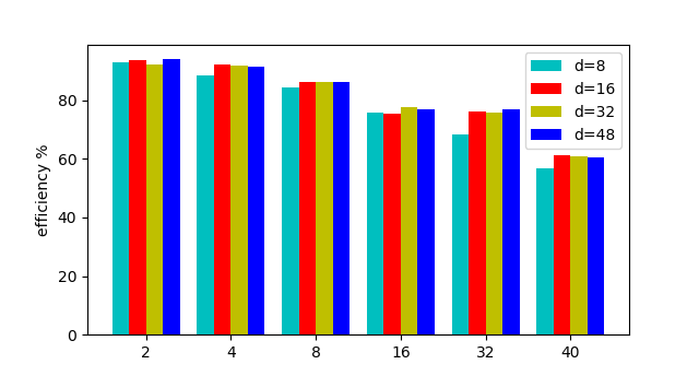
Figure 1: Efficiency plots for evaluation and differentiation of power series, with data from Table 1. Efficiency tends to decrease for increasing $p$. The efficiency improves a little as the truncation degree $d$ of the series increases from 8, 16, 32, to 48.

The drop in efficiency with $p=40$ is because the problem size $n=64$ is not a multiple of $p$, which results in load imbalancing. As quad double arithmetic is already very computationally intensive, the increase in the truncation degree $d$ does little to improve the efficiency. Using more threads increases the memory usage, as each thread needs its own work space for all data structures used in the computation of its gradient with algorithmic differentiation. In a sequential computation where gradients are computed one after the other, there is only one vector with forward, backward, and cross products. When $p$ gradients are computed simultaneously, there are $p$ work space vectors to store the intermediate forward, backward, and cross products for each gradient. The portion of the parallel code that allocates and deallocates all work space vectors grows as the number of threads increases and the wall clock times incorporate the time spent on that data management as well.

5.1.2 Jacobians, Hessians at a Point, and Singular Values

Table 2 summarizes runs on the evaluation and singular value computations on random input data, for $n$-dimensional problems. The $n$ polynomials have each $n$ terms, where the exponents of the variables range from zero to eight.

		double			double double			quad double
$n$	$p$	time	$S(p)$	$E(p)$	time	$S(p)$	$E(p)$	time	$S(p)$	$E(p)$
64	1	0.729			3.964			51.998
	2	0.521	1.40	70.0%	2.329	1.70	85.1%	29.183	1.78	89.1%
	4	0.308	2.37	59.2%	1.291	3.07	76.8%	16.458	3.16	79.0%
	8	0.208	3.50	43.7%	0.770	5.15	64.3%	9.594	5.42	67.8%
	16	0.166	4.39	27.4%	0.498	7.96	49.8%	6.289	8.27	51.7%
	32	0.153	4.77	14.9%	0.406	9.76	30.5%	4.692	11.08	34.6%
	40	0.129	5.65	14.1%	0.431	9.19	23.0%	4.259	12.21	30.5%
96	1	3.562			18.638			240.70
	2	2.051	1.74	86.8%	11.072	1.68	84.17%	132.76	1.81	90.7%
	4	1.233	2.89	72.2%	5.851	3.19	79.64%	72.45	3.32	83.1%
	8	0.784	4.54	56.8%	3.374	5.52	69.06%	41.20	5.84	73.0%
	16	0.521	6.84	42.7%	2.188	8.52	53.25%	25.87	9.30	58.1%
	32	0.419	8.50	26.6%	1.612	11.56	36.13%	15.84	15.20	47.5%
	40	0.398	8.94	22.4%	1.442	12.92	32.31%	15.84	15.20	38.0%
128	1	12.464			62.193			730.50
	2	6.366	1.96	97.9%	33.213	1.87	93.6%	399.98	1.83	91.3%
	4	3.570	3.49	87.3%	17.436	3.57	89.2%	213.04	3.43	85.7%
	8	2.170	5.75	71.8%	9.968	6.24	78.0%	119.81	6.10	76.2%
	16	1.384	9.01	56.3%	6.101	10.19	63.7%	73.09	9.99	62.5%
	32	1.033	12.06	37.7%	4.138	15.03	47.9%	43.44	16.82	52.6%
	40	0.981	12.70	31.7%	3.677	16.92	42.3%	42.44	17.21	43.0%

Table 2: Evaluation of Jacobian and Hessian matrices at a point, singular value decompositions, for $p$ threads, in double, double double, and quad double precision.

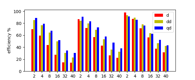
Figure 2: Efficiency plots for computing Jacobians, Hessians, and their singular values, with data from Table 2. The three ranges for $p=2,4,8,16,32,40$ are from left to right for $n=64,96$, and 128 respectively. Efficiency decreases for increasing values of $p$. Efficiency increases for increasing values of $n$ and for increased precision, where d = double, dd = double double, and qd = quad double.

Reading the columns of Table 2 vertically, we observe increasing speedups, which increase as $n$ increases. Reading Table 2 horizontally, we observe the cost overhead of the arithmetic. To see how many threads are needed to compensate for this overhead, read Table 2 diagonally. Figure 2 shows the efficiencies.

To explain the drop in efficiencies we apply the same reasoning as before and point out that the work space increases even more as more threads are applied, because the total memory consumption has increased with the two dimensional Hessian matrices.

5.1.3 Pipelined Solution of Matrix Series

Elapsed wall clock times and speedups are listed in Table 3, on randomly generated linear systems of 64 equations in 64 unknowns, for series truncated to increasing degrees. The dimensions are consistent with the setup of Table 1, to relate the cost of linear system solving to the cost of evaluation and differentiations. Figure 3 shows the efficiencies.

	$d=8$			$d=16$			$d=32$			$d=48$
$p$	time	$S(p)$	$E(p)$	time	$S(p)$	$E(p)$	time	$S(p)$	$E(p)$	time	$S(p)$	$E(p)$
1	0.232			0.605			2.022			4.322
2	0.222	1.05	52.4%	0.422	1.44	71.7%	1.162	1.74	87.0%	2.553	1.69	84.7%
4	0.218	1.07	26.6%	0.349	1.74	43.4%	0.775	2.61	65.3%	1.512	2.86	71.5%
8	0.198	1.18	14.7%	0.291	2.08	26.0%	0.554	3.65	45.6%	0.927	4.66	58.3%
16	0.166	1.40	8.7%	0.225	2.69	16.8%	0.461	4.39	27.5%	0.636	6.80	42.5%
32	0.197	1.18	3.7%	0.225	2.69	8.4%	0.371	5.45	17.0%	0.554	7.81	24.4%
40	0.166	1.40	3.5%	0.227	2.67	6.7%	0.369	5.48	13.7%	0.531	8.14	20.3%

Table 3: Solving a linear system for power series truncated at increasing degrees $d$, for increasing number of threads $p$, in quad double precision.

Consistent with the above analysis, the speedups in Table 3 level off for $p>d/2$. A diagonal reading shows that with multithreading, we can keep the time below one second, while increasing the degree of the truncation from 8 to 48. Relative to the cost of evaluation and differentiation, the seconds in Table 3 are significantly smaller than the seconds in Table 1.

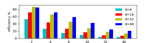
Figure 3: Efficiency plots for pipelined solution of a matrix series with data from Table 3. Efficiency tends to decrease for increasing $p$ and increase for increasing $d$.

5.1.4 Multithreaded Newton’s Method on Power Series

In the randomly generated problems, we add the parameter $t$ to every polynomial to obtain a Newton homotopy. The elapsed wall clock times in Table 4 come from running Newton’s method, which requires the repeated evaluation, differentiation, and linear system solving. The dimensions of the randomly generated problems are 64 equations in 64 variables, with 8 as the highest degree in each variable. The parameter $t$ appears with degree one. Figure 4 shows the efficiencies.

	$d=8$			$d=16$			$d=32$			$d=48$
$p$	time	$S(p)$	$E(p)$	time	$S(p)$	$E(p)$	time	$S(p)$	$E(p)$	time	$S(p)$	$E(p)$
1	347.854			1176.887			4525.080			7005.914
2	188.922	1.84	92.1%	658.935	1.79	89.3%	2323.203	1.95	97.4%	3806.198	1.84	92.0%
4	98.281	3.54	88.5%	330.497	3.56	89.0%	1193.762	3.79	94.8%	1925.040	3.64	91.0%
8	54.551	6.38	79.7%	191.575	6.14	76.8%	638.208	7.09	88.6%	1014.856	6.90	86.3%
16	31.262	11.13	69.5%	97.342	12.09	75.6%	352.103	12.85	80.3%	571.258	12.26	76.7%
32	17.624	19.74	61.7%	50.809	23.16	72.4%	180.318	25.60	78.4%	291.923	24.00	75.0%
40	17.456	19.93	49.8%	51.701	22.76	56.9%	181.563	24.92	62.3%	292.552	23.95	59.9%

Table 4: Running 8 steps with Newton’s method for power series truncated at increasing degrees $d$, for increasing number of threads $p$, in quad double precision.

The improvement in the efficiencies as the degrees increase can be explained by the improvement in the efficiencies in the pipelined solution of matrix series, see Figure 3.

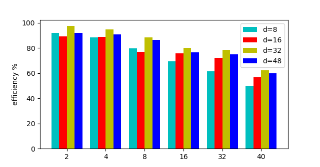
Figure 4: Efficiency plots for running Newton’s method with data from Table 4. Efficiency tends to decrease for increasing $p$ and increase for increasing degree $d$.

5.1.5 Rational Approximations

In Table 5, wall clock times and speedups are listed for the construction and evaluation of vectors of Padé approximants, of dimension 64 and for increasing degrees $d=8,16,24$, and $32$. For each $d$, we take $K=L=d/2$. Figure 5 shows the efficiencies. The fast drop in efficiency for $d=8$ is due to the tiny wall clock times. There is not much that can be improved with multithreading once the time drops below 10 milliseconds.

	$d=8$			$d=16$			$d=32$			$d=48$
$p$	time	$S(p)$	$E(p)$	time	$S(p)$	$E(p)$	time	$S(p)$	$E(p)$	time	$S(p)$	$E(p)$
1	0.034			0.109			0.684			2.193
2	0.025	1.36	68.1%	0.110	0.99	49.4%	0.452	1.51	75.6%	1.231	1.78	89.1%
4	0.013	2.61	65.2%	0.064	1.71	42.6%	0.238	2.87	71.8%	0.642	3.42	85.4%
8	0.007	4.79	59.8%	0.035	3.07	38.4%	0.189	3.63	45.4%	0.365	6.01	75.1%
16	0.006	6.09	38.1%	0.020	5.52	34.5%	0.098	6.96	43.5%	0.219	10.00	62.5%
32	0.004	9.47	29.6%	0.013	8.66	27.1%	0.058	11.70	36.6%	0.138	15.89	49.7%
40	0.003	11.48	28.7%	0.009	11.57	28.9%	0.039	17.58	43.9%	0.130	16.93	42.3%

Table 5: Construction and evaluation of Padé approximants for increasing degrees $d$, for increasing number of threads $p$, in quad double precision.

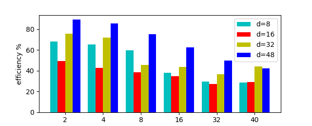
Figure 5: Efficiency plots for rational approximations with data from Table 5.

5.1.6 Shifting the Coefficients of the Power Series

Table 6 summarizes experiments on a randomly generated system of 64 polynomials in 64 unknowns, with 64 terms in every polynomial. Figure 6 shows the efficiencies.

	$d=8$			$d=16$			$d=32$			$d=48$
$p$	time	$S(p)$	$E(p)$	time	$S(p)$	$E(p)$	time	$S(p)$	$E(p)$	time	$S(p)$	$E(p)$
1	0.358			1.667			9.248			26.906
2	0.242	1.48	74.0%	0.964	1.73	86.5%	5.134	1.80	90.1%	14.718	1.83	91.4%
4	0.154	2.32	58.0%	0.498	3.35	83.8%	2.642	3.50	87.5%	7.294	3.69	92.2%
8	0.101	3.55	44.4%	0.289	5.77	72.1%	1.392	6.64	83.0%	3.941	6.83	85.3%
16	0.058	6.13	38.3%	0.181	9.23	57.7%	0.788	11.73	73.3%	2.307	11.66	72.9%
32	0.035	10.30	32.2%	0.116	14.40	45.0%	0.445	20.80	65.0%	1.212	22.20	69.4%
40	0.031	11.49	28.7%	0.115	14.51	36.3%	0.419	22.05	55.1%	1.156	23.28	58.2%

Table 6: Shifting the coefficients of a polynomial homotopy, for increasing degrees $d$, for increasing number of threads $p$, in quad double precision.

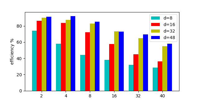
Figure 6: Efficiency plots for shifting series of a polynomial homotopy with data from Table 6. Efficiency tends to decrease for increasing $p$ and increase for increasing $d$.

5.1.7 Proportional Costs

Comparing the times in Tables 1, 2, 3, 5, and 6, we get an impression on the relative costs of the different tasks. The evaluation and differentiation at power series, truncated at $d=8$ dominates the cost with 348 seconds for one thread, or 17 seconds for 40 threads, in quad double arithmetic, from Table 1. The second largest cost comes from Table 2, for $n=64$, in quad double arithmetic: 52 seconds for one thread, or 4 seconds on 40 threads. The other three stages take less than one second on one thread.

5.2 One Cyclic $n$-Root, $n=64,96,128$

Our algorithms are developed to run on highly nonlinear problems such as the cyclic $n$-roots problem:

$$\left\{\begin{array}[]{c}x_{0}+x_{1}+\cdots+x_{n-1}=0\\ i=2,4,\ldots,n-1:\displaystyle\sum_{j=0}^{n-1}~{}\prod_{k=j}^{j+i-1}x_{k~{}{\rm mod}~{}n}=0\\ x_{0}x_{1}x_{2}\cdots x_{n-1}-1=0.\\ \end{array}\right.$$ (34)

This well known benchmark problem in polynomial system solving is important in the study of biunimodular vectors [10].

5.2.1 Problem Setup

By Backelin’s Lemma [2], we know there is a 7-dimensional surface of cyclic 64-roots, along with a recipe to generate points on this surface. To generate points, a tropical formulation of Backelin’s Lemma [1] is used. The surface has degree eight. Seven linear equations with random complex coefficients are added to obtain isolated points on the surface. The addition of seven linear equations gives 71 equations in 64 variables. As in [17], we add extra slack variables in an embedding to obtain an equivalent square 71-dimensional system. Similary, there is a 3-dimensional surface of cyclic 96-roots and again a 7-dimensional surface of cyclic 128-roots.

In [23], running the typical predictor-corrector methods, we experienced that the hardware double precision is no longer sufficient to track a solution path on this 7-dimensional surface of cyclic 64-roots. Observe the high degrees of the polynomials in (34).

Table 7 contains wall clock times, speedups and efficiencies for computing the curvature bound $C$ for one cyclic $n$-root. Efficiencies are shown in Figure 7. Table 8 contains wall clock times, speedups and efficiencies for computing the radius bound $R$ for one cyclic $n$-root. See Figure 8.

	$n=64$			$n=96$			$n=128$
$p$	time	$S(p)$	$E(p)$	time	$S(p)$	$E(p)$	time	$S(p)$	$E(p)$
1	36.862			152.457			471.719
2	21.765	1.69	84.7%	87.171	1.75	87.5%	262.678	1.80	89.8%
4	12.390	2.98	74.4%	47.268	3.23	80.6%	143.262	3.29	82.3%
8	7.797	4.73	59.1%	28.127	5.42	67.8%	83.044	5.68	71.0%
16	5.600	6.58	41.1%	18.772	8.12	50.8%	53.235	8.86	55.4%
32	4.059	9.08	28.4%	12.988	11.74	36.7%	34.800	13.56	42.4%
40	4.046	9.11	22.8%	12.760	11.95	29.9%	33.645	14.02	35.1%

Table 7: Computing $C$ for one cyclic $n$-root, for $n=64$, 96, 128, for an increasing number of threads $p$, in quad double precision.

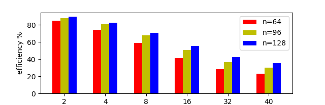
Figure 7: Efficiency plots for computing $C$ for one cyclic $n$-root, for $n=64$, 96, 128, with data from Table 7. Efficiency decreases for increasing $p$ and increases for increasing $n$.

		$n=64$			$n=96$			$n=128$
$d$	$p$	time	$S(p)$	$E(p)$	time	$S(p)$	$E(p)$	time	$S(p)$	$E(p)$
8	1	139.185			483.137			1123.020
	2	78.057	1.78	89.2%	257.023	1.88	94.0%	614.750	1.83	91.3%
	4	42.106	3.31	82.6%	141.329	3.42	85.5%	318.129	3.53	88.3%
	8	24.452	5.69	71.2%	81.308	5.94	74.3%	176.408	6.37	79.6%
	16	15.716	8.86	55.4%	47.585	10.15	63.5%	105.747	10.62	66.4%
	32	12.370	11.25	35.2%	35.529	13.60	42.5%	68.025	16.51	51.6%
	40	12.084	11.52	28.8%	35.212	13.72	34.3%	62.119	18.08	45.2%
16	1	477.956			1606.174			3829.567
	2	256.846	1.86	93.0%	861.214	1.87	93.3%	2066.680	1.85	92.7%
	4	136.731	3.50	87.4%	454.917	3.53	88.3%	1072.106	3.57	89.3%
	8	77.034	6.20	77.6%	251.066	6.40	80.0%	584.905	6.55	81.8%
	16	47.473	10.07	62.9%	149.288	10.76	67.2%	344.430	11.12	69.5%
	32	32.744	14.60	45.6%	97.514	16.47	51.5%	205.034	18.68	58.4%
	40	32.869	14.54	36.4%	89.260	18.00	45.0%	180.207	21.25	53.1%
24	1	1023.968			3420.576			8146.102
	2	555.771	1.84	92.1%	1855.748	1.84	92.2%	4360.870	1.87	93.4%
	4	304.480	3.36	84.1%	956.443	3.58	89.4%	2268.632	3.59	89.8%
	8	160.978	6.36	79.5%	523.763	6.53	81.6%	1235.338	6.59	82.4%
	16	98.336	10.41	65.1%	312.698	10.94	68.4%	726.287	11.22	70.1%
	32	65.448	15.65	48.9%	196.488	17.41	54.4%	416.735	19.55	61.1%
	40	63.412	16.15	40.4%	170.474	20.07	50.2%	360.419	22.60	56.5%

Table 8: Computing $R$ for one cyclic $n$-root, for $n=64$, 96, 128, for degrees $d=8,16,24$, and for an increasing number of threads $p$, in quad double precision.

For $n=64$, the inverse condition number of the Jacobian matrix is estimated as $3.9\mathrm{E}{-5}$ and after 8 iterations, the maximum norm of the last vector in the last update to the series equals respectively $4.6\mathrm{E}{-44}$, $1.1\mathrm{E}{-24}$, and $4.1\mathrm{E}{-5}$, for $d=8,16$, and 24. For $n=96$, the estimated inverse condition number is $2.0\mathrm{E}{-4}$ and the maximum norm for $d=8,16$, and 24 is then respectively $1.4\mathrm{E}{-47}$, $9.6\mathrm{E}{-31}$, and $7.3\mathrm{E}{-14}$. The condition worsens for $n=128$, estimated at $4.6\mathrm{E}{-6}$ and then for $d=8$, the maximum norm of the last update vector is $2.2\mathrm{E}{-30}$. For $d=16$ and 24, the largest maximum norm less than one occurs at the coefficients with $t^{15}$ and equals about $1.1\mathrm{E}{-1}$.

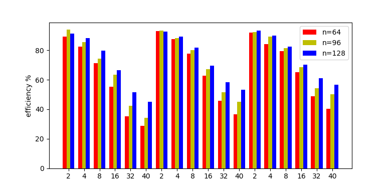
Figure 8: Efficiency plots for computing $R$ for one cyclic $n$-root, for $n=64$, 96, 128, for degrees $d=8$, 16, 24, with data from Table 7. Efficiency decreases for increasing $p$. Efficiency increases as $n$ and/or $d$ increase.

6 Conclusions

The cost overhead of our robust path tracker is $O(n)$, compared with the current numerical predictor-corrector algorithms. For $n=64$, we expect a cost overhead factor of about 64. We interpret the speedups in Table 7 and Table 8 as follows. With a speedup of about 10, then this factor drops to about 6.

The plan is to integrate the new algorithms in the parallel blackbox solver [22].

References

- [1] D. Adrovic and J. Verschelde. Polyhedral methods for space curves exploiting symmetry applied to the cyclic -roots problem. In Computer Algebra in Scientific Computing, 15th International Workshop, CASC 2013, pages 10–29. Springer-Verlag, 2013.
- [2] J. Backelin. Square multiples n give infinitely many cyclic n-roots. Reports, Matematiska Institutionen 8, Stockholms universitet, 1989.
- [3] D. J. Bates, J. D. Hauenstein, A. J. Sommese, and C. W. Wampler. Adaptive multiprecision path tracking. SIAM J. Numer. Anal., 46(2):722–746, 2008.
- [4] D. J. Bates, J. D. Hauenstein, A. J. Sommese, and C. W. Wampler. Numerically Solving Polynomial Systems with Bertini, volume 25. SIAM, 2013.
- [5] N. Bliss and J. Verschelde. The method of Gauss–Newton to compute power series solutions of polynomial homotopies. Linear Algebra Appl., 542:569–588, 2018.
- [6] P. Breiding and S. Timme. HomotopyContinuation.jl: A package for homotopy continuation in Julia. In International Congress on Mathematical Software, pages 458–465. Springer, 2018.
- [7] B. Christianson. Automatic Hessians by reverse accumulation. IMA Journal of Numerical Analysis 12:135–150, 1992.
- [8] J. H. Davenport. Looking at a set of equations. Bath Computer Science Technical Report 87-06, 1987.
- [9] E. Fabry. Sur les points singuliers d’une fonction donnée par son développement en série et l’impossibilité du prolongement analytique dans des cas très généraux. In Annales scientifiques de l’École Normale Supérieure, volume 13, pages 367–399. Elsevier, 1896.
- [10] H. Führ and Z. Rzeszotnik. On biunimodular vectors for unitary matrices. Linear Algebra Appl., 484:86–129, 2015.
- [11] A. Griewank and A. Walther. Evaluating derivatives: principles and techniques of algorithmic differentiation, volume 105. SIAM, 2008.
- [12] Y. Hida, X. S. Li, and D. H. Bailey. Algorithms for quad-double precision floating point arithmetic. In the Proceedings of the 15th IEEE Symposium on Computer Arithmetic (Arith-15 2001), pages 155–162. IEEE Computer Society, 2001.
- [13] G. Jeronimo, G. Matera, P. Solernó, and A. Waissbein. Deformation techniques for sparse systems. Found. Comput. Math., 9:1–50, 2009.
- [14] S. Katsura. Spin glass problem by the method of integral equation of the effective field. In M. Coutinho-Filho and S. Resende, editors, New Trends in Magnetism, pages 110–121. World Scientific, 1990.
- [15] T. Li and C. Tsai. HOM4PS-2.0para: Parallelization of HOM4PS-2.0 for solving polynomial systems. Parallel Computing, 35(4):226–238, 2009.
- [16] J. W. McCormick, F. Singhoff, and J. Hugues. Building Parallel, Embedded, and Real-Time Applications with Ada. Cambridge University Press, 2011.
- [17] A.J. Sommese and J. Verschelde. Numerical homotopies to compute generic points on positive dimensional algebraic sets. J. of Complexity, 16(3):572–602, 2000.
- [18] S. Telen, M. Van Barel, and J. Verschelde. A Robust Numerical Path Tracking Algorithm for Polynomial Homotopy Continuation. arXiv:1909.04984.
- [19] A. Trias. The holomorphic embedding load flow method. In 2012 IEEE Power and Energy Society General Meeting, pages 1–8. IEEE, 2012.
- [20] A. Trias and J. L. Martin. The holomorphic embedding loadflow method for DC power systems and nonlinear DC circuits. IEEE Transactions on Circuits and Systems, 63(2):322–333, 2016.
- [21] J. Verschelde. Algorithm 795: PHCpack: A general-purpose solver for polynomial systems by homotopy continuation. ACM Transactions on Mathematical Software (TOMS), 25(2):251–276, 1999.
- [22] J. Verschelde. A blackbox polynomial system solver on parallel shared memory computers. In Computer Algebra in Scientific Computing, 20th International Workshop, CASC 2018, pages 361–375. Springer-Verlag, 2018.
- [23] J. Verschelde and X. Yu. Accelerating polynomial homotopy continuation on a graphics processing unit with double double and quad double arithmetic. In Proceedings of the 7th International Workshop on Parallel Symbolic Computation (PASCO 2015), pages 109–118. ACM, 2015.