Quantum Coherence in Ergodic and Many-Body Localized Systems

Abstract

Quantum coherence quantifies the amount of superposition a quantum state can have in a given basis. Since there is a difference in the structure of eigenstates of the ergodic and many-body localized systems, we expect them also to differ in terms of their coherences in a given basis. Here, we numerically calculate different measures of quantum coherence in the excited eigenstates of an interacting disordered Hamiltonian as a function of the disorder. We show that quantum coherence can be used as an order parameter to detect the well-studied ergodic to many-body-localized phase transition. We also perform quantum quench studies to distinguish the behavior of coherence in thermalized and localized phases. We then present a protocol to calculate measurement-based localizable coherence to investigate the thermal and many-body localized phases. The protocol allows one to investigate quantum correlations experimentally in a non-destructive way, in contrast to measures that require tracing out a subsystem, which always destroys coherence and correlation.

I Introduction

Advances in experimental realizations of closed quantum many-body systems such as ultra-cold atoms, trapped ions, or superconducting qubits undergoing unitary evolution over long time scales Bloch et al. (2008, 2012); Blatt and Roos (2012); Georgescu et al. (2014); Guo et al. (2019) have lead to the study of quantum dynamical phenomena like dynamical quantum phase transitions,Jurcevic et al. (2017); Zhang et al. (2017) discrete time crystals,Choi et al. (2017) and many-body localization (MBL).Schreiber et al. (2015) One of the main focuses of these studies is to examine the way isolated systems reach thermal equilibrium. Deutsch Deutsch (1991) and Srednicki Srednicki (1994) discussed the process of thermalization and the eigenstate thermalization hypothesis (ETH) Srednicki (1994) was put forward as a strong criterion for thermalization to occur in closed quantum many-body systems. MBL Basko et al. (2006); Gornyi et al. (2005); Oganesyan and Huse (2007); Nandkishore and Huse (2015); Pal and Huse (2010); Vosk and Altman (2013); Ponte et al. (2015) has emerged as an extension of the much-studied Anderson localization,Anderson (1958) applicable in the case of closed interacting systems. MBL systems fail to thermalize due to the presence of local integrals of motion Chandran et al. (2015); Huse et al. (2014); Serbyn et al. (2013a) and hence the MBL eigenstates violate the ETH hypothesis, according to which all the eigenstates of a thermalizing system have to be locally thermal. ETH also postulates that the matrix elements of any local observable $O$, between two eigenstates $i,j$ of the Hamiltonian can be expressed as $\left\langle{i}\right|{O}\left|{j}\right\rangle=O(\bar{E})\delta_{ij}+\exp(-S(\bar{E})/2)f_{O}(\bar{E},\omega)R_{ij}$, where $\bar{E}\equiv(E_{i}+E_{j})/2,\omega=E_{j}-E_{i},$ and $S(E)$ is the thermodynamic entropy at energy $E$. It is also important to note that both $O(\bar{E})$ and $f_{O}(\bar{E},\omega)$ are smooth functions of their arguments and $R_{ij}$ is a random real or complex variable with zero mean and unit variance.

The effort of keeping a quantum system decoupled from the environment and thus undergoing unitary dynamics is done with the goal of preserving coherence in the many-body wave-function. Coherence quantifies the amount of superposition of a particular state in any fixed basis sets. A rigorous framework for quantum coherence as a resource has been developed recently.Streltsov et al. (2017); Chitambar and Hsieh (2016); Chitambar and Gour (2016); Baumgratz et al. (2014) The study of quantum coherence in closed quantum systems is relevant because quantum coherence is exactly what is responsible for quantum fluctuations and correlations. In a many-body quantum system, local degrees of freedom are described by a tensor product structure (TPS). Coherent superposition of basis states in a TPS results in quantum entanglement and this is why, in recent years, entanglement has been widely studied as a diagnostic tool for quantum phase transitions in many-body systems Eisert et al. (2010) or as a probe to exotic quantum orders like topological order.Hamma et al. (2005a, b, c); Flammia et al. (2009); Wen (2007); Kitaev and Preskill (2006); Levin and Wen (2006) In the context of the ETH-MBL phase transition in spin chains, entanglement has been used as a useful marker of the transition.Luitz et al. (2015); Sierant and Zakrzewski (2019); Yang et al. (2017); Potter et al. (2015) In quantum many-body dynamics, the nature of the growth of entanglement entropy has been considered as an important tool for characterizing different dynamical phases. It has been shown that MBL offers slow logarithmic growth while ETH has a linear growth of entanglement entropy.Bardarson et al. (2012); Serbyn et al. (2013b)

In this paper, we study the role that quantum coherence plays in the MBL-ETH transition. As coherence is a function of the wave function, one should expect that some of its moments should be able to capture any kind of transition. We first show that coherence (in the computational basis) in a high energy eigenstate and its variance due to sample-to-sample fluctuations do indeed signal the MBL-ETH transition. Second, we look at the coherence/decoherence power of dynamics generated by MBL and ETH Hamiltonians. We find that ergodic dynamics induced by ETH has more coherence/decoherence power in a basis that is incompatible with that of the energy, while the dynamics induced by MBL has a low coherence/decoherence power, or, in other words, retains memory of the initial conditions.

However, quantum coherence does not contain any information about the TPS and is, by itself, useless to discriminate the localized versus unlocalized structure of quantum states. To this end, we exploit the notion of localizable coherence that has recently been put forward in Ref. Hamma et al., 2020. Localizing coherence to two blocks of spins, we can then compute the coherence in these two blocks as a function of their distance $d(A,B)$, as a coherence-connected correlation function $C_{d}$. We show that while this quantity does depend on $d$ within the dynamics induced by a MBL Hamiltonian, the ergodic dynamics induced by the ETH Hamiltonian is insensitive to the distance between the two blocks. We finally note that due to the projective nature of coherence measures, they are more suitable to experimental investigation than entanglement entropy, making our results amenable to testing beyond numerical computations.

II Measures of quantum coherence

Quantum coherence is a notion relative to a specific basis. A (Hermitian) operator is called incoherent if it is diagonal in a particular basis $B=\{\left|{i}\right\rangle\}$. We call $I_{B}$ the set of incoherent states in $B$. As an example, the Gibbs state is incoherent in the energy eigenbasis $E$ since its completely diagonal in it. Every completely dephased operator in $B$ is also incoherent in that basis. The set $I_{B}$ is given by just any probability distribution over $\pi_{i}$, where $\pi_{i}=\left|{i}\right\rangle\left\langle{i}\right|$ are the projectors in the basis $B$. Thus we can say that any completely dephased operator $X\in I_{B}$ can be expressed as $X=\sum_{i}p_{i}\pi_{i}$. Therefore, a coherence measure for a state $\rho$ is the quantity

$$C_{B,l_{p}}(\rho):=\|\rho-\mathcal{D}_{B}(\rho)\|_{l_{p}},$$ (1)

where $\mathcal{D}_{B}(\rho)=\sum_{i}\pi_{i}\rho\pi_{i}$ is the completely dephased state and the measure is based on the $l_{p}$ norm. According to this definition, a state $\rho$ has zero coherence, $C_{B}(\rho)=0$, if and only if $\rho\in I_{B}$. We use two different matrix norms as measure for coherence.Streltsov et al. (2017); Baumgratz et al. (2014) Using the $l_{1}$ norm, coherence is expressed as the sum of all the off-diagonal elements of the quantum state, that is, $C_{B,l_{1}}(\rho)=\sum_{i\neq j}|\langle i|\rho|j\rangle|$. Similarly, using the $l_{2}$ norm measure we obtain $C_{B,l_{2}}(\rho)=\sum_{i\neq j}|\langle i|\rho|j\rangle|^{2}$.

Another way of measuring coherence in a basis $B$, which we also employ, is through the Kullback-Leibler divergence from the completely dephased state,

$$C_{B}^{\rm KL}(\rho):=S(\mathcal{D}_{B}(\rho))-S(\rho),$$ (2)

where $S(\rho)$ indicates the entropy of the state $\rho$.

III Quantum Coherence in disordered spin chain

In order to study the role of coherence in the ETH-MBL transition, we consider the disordered Heisenberg $1/2$-spin chain Žnidarič et al. (2008) described by the Hamiltonian

$$H=\sum_{i=1}^{N}J(S_{i}^{x}S_{i+1}^{x}+S_{i}^{y}S_{i+1}^{y}+S_{i}^{z}S_{i+1}^{z})+h_{i}S_{i}^{z}+h_{x}S_{i}^{x}$$ (3)

with periodic boundary conditions. We set $J=1$ in the numerical computation. The static random fields $h_{i}$ are chosen from a uniform distribution in $[-W,W]$. A transverse constant field $h_{x}=0.1$ is introduced to break the total $S_{z}$ conservation so that no sector with conserved quantities that break ergodicity explicitly exist.Regnault and Nandkishore (2016); Yang et al. (2017)

III.1 ETH-MBL transition point from level statistics

The model Hamiltonian in Eq. (3) without the small transverse field ($h_{x}$) is known to undergo an ergodic to MBL transition for strong disorder.Pal and Huse (2010); Sierant and Zakrzewski (2019); Luitz et al. (2015) Here, in order to locate transition point between the eigenstate thermalization hypothesis (ETH) to many-body localization (MBL) regimes, we diagonalize the full Hamiltonian in Eq. (3) and calculate the energy level spacing $\delta_{\alpha}^{n}=|E_{\alpha}^{n}-E_{\alpha}^{n+1}|$, where $E_{\alpha}^{n}$ is the energy of the $n$-th eigenstate in the $\alpha$-th disorder sample. The ratio of the adjacent gaps or level spacings $r_{\alpha}^{n}=\mbox{min}\{\delta_{\alpha}^{n},\delta_{\alpha}^{n+1}\}/\mbox{max}\{\delta_{\alpha}^{n},\delta_{\alpha}^{n+1}\}$ is averaged over the samples to yield $\langle r_{\rm avg}\rangle$. In random matrix theory, when the statistical distribution of level spacing follows the the predictions of the Gaussian Orthogonal Ensemble (GOE) $\langle r_{\rm avg}\rangle$ converges to $r_{\rm GOE}\approx 0.53$ for $N\rightarrow\infty$. We find that, deep in the ergodic phase, the average ratio $\langle r_{\rm avg}\rangle$ does approach the GOE (Gaussian Orthogonal Ensemble) value (see Fig. 1). On the other hand, deep in the localized phase, it reaches the value derived from a Poisson distribution of level spacings, and $\langle r_{\rm avg}\rangle$ converges to $r_{\rm Poisson}\approx 0.39$. Finite-size scaling gives an estimate of the critical value of disorder to drive the transition from ETH to MBL at $W\approx 3.5$.

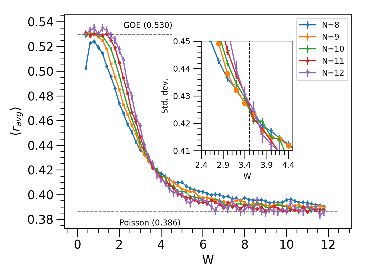
Figure 1: Average level spacing ratio $\langle r_{\rm avg}\rangle$ versus the disorder strength $W$ for different system sizes ($N$ identifies the number of spins in the chain). We obtain $\langle r_{\rm avg}\rangle$ by first averaging over $10$ eigenstates near the middle of the spectrum for each disorder realization and then averaging over different realizations. We employed $8000$ disorder samples for $N=8,9$, $4000$ for $N=10,11$, and $1000$ for $N=12$.

III.2 ETH-MBL transition point from quantum coherence

We now show that one can also extract information about this transition from measures of coherence. Recently,Georgios et al. (2019) it was shown that the escape probability and dynamical conductivity are connected by measures of coherence that can effectively probe the localization transition. Since the ETH and MBL phases are characterized by the different structures of the high-energy eigenstates, we start by evaluating the coherence present in a eigenstate in the middle of the spectrum. As a basis, we choose the computational ($z$) basis for the tensor product of the spins as the preferred basis in which one can observe quantum fluctuations. Here we calculate coherence using $l_{1}$. The disorder-averaged normalized coherence $\langle\mbox{Coh}\rangle=\langle C_{B,l_{1}}(\rho)\rangle/(2^{N}-1)$ for different system sizes feature a crossing at a disorder value around $W=2.5$, see Fig. 2a. The standard deviation of the normalized coherence due to sample-to-sample variations also shows critical behavior around $W=2.5$, see inset in Fig. 2a.

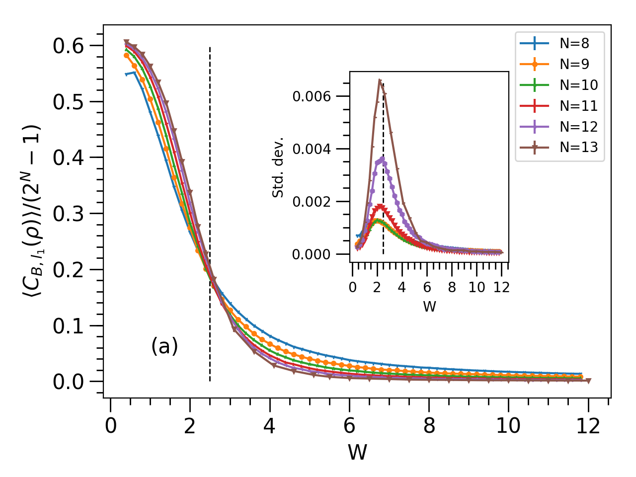
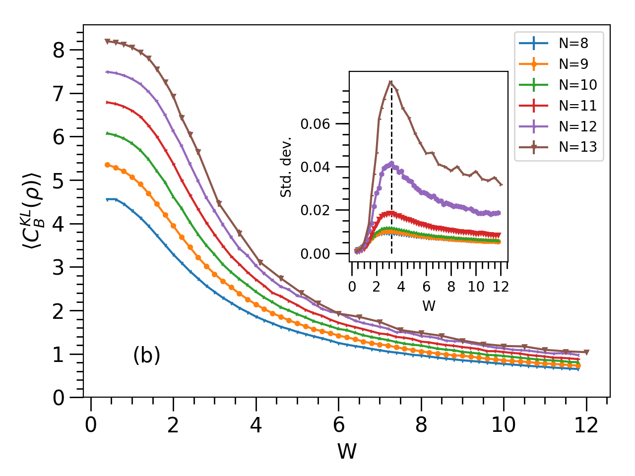
Figure 2: Average normalized coherences: (a) $\langle C_{B,l_{1}}(\rho)\rangle$ and (b) $\langle C_{B}^{\rm KL}(\rho)\rangle$ of an excited state as a function of disorder for different chain sizes. We use the eigenstate exactly at the middle of spectrum for each case. The data are averaged over $8000$ disorder samples for $N=8,9$, $4000$ for $N=10,11$, and $1000$ for $N=12,13$. The inset shows standard deviation of the normalized coherence as a function of disorder for the specific eigenstates mentioned earlier.

Next, we calculate the average Kullback-Leibler divergence between the completely dephased state and a high-energy eigenstate, see Eq. (2). In this case, $\langle C_{B}^{\rm KL}(\rho)\rangle$ does not reveal any crossing point for different system sizes, see Fig. 2b. However, similarly to $\langle C_{B,l_{1}}(\rho)\rangle$ in the inset of Fig. 2a, the standard deviation does show a well-defined peak, but in this case the peak is centered at $W=3.2$ for the system sizes we investigated. Although a peak is much easier to follow and employ for finite-size scaling analyzes than a line crossing (Fig. 1), larger systems would nevertheless be for an accurate estimate of the transition point location.

III.3 Coherence after a quantum quench

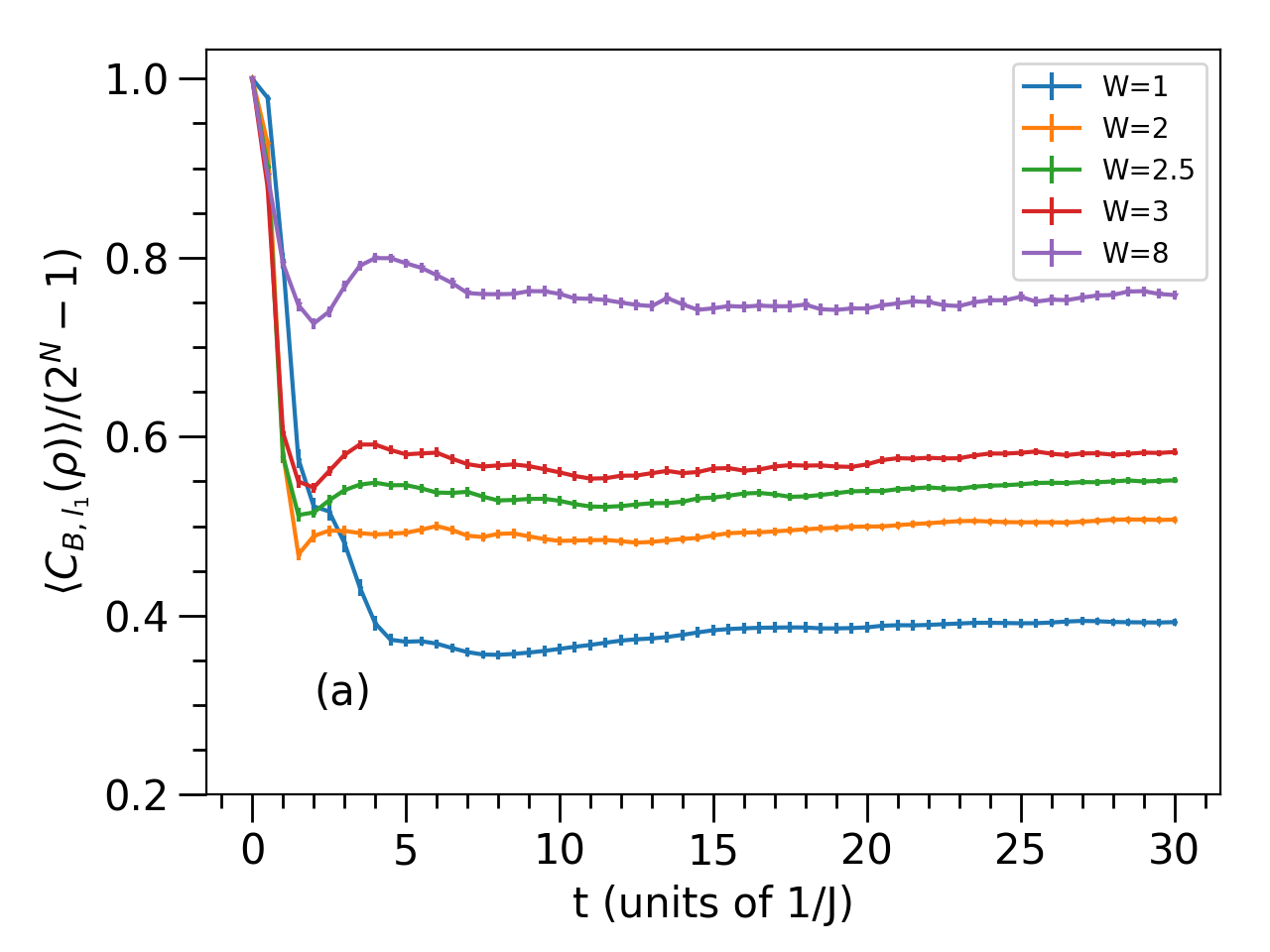
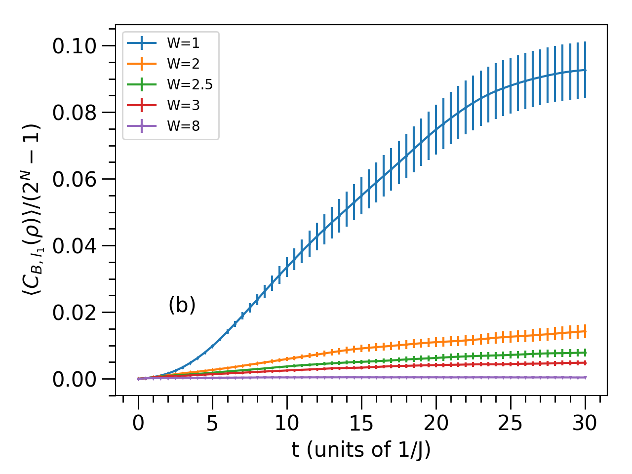
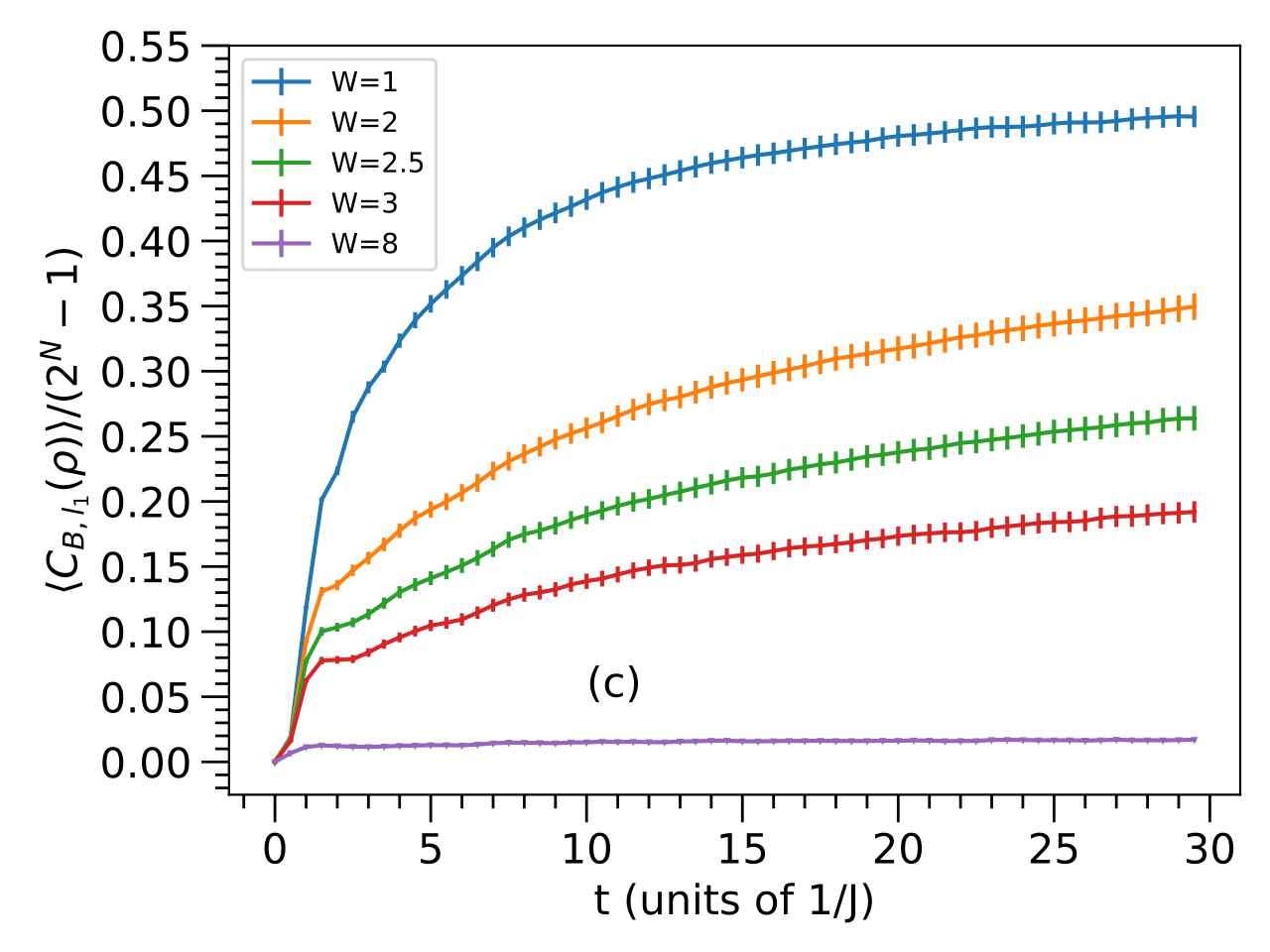
Figure 3: Time evolution of the average normalized coherence $\langle C_{B,l_{1}}(\rho)/(2^{N}-1)\rangle$ starting from: (a) the maximal coherent state $\left|{\Psi}\right\rangle=\frac{1}{\sqrt{d}}\sum_{i=1}^{d}\left|{i}\right\rangle$ in the computational basis, (b) the state $\left|{\Psi}\right\rangle=\left|{\uparrow\uparrow\ldots\uparrow}\right\rangle$, and (c) the state $\left|{\Psi}\right\rangle=\left|{\uparrow\downarrow\uparrow\downarrow\ldots}\right\rangle$. Here, $N=12$ and 200 disorder realizations are employed.

Now consider a situation away from equilibrium, e.g., a quantum quench. After an initial preparation, we let the state evolve unitarily under the Hamiltonian in Eq. (3) for different strengths of the disorder $W$. In the ergodic phase, the long-time evolution should take the state to equilibrate as a thermal ensemble of the eigenstates of the Hamiltonian. Since these are very delocalized in the eigenbasis of the local spins – that is, in the computational basis – we expect that evolution under the ETH Hamiltonian will have more of both coherence and decoherence power than that of the MBL Hamiltonian. We prepare the initial state as either (i) the maximally coherent state $\left|{\Psi}\right\rangle={d}^{-1/2}\sum_{i=1}^{d}\left|{i}\right\rangle$ (in the computational basis), in which case the time evolution will decohere the state; or (ii) an incoherent state, that is, any basis state in the computational basis. We use two different incoherent states to make sure that the behavior of coherence is independent of the initial energy of the system. The results are shown in Fig. 3. We see that the dynamics induced by the ETH and MBL Hamiltonians are strikingly different in terms of the coherence and decoherence power. The ETH Hamiltonian decoheres in a more efficient way a very coherent state, and, at the same time, it is capable of building up more coherence from an incoherent state.

Hence from studying the dynamics of quantum coherence for different initial states, we confirm quite clearly that the MBL phase retains the memory of the initial state.Vasseur et al. (2015); Gopalakrishnan and Parameswaran (2019); Altman and Vosk (2015)

IV Localizable coherence

In a quantum many-body system the Hamiltonian is the sum of local terms, and local terms have support on local Hilbert spaces, e.g., the spins. The total Hilbert space $\mathcal{H}=\otimes_{i}\mathcal{H}_{i}$ is the tensor product of the local Hilbert spaces. In other words, quantum many-body systems create a tensor product structure. Following Ref. Hamma et al., 2020, we want to quantify the coherence that is localizable in a subsystem $S$ comprising a subset of all the spins. For this purpose, we adopt the bipartition $\mathcal{H}=\mathcal{H}_{S}\otimes\mathcal{H}_{R}$ (”system” and ”rest”) with $\mbox{dim}(\mathcal{H})=d=d_{S}\,d_{R}$. We then localize coherence in the subsystem $S$ by performing a measurement on $R$. The latter step consists of the following. Let $B_{R}:=\{\left|{i}\right\rangle\}_{i=1}^{d_{R}}$ be some preferred basis in the subsystem, where $\omega_{i}:=\left|{i}\right\rangle\left\langle{i}\right|$ form a complete set of rank-one projectors over $\mathcal{H_{R}}$. A projective measurement on $\mathcal{H_{R}}$ transforms a density matrix $\rho$ to a tensor product state of the form

$$\rho_{i}^{\prime}=\frac{\text{Tr}_{R}\,(\rho\,I_{S}\otimes\omega_{i})}{\text{Tr}\,(\rho\,I_{S}\otimes\omega_{i})}\otimes\omega_{i}.$$ (4)

Each $\rho_{i}$ is obtained with the probability $p_{i}=\text{Tr}\,(\rho\,I_{S}\otimes\omega_{i})$. One can then trace out the system $R$ without having the state decohere and compute the coherence in $S$ in any basis of the system $B_{S}$, now described by

$$\rho_{S,i}^{\prime}=\text{Tr}_{R}\,\rho_{i}^{\prime}=\frac{\text{Tr}_{R}\,(\rho\,\omega_{i})}{\text{Tr}(\rho\,\omega_{i})}.$$ (5)

Finally, the average coherence in the post-measurement states of the system can be defined as

$$C_{\rm avg}(\rho):=\sum_{i=1}^{d_{R}}p_{i}\,C_{B_{S}}(\rho_{S,i}^{\prime}).$$ (6)

The calculation of the above quantity is carried out using matrix product states (MPS).Verstraete et al. (2008) The protocol of measurement on MPS was first discussed by Popp and coworkers Popp et al. (2005) in the context of localizable entanglement. Here we extend that formalism and calculate the average local coherence for a particular subsystem.

We again consider the disordered Heisenberg spin ${1}/{2}$ in Eq. (3) as a model Hamiltonian. We prepare the initial state in an incoherent state and let it evolve. For the time-evolved state, we calculate the localizable coherence in a subsystem consisting of two blocks $(A,B)$ each consisting of two spins placed at a distance $d(A,B)$ from each other. Our goal is to show that whereas the ergodic delocalized phase should be insensitive to $d(A,B)$, in the MBL phase the localizable coherence should be higher when the two blocks are closer together. In order to localize coherence in the $(A,B)$ blocks, we perform projective measurements in the rest of the system. Let us describe the procedure for the projection in the MPS formalism. Here we consider two blocks to be separated by three spins, $d(A,B)=3$, but we can use similar methods for other separations. The exact quantum state of the $N$-spin system is represented by the so-called MPS,

$$\left|{\Psi}\right\rangle=\sum_{x_{N}=\uparrow,\downarrow}\cdots\sum_{x_{1}=\uparrow\downarrow}M_{N}^{x_{N}}\cdots M_{1}^{x_{1}}\left|{x_{N}\cdots x_{1}}\right\rangle.$$ (7)

Here we will consider the localized coherence between two blocks each consisting of two spins and separated by distance $d(A,B)=3$. Block $A$ consists of matrices $M_{N/2-2}^{x_{N/2-2}}$ and $M_{N/2-1}^{x_{N/2-1}}$. Block $B$ consists of matrices $M_{N/2+2}^{x_{N/2+2}}$ and $M_{N/2+3}^{x_{N/2+3}}$. We calculate all possible projectors on the rest of the system which is given by the tuple $\{s\}=\{x_{N},x_{N-1},\cdots,x_{1}\}-\{x_{N/2-2},x_{N/2-1}\}-\{x_{N/2+2},x_{N/2+3}\}$, consisting of $N-4$ spins. pure state after any projection can be written as

$$\left|{\phi_{\{s\}}}\right\rangle = \left\langle\{s\}|\Psi\right\rangle$$ (9)

$$= \sum_{x_{N/2-2}=\uparrow,\downarrow}\sum_{x_{N/2-1}=\uparrow,\downarrow}\sum_{x_{N/2+2}=\uparrow,\downarrow}\sum_{x_{N/2+3}=\uparrow,\downarrow}R\cdot M_{N/2+3}^{x_{N/2+3}}\,M_{N/2+2}^{x_{N/2+2}}\cdot Q\cdot\ M_{N/2-1}^{x_{N/2-1}}\,M_{N/2-2}^{x_{N/2-2}}\cdot P$$

$$\times\left|{x_{N/2+3},x_{N/2+2}}\right\rangle\left|{x_{N/2-1},x_{N/2-2}}\right\rangle,$$

where the three auxiliary matrices $R$, $Q$ and $P$ are defined as following:

$$R=\sum_{\{x_{N},\ldots,x_{N/2+4}\}}M_{N}^{x_{N}}\cdot M_{N-1}^{x_{N-1}}\cdots M_{N/2+4}^{x_{N/2+4}},$$ (10)

$$Q=\sum_{\{x_{N/2+1},x_{N/2}\}}M_{N/2+1}^{x_{N/2+1}}\cdot M_{N/2}^{x_{N/2}}.$$ (11)

and

$$P=\sum_{\{x_{N/2-3},\ldots,x_{1}\}}M_{N/2-3}^{x_{N/2-3}}\cdots M_{1}^{x_{1}}.$$ (12)

$R$,$Q$ and $P$ are computed by carrying out the matrix multiplications for each tuple $\{x_{N},\cdots,x_{N/2+4}\}=s_{1},\{x_{N/2+1},x_{N/2}\}=s_{2}$, and $\{x_{N/2-3},\cdots,x_{1}\}=s_{3}$ respectively. There are total $2^{N-4}$ possible combinations for $s_{1}$, $s_{2}$, and $s_{3}$ combined, each of which corresponds to a different projector. The probability of a specific projector is then given by

$$\text{Pr}(\{s\})=\left\langle\phi_{\{s\}}|\phi_{\{s\}}\right\rangle=|{\left\langle\{s\}|\Psi\right\rangle}|^{2},$$ (13)

and the density matrix corresponding to the projected pure state is

$$\rho(\{s\})=\frac{1}{\text{Pr}(\{s\})}\left|{\phi_{\{s\}}}\right\rangle\left\langle{\phi_{\{s\}}}\right|.$$ (14)

The average local coherence of the two blocks is then computed according to the expression

$$\text{C}_{l_{2}}(\text{avg})=\sum_{i=1}^{2^{N-4}}\text{Pr}_{i}(\{s\})\times\text{C}_{l_{2}}(\rho_{i}(\{s\})).$$ (15)

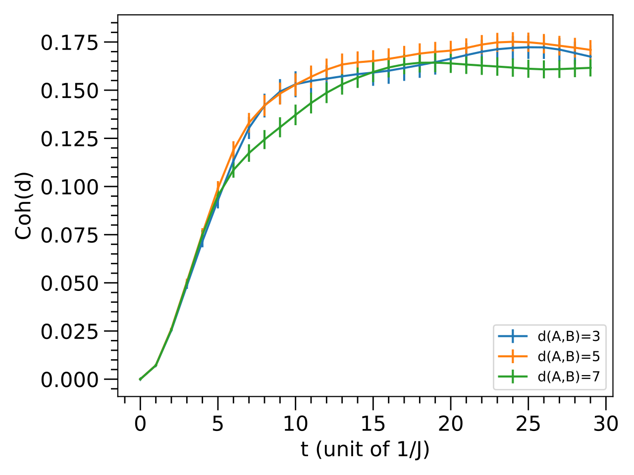
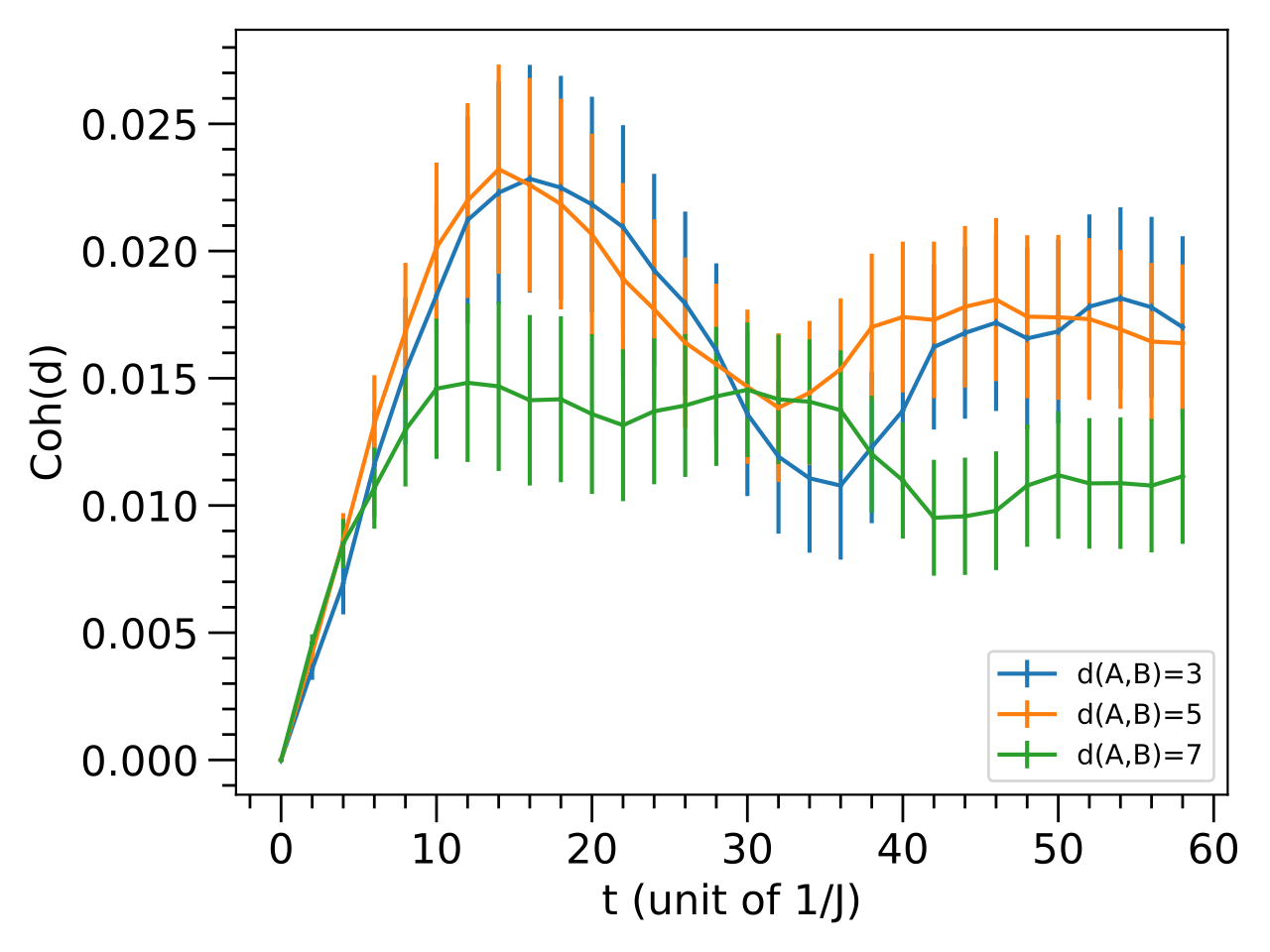
Figure 4: Average localizable coherence after a quantum quench with (a) the ETH Hamiltonian ($W=1$) and (b) the MBL Hamiltonian ($W=10$). The quantity $\langle\mbox{Coh}(d)\rangle$ is computed for two blocks $A$ and $B$ of two spins each at different distance $d(A,B)=3,5,\ldots$. The total number of spins is $N=14$. The initial state is the product state $\left|{\downarrow\downarrow...\downarrow}\right\rangle$. The $l_{2}$ norm of coherence is evaluated in the computational basis. The results represent an average over $480$ disordered samples. In case of the MBL Hamiltonian (b) we perform the quench for a longer time to specify the nature of distance dependence of average localizable coherence over longer timescale.

To obtain the correlation of local coherence among these two-spin blocks one need to subtract the effect of these individual blocks. An effective way to do that is to calculate the local coherence of the two-spin blocks in different locations of the disordered spin chain, while considering the appropriate set of projective measurements on the respective Hilbert spaces, and then take an average over the results. One then subtract the calculated average coherence of the individual blocks from the local coherence of the two two-spin blocks to define $\mbox{Coh}(d)$ as localizable coherence, namely,

$$\text{Coh(d)}=\text{C}_{l_{2}}(\text{avg})-\frac{1}{4}\sum_{i=1}^{4}\text{C}_{l_{2}}(p_{i}).$$ (16)

Here, $\text{C}_{l_{2}}(p_{i})$ refers to the coherence of the individual two-spin blocks in several different locations along the spin chain.

In order to compute the time evolution after the quantum quench we utilize the time-evolving block decimation (TEBD) method.Vidal (2004); Paeckel et al. (2019) For the TEBD, we have used a second order Suzuki-Trotter decomposition with a time step $\delta t=0.1$ and open boundary condition. We let the bond dimension increase to the maximum ($D=2^{N/2}$), which in case of 4 is 128, during time evolution. The time evolution reveals an important feature of the local structure of the wave function in the ETH or MBL phase. In ETH the many-body wave function is extended, resulting in distance-independent behavior of the average local coherence between different blocks, which is clearly shown in Fig. 4a. In contrast, in MBL we can see that the average local coherence between two blocks decreases with distance when they are farther apart than the localization length (see Fig. 4b). Considering these results, we can say that the maximum local coherence of two blocks is higher in ETH than in the MBL phase. Since all the coherence has been measured in the computational basis, the lower local coherence in MBL indicates the localized structure of the wave function in the Hilbert space.

V Conclusions and outlook

In this paper, we show that measures of coherence are effective in distinguishing the ergodic (ETH) and many-body localized (MBL) phases and their dynamics after a quantum quench. In particular, we show that the standard deviation of the coherence and the entropy of coherence for a high-energy eigenstate mark the localization transition. We also show that the time evolution of the coherence characterizes the different dynamics of the two phases. We then utilize a notion of correlation of coherence based on the localizable coherence introduced in Ref. Hamma et al., 2020, to show that the ergodic phase is insensitive to the distance between the subsystems, while it decays for the localized phase.

We conclude that localizable coherence can be a useful instrument in the investigation of quantum many-body systems. For example, one could look at the fluctuations of this quantity as a probe for scrambling and the onset of chaotic behavior in a closed quantum system.Hashimoto et al. (2017); Fan (2018); Gärttner et al. (2018); Lashkari et al. (2013) Moreover, one can think of studying in this way topological phases, as the coherence localizable in the topological degrees of freedom should be more robust after a quantum quench Zeng et al. (2016) compared to the one localizable to local topologically trivial subsystems. Finally, as coherence is a more experimentally accessible quantity Yuan et al. (2020); Girolami (2014); Wang et al. (2017) compared to other quantities used to probe into quantum many-body dynamics such as entanglement entropy Islam et al. (2015); Lukin et al. (2019), these results should be of wide interest to the community of quantum many-body physics.

S.D. and E.R.M. acknowledge partial financial support from NSF Grant No. CCF-1844434.

References

- Bloch et al. (2008) I. Bloch, J. Dalibard, and W. Zwerger, Rev. Mod. Phys. 80, 885 (2008).
- Bloch et al. (2012) I. Bloch, J. Dalibard, and S. Nascimbène, Nature Phys. 8, 267 (2012).
- Blatt and Roos (2012) R. Blatt and C. F. Roos, Nature Phys. 8, 277 (2012).
- Georgescu et al. (2014) I. M. Georgescu, S. Ashhab, and F. Nori, Rev. Mod. Phys. 86, 153 (2014).
- Guo et al. (2019) Q. Guo, C. Cheng, Z.-H. Sun, Z. Song, H. Li, Z. Wang, W. Ren, H. Dong, D. Zheng, Y.-R. Zhang, R. Mondaini, H. Fan, and W. H., (2019), arXiv:1912.02818 [quant-ph] .
- Jurcevic et al. (2017) P. Jurcevic, H. Shen, P. Hauke, C. Maier, T. Brydges, C. Hempel, B. P. Lanyon, M. Heyl, R. Blatt, and C. F. Roos, Phys. Rev. Lett. 119, 080501 (2017).
- Zhang et al. (2017) J. Zhang, G. Pagano, P. W. Hess, A. Kyprianidis, P. Becker, H. Kaplan, A. V. Gorshkov, Z.-X. Gong, and C. Monroe, Nature 551, 601 (2017).
- Choi et al. (2017) S. Choi, J. Choi, R. Landig, G. Kucsko, H. Zhou, J. Isoya, F. Jelezko, S. Onoda, H. Sumiya, V. Khemani, C. von Keyserlingk, N. Y. Yao, E. Demler, and M. D. Lukin, Nature 543, 221 (2017).
- Schreiber et al. (2015) M. Schreiber, S. S. Hodgman, P. Bordia, H. P. Lüschen, M. H. Fischer, R. Vosk, E. Altman, U. Schneider, and I. Bloch, Science 349, 842 (2015).
- Deutsch (1991) J. M. Deutsch, Phys. Rev. A 43, 2046 (1991).
- Srednicki (1994) M. Srednicki, Phys. Rev. E 50, 888 (1994).
- Basko et al. (2006) D. Basko, I. Aleiner, and B. Altshuler, Ann. Phys. 321, 1126 (2006).
- Gornyi et al. (2005) I. V. Gornyi, A. D. Mirlin, and D. G. Polyakov, Phys. Rev. Lett. 95, 206603 (2005).
- Oganesyan and Huse (2007) V. Oganesyan and D. A. Huse, Phys. Rev. B 75, 155111 (2007).
- Nandkishore and Huse (2015) R. Nandkishore and D. A. Huse, Ann. Rev. Cond. Matt. Phys. 6, 15 (2015).
- Pal and Huse (2010) A. Pal and D. A. Huse, Phys. Rev. B 82, 174411 (2010).
- Vosk and Altman (2013) R. Vosk and E. Altman, Phys. Rev. Lett. 110, 067204 (2013).
- Ponte et al. (2015) P. Ponte, Z. Papić, F. Huveneers, and D. A. Abanin, Phys. Rev. Lett. 114, 140401 (2015).
- Anderson (1958) P. W. Anderson, Phys. Rev. 109, 1492 (1958).
- Chandran et al. (2015) A. Chandran, I. H. Kim, G. Vidal, and D. A. Abanin, Phys. Rev. B 91, 085425 (2015).
- Huse et al. (2014) D. A. Huse, R. Nandkishore, and V. Oganesyan, Phys. Rev. B 90, 174202 (2014).
- Serbyn et al. (2013a) M. Serbyn, Z. Papić, and D. A. Abanin, Phys. Rev. Lett. 111, 127201 (2013a).
- Streltsov et al. (2017) A. Streltsov, G. Adesso, and M. B. Plenio, Rev. Mod. Phys. 89, 041003 (2017).
- Chitambar and Hsieh (2016) E. Chitambar and M.-H. Hsieh, Phys. Rev. Lett. 117, 020402 (2016).
- Chitambar and Gour (2016) E. Chitambar and G. Gour, Phys. Rev. Lett. 117, 030401 (2016).
- Baumgratz et al. (2014) T. Baumgratz, M. Cramer, and M. B. Plenio, Phys. Rev. Lett. 113, 140401 (2014).
- Eisert et al. (2010) J. Eisert, M. Cramer, and M. B. Plenio, Rev. Mod. Phys. 82, 277 (2010).
- Hamma et al. (2005a) A. Hamma, R. Ionicioiu, and P. Zanardi, Phys. Lett. A 337, 22 (2005a).
- Hamma et al. (2005b) A. Hamma, R. Ionicioiu, and P. Zanardi, Phys. Rev. A 71, 022315 (2005b).
- Hamma et al. (2005c) A. Hamma, R. Ionicioiu, and P. Zanardi, Phys. Rev. A 72, 012324 (2005c).
- Flammia et al. (2009) S. T. Flammia, A. Hamma, T. L. Hughes, and X.-G. Wen, Phys. Rev. Lett. 103, 261601 (2009).
- Wen (2007) X.-G. Wen, Quantum Field Theory of Many-Body Systems: From the Origin of Sound to an Origin of Light and Electrons (Oxford University Press, 2007).
- Kitaev and Preskill (2006) A. Kitaev and J. Preskill, Phys. Rev. Lett. 96, 110404 (2006).
- Levin and Wen (2006) M. Levin and X.-G. Wen, Phys. Rev. Lett. 96, 110405 (2006).
- Luitz et al. (2015) D. J. Luitz, N. Laflorencie, and F. Alet, Phys. Rev. B 91, 081103 (2015).
- Sierant and Zakrzewski (2019) P. Sierant and J. Zakrzewski, Phys. Rev. B 99, 104205 (2019).
- Yang et al. (2017) Z.-C. Yang, A. Hamma, S. M. Giampaolo, E. R. Mucciolo, and C. Chamon, Phys. Rev. B 96, 020408 (2017).
- Potter et al. (2015) A. C. Potter, R. Vasseur, and S. A. Parameswaran, Phys. Rev. X 5, 031033 (2015).
- Bardarson et al. (2012) J. H. Bardarson, F. Pollmann, and J. E. Moore, Phys. Rev. Lett. 109, 017202 (2012).
- Serbyn et al. (2013b) M. Serbyn, Z. Papić, and D. A. Abanin, Phys. Rev. Lett. 110, 260601 (2013b).
- Hamma et al. (2020) A. Hamma, G. Styliaris, and P. Zanardi, “Localizable quantum coherence,” (2020), arXiv:2005.02988 [quant-ph] .
- Žnidarič et al. (2008) M. Žnidarič, T. Prosen, and P. Prelovšek, Phys. Rev. B 77, 064426 (2008).
- Regnault and Nandkishore (2016) N. Regnault and R. Nandkishore, Phys. Rev. B 93, 104203 (2016).
- Georgios et al. (2019) S. Georgios, N. Anand, L. C. Venuti, and P. Zanardi, (2019), arXiv:1906.09242 [quant-ph] .
- Vasseur et al. (2015) R. Vasseur, S. A. Parameswaran, and J. E. Moore, Phys. Rev. B 91, 140202 (2015).
- Gopalakrishnan and Parameswaran (2019) S. Gopalakrishnan and S. A. Parameswaran, arXiv e-prints (2019), arXiv:1908.10435 .
- Altman and Vosk (2015) E. Altman and R. Vosk, Ann. Rev. Cond. Matt. Phys. 6, 383 (2015).
- Verstraete et al. (2008) F. Verstraete, V. Murg, and J. I. Cirac, Adv. Phys. 57, 143 (2008).
- Popp et al. (2005) M. Popp, F. Verstraete, M. A. Martín-Delgado, and J. I. Cirac, Phys. Rev. A 71, 042306 (2005).
- Vidal (2004) G. Vidal, Phys. Rev. Lett. 93, 040502 (2004).
- Paeckel et al. (2019) S. Paeckel, T. Köhler, A. Swoboda, S. R. Manmana, U. Schollwöck, and C. Hubig, Ann. Phys. 411, 167998 (2019).
- Hashimoto et al. (2017) K. Hashimoto, K. Murata, and R. Yoshii, J. High Energy Phys. 2017, 138 (2017).
- Fan (2018) R. Fan, (2018), arXiv:1809.07228 [hep-th] .
- Gärttner et al. (2018) M. Gärttner, P. Hauke, and A. M. Rey, Phys. Rev. Lett. 120, 040402 (2018).
- Lashkari et al. (2013) N. Lashkari, D. Stanford, M. Hastings, T. Osborne, and P. Hayden, J. High Energy Phys. 2013, 22 (2013).
- Zeng et al. (2016) Y. Zeng, A. Hamma, and H. Fan, Phys. Rev. B 94, 125104 (2016).
- Yuan et al. (2020) Y. Yuan, Z. Hou, J.-F. Tang, A. Streltsov, G.-Y. Xiang, C.-F. Li, and G.-C. Guo, npj Quantum Information 6, 46 (2020).
- Girolami (2014) D. Girolami, Phys. Rev. Lett. 113, 170401 (2014).
- Wang et al. (2017) Y.-T. Wang, J.-S. Tang, Z.-Y. Wei, S. Yu, Z.-J. Ke, X.-Y. Xu, C.-F. Li, and G.-C. Guo, Phys. Rev. Lett. 118, 020403 (2017).
- Islam et al. (2015) R. Islam, R. Ma, P. M. Preiss, M. Eric Tai, A. Lukin, M. Rispoli, and M. Greiner, Nature 528, 77 (2015).
- Lukin et al. (2019) A. Lukin, M. Rispoli, R. Schittko, M. E. Tai, A. M. Kaufman, S. Choi, V. Khemani, J. Léonard, and M. Greiner, Science 364, 256 (2019).