Improvement, generalization, and scheme conversion of Wilson-line operators on the lattice in the auxiliary field approach

Abstract

Nonlocal quark bilinear operators connected by link paths are used for studying parton distribution functions (PDFs) and transverse momentum-dependent PDFs of hadrons using lattice QCD. The nonlocality makes it difficult to understand the renormalization and improvement of these operators using standard methods. In previous work, we showed that by introducing an auxiliary field on the lattice, one can understand an on-axis Wilson-line operator as the product of two local operators in an extended theory. In this paper, we provide details about the calculation in perturbation theory of the factor for conversion from our lattice-suitable renormalization scheme to the $\overline{\text{MS}}$ scheme. Extending our work, we study Symanzik improvement of the extended theory to understand the pattern of discretization effects linear in the lattice spacing, $a$, which are present even if the lattice fermion action exactly preserves chiral symmetry. This provides a prospect for an eventual $O(a)$ improvement of lattice calculations of PDFs. We also generalize our approach to apply to Wilson lines along lattice diagonals and to piecewise-straight link paths.

I Introduction

Calculating parton distribution functions (PDFs) of hadrons using lattice QCD is challenging. The most direct definition using a bilocal light cone operator is not accessible because lattice QCD is formulated in Euclidean space. The traditional approach is to compute Mellin moments of PDFs, which are obtained from matrix elements of local twist-two operators, but higher moments are problematic because of mixing with lower dimensional operators and increasing noise. In recent years, there has been a renewed interest in alternative approaches that use matrix elements of nonlocal operators that can be related to PDFs via perturbatively computable factorization formulas Monahan (2018); Cichy and Constantinou (2019). Of these, the most widely studied has been quasi-PDFs, proposed in Ref. Ji (2013), which use matrix elements of the nonlocal equal-time operator

$$\mathcal{O}_{\Gamma}(x,\xi,n)\equiv\bar{\psi}(x+\xi n)\Gamma W(x+\xi n,x)\psi(x),$$ (1)

where $\psi$ and $\bar{\psi}$ are spatially separated by distance $\xi$ in direction $n$ and connected by a straight Wilson line $W$. In recent years two of us have been involved in studies of quasi-PDFs by the Extended Twisted Mass Collaboration (ETMC) Alexandrou et al. (2015, 2017a, 2017b, 2018a, 2018b, 2019a); Chai et al. (2019); Alexandrou et al. (2019b). Additional studies of quasi-PDFs and other observables defined using $\mathcal{O}_{\Gamma}$ are given in Refs. Lin et al. (2015); Chen et al. (2016); Zhang et al. (2017); Chen et al. (2018a); Orginos et al. (2017); Lin et al. (2018a); Ishikawa et al. (2019); Zhang et al. (2019a); Chen et al. (2018b); Zhang et al. (2019b); Lin et al. (2018b); Karpie et al. (2018); Liu et al. (2018); Chen et al. (2020); Izubuchi et al. (2019); Joó et al. (2019).

Some of the difficulties in the quasi-PDF approach arise from the use of a nonlocal operator. In Refs. Green et al. (2018); Ji et al. (2018), the auxiliary field approach Craigie and Dorn (1981); Dorn (1986) was used to represent the nonlocal operator as the product of two local operators in an extended theory. This makes it possible to understand the renormalization properties of $\mathcal{O}_{\Gamma}$ using standard techniques applied to the local operators. Specifically, the auxiliary field $\zeta(\xi)$, which is defined only along the line $x+\xi n$, is given the Lagrangian

$$\mathcal{L}_{\zeta}=\bar{\zeta}(n\cdot D+m)\zeta,$$ (2)

and $\mathcal{O}_{\Gamma}$ is obtained using the local operator $\phi\equiv\bar{\zeta}\psi$:

$$\mathcal{O}_{\Gamma}(x,\xi,n)=\left\langle\bar{\phi}(x+\xi n)\Gamma\phi(x)\right\rangle_{\zeta},$$ (3)

for $m=0$ and $\xi>0$.

Following the lattice theory for a static quark Eichten and Hill (1990); Sommer (2010), in Ref. Green et al. (2018) we also defined a lattice action for the auxiliary field with $n=\pm\hat{\mu}$ pointing along one of the lattice axes,

$$S_{\zeta}^{\text{lat}}=a\sum_{\xi}\frac{1}{1+am_{0}}\bar{\zeta}(x+\xi n)[\nabla_{n}+m_{0}]\zeta(x+\xi n),\qquad\nabla_{n}\equiv\begin{cases}n\cdot\nabla^{*}=\nabla^{*}_{\mu}&\text{if }n=+\hat{\mu},\\ n\cdot\nabla=-\nabla_{\mu}&\text{if }n=-\hat{\mu},\end{cases}$$ (4)

where $\nabla$ and $\nabla^{*}$ are the forward and backward lattice covariant derivatives, respectively, and $a$ is the lattice spacing. This enabled us to identify that the operator mixing observed in one-loop lattice perturbation theory Constantinou and Panagopoulos (2017) is caused by mixing between $\phi$ and the operator $\not{n}\phi$, which is allowed when the lattice fermion action breaks chiral symmetry.

In addition, we presented in Ref. Green et al. (2018) a scheme for nonperturbative renormalization of $\mathcal{O}_{\Gamma}$, called RI-xMOM, which proceeds by renormalizing the auxiliary field action and the local composite operator $\phi$. In Section II, we present the calculation using perturbation theory of the scheme conversion from RI-xMOM to $\overline{\text{MS}}$, the result of which was reported in Ref. Green et al. (2018).

In Section III we supplement our previous work by applying the Symanzik improvement program Symanzik (1983) to analyze $O(a)$ lattice artifacts. Finally, in Section IV we present generalizations of the auxiliary field approach to operators with gauge connections that are not straight lines and for off-axis gauge connections. Conclusions are presented in Section V. In Appendix A we relate our results on improvement to previous work done for the static quark theory and in Appendix B we compare with the improvement program based on the whole-operator approach for $\mathcal{O}_{\Gamma}$.

II Scheme conversion

In this section we summarize the approach for nonperturbative renormalization that we introduced in Ref. Green et al. (2018) and provide details of the perturbative calculation of the conversion factor to the $\overline{\text{MS}}$ scheme. We stress that the results in Section III, which deals with the improvement of the auxiliary theory and of $\mathcal{O}_{\Gamma}$, and Section IV, which generalizes our approach to a broader range of operators, do not depend on the use of a particular renormalization scheme and that the auxiliary field framework can be used quite broadly for understanding Wilson-line operators.

The RI-xMOM scheme is based on a variant of the Rome-Southampton method Martinelli et al. (1995) for nonperturbative renormalization. The essential feature is the definition of renormalization conditions that can be imposed both nonperturbatively on the lattice and in dimensionally regularized perturbation theory, which allows for conversion to the $\overline{\text{MS}}$ scheme. In Landau gauge, we make use of the position-space bare $\zeta$ propagator,

$$S_{\zeta}(\xi)\equiv\langle\zeta(x+\xi n)\bar{\zeta}(x)\rangle_{\text{QCD}+\zeta}=\langle W(x+\xi n,x)\rangle_{\text{QCD}},$$ (5)

the momentum-space bare quark propagator,

$$S_{\psi}(p)\equiv\int d^{4}xe^{-ip\cdot x}\langle\psi(x)\bar{\psi}(0)\rangle,$$ (6)

and the mixed-space bare Green’s function for $\psi$:

$$G(\xi,p)\equiv\int d^{4}xe^{ip\cdot x}\langle\zeta(\xi n)\phi(0)\bar{\psi}(x)\rangle_{\text{QCD}+\zeta}.$$ (7)

These renormalize as

$$S_{\zeta}^{R}(\xi) =Z_{\zeta}e^{-m|\xi|}S_{\zeta}(\xi),$$ (8)

$$S_{\psi}^{R}(p) =Z_{\psi}S_{\psi}(p),$$ (9)

$$G^{R}(\xi,p) =Z_{\phi}\sqrt{Z_{\zeta}Z_{\psi}}e^{-m|\xi|}G(\xi,p).$$ (10)

For the quark field renormalization, we adopt the standard RI^′-MOM condition,

$$\left.\frac{-i}{12p^{2}Z_{\psi}^{\text{RI}}}\operatorname{Tr}\left[S_{\psi}^{-1}(p)\not{p}\right]\right|_{p^{2}=\mu^{2}}=1.$$ (11)

The remaining conditions are imposed at momentum $p_{0}$ and distance $\xi_{0}$, which define a family of renormalization schemes at scale $\mu^{2}=p_{0}^{2}$ that depend on the dimensionless quantities $y\equiv|p_{0}|\xi_{0}$ and $z\equiv p_{0}\cdot n/|p_{0}|$:

$$-\left.\frac{d}{d\xi}\log\operatorname{Tr}S_{\zeta}(\xi)\right|_{\xi=\xi_{0}}+m=0,$$ (12)

$$\frac{Z_{\zeta}^{\text{RI}}}{3}\frac{[\operatorname{Tr}S_{\zeta}(\xi_{0})]^{2}}{\operatorname{Tr}S_{\zeta}(2\xi_{0})}=1,$$ (13)

$$\frac{1}{12}\frac{Z_{\phi}^{\text{RI}}}{\sqrt{Z_{\zeta}^{\text{RI}}Z_{\psi}^{\text{RI}}}}\Re\operatorname{Tr}\left[S_{\zeta}^{-1}(\xi_{0})G(\xi_{0},p_{0})S_{\psi}^{-1}(p_{0})\right]=1.$$ (14)

Note that the last two conditions have been formulated to eliminate dependence on the linearly divergent counterterm $m$.

Figure 1: One-loop corrections to the quark (left) and auxiliary-field (right) propagators.

For one-loop conversion to the $\overline{\text{MS}}$ scheme, we work in $d$-dimensional Euclidean space with dimensional regularization and use general covariant gauge with gauge parameter $\lambda$. At one-loop order, $S_{\zeta}$ and $S_{\psi}$ are depicted in Fig. 1. We generically define conversion factors as $C_{X}\equiv Z_{X}^{\overline{\text{MS}}}/Z_{X}^{\text{RI}}$. In the case of the quark field, this has been computed e.g. in Ref. Sturm et al. (2009): $C_{\psi}=1-\frac{\alpha_{s}C_{F}}{4\pi}\lambda+O(\alpha_{s}^{2})$, where $C_{F}=4/3$ for QCD.

The free gluon propagator takes the form

$$D^{AB}_{\mu\nu}(p)=\frac{\delta^{AB}}{p^{2}}\left[\delta_{\mu\nu}-(1-\lambda)\frac{p_{\mu}p_{\nu}}{p^{2}}\right].$$ (15)

For $S_{\zeta}$, we will use it in position space, which is given in Ref. Dorn (1986):

$$\int\frac{d^{d}p}{(2\pi)^{d}}e^{ip\cdot x}D^{AB}_{\mu\nu}(p)=\delta^{AB}\frac{1+\lambda}{2}\frac{\delta_{\mu\nu}\Gamma(\tfrac{d}{2}-1)}{4\pi^{d/2}(x^{2})^{d/2-1}}+\delta^{AB}(1-\lambda)\frac{x_{\mu}x_{\nu}\Gamma(\tfrac{d}{2})}{4\pi^{d/2}(x^{2})^{d/2}}.$$ (16)

Together with the tree-level $\zeta$ propagator,

$$S_{\zeta}^{\text{tree}}(\xi)=\theta(\xi)e^{-m\xi},$$ (17)

the loop integral for the auxiliary-field propagator is straightforward. We obtain in $\overline{\text{MS}}$ at scale $\mu$:

$$S_{\zeta}^{\overline{\text{MS}}}(\xi;\mu)=e^{-m\xi}\biggl{(}1+\frac{\alpha_{s}C_{F}}{2\pi}\left[2+(3-\lambda)\left(\gamma_{E}+\log\frac{\xi\mu}{2}\right)\right]\biggr{)},$$ (18)

where $\gamma_{E}$ is the Euler-Mascheroni constant. This agrees with the $O(\alpha_{s})$ term in Ref. Chetyrkin and Grozin (2003). Eq. (13) implies

$$C_{\zeta}(y)=\frac{S_{\zeta}^{\overline{\text{MS}}}(\xi_{0};\mu)^{2}}{S_{\zeta}^{\overline{\text{MS}}}(2\xi_{0};\mu)}=1+\frac{\alpha_{s}C_{F}}{2\pi}\left[2+(3-\lambda)\left(\gamma_{E}+\log\frac{y}{4}\right)\right]+O(\alpha_{s}^{2}).$$ (19)

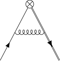
Figure 2: One-loop correction to the vertex function of the bilinear $\phi$.

For the one-loop vertex function (Fig. 2), we use the free quark and gluon propagators in mixed space: position space parallel to $n$ and momentum space for the $d-1$ orthogonal dimensions. We decompose a general vector as $v\equiv v_{n}n+v_{\perp}$, where $v_{n}=n\cdot v$. The gluon propagator takes the form

$$\bar{D}_{\mu\nu}^{AB}(x_{n},p_{\perp})\equiv\int\frac{dp_{n}}{2\pi}e^{ip_{n}x_{n}}D^{AB}_{\mu\nu}(p)=\delta^{AB}\frac{e^{-|x_{n}||p_{\perp}|}}{2|p_{\perp}|}\biggl{[}\\ \delta_{\mu\nu}-\frac{1-\lambda}{2|p_{\perp}|^{2}}\left(|x_{n}||p_{\perp}|p^{*}_{\mu}p^{*}_{\nu}+p_{\perp\mu}p_{\perp\nu}+|p_{\perp}|^{2}n_{\mu}n_{\nu}\right)\biggr{]},$$ (20)

where $p^{*}\equiv p_{\perp}+i\operatorname{sgn}(x_{n})|p_{\perp}|n$. Similarly, for the quark propagator we obtain

$$\bar{S}_{\psi}^{\text{tree}}(x_{n},p_{\perp})\equiv\int\frac{dp_{n}}{2\pi}e^{ip_{n}x_{n}}\frac{-i\not{p}}{p^{2}}=\delta^{ab}e^{-|x_{n}||p_{\perp}|}\frac{-i\not{p}^{*}}{2|p_{\perp}|}.$$ (21)

We write the quantity in Eq. (14), as

$$\Lambda_{\phi}(\xi,p)\equiv S_{\zeta}^{-1}(\xi)G(\xi,p)S_{\psi}^{-1}(p).$$ (22)

This is similar to an amputated vertex function, except that the $\zeta$-leg “amputation” is done in position space rather than the usual momentum space. At one-loop order, this takes the form

$$\Lambda_{\phi}(\xi,p)=1+(ig)^{2}\mu^{4-d}S_{\zeta}^{\text{tree}}(\xi)^{-1}\int_{0}^{\xi}d\xi_{1}\int dx_{n}e^{ix_{n}p_{n}}\int\frac{d^{d-1}k_{\perp}}{(2\pi)^{d-1}}\biggl{[}\\ S_{\zeta}^{\text{tree}}(\xi-\xi_{1})T^{A}n_{\mu}S_{\zeta}^{\text{tree}}(\xi_{1})\bar{S}_{\psi}^{\text{tree}}(-x_{n},p_{\perp}-k_{\perp})T^{B}\gamma_{\nu}\bar{D}^{AB}_{\mu\nu}(\xi_{1}-x_{n},k_{\perp})\biggr{]}.$$ (23)

We simplify the calculation by restricting ourselves to the kinematics $p_{\perp}=0$ and $p_{n}>0$ (i.e. $z=1$), which leads to

$$\frac{1}{12}\operatorname{Tr}\Lambda_{\phi}(\xi,p)=1-g^{2}\mu^{4-d}C_{F}\int_{0}^{\xi}d\xi_{1}\int dx_{n}e^{ix_{n}p_{n}}\int\frac{d^{d-1}k_{\perp}}{(2\pi)^{d-1}}\biggl{[}e^{-|k_{\perp}|(|x_{n}|+|\xi_{1}-x_{n}|)}\\ \times\frac{-1}{4|k_{\perp}|}\bigl{(}\tfrac{1+\lambda}{2}\operatorname{sgn}(x_{n})+\tfrac{1-\lambda}{2}|\xi_{1}-x_{n}||k_{\perp}|[\operatorname{sgn}(x_{n})-\operatorname{sgn}(\xi_{1}-x_{n})]\bigr{)}\biggr{]}.$$ (24)

Eventually, we obtain

$$\frac{1}{12}\Re\operatorname{Tr}\Lambda_{\phi}^{\overline{\text{MS}}}(\xi,p;\mu)=1+\frac{\alpha_{s}C_{F}}{2\pi}\Biggl{(}\lambda\left(1+\log\frac{\mu}{p_{n}}\right)-2\log 2-\frac{1+\lambda}{2}\frac{\sin p_{n}\xi}{p_{n}\xi}-\frac{1-\lambda}{4}(\cos p_{n}\xi-3)\\ +\left[(\lambda-2)\cos\frac{p_{n}\xi}{2}-\frac{1-\lambda}{4}p_{n}\xi\sin\frac{p_{n}\xi}{2}\right]\operatorname{Ci}\left(\frac{p_{n}\xi}{2}\right)+2\operatorname{Ci}(p_{n}\xi)\Biggr{)},$$ (25)

where $\operatorname{Ci}$ is the cosine integral function, $\operatorname{Ci}(z)\equiv-\int_{z}^{\infty}\frac{\cos(t)}{t}dt$.

The $\phi$ conversion factor can be evaluated using $C_{\phi}=\sqrt{C_{\zeta}C_{\psi}}\frac{1}{12}\Re\operatorname{Tr}\Lambda_{\phi}^{\overline{\text{MS}}}$ with the appropriate kinematics. In Landau gauge ($\lambda=0$), we obtain

$$C_{\phi}(y)=1+\frac{\alpha_{s}C_{F}}{2\pi}\biggl{[}\frac{3}{2}\log\frac{y}{4}+\frac{3}{2}\gamma_{E}-2\log 2+\frac{7}{4}-\frac{\cos y}{4}\\ -\left(2\cos\frac{y}{2}-\frac{y}{4}\sin\frac{y}{2}\right)\operatorname{Ci}\left(\frac{y}{2}\right)+2\operatorname{Ci}(y)\biggr{]}+O(\alpha_{s}^{2}).$$ (26)

We also find an anomalous dimension consistent with the leading term obtained first in the auxiliary field theory Craigie and Dorn (1981); Dorn (1986) and later also for the static-light current Voloshin and Shifman (1987); Politzer and Wise (1988a, b); Chetyrkin and Grozin (2003).

To match the auxiliary field mass, one can use the higher-order results from Ref. Chetyrkin and Grozin (2003). Comparing conventions, our $S_{\zeta}$ corresponds to their coordinate-space $i\tilde{S}_{r}$ and our $Z_{\zeta}$ corresponds to their $\tilde{Z}_{Q}^{-1}$. That reference gives

$$\log S_{\zeta}^{\overline{\text{MS}}}(\xi;\mu_{\xi})=f_{\zeta}(\alpha_{\xi}),$$ (27)

where $\mu_{\xi}\equiv\frac{2}{\xi}e^{-\gamma_{E}}$, $\alpha_{\xi}\equiv\alpha_{s}(\mu_{\xi})$, and $f_{\zeta}(x)$ is a series in $x$ given up to $O(x^{3})$. Together with the anomalous dimension $\tilde{\gamma}_{Q}\equiv\frac{d\log\tilde{Z}_{Q}}{d\log\mu}$ and the beta function $\beta\equiv\frac{-1}{2}\frac{d\log\alpha_{s}}{d\log\mu}$, we obtain

$$-\frac{d}{d\xi}\log S_{\zeta}^{\overline{\text{MS}}}(\xi;\mu_{0})=\frac{1}{\xi}\left[\tilde{\gamma}_{Q}(\alpha_{\xi})-2\alpha_{\xi}\beta(\alpha_{\xi})f_{\zeta}^{\prime}(\alpha_{\xi})\right],$$ (28)

which is independent of the scale $\mu_{0}$. Perturbatively, this is limited by $\tilde{\gamma}_{Q}$, which has been computed to order $\alpha_{s}^{3}$ Chetyrkin and Grozin (2003); Melnikov and van Ritbergen (2000).

III Improvement

In the Symanzik approach Symanzik (1983); Lüscher et al. (1996), the lattice theory is described by a continuum effective theory that is an expansion in powers of the lattice spacing, where each term has the same symmetries as the lattice theory. The same is also done for composite operators. The idea of improvement is to add higher dimensional operators in order to tune the parameters of the Symanzik theory such that the leading [e.g. $O(a)$] term in the continuum extrapolation of every correlation function is eliminated.

For the lattice fermion action we take Wilson twisted mass fermions, working in the twisted basis with the fermion doublet $\chi$, although we will also consider chiral fermions. The leading continuum Lagrangian is twisted mass QCD,

$$\mathcal{L}_{\chi}^{(0)}=\bar{\chi}(\not{D}+m_{q}+i\mu_{q}\gamma_{5}\tau^{3})\chi.$$ (29)

At the next order $\mathcal{L}_{\chi}^{(1)}$ contains terms that can be absorbed into the parameters of the leading Lagrangian along with one nontrivial one, the well-known “clover” term Sheikholeslami and Wohlert (1985); Lüscher et al. (1996); Shindler (2008) associated with chiral symmetry breaking. For the auxiliary field in the continuum, we have

$$\mathcal{L}_{\zeta}^{(0)}=\bar{\zeta}(n\cdot D+m)\zeta.$$ (30)

Exact symmetries of the lattice theory include the little group of hypercubic rotations that preserve $n$ and the $U(1)$ charge symmetry for the auxiliary field. There are also several spurionic symmetries Dorn (1986); Shindler (2008); Chen et al. (2019):

1. General hypercubic rotations, together with the rotation of $n$.

2. Parity with respect to the axis $n$, i.e. the negation of the part of space-time vectors orthogonal to $n$, together with the negation of $\mu_{q}$.

3. Time reversal with respect to the axis $n$, together with the negation of $\mu_{q}$ and $n$.

4. Charge conjugation, together with the negation of $n$. Specifically, the auxiliary field transforms as

   $$\zeta_{n}(x)\to\bar{\zeta}_{-n}(x)^{T},\qquad\bar{\zeta}_{n}(x)\to\zeta_{-n}(x)^{T}.$$ (31)

5. Flavor $SU(2)$, together with a rotation of the twisted mass term $\mu_{q}\tau^{3}\to\mu_{q}e^{i\alpha^{a}\tau^{a}}\tau^{3}e^{-i\alpha^{a}\tau^{a}}$.

6. For a chiral fermion action, $SU(2)$ axial transformations together with a rotation of the total mass term $m_{q}+i\mu_{q}\gamma_{5}\tau^{3}$.

Following Kurth and Sommer (2001), the next-order auxiliary field Lagrangian has the form

$$\mathcal{L}_{\zeta}^{(1)}=a(b_{\zeta}m_{q}^{2}+b^{\prime}_{\zeta}\mu_{q}^{2})\bar{\zeta}\zeta,$$ (32)

where $b_{\zeta}$ and $b^{\prime}_{\zeta}$ are $O(g_{0}^{4})$. These terms produce a quark-mass dependence in the auxiliary field mass counterterm. This effect could be significant if charm quarks are included in the lattice action.

III.1 Local bilinear operator

To simplify the study of improvement, we consider a bilinear defined in the twisted basis, $\phi=\bar{\zeta}\chi$. The operator $\not{n}\phi$ transforms in the same way under all of the above symmetries except for $SU(2)$ axial. Therefore at leading order the renormalized operator is given by

$$\phi_{R}=Z_{\phi}(\phi+r_{\text{mix}}\not{n}\phi),$$ (33)

where $r_{\text{mix}}=0$ for a chiral action.

For the $O(a)$ contributions, we follow the study of the static-light axial current in Ref. Kurth and Sommer (2001). However, because of the equation of motion $(\not{D}+m_{q}+i\mu_{q}\tau_{3}\gamma_{5})\chi=0$, there is some freedom in defining the on-shell improvement terms. In particular, we could use a derivative orthogonal to $n$, $\not{D}_{\perp}=(\delta_{\mu\nu}-n_{\mu}n_{\nu})\gamma_{\mu}D_{\nu}$ as in Ref. Kurth and Sommer (2001). However, for the case of quasi-PDFs it may be better to use a derivative along $n$: this would keep the improved operator from extending across more than one time slice and could potentially allow $O(a)$ improvement to be applied to existing data. Furthermore, we use the equations of motion for $\zeta$ to write $\bar{\zeta}n\cdot D\chi=n\cdot\partial(\bar{\zeta}\chi)$. At $O(a)$, we obtain the improved operator,

$$\phi_{R,I} =Z_{\phi}(\phi+r_{\text{mix}}\not{n}\phi+a\phi_{1,m}+a\phi_{1,D}),$$ (34)

$$\phi_{1,m} =\left[(b_{\phi}+\bar{b}_{\phi}\not{n})\not{n}m_{q}+(b^{\prime}_{\phi}+\bar{b}^{\prime}_{\phi}\not{n})\not{n}i\mu_{q}\tau^{3}\gamma_{5}\right]\phi,$$

$$\phi_{1,D} =(c_{\phi}+\bar{c}_{\phi}\not{n})n\cdot\partial\phi.$$

For a chiral action, $\bar{b}_{\phi}$, $\bar{b}^{\prime}_{\phi}$, and $\bar{c}_{\phi}$ vanish and $b_{\phi}=b^{\prime}_{\phi}$ but there still exist terms at $O(a)$ that can not be excluded. Note that this expression assumes only a single doublet of fermions is present; for additional nondegenerate fermions there can be additional terms involving, for example, the trace of the mass matrix, as discussed in Ref. Bhattacharya et al. (2006). For $\bar{\phi}=\bar{\chi}\zeta$, we apply charge conjugation and then relabel $n\to-n$ to obtain

$$\bar{\phi}_{R,I} =Z_{\phi}(\bar{\phi}+r_{\text{mix}}\bar{\phi}\not{n}+a\bar{\phi}_{1,m}+a\bar{\phi}_{1,D})$$ (35)

$$\bar{\phi}_{1,m} =\bar{\phi}\left[m_{q}\not{n}(b_{\phi}+\bar{b}_{\phi}\not{n})+i\mu_{q}\tau^{3}\gamma_{5}\not{n}(b^{\prime}_{\phi}+\bar{b}^{\prime}_{\phi}\not{n})\right],$$

$$\bar{\phi}_{1,D} =-n\cdot\partial\bar{\phi}(c_{\phi}+\bar{c}_{\phi}\not{n}).$$

One further consideration is if the lattice gauge links used for the Wilson line are obtained using an anisotropic smearing, which breaks some of the hypercubic rotations and allows additional contributions. This is used in calculations by ETMC, where (for $n$ in a spatial direction) the gauge links are smeared only in spatial directions and not in time Alexandrou et al. (2019a). There is again some freedom in defining the on-shell improvement due to the equations of motion for $\chi$. If smearing is not performed in the $t$ direction, then one possible form for the additional term is $(c^{\prime}_{\phi}+\bar{c}^{\prime}_{\phi}\not{n})\gamma_{t}\bar{\zeta}D_{t}\chi$. We will not explicitly consider this anisotropic case below, but the generalization is straightforward.

III.2 Operator for quasi-PDFs

Using the fermion doublet $\chi$, we consider the operator

$$\mathcal{O}_{\Gamma\tau}(\xi)=\bar{\chi}(\xi n)\Gamma\tau W(\xi n,0)\chi(0)=\left\langle\bar{\phi}(\xi n)\Gamma\tau\phi(0)\right\rangle_{\zeta},$$ (36)

inserted at zero momentum, where $\Gamma$ is a generic spin matrix and $\tau$ is a generic flavor matrix. The improved, renormalized operator is given (for $\xi>0$) by

$$\begin{gathered}\begin{aligned} \mathcal{O}^{R,I}_{\Gamma\tau}(\xi)&=\langle\bar{\phi}_{R,I}(\xi n)\Gamma\tau\phi_{R,I}(0)\rangle_{\zeta}\\ &=Z_{\phi}^{2}e^{-m\xi}\biggl{(}\bar{\chi}(\xi n)XW(\xi n,0)\chi(0)\\ &\qquad\qquad\quad+a\left.\frac{\partial}{\partial\eta}\bigl{[}\bar{\chi}(\xi n)W(\xi n,\eta n)(1+r_{\text{mix}}\not{n})\Gamma\tau(c_{\phi}+\bar{c}_{\phi}\not{n})\chi(\eta n)\bigr{]}\right|_{\eta=0}\\ &\qquad\qquad\quad-a\frac{\partial}{\partial\xi}\bigl{[}\bar{\chi}(\xi n)W(\xi n,0)(c_{\phi}+\bar{c}_{\phi}\not{n})\Gamma\tau(1+r_{\text{mix}}\not{n})\chi(0)\bigr{]}\biggr{)}+O(a^{2}),\end{aligned}\\ \begin{aligned} X&=\Gamma\tau+r_{\text{mix}}\{\Gamma,\not{n}\}\tau+r_{\text{mix}}^{2}\not{n}\Gamma\not{n}\tau\\ &\quad+am_{q}\bigl{(}2\bar{b}_{\phi}\Gamma\tau+(b_{\phi}+r_{\text{mix}}\bar{b}_{\phi})\{\Gamma,\not{n}\}\tau+2b_{\phi}r_{\text{mix}}\not{n}\Gamma\not{n}\tau\bigr{)}\\ &\quad+ia\mu_{q}\bigl{(}b^{\prime}_{\phi}[\Gamma\tau,\not{n}\gamma_{5}\tau^{3}]+\bar{b}^{\prime}_{\phi}\{\Gamma\tau,\gamma_{5}\tau^{3}\}+r_{\text{mix}}(\bar{b}^{\prime}_{\phi}[\not{n}\Gamma\not{n}\tau,\not{n}\gamma_{5}\tau^{3}]+b^{\prime}_{\phi}\{\not{n}\Gamma\not{n}\tau,\gamma_{5}\tau^{3}\})\bigr{)}.\end{aligned}\end{gathered}$$ (37)

Since the operator is inserted at zero momentum, we can add a total derivative to finally obtain

$$\begin{gathered}\mathcal{O}^{R,I}_{\Gamma\tau}(\xi)=Z_{\phi}^{2}e^{-m\xi}\left[\mathcal{O}_{X}(\xi)-a\frac{\partial}{\partial\xi}\mathcal{O}_{\Gamma_{D}\tau}(\xi)\right]+O(a^{2})+\text{total derivative},\\ \Gamma_{D}=2c_{\phi}\Gamma+(\bar{c}_{\phi}+c_{\phi}r_{\text{mix}})\{\Gamma,\not{n}\}+2c_{\phi}r_{\text{mix}}\not{n}\Gamma\not{n}.\end{gathered}$$ (38)

For specific choices of $\Gamma$ and $\tau$, this expression simplifies. Calculations of quasi-PDFs are typically done with a flavor diagonal operator where $\tau$ commutes with $\tau^{3}$. It has become standard to compute unpolarized quasi-PDFs using $\Gamma=\gamma_{\nu}$ with $\nu$ satisfying $n_{\nu}=0$ and helicity quasi-PDFs using $\Gamma=\not{n}\gamma_{5}$. In both of these cases, $\not{n}\Gamma\not{n}=-\Gamma$ and all of the (anti)commutators vanish, so that the improved operator becomes

$$\text{(no-mixing case)}\quad\mathcal{O}^{R,I}_{\Gamma\tau}(\xi)=Z_{\phi}^{2}e^{-m\xi}\left[1-r_{\text{mix}}^{2}+2am_{q}(\bar{b}_{\phi}-b_{\phi}r_{\text{mix}})-2(c_{\phi}-\bar{c}_{\phi}r_{\text{mix}})a\frac{\partial}{\partial\xi}\right]\mathcal{O}_{\Gamma\tau}(\xi),$$ (39)

i.e. only the derivative operator (and no other mixing) contributes at $O(a)$ and the only nontrivial effect of chiral symmetry breaking is the dependence on $am_{q}$. Transversity quasi-PDFs are computed using an operator that has $\Gamma=\not{n}\gamma_{\nu}$ in the physical basis. If $\mu_{q}=0$, then Eq. (39) again applies. On the other hand, when using twisted mass fermions at maximal twist we must consider the corresponding twisted-basis operator. For the case of a flavor diagonal transversity operator, the twisted-basis operator has $\Gamma=i\not{n}\gamma_{\nu}\gamma_{5}$ and suffers from equal-dimensional mixing because $\{\Gamma,\not{n}\}=2i\gamma_{\nu}\gamma_{5}$. Using a flavor-changing transversity operator would be advantageous: it appears the same in the physical and twisted bases and the form of the improved operator is given by Eq. (39).

III.2.1 Maximal twist

In calculations done using Wilson twisted mass fermions, many correlators benefit from automatic $O(a)$ improvement Frezzotti and Rossi (2004); Shindler (2008). This means that when tuned to maximal twist ($m_{q}=0$), the $O(a)$ contributions to those correlation functions vanish and there is no need to explicitly tune the improvement coefficients. For the case considered here, the arguments behind automatic improvement do not eliminate all of the $O(a)$ contributions, but they do eliminate the contributions that vanish for chiral fermion actions.

We start by working at $O(a^{0})$ and examining the equal-dimensional mixing. To simplify the expressions, assume $\not{n}\Gamma\not{n}=G_{\Gamma}\Gamma$, where $G_{\Gamma}=\pm 1$. We then write

$$\mathcal{O}_{\Gamma\tau}^{R}(\xi) =Z_{\phi}^{2}e^{-m\xi}\left[(1+G_{\Gamma}r_{\text{mix}}^{2})\mathcal{O}_{\Gamma\tau}(\xi)+r_{\text{mix}}\mathcal{O}_{\{\Gamma,\not{n}\}\tau}(\xi)\right]+O(a),$$ (40)

$$\mathcal{O}_{\{\Gamma,\not{n}\}\tau}^{R}(\xi) =Z_{\phi}^{2}e^{-m\xi}\left[(1+r_{\text{mix}}^{2})\mathcal{O}_{\{\Gamma,\not{n}\}\tau}(\xi)+2(1+G_{\Gamma})r_{\text{mix}}\mathcal{O}_{\Gamma\tau}(\xi)\right]+O(a).$$ (41)

Using these two equations we can eliminate $\mathcal{O}_{\{\Gamma,\not{n}\}\tau}$ and obtain

$$\mathcal{O}_{\Gamma\tau}(\xi)=\frac{e^{m\xi}}{\tilde{Z}^{2}_{\phi,G_{\Gamma}}}\left[\mathcal{O}_{\Gamma\tau}^{R}(\xi)-\frac{r_{\text{mix}}}{1+r_{\text{mix}}^{2}}\mathcal{O}_{\{\Gamma,\not{n}\}\tau}^{R}(\xi)\right]+O(a),$$ (42)

where $\tilde{Z}^{2}_{\phi,G}=Z_{\phi}^{2}(1-r_{\text{mix}}^{2})(1-Gr_{\text{mix}}^{2})/(1+r_{\text{mix}}^{2})$.

We now consider the transformations

$$\mathcal{R}_{5}^{1,2}:\begin{cases}\chi\to i\gamma_{5}\tau^{1,2}\chi\\ \bar{\chi}\to\bar{\chi}i\gamma_{5}\tau^{1,2}\end{cases},$$ (43)

which are chiral symmetries of continuum twisted mass QCD at maximal twist. Clearly, if $\mathcal{O}_{\Gamma\tau}\to R\mathcal{O}_{\Gamma\tau}$ ($R=\pm 1$) under one of these transformations, then $\mathcal{O}_{\{\Gamma,\not{n}\}\tau}\to-R\mathcal{O}_{\{\Gamma,\not{n}\}\tau}$. Now, consider a correlation function involving some hadronic interpolators and $\mathcal{O}_{\Gamma\tau}$ that is invariant under $\mathcal{R}_{5}^{1,2}$. In the continuum, the corresponding correlation function with $\mathcal{O}_{\{\Gamma,\not{n}\}\tau}$ will vanish because it is odd under $\mathcal{R}_{5}^{1,2}$. On the lattice, for the renormalized operator $\mathcal{O}_{\{\Gamma,\not{n}\}\tau}^{R}$ the result must therefore be $O(a)$ and this term can be neglected in Eq. (42). Effectively, one can use $\mathcal{O}_{\Gamma\tau}^{R}(\xi)=\tilde{Z}^{2}_{\phi,G_{\Gamma}}e^{-m\xi}\mathcal{O}_{\Gamma\tau}(\xi)+O(a)$. This justifies the calculation in Refs. Alexandrou et al. (2018b, 2019a), where equal-dimensional mixing for the transversity operator was not explicitly treated.

Now, we move on to the $O(a)$ contributions. Specifically, we take the correlation function of the product of $\mathcal{O}_{\Gamma}$ inserted at zero momentum with a renormalized $O(a)$-improved multilocal field $\Phi$. The Symanzik expansion of the lattice correlator is given by

$$\bigl{\langle}\Phi\mathcal{O}_{\Gamma\tau}(\xi)\bigr{\rangle} =\frac{e^{m\xi}}{\tilde{Z}^{2}_{\phi,G_{\Gamma}}}\left\langle\Phi\left[\mathcal{O}_{\Gamma\tau}^{R}(\xi)-\frac{r_{\text{mix}}}{1+r_{\text{mix}}^{2}}\mathcal{O}_{\{\Gamma,\not{n}\}\tau}^{R}(\xi)\right]\right\rangle_{0}$$ (44)

$$\quad-\frac{e^{m\xi}}{\tilde{Z}^{2}_{\phi,G_{\Gamma}}}a\left\langle\Phi\left[\mathcal{O}_{\Gamma\tau}^{R}(\xi)-\frac{r_{\text{mix}}}{1+r_{\text{mix}}^{2}}\mathcal{O}_{\{\Gamma,\not{n}\}\tau}^{R}(\xi)\right]\int d^{4}x\mathcal{L}_{\chi}^{(1)}(x)\right\rangle_{0}$$

$$\quad+a\left\langle\Phi\mathcal{O}_{\Gamma\tau}^{(1)}(\xi)\right\rangle_{0}+O(a^{2}),$$

where $\langle\cdots\rangle_{0}$ is evaluated in the continuum theory and $\mathcal{O}_{\Gamma\tau}^{(1)}(\xi)$ contains the $O(a)$ terms that appear in Eq. (38). Assuming $\Phi\mathcal{O}_{\Gamma\tau}$ is invariant under $\mathcal{R}_{5}^{1,2}$ and $m_{q}=0$, many of the terms vanish and we get

$$\tilde{Z}^{2}_{\phi,G_{\Gamma}}e^{-m\xi}\bigl{\langle}\Phi\mathcal{O}_{\Gamma\tau}(\xi)\bigr{\rangle} =\left\langle\Phi\mathcal{O}_{\Gamma\tau}^{R}(\xi)\right\rangle_{0}+\frac{r_{\text{mix}}}{1+r_{\text{mix}}^{2}}a\left\langle\Phi\mathcal{O}_{\{\Gamma,\not{n}\}\tau}^{R}(\xi)\int d^{4}x\mathcal{L}_{\chi}^{(1)}(x)\right\rangle_{0}$$ (45)

$$\quad+a\left\langle\Phi\left[c_{1,G_{\Gamma}}i\mu_{q}\mathcal{O}^{R}_{[\Gamma\tau,\not{n}\gamma_{5}\tau^{3}]}(\xi)+c_{2,G_{\Gamma}}\frac{\partial}{\partial\xi}\mathcal{O}^{R}_{\Gamma\tau}(\xi)\right]\right\rangle_{0},$$

for some prefactors $c_{1,\pm}$ and $c_{2,\pm}$. If the fermion action is $O(a)$ improved by including a clover term, then $\mathcal{L}^{(1)}_{\chi}$ vanishes and one can effectively obtain $O(a)$ improvement by using

$$\begin{gathered}\mathcal{O}_{\Gamma\tau}^{R,I}(\xi)=\tilde{Z}^{2}_{\phi,G_{\Gamma}}e^{-m\xi}\left[\mathcal{O}_{\tilde{X}}(\xi)-\tilde{c}_{\phi,G_{\Gamma}}a\frac{\partial}{\partial\xi}\mathcal{O}_{\Gamma\tau}(\xi)\right],\\ \tilde{X}=\Gamma\tau-i\tilde{b}^{\prime}_{\phi,G_{\Gamma}}a\mu_{q}[\Gamma\tau,\not{n}\gamma_{5}\tau^{3}],\end{gathered}$$ (46)

where six parameters remain: $\tilde{Z}_{\phi,+}$, $\tilde{b}^{\prime}_{\phi,+}$, $\tilde{c}_{\phi,+}$, $\tilde{Z}_{\phi,-}$, $\tilde{b}^{\prime}_{\phi,-}$, and $\tilde{c}_{\phi,-}$. Usually the operator will have a definite $G_{\Gamma}$, so that only half of the parameters can contribute, and for many operators the commutator vanishes so that the term proportional to $a\mu_{q}$ does not contribute. On the other hand, if the fermion action is not $O(a)$ improved, then the second term in Eq. (45) can be eliminated either by explicitly treating the $O(a^{0})$ mixing or by choosing an operator such that $\{\Gamma,\not{n}\}=0$.

The term involving the $O(a)$ part of the fermion action survives in Eq. (45) because the connection between dimensional counting and breaking of chiral symmetry, which underlies the usual arguments for automatic improvement, is broken by the equal-dimensional mixing with $\mathcal{O}_{\{\Gamma,\not{n}\}\tau}$. This leads to another potential worry: if $\Phi$ is not $O(a)$ improved, as is typically the case for interpolating operators, then an additional nonvanishing term of the form $a\langle\Phi^{(1)}\mathcal{O}^{R}_{\{\Gamma,\not{n}\}\tau}\rangle_{0}$ can appear in Eq. (45). However, although this is an $O(a)$ contribution in the correlation function, it can be argued that it will not contribute to the ground-state hadronic matrix element determined at large Euclidean time separations, since the latter is independent of the interpolating operator. To see this, consider a correlation function using local hadron interpolators that have been explicitly $O(a)$ improved. In this case, the Symanzik expansion is given by Eq. (45) and the $O(a)$ terms can be eliminated by including a clover term in the fermion action and tuning the improvement parameters in Eq. (46). Once the correlation function is free of $O(a)$ effects, then, following the arguments in Section 3.2 of Ref. Frezzotti and Rossi (2004), we find that the matrix element obtained at large time separations will be free of $O(a)$ effects. As the same ground-state matrix element can be obtained using any interpolating operator, the $O(a)$-improved ground-state matrix element can thus be obtained from the large-time-separation limit of a correlation function even if the interpolator is not $O(a)$ improved.

III.3 Determining improvement coefficients

In principle, parameters associated with breaking of chiral symmetry ($r_{\text{mix}}$, $\bar{b}_{\phi}$, $\bar{b}^{\prime}_{\phi}$, $b_{\phi}-b^{\prime}_{\phi}$, and $\bar{c}_{\phi}$) can be determined using improvement conditions derived from chiral Ward identities Lüscher et al. (1996); this approach was used for nonperturbative determinations of closely-related parameters in the static quark theory in Refs. Aoki et al. (2000); Hashimoto et al. (2002); Palombi (2008). For the remaining improvement coefficients $b_{\phi}$ and $c_{\phi}$, the situation is more difficult as there is no simple continuum physics condition to match onto: one would have to numerically study the continuum extrapolation of suitably chosen observables and tune the parameters to eliminate the linear dependence on $a$. Alternatively, the parameters could be computed in lattice perturbation theory, which has been done for the static quark theory using a few different lattice actions Morningstar and Shigemitsu (1998); Ishikawa et al. (2000); Kurth and Sommer (2001); Della Morte et al. (2005); Palombi (2008); Grimbach et al. (2008); Ishikawa et al. (2011).

IV General link paths

In this section we generalize our use of the auxiliary field approach on the lattice to describe paths that have corners and paths that are not along a lattice axis. In part, this will serve to understand under which circumstances the assumption made in Refs. Hägler et al. (2009); Musch et al. (2011, 2012); Engelhardt et al. (2016) (and studied empirically in Ref. Yoon et al. (2017)), that the continuum renormalization pattern Dorn (1986) applies to lattice calculations, is valid.

IV.1 Piecewise straight paths

Nonlocal operators with link paths that are not straight are also used for hadron structure; in particular, staple-shaped gauge connections have been used for studying transverse momentum-dependent (TMD) PDFs. If the path is made from a finite number of segments, each of which is a Wilson line propagating along a lattice axis, then it is straightforward to accommodate the nonlocal operator in the lattice auxiliary field framework. An auxiliary field $\zeta_{n}$ must be introduced for each segment, where $n$ is the corresponding direction. In addition to suitable bilinears $\phi_{n_{i}}\equiv\bar{\zeta}_{n_{i}}\psi$ and $\bar{\phi}_{n_{f}}$ for the endpoints, one must also introduce cusp operators Polyakov (1980); Craigie and Dorn (1981) $C_{n^{\prime},n}=\bar{\zeta}_{n^{\prime}}\zeta_{n}$ for each transition between segments.

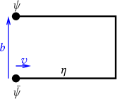
Figure 3: Staple-shaped operator.

To be concrete, consider the TMD operator with quark fields separated by the four-vector $b$ and the staple of height $\eta$ in the direction of the unit vector $v$ that is orthogonal to $b$ (see Fig. 3):

$$\mathcal{O}^{\text{TMD}}_{\Gamma}=\bar{\psi}(0)\Gamma W(0,\eta v)W(\eta v,\eta v+b)W(\eta v+b,b)\psi(b).$$ (47)

We introduce the auxiliary fields $\zeta_{v}$, $\zeta_{-v}$, and $\zeta_{-\hat{b}}$, and obtain

$$\mathcal{O}^{\text{TMD}}_{\Gamma}=\left\langle\bar{\phi}_{-v}(0)\Gamma C_{-v,-\hat{b}}(\eta v)C_{-\hat{b},v}(\eta v+b)\phi_{v}(b)\right\rangle_{\zeta}.$$ (48)

In addition to renormalizing the action for the auxiliary fields and the bilinears $\phi$, the cusp operators must also be renormalized. The latter are not expected to mix. However, since the operators $\phi_{v}$ and $\bar{\phi}_{-v}$ connect to auxiliary fields propagating in opposite directions, the mixing pattern allowed by chiral symmetry breaking is different from the straight-line operators used for quasi-PDFs: $\mathcal{O}^{\text{TMD}}_{\Gamma}$ can mix with $\mathcal{O}^{\text{TMD}}_{[\Gamma,\not{v}]}$. This was pointed out by one of us in Ref. Green (2018) and later confirmed at one-loop order in lattice perturbation theory Constantinou et al. (2019). The latter calculation also found that more generally, the pattern of mixing depends only on the direction with which the Wilson lines hit the quark fields, which is consistent with the prediction of the auxiliary field approach. We note that a numerical study of nonperturbative renormalization of staple-shaped operators was recently done in Ref. Shanahan et al. (2019).

A RI-xMOM renormalization condition for cusp operators is straightforward to formulate. This requires the position-space Green’s function for the cusp operator,

$$G_{C}(\xi^{\prime},\xi)\equiv\langle\zeta_{n^{\prime}}(\xi^{\prime}n^{\prime})C_{n^{\prime},n}(0)\bar{\zeta}(-\xi n)\rangle_{\text{QCD}+\zeta}=\langle W(\xi^{\prime}n^{\prime},0)W(0,-\xi n)\rangle_{\text{QCD}}.$$ (49)

Performing a position-space “amputation”, a possible condition is

$$\frac{1}{3}\frac{Z_{C}}{Z_{\zeta}}\operatorname{Tr}\left[S_{\zeta_{n^{\prime}}}^{-1}(\xi^{\prime})G_{C}(\xi^{\prime},\xi)S_{\zeta_{n}}^{-1}(\xi)\right]=1,$$ (50)

when $\xi^{\prime}=\xi=\mu^{-1}$.

IV.2 Off-axis paths

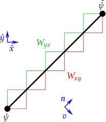
Figure 4: Off-axis operator with two different discretizations of the Wilson line.

It is possible to somewhat relax the constraint that $n$ points along a lattice axis. For example, let $n=\frac{1}{\sqrt{2}}(\hat{x}+\hat{y})$. On the lattice, one definition of the straight-line operator is Musch et al. (2011)

$$\mathcal{O}_{\Gamma}^{\text{lat}}(0,\xi,n)\equiv\bar{\psi}(\xi n)\Gamma\frac{1}{2}\left[W_{xy}(\xi n,0)+W_{yx}(\xi n,0)\right]\psi(0),$$ (51)

where $W_{xy}$ is formed from the zigzag product of gauge links alternating between the $x$ and $y$ directions and vice-versa for $W_{yx}$ (see Fig. 4). This average is necessary so that the operator has a simple transformation under $n$-parity. These zigzag Wilson lines can be obtained as propagators of auxiliary fields $\zeta_{xy}$ and $\zeta_{yx}$ that are defined using two-link covariant derivatives along the $n$ direction, e.g.:

$$\nabla_{xy}f(x)=\frac{1}{\sqrt{2}a}\left[f(x)-U_{y}^{\dagger}(x-a\hat{y})U_{x}^{\dagger}(x-a(\hat{x}+\hat{y}))f(x-a(\hat{x}+\hat{y}))\right].$$ (52)

Because of rotational symmetry breaking on the lattice, the mass counterterm $m_{xy}=m_{yx}$ will in general be different from the on-axis case. The quark bilinear takes the form

$$\mathcal{O}_{\Gamma}^{\text{lat}}(0,\xi,n)=\left\langle\frac{1}{2}\left[\bar{\phi}_{xy}(\xi n)\Gamma\phi_{xy}(0)+\bar{\phi}_{yx}(\xi n)\Gamma\phi_{yx}(0)\right]\right\rangle_{\zeta},$$ (53)

where $\phi_{xy}=\bar{\zeta}_{xy}\psi$, etc. Defining $\varphi_{\pm}\equiv\frac{1}{\sqrt{2}}(\phi_{xy}\pm\phi_{yx})$, this can be rewritten as

$$\mathcal{O}_{\Gamma}^{\text{lat}}(0,\xi,n)=\left\langle\bar{\varphi}_{\pm}(\xi n)\Gamma\varphi_{\pm}(0)\right\rangle_{\zeta},$$ (54)

where the additional cross terms involving e.g. $\langle\zeta_{xy}\bar{\zeta}_{yx}\rangle$ vanish. Under $n$-parity, $\varphi_{\pm}\to\pm\not{n}\varphi_{\pm}$.

We find that additional mixing can occur. Defining $v=\frac{1}{\sqrt{2}}(\hat{x}-\hat{y})$, $\varphi_{+}$ mixes with $\not{n}\varphi_{+}$, $\not{v}\varphi_{-}$, and $\not{n}\not{v}\varphi_{-}$, the last of which is a chiral-even mixing. This leads to correlation functions of the form $\langle\bar{\varphi}_{+}\varphi_{-}\rangle$, which contain a difference of Wilson lines $W_{xy}-W_{yx}$. One expects that this difference will vanish in the continuum limit. This expectation can be justified in the auxiliary field approach: in the continuum, there is an $SU(2)$ flavor symmetry relating $\zeta_{xy}$ and $\zeta_{yx}$. It is broken in the next order of the Symanzik expansion, where a term of the form $a\bar{\zeta}_{xy}G_{\mu\nu}n_{\mu}v_{\nu}\zeta_{xy}-a\bar{\zeta}_{yx}G_{\mu\nu}n_{\mu}v_{\nu}\zeta_{yx}$ can appear in the Lagrangian; this implies that $\langle\bar{\varphi}_{+}\varphi_{-}\rangle$ is $O(a)$. Therefore, even though the mixing between $\varphi_{+}$ and operators containing $\varphi_{-}$ is equal-dimensional, the most serious new mixing effect in correlation functions is suppressed by at least $O(a)$. The remaining effect is that even when using a chiral fermion action, renormalization will be different for operators where $\not{v}\not{n}\Gamma\not{n}\not{v}$ is equal to $+\Gamma$ and those where it equals $-\Gamma$.

An alternative definition is to average the paths locally. Taking the average of the two local link paths,

$$U_{\text{avg}}(x)\equiv\frac{1}{2}\left[U_{x}(x)U_{y}(x+a\hat{x})+U_{y}(x)U_{x}(a+a\hat{y})\right],$$ (55)

the lattice action for $\zeta_{\text{avg}}$ is defined using the covariant derivative

$$\nabla_{\text{avg}}f(x)=\frac{1}{\sqrt{2}a}\left[f(x)-U_{\text{avg}}^{\dagger}(x-a(\hat{x}+\hat{y}))f(x-a(\hat{x}+\hat{y}))\right].$$ (56)

Again, the mass counterterm will in general be different from the previous case. Then, using the bilinear $\phi_{\text{avg}}=\bar{\zeta}_{\text{avg}}\psi$, the bilocal operator $\langle\bar{\phi}_{\text{avg}}(\xi n)\Gamma\phi_{\text{avg}}(0)\rangle_{\zeta}$ effectively averages over $2^{N}$ link paths, where $\xi=\sqrt{2}Na$. In this case, the pattern of equal-dimensional mixing is the same as the on-axis case.

V Conclusions

The auxiliary field approach is an invaluable tool for understanding the renormalization and improvement of Wilson-line operators on the lattice. Generically, these nonlocal operators can be represented using local operators in an extended theory involving auxiliary fields. We have shown how this can be done for a variety of operators, beyond the simplest ones involving straight on-axis link paths used for quasi-PDF studies.

Using the Symanzik expansion, we were able to study discretization effects and the form of the improved operators. As foreseen in Ref. Green et al. (2018), we find that the leading effects are linear in $a$ even if chiral symmetry is preserved on the lattice. Likewise, we find that working at maximal twist does not automatically eliminate the effects linear in $a$, but it can remove some of the contributions and it can produce some simplification by reducing the number of improvement coefficients. Our analysis provides a general framework for the $O(a)$ improvement of nonlocal operators used in the quasi-PDF approach for computing PDFs on the lattice.

In order to apply this improvement to a lattice calculation of quasi-PDFs, the relevant coefficients for the choice of lattice action must be determined. For some actions, many of these are already known from lattice perturbation theory calculations done for the static quark theory. There are plans to determine the coefficients for actions used by ETMC Constantinou , and we intend to study the effect of improvement on the approach to the continuum limit. It will be important to establish that discretization effects in quasi-PDF calculations can be controlled.

Appendix A Relation to static quark theory

The static quark theory Eichten and Hill (1990); Sommer (2010) is defined using a spinor $Q$ that satisfies $Q=P_{+}Q$, where $P_{\pm}=(1\pm\gamma_{0})/2$. Its two spin degrees of freedom do not couple in its action, and its propagator is the same as the $\zeta$-field propagator with $n=\hat{t}$, multiplied by $P_{+}$. This means that, after accounting for the projector, the static quark and auxiliary field theories can be identified with each other. It will be convenient to define the projected bilinears $\phi^{\pm}=\frac{1}{2}(1\pm\not{n})\phi$, where the projectors become $P_{\pm}$ when $n=\hat{t}$. In our approach, neglecting a twisted mass term, the renormalized $O(a)$-improved operators take the form

$$\phi^{\pm}_{R,I}=Z_{\phi}^{\pm}\left(1\pm b_{\phi}^{\pm}am_{q}+c_{\phi}^{\pm}an\cdot\partial\right)\phi^{\pm},$$ (57)

where $Z_{\phi}^{\pm}=Z_{\phi}(1\pm r_{\text{mix}})$, $b_{\phi}^{\pm}=(b_{\phi}\pm\bar{b}_{\phi})/(1\pm r_{\text{mix}})$, and $c_{\phi}^{\pm}=(c_{\phi}\pm\bar{c}_{\phi})/(1\pm r_{\text{mix}})$.

In Ref. Kurth and Sommer (2001), the time components of the static-light axial and vector currents are defined as

$$A_{0}^{\text{stat}} \equiv\bar{\psi}\gamma_{0}\gamma_{5}Q=-\bar{\psi}P_{-}\gamma_{5}Q,$$ (58)

$$V_{0}^{\text{stat}} \equiv\bar{\psi}\gamma_{0}Q=\bar{\psi}P_{+}Q.$$ (59)

By identifying which projector is contracted with $\bar{\psi}$, this lets us make the identifications

$$A_{0}^{\text{stat}}\to-\bar{\phi}^{-}\gamma_{5},\qquad V_{0}^{\text{stat}}\to\bar{\phi}^{+},$$ (60)

and the corresponding renormalization factors can be equated: $Z_{A}^{\text{stat}}=Z_{\phi}^{-}$ and $Z_{V}^{\text{stat}}=Z_{\phi}^{+}$. For the static-light axial current, Ref. Kurth and Sommer (2001) identifies four possible $O(a)$ improvement operators:

$$(\delta A_{0}^{\text{stat}})_{1} \equiv\bar{\psi}\overset{\leftarrow}{D}_{j}\gamma_{j}\gamma_{5}Q=\bar{\psi}\overset{\leftarrow}{\not{D}}_{\perp}P_{-}\gamma_{5}Q,$$ (61)

$$(\delta A_{0}^{\text{stat}})_{2} \equiv\bar{\psi}\gamma_{5}D_{0}Q=\bar{\psi}P_{-}\gamma_{5}D_{0}Q,$$ (62)

$$(\delta A_{0}^{\text{stat}})_{3} \equiv\bar{\psi}\overset{\leftarrow}{D}_{0}\gamma_{5}Q=-\bar{\psi}\overset{\leftarrow}{D}_{0}\gamma_{0}P_{-}\gamma_{5}Q,$$ (63)

$$(\delta A_{0}^{\text{stat}})_{4} \equiv m_{q}\bar{\psi}\gamma_{0}\gamma_{5}Q=-m_{q}\bar{\psi}P_{-}\gamma_{5}Q.$$ (64)

At leading order, the equations of motion for $Q$ give $(\delta A_{0}^{\text{stat}})_{2}=0$ and those for $\psi$ give $(\delta A_{0}^{\text{stat}})_{1}-(\delta A_{0}^{\text{stat}})_{3}+(\delta A_{0}^{\text{stat}})_{4}=0$; these are used to eliminate $(\delta A_{0}^{\text{stat}})_{2,3}$. The improved, renormalized operator is then given by

$$(A_{R}^{\text{stat}})_{0}=Z_{A}^{\text{stat}}(1+b_{A}^{\text{stat}}am_{q})(A_{I}^{\text{stat}})_{0},\quad(A_{I}^{\text{stat}})_{0}=A_{0}^{\text{stat}}+ac_{A}^{\text{stat}}(\delta A_{0}^{\text{stat}})_{1}.$$ (65)

We can make the identification

$$(\delta A_{0}^{\text{stat}})_{2}+(\delta A_{0}^{\text{stat}})_{3}=\partial_{0}\left(\bar{\psi}P_{-}\gamma_{5}Q\right)\to n\cdot\partial\bar{\phi}^{-}\gamma_{5}.$$ (66)

To relate Eq. (57) with Eq. (65), we need to use the equations of motion to eliminate $(\delta A_{0}^{\text{stat}})_{1}$ and insert $(\delta A_{0}^{\text{stat}})_{2}$. Our identification allows us to equate the improvement coefficients at leading order: $b_{\phi}^{-}=c_{A}^{\text{stat}}-b_{A}^{\text{stat}}$ and $c_{\phi}^{-}=c_{A}^{\text{stat}}$. Likewise, Ref. Kurth and Sommer (2001) gives the improved, renormalized vector current as

$$(V^{\text{stat}}_{R})_{0}=Z_{V}^{\text{stat}}\left(1+b_{V}^{\text{stat}}\right)\left(V_{0}^{\text{stat}}+ac_{V}^{\text{stat}}\bar{\psi}\overset{\leftarrow}{D}_{j}\gamma_{j}Q\right),$$ (67)

and by again using the equations of motion we obtain at leading order $b_{\phi}^{+}=c_{V}^{\text{stat}}+b_{V}^{\text{stat}}$ and $c_{\phi}^{+}=c_{V}^{\text{stat}}$. For a chiral action, our identification leads to $Z_{A}^{\text{stat}}=Z_{V}^{\text{stat}}$, $c_{A}^{\text{stat}}=c_{V}^{\text{stat}}$, and $b_{A}^{\text{stat}}=-b_{V}^{\text{stat}}$, consistent with Ref. Ishikawa et al. (2000).

Appendix B Comparison with whole-operator approach

In Ref. Chen et al. (2019), the symmetry properties of dimension-three operators of type $\mathcal{O}_{\Gamma}(\xi)$ and similar dimension-four nonlocal operators were studied in order to understand mixing and $O(a)$ effects. We find the same pattern of mixing with three-dimensional operators and four-dimensional operators proportional to $m_{q}$. However, in general it is much less constraining to consider the operator as a whole rather than using the auxiliary field approach to represent it using two local operators. This leads to the following differences:

1. The auxiliary field approach implies that for a chiral fermion action, the renormalization of $\mathcal{O}_{\Gamma}(\xi)$ is independent of $\Gamma$ and depends only on two parameters $Z_{\phi}$ and $m$. When chiral symmetry is broken, the splitting between different $\Gamma$ and the mixing are controlled by a single parameter, $r_{\text{mix}}$. In contrast, the whole-operator approach implies a generic $\xi$-dependent and $\Gamma$-dependent renormalization.

2. In the auxiliary field approach, the four-dimensional operators with derivatives can only have those derivatives inserted in either local operator, i.e. effectively at either end of the Wilson line. By using the equations of motion for the fermion field and the auxiliary field, the number of improvement terms with derivatives can be significantly reduced. On the other hand, Ref. Chen et al. (2019) found operators with $\not{D}_{\perp}$ or $\not{n}(n\cdot D)$ inserted at any point $\xi^{\prime}\in[0,\xi]$ along the Wilson line. This large number of operators makes it appear impractical to attempt $O(a)$ improvement.

3. The local operator $\phi=\bar{\zeta}\psi$ transforms under the fundamental irrep of the fermion flavor symmetry group. This means that there is no mixing of $\mathcal{O}_{\Gamma}$ with nonlocal gluonic operators of the type discussed in Ref. Zhang et al. (2019c). On the other hand, the whole-operator approach would predict that those gluonic operators could have a divergent $O(a^{-1})$ contribution from a flavor singlet nonlocal quark operator $\mathcal{O}_{\Gamma}$.

References

- Monahan (2018) C. Monahan, Recent developments in -dependent structure calculations, Proceedings, 36th International Symposium on Lattice Field Theory (Lattice 2018): East Lansing, MI, United States, July 22-28, 2018, PoS LATTICE2018, 018 (2018), arXiv:1811.00678 [hep-lat] .
- Cichy and Constantinou (2019) K. Cichy and M. Constantinou, A guide to light-cone PDFs from lattice QCD: An overview of approaches, techniques and results, Adv. High Energy Phys. 2019, 3036904 (2019), arXiv:1811.07248 [hep-lat] .
- Ji (2013) X. Ji, Parton physics on a Euclidean lattice, Phys. Rev. Lett. 110, 262002 (2013), arXiv:1305.1539 [hep-ph] .
- Alexandrou et al. (2015) C. Alexandrou, K. Cichy, V. Drach, E. Garcia-Ramos, K. Hadjiyiannakou, K. Jansen, F. Steffens, and C. Wiese, Lattice calculation of parton distributions, Phys. Rev. D 92, 014502 (2015), arXiv:1504.07455 [hep-lat] .
- Alexandrou et al. (2017a) C. Alexandrou, K. Cichy, M. Constantinou, K. Hadjiyiannakou, K. Jansen, F. Steffens, and C. Wiese, Updated lattice results for parton distributions, Phys. Rev. D 96, 014513 (2017a), arXiv:1610.03689 [hep-lat] .
- Alexandrou et al. (2017b) C. Alexandrou, K. Cichy, M. Constantinou, K. Hadjiyiannakou, K. Jansen, H. Panagopoulos, and F. Steffens, A complete non-perturbative renormalization prescription for quasi-PDFs, Nucl. Phys. B 923, 394 (2017b), arXiv:1706.00265 [hep-lat] .
- Alexandrou et al. (2018a) C. Alexandrou, K. Cichy, M. Constantinou, K. Jansen, A. Scapellato, and F. Steffens, Light-cone parton distribution functions from lattice QCD, Phys. Rev. Lett. 121, 112001 (2018a), arXiv:1803.02685 [hep-lat] .
- Alexandrou et al. (2018b) C. Alexandrou, K. Cichy, M. Constantinou, K. Jansen, A. Scapellato, and F. Steffens, Transversity parton distribution functions from lattice QCD, Phys. Rev. D 98, 091503 (2018b), arXiv:1807.00232 [hep-lat] .
- Alexandrou et al. (2019a) C. Alexandrou, K. Cichy, M. Constantinou, K. Hadjiyiannakou, K. Jansen, A. Scapellato, and F. Steffens, Systematic uncertainties in parton distribution functions from lattice QCD simulations at the physical point, Phys. Rev. D 99, 114504 (2019a), arXiv:1902.00587 [hep-lat] .
- Chai et al. (2019) Y. Chai et al., Parton distribution functions of on the lattice, in 37th International Symposium on Lattice Field Theory (Lattice 2019) Wuhan, Hubei, China, June 16-22, 2019 (2019) arXiv:1907.09827 [hep-lat] .
- Alexandrou et al. (2019b) C. Alexandrou, K. Cichy, M. Constantinou, K. Hadjiyiannakou, K. Jansen, A. Scapellato, and F. Steffens, Quasi-PDFs with twisted mass fermions, in 37th International Symposium on Lattice Field Theory (Lattice 2019) Wuhan, Hubei, China, June 16-22, 2019 (2019) arXiv:1910.13229 [hep-lat] .
- Lin et al. (2015) H.-W. Lin, J.-W. Chen, S. D. Cohen, and X. Ji, Flavor structure of the nucleon sea from lattice QCD, Phys. Rev. D 91, 054510 (2015), arXiv:1402.1462 [hep-ph] .
- Chen et al. (2016) J.-W. Chen, S. D. Cohen, X. Ji, H.-W. Lin, and J.-H. Zhang, Nucleon helicity and transversity parton distributions from lattice QCD, Nucl. Phys. B 911, 246 (2016), arXiv:1603.06664 [hep-ph] .
- Zhang et al. (2017) J.-H. Zhang, J.-W. Chen, X. Ji, L. Jin, and H.-W. Lin, Pion distribution amplitude from lattice QCD, Phys. Rev. D 95, 094514 (2017), arXiv:1702.00008 [hep-lat] .
- Chen et al. (2018a) J.-W. Chen, T. Ishikawa, L. Jin, H.-W. Lin, Y.-B. Yang, J.-H. Zhang, and Y. Zhao, Parton distribution function with nonperturbative renormalization from lattice QCD, Phys. Rev. D 97, 014505 (2018a), arXiv:1706.01295 [hep-lat] .
- Orginos et al. (2017) K. Orginos, A. Radyushkin, J. Karpie, and S. Zafeiropoulos, Lattice QCD exploration of parton pseudo-distribution functions, Phys. Rev. D 96, 094503 (2017), arXiv:1706.05373 [hep-ph] .
- Lin et al. (2018a) H.-W. Lin, J.-W. Chen, T. Ishikawa, and J.-H. Zhang (LP3), Improved parton distribution functions at the physical pion mass, Phys. Rev. D 98, 054504 (2018a), arXiv:1708.05301 [hep-lat] .
- Ishikawa et al. (2019) T. Ishikawa, L. Jin, H.-W. Lin, A. Schäfer, Y.-B. Yang, J.-H. Zhang, and Y. Zhao, Gaussian-weighted parton quasi-distribution (Lattice Parton Physics Project (LP3)), Sci. China Phys. Mech. Astron. 62, 991021 (2019), arXiv:1711.07858 [hep-ph] .
- Zhang et al. (2019a) J.-H. Zhang, L. Jin, H.-W. Lin, A. Schäfer, P. Sun, Y.-B. Yang, R. Zhang, Y. Zhao, and J.-W. Chen (LP3), Kaon distribution amplitude from lattice QCD and the flavor SU(3) symmetry, Nucl. Phys. B 939, 429 (2019a), arXiv:1712.10025 [hep-ph] .
- Chen et al. (2018b) J.-W. Chen, L. Jin, H.-W. Lin, Y.-S. Liu, Y.-B. Yang, J.-H. Zhang, and Y. Zhao, Lattice calculation of parton distribution function from LaMET at physical pion mass with large nucleon momentum, (2018b), arXiv:1803.04393 [hep-lat] .
- Zhang et al. (2019b) J.-H. Zhang, J.-W. Chen, L. Jin, H.-W. Lin, A. Schäfer, and Y. Zhao, First direct lattice-QCD calculation of the -dependence of the pion parton distribution function, Phys. Rev. D 100, 034505 (2019b), arXiv:1804.01483 [hep-lat] .
- Lin et al. (2018b) H.-W. Lin, J.-W. Chen, X. Ji, L. Jin, R. Li, Y.-S. Liu, Y.-B. Yang, J.-H. Zhang, and Y. Zhao, Proton isovector helicity distribution on the lattice at physical pion mass, Phys. Rev. Lett. 121, 242003 (2018b), arXiv:1807.07431 [hep-lat] .
- Karpie et al. (2018) J. Karpie, K. Orginos, and S. Zafeiropoulos, Moments of Ioffe time parton distribution functions from non-local matrix elements, JHEP 2018 (11), 178, arXiv:1807.10933 [hep-lat] .
- Liu et al. (2018) Y.-S. Liu, J.-W. Chen, L. Jin, R. Li, H.-W. Lin, Y.-B. Yang, J.-H. Zhang, and Y. Zhao, Nucleon transversity distribution at the physical pion mass from lattice QCD, (2018), arXiv:1810.05043 [hep-lat] .
- Chen et al. (2020) J.-W. Chen, H.-W. Lin, and J.-H. Zhang, Pion generalized parton distribution from lattice QCD, Nucl. Phys. B 952, 114940 (2020), arXiv:1904.12376 [hep-lat] .
- Izubuchi et al. (2019) T. Izubuchi, L. Jin, C. Kallidonis, N. Karthik, S. Mukherjee, P. Petreczky, C. Shugert, and S. Syritsyn, Valence parton distribution function of pion from fine lattice, Phys. Rev. D 100, 034516 (2019), arXiv:1905.06349 [hep-lat] .
- Joó et al. (2019) B. Joó, J. Karpie, K. Orginos, A. Radyushkin, D. Richards, and S. Zafeiropoulos, Parton distribution functions from Ioffe time pseudo-distributions, JHEP 2019 (12), 081, arXiv:1908.09771 [hep-lat] .
- Green et al. (2018) J. Green, K. Jansen, and F. Steffens, Nonperturbative renormalization of nonlocal quark bilinears for parton quasidistribution functions on the lattice using an auxiliary field, Phys. Rev. Lett. 121, 022004 (2018), arXiv:1707.07152 [hep-lat] .
- Ji et al. (2018) X. Ji, J.-H. Zhang, and Y. Zhao, Renormalization in large momentum effective theory of parton physics, Phys. Rev. Lett. 120, 112001 (2018), arXiv:1706.08962 [hep-ph] .
- Craigie and Dorn (1981) N. S. Craigie and H. Dorn, On the renormalization and short distance properties of hadronic operators in QCD, Nucl. Phys. B 185, 204 (1981).
- Dorn (1986) H. Dorn, Renormalization of path ordered phase factors and related hadron operators in gauge field theories, Fortsch. Phys. 34, 11 (1986).
- Dorn et al. (1983) H. Dorn, D. Robaschik, and E. Wieczorek, Renormalization and short distance properties of gauge invariant gluonium and hadron operators, Ann. Phys. (Leipzig) 40, 166 (1983).
- Wang and Zhao (2018) W. Wang and S. Zhao, On the power divergence in quasi gluon distribution function, JHEP 2018 (05), 142, arXiv:1712.09247 [hep-ph] .
- Zhang et al. (2019c) J.-H. Zhang, X. Ji, A. Schäfer, W. Wang, and S. Zhao, Accessing gluon parton distributions in large momentum effective theory, Phys. Rev. Lett. 122, 142001 (2019c), arXiv:1808.10824 [hep-ph] .
- Eichten and Hill (1990) E. Eichten and B. R. Hill, An effective field theory for the calculation of matrix elements involving heavy quarks, Phys. Lett. B 234, 511 (1990).
- Sommer (2010) R. Sommer, Introduction to non-perturbative heavy quark effective theory, in Modern perspectives in lattice QCD: Quantum field theory and high performance computing. Proceedings, International School, 93rd Session, Les Houches, France, August 3-28, 2009 (2010) pp. 517–590, arXiv:1008.0710 [hep-lat] .
- Constantinou and Panagopoulos (2017) M. Constantinou and H. Panagopoulos, Perturbative renormalization of quasi-parton distribution functions, Phys. Rev. D 96, 054506 (2017), arXiv:1705.11193 [hep-lat] .
- Symanzik (1983) K. Symanzik, Continuum limit and improved action in lattice theories: (I). Principles and theory, Nucl. Phys. B 226, 187 (1983).
- Martinelli et al. (1995) G. Martinelli, C. Pittori, C. T. Sachrajda, M. Testa, and A. Vladikas, A General method for nonperturbative renormalization of lattice operators, Nucl. Phys. B 445, 81 (1995), arXiv:hep-lat/9411010 .
- Sturm et al. (2009) C. Sturm, Y. Aoki, N. H. Christ, T. Izubuchi, C. T. C. Sachrajda, and A. Soni, Renormalization of quark bilinear operators in a momentum-subtraction scheme with a nonexceptional subtraction point, Phys. Rev. D 80, 014501 (2009), arXiv:0901.2599 [hep-ph] .
- Chetyrkin and Grozin (2003) K. G. Chetyrkin and A. G. Grozin, Three loop anomalous dimension of the heavy light quark current in HQET, Nucl. Phys. B 666, 289 (2003), arXiv:hep-ph/0303113 .
- Voloshin and Shifman (1987) M. B. Voloshin and M. A. Shifman, On the annihilation constants of mesons consisting of a heavy and a light quark, and oscillations, Sov. J. Nucl. Phys. 45, 292 (1987), [Yad. Fiz. 45, 463 (1987)].
- Politzer and Wise (1988a) H. D. Politzer and M. B. Wise, Leading logarithms of heavy quark masses in processes with light and heavy quarks, Phys. Lett. B 206, 681 (1988a).
- Politzer and Wise (1988b) H. D. Politzer and M. B. Wise, Effective field theory approach to processes involving both light and heavy fields, Phys. Lett. B 208, 504 (1988b).
- Melnikov and van Ritbergen (2000) K. Melnikov and T. van Ritbergen, The three loop on-shell renormalization of QCD and QED, Nucl. Phys. B 591, 515 (2000), arXiv:hep-ph/0005131 .
- Lüscher et al. (1996) M. Lüscher, S. Sint, R. Sommer, and P. Weisz, Chiral symmetry and improvement in lattice QCD, Nucl. Phys. B 478, 365 (1996), arXiv:hep-lat/9605038 .
- Sheikholeslami and Wohlert (1985) B. Sheikholeslami and R. Wohlert, Improved continuum limit lattice action for QCD with Wilson fermions, Nucl. Phys. B 259, 572 (1985).
- Shindler (2008) A. Shindler, Twisted mass lattice QCD, Phys. Rept. 461, 37 (2008), arXiv:0707.4093 [hep-lat] .
- Chen et al. (2019) J.-W. Chen, T. Ishikawa, L. Jin, H.-W. Lin, J.-H. Zhang, and Y. Zhao (LP3), Symmetry properties of nonlocal quark bilinear operators on a lattice, Chin. Phys. C 43, 103101 (2019), arXiv:1710.01089 [hep-lat] .
- Kurth and Sommer (2001) M. Kurth and R. Sommer (ALPHA), Renormalization and improvement of the static axial current, Nucl. Phys. B 597, 488 (2001), arXiv:hep-lat/0007002 .
- Bhattacharya et al. (2006) T. Bhattacharya, R. Gupta, W. Lee, S. R. Sharpe, and J. M. S. Wu, Improved bilinears in lattice QCD with non-degenerate quarks, Phys. Rev. D 73, 034504 (2006), arXiv:hep-lat/0511014 .
- Frezzotti and Rossi (2004) R. Frezzotti and G. C. Rossi, Chirally improving Wilson fermions 1. improvement, JHEP 2004 (08), 007, arXiv:hep-lat/0306014 .
- Bećirević et al. (2006) D. Bećirević, P. Boucaud, V. Lubicz, G. Martinelli, F. Mescia, S. Simula, and C. Tarantino, Exploring twisted mass lattice QCD with the Clover term, Phys. Rev. D 74, 034501 (2006), arXiv:hep-lat/0605006 .
- Abdel-Rehim et al. (2017) A. Abdel-Rehim et al., First physics results at the physical pion mass from Wilson twisted mass fermions at maximal twist, Phys. Rev. D 95, 094515 (2017), arXiv:1507.05068 [hep-lat] .
- Alexandrou et al. (2018c) C. Alexandrou et al., Simulating twisted mass fermions at physical light, strange and charm quark masses, Phys. Rev. D 98, 054518 (2018c), arXiv:1807.00495 [hep-lat] .
- Aoki et al. (2000) S. Aoki et al. (JLQCD), form-factors with NRQCD heavy quark and clover light quark actions, Lattice field theory. Proceedings, 17th International Symposium, Lattice’99, Pisa, Italy, June 29-July 3, 1999, Nucl. Phys. B (Proc. Suppl.) 83, 325 (2000), arXiv:hep-lat/9911036 .
- Hashimoto et al. (2002) S. Hashimoto, T. Ishikawa, and T. Onogi, Nonperturbative calculation of for heavy light currents using Ward-Takahashi identity, Lattice field theory. Proceedings, 19th International Symposium, Lattice 2001, Berlin, Germany, August 19-24, 2001, Nucl. Phys. B (Proc. Suppl.) 106, 352 (2002).
- Palombi (2008) F. Palombi, Non-perturbative renormalization of the static vector current and its -improvement in quenched QCD, JHEP 2008 (01), 021, arXiv:0706.2460 [hep-lat] .
- Morningstar and Shigemitsu (1998) C. J. Morningstar and J. Shigemitsu, One loop matching of lattice and continuum heavy light axial vector currents using NRQCD, Phys. Rev. D 57, 6741 (1998), arXiv:hep-lat/9712016 .
- Ishikawa et al. (2000) K.-I. Ishikawa, T. Onogi, and N. Yamada, matching coefficients for axial vector current and operator, Lattice field theory. Proceedings, 17th International Symposium, Lattice’99, Pisa, Italy, June 29-July 3, 1999, Nucl. Phys. B (Proc. Suppl.) 83, 301 (2000), arXiv:hep-lat/9909159 .
- Della Morte et al. (2005) M. Della Morte, A. Shindler, and R. Sommer, On lattice actions for static quarks, JHEP 2005 (08), 051, arXiv:hep-lat/0506008 .
- Grimbach et al. (2008) A. Grimbach, D. Guazzini, F. Knechtli, and F. Palombi, improvement of the HYP static axial and vector currents at one-loop order of perturbation theory, JHEP 2008 (03), 039, arXiv:0802.0862 [hep-lat] .
- Ishikawa et al. (2011) T. Ishikawa, Y. Aoki, J. M. Flynn, T. Izubuchi, and O. Loktik, One-loop operator matching in the static heavy and domain-wall light quark system with improvement, JHEP 2011 (05), 040, arXiv:1101.1072 [hep-lat] .
- Hägler et al. (2009) P. Hägler, B. U. Musch, J. W. Negele, and A. Schäfer, Intrinsic quark transverse momentum in the nucleon from lattice QCD, EPL 88, 61001 (2009), arXiv:0908.1283 [hep-lat] .
- Musch et al. (2011) B. U. Musch, P. Hägler, J. W. Negele, and A. Schäfer, Exploring quark transverse momentum distributions with lattice QCD, Phys. Rev. D 83, 094507 (2011), arXiv:1011.1213 [hep-lat] .
- Musch et al. (2012) B. U. Musch, P. Hägler, M. Engelhardt, J. W. Negele, and A. Schäfer, Sivers and Boer-Mulders observables from lattice QCD, Phys. Rev. D 85, 094510 (2012), arXiv:1111.4249 [hep-lat] .
- Engelhardt et al. (2016) M. Engelhardt, P. Hägler, B. Musch, J. Negele, and A. Schäfer, Lattice QCD study of the Boer-Mulders effect in a pion, Phys. Rev. D 93, 054501 (2016), arXiv:1506.07826 [hep-lat] .
- Yoon et al. (2017) B. Yoon, M. Engelhardt, R. Gupta, T. Bhattacharya, J. R. Green, B. U. Musch, J. W. Negele, A. V. Pochinsky, A. Schäfer, and S. N. Syritsyn, Nucleon transverse momentum-dependent parton distributions in lattice QCD: Renormalization patterns and discretization effects, Phys. Rev. D 96, 094508 (2017), arXiv:1706.03406 [hep-lat] .
- Polyakov (1980) A. M. Polyakov, Gauge fields as rings of glue, Nucl. Phys. B 164, 171 (1980).
- Green (2018) J. Green, Auxiliary field approach for nonperturbative renormalization, Talk presented at the Lattice PDF Workshop, University of Maryland, College Park, Maryland, USA (2018).
- Constantinou et al. (2019) M. Constantinou, H. Panagopoulos, and G. Spanoudes, One-loop renormalization of staple-shaped operators in continuum and lattice regularizations, Phys. Rev. D 99, 074508 (2019), arXiv:1901.03862 [hep-lat] .
- Shanahan et al. (2019) P. Shanahan, M. Wagman, and Y. Zhao, Nonperturbative renormalization of staple-shaped Wilson line operators in lattice QCD, Phys. Rev. D 101, 074505 (2019), arXiv:1911.00800 [hep-lat] .
- (73) M. Constantinou, private communication.