Inexact Tensor Methods with Dynamic Accuracies

Supplementary Material

Abstract

In this paper, we study inexact high-order Tensor Methods for solving convex optimization problems with composite objective. At every step of such methods, we use approximate solution of the auxiliary problem, defined by the bound for the residual in function value. We propose two dynamic strategies for choosing the inner accuracy: the first one is decreasing as $1/k^{p+1}$, where $p\geq 1$ is the order of the method and $k$ is the iteration counter, and the second approach is using for the inner accuracy the last progress in the target objective. We show that inexact Tensor Methods with these strategies achieve the same global convergence rate as in the error-free case. For the second approach we also establish local superlinear rates (for $p\geq 2$), and propose the accelerated scheme. Lastly, we present computational results on a variety of machine learning problems for several methods and different accuracy policies.

1 Introduction

1.1 Motivation

With the growth of computing power, high-order optimization methods are becoming more and more popular in machine learning, due to their ability to tackle the ill-conditioning and to improve the rate of convergence. Based on the work (Nesterov & Polyak, 2006), where global complexity guarantees for the Cubic regularization of Newton method were established, a significant leap in the development of second-order optimization algorithms was made, discovering stochastic and randomized methods (Kohler & Lucchi, 2017; Tripuraneni et al., 2018; Cartis & Scheinberg, 2018; Doikov & Richtárik, 2018; Wang et al., 2018; Zhou et al., 2019), which have better convergence rate, than the corresponding first-order analogues. The main weakness, though, is that every step of Newton method is much more expensive. It requires to solve the subproblem, which is a minimization of quadratic function with a regularizer, and possibly with some additional nondifferentiable components. Therefore, the idea to employ higher derivatives into optimization schemes was remaining questionable, because of the high cost of the computations. However, recently (Nesterov, 2019a) it was shown, that the third-order Tensor Method for convex minimization problems admits very effective implementation, with the cost, which is comparable to that of the Newton step.

Now we have a family of methods (starting from the methods of order one), for each iteration of which may need to call some auxiliary subsolver. Thus, it becomes important to study: which level of exactness we need to ensure at the step for not loosing the fast convergence of the initial method. In this work, we suggest to describe approximate solution of the subproblem in terms of the residual in function value. We propose two strategies for the inner accuracies, which are dynamic (changing with iterations). Indeed, there is no need to have a very precise solution of the subproblem at the first iterations, but we reasonably ask for higher precision closer to the end of the optimization process.

1.2 Related Work

Global convergence of the first-order methods with inexact proximal-gradient steps was studied in (Schmidt et al., 2011). The authors considered the errors in the residual in function value of the subproblem, and require them to decrease with iterations at an appropriate rate. This setting is the most similar to the current work.

In (Cartis et al., 2011a, b), adaptive second-order methods with cubic regularization and inexact steps were proposed. High-order inexact tensor methods were considered in (Birgin et al., 2017; Jiang et al., 2018; Grapiglia & Nesterov, 2019c, d; Cartis et al., 2019; Lucchi & Kohler, 2019). In all of these works, the authors describe approximate solution of the subproblem in terms of the corresponding first-order optimality condition (using the gradients). This can be difficult to achieve by the current optimization schemes, since it is more often that we have a better (or the only) guarantees for the decrease of the residual in function value. The latter one is used as a measure of inaccuracy in the recent work (Nesterov, 2019b) on the inexact Basic Tensor Methods. However, only the constant choice of the accuracy level is considered there.

1.3 Contributions

We propose new dynamic strategies for choosing the inner accuracy for the general Tensor Methods, and several inexact algorithms based on it, with proven complexity guarantees, summarized next (we denote by $\delta_{k}$ the required precision for the residual in function value of the auxiliary problem):

• The rule $\delta_{k}:=1/k^{p+1}$, where $p\geq 1$ is the order of the method, and $k$ is the iteration counter.

  Using this strategy, we propose two optimization schemes: Monotone Inexact Tensor Method I (Algorithm 1) and Inexact Tensor Method with Averaging (Algorithm 3). Both of them have the global complexity estimates $O({1/\varepsilon}^{\frac{1}{p}})$ iterations for minimizing the convex function up to $\varepsilon$ -accuracy (see Theorem 1 and Theorem 5). The latter method seems to be the first primal high-order scheme (aggregating the points from the primal space only), having the explicit distance between the starting point and the solution, in the complexity bound.

• The rule $\delta_{k}:=c\cdot(F(x_{k-2})-F(x_{k-1}))$, where $F(x_{i})$ are the values of the target objective during the iterations, and $c\geq 0$ is a constant.

  We incorporate this strategy into our Monotone Inexact Tensor Method II (Algorithm 2). For this scheme, for minimizing convex functions up to $\varepsilon$-accuracy by the methods of order $p\geq 1$, we prove the global complexity proportional to $O(1/\varepsilon^{\frac{1}{p}})$ (Theorem 2). The global rate becomes linear, if the objective is uniformly convex (Theorem 3).

  Assuming that $\delta_{k}:=c\cdot(F(x_{k-2})-F(x_{k-1}))^{p+1\over 2}$, for the methods of order $p\geq 2$ as applied to minimization of strongly convex objective, we also establish the local superlinear rate of convergence (see Theorem 4).

• Using the technique of Contracting Proximal iterations (Doikov & Nesterov, 2019a), we propose inexact Accelerated Scheme (Algorithm 4), where at each iteration $k$, we solve the corresponding subproblem with the precision $\zeta_{k}:=1/k^{p+2}$ in the residual of the function value, by inexact Tensor Methods of order $p\geq 1$. The resulting complexity bound is $\tilde{O}(1/\varepsilon^{\frac{1}{p+1}})$ inexact tensor steps for minimizing the convex function up to $\varepsilon$ accuracy (Theorem 6).

• Numerical results with empirical study of the methods for different accuracy policies are provided.

1.4 Contents

The rest of the paper is organized as follows. Section 2 contains notation which we use throughout the paper, and declares our problem of interest in the composite form. In Section 3 we introduce high-order model of the objective and describe a general optimization scheme using this model. Then, we summarize some known techniques for computing a step for the methods of different order. In Section 3.2 we study monotone inexact methods, for which we guarantee the decrease of the objective function for every iteration, and in Section 3.3 we study the methods with averaging. In Section 4 we present our accelerated scheme. Section 5 contains numerical results. Missing proofs are provided in the supplementary material.

2 Notation

In what follows, we denote by $\mathbb{E}$ a finite-dimensional real vector space and by $\mathbb{E}^{*}$ its dual space, which is a space of linear functions on $\mathbb{E}$. The value of function $s\in\mathbb{E}^{*}$ on $x\in\mathbb{E}$ is denoted by $\langle s,x\rangle$. One can always identify $\mathbb{E}$ and $\mathbb{E}^{*}$ with $\mathbb{R}^{n}$, when some basis is fixed, but often it is useful to seperate these spaces, in order to avoid ambiguities.

Let us fix some symmetric positive definite linear operator $B:\mathbb{E}\to\mathbb{E}^{*}$ and use it to define Euclidean norm for the primal variables: $\|x\|\stackrel{{\scriptstyle\mathrm{def}}}{{=}}\langle Bx,x\rangle^{1/2},\;x\in\mathbb{E}.$ Then, the norm for the dual space is defined as:

$$\begin{array}[]{rcl}\|s\|_{*}\stackrel{{\scriptstyle\mathrm{def}}}{{=}}\max\limits_{h\in\mathbb{E}:\,\|h\|\leq 1}\langle s,x\rangle\;=\;\langle s,B^{-1}s\rangle^{1/2},\;s\in\mathbb{E}^{*}.\end{array}$$

For a smooth function $f$, its gradient at point $x$ is denoted by $\nabla f(x)$, and its Hessian is $\nabla^{2}f(x)$. Note that for $x\in{\rm dom\,}f\subseteq\mathbb{E}$ we have $\nabla f(x)\in\mathbb{E}^{*}$, and $\nabla^{2}f(x)h\in\mathbb{E}^{*}$ for $h\in\mathbb{E}$.

For $p\geq 1$, we denote by $D^{p}f(x)[h_{1},\cdots,h_{p}]$ $p$th directional derivative of $f$ along directions $h_{1},\dots,h_{p}\in\mathbb{E}$. If $h_{i}=h$ for all $1\leq i\leq p$, the shorter notation $D^{p}f(x)[h]^{p}$ is used. The norm of $D^{p}f(x)$, which is $p$-linear symmetric form on $\mathbb{E}$, is induced in the standard way:

$$\begin{array}[]{rcl}\|D^{p}f(x)\|&\stackrel{{\scriptstyle\mathrm{def}}}{{=}}&\max\limits_{\begin{subarray}{c}h_{1},\dots,h_{p}\in\mathbb{E}:\\[1.0pt] \|h_{i}\|\leq 1,\;1\leq i\leq p\end{subarray}}D^{p}f(x)[h_{1},\dots,h_{p}]\\ \\ &=&\max\limits_{h\in\mathbb{E}:\,\|h\|\leq 1}\big{|}D^{p}f(x)[h]^{p}\big{|}.\end{array}$$

See Appendix 1 in (Nesterov & Nemirovskii, 1994) for the proof of the last equation.

We are interested to solve convex optimization problem in the composite form:

$$\begin{array}[]{rcl}\min\limits_{x\in\mathbb{E}}\Bigl{\{}F(x)&\equiv&f(x)+\psi(x)\Bigr{\}},\end{array}$$ (1)

where $\psi:\mathbb{E}\to\mathbb{R}\cup\{+\infty\}$ is a simple proper closed convex function, and $f:{\rm dom\,}\psi\to\mathbb{R}$ is several times differentiable and convex. Basic examples of $\psi$ which we keep in mind are: $\{0,+\infty\}$-indicator of a simple closed convex set and $\ell_{1}$-regularization. We always assume, that solution $x^{*}\in{\rm dom\,}\psi$ of problem (1) does exist, denoting $F^{*}=F(x^{*})$.

3 Inexact Tensor Methods

3.1 High-Order Model of the Objective

We assume, that for some $p\geq 1$, the $p$th derivative of the smooth component of our objective (1) is Lipschitz continuous.

Assumption 1

For all $x,y\in{\rm dom\,}\psi$

$$\begin{array}[]{rcl}\|D^{p}f(x)-D^{p}f(y)\|&\leq&L_{p}\|x-y\|.\end{array}$$ (2)

Examples of convex functions with known Lipschitz constants are as follows.

Example 1

For the power of Euclidean norm $f(x)=\frac{1}{p+1}\|x-x_{0}\|^{p+1}$, $p\geq 1$, (2) holds with $L_{p}=p!$ (see Theorem 7.1 in (Rodomanov & Nesterov, 2019)).

Example 2

For a given $a_{i}\in\mathbb{E}^{*},1\leq i\leq m$, consider the log-sum-exp function:

$$\begin{array}[]{rcl}f(x)&=&\log\left(\sum\limits_{i=1}^{m}e^{\langle a_{i},x\rangle}\right),\quad x\in\mathbb{E}.\end{array}$$

Then, for $B:=\sum_{i=1}^{m}a_{i}a_{i}^{*}$ (assuming $B\succ 0$, otherwise we can reduce dimensionality of the problem), (2) holds with $L_{1}=1$, $L_{2}=2$ and $L_{3}=4$ (see Lemma 4 in the supplementary material).

Example 3

Using $\mathbb{E}=\mathbb{R}$, and $a_{1}=0,a_{2}=1$ in the previous example, we obtain the logistic regression loss: $f(x)=\log(1+e^{x})$.

Let us consider Taylor’s model of $f$ around a fixed point $x$:

$$\begin{array}[]{rcl}f(y)\;\approx\;f_{p,x}(y)&\stackrel{{\scriptstyle\mathrm{def}}}{{=}}&f(x)+\sum\limits_{k=1}^{p}\frac{1}{k!}D^{k}f(x)[y-x]^{k}.\end{array}$$

Then, from (2) we have a global bound for this approximation. It holds, for all $x,y\in{\rm dom\,}\psi$

$$\begin{array}[]{rcl}|f(y)-f_{p,x}(y)|&\leq&\frac{L_{p}}{(p+1)!}\|y-x\|^{p+1}.\end{array}$$ (3)

Denote by $\Omega_{H}(x;y)$ the following regularized model of our objective:

$$\begin{array}[]{rcl}\Omega_{H}(x;y)&\stackrel{{\scriptstyle\mathrm{def}}}{{=}}&f_{p,x}(y)+\frac{H\|y-x\|^{p+1}}{(p+1)!}+\psi(y),\end{array}$$ (4)

which serves as the global upper bound: $F(y)\leq\Omega_{H}(x;y)$, for $H$ big enough (at least, for $H\geq L_{p}$). This property suggests us to use the minimizer of (4) in $y$, as the next point of a hypothetical optimization scheme, while $x$ being equal to a current iterate:

$$\begin{array}[]{rcl}x_{k+1}&\in&\mathop{\rm Argmin}_{y}\Omega_{H}(x_{k};y),\quad k\geq 0.\end{array}$$ (5)

The approach of using high-order Taylor model $f_{p,x}(y)$ with its regularization was investigated first in (Baes, 2009).

Note, that for $p=1$, iterations (5) gives the Gradient Method (see (Nesterov, 2013) as a modern reference), and for $p=2$ it corresponds to the Newton method with Cubic regularization (Nesterov & Polyak, 2006) (see also (Doikov & Richtárik, 2018) and (Grapiglia & Nesterov, 2019a) for extensions to the composite setting).

Recently it was shown in (Nesterov, 2019a), that for $H\geq pL_{p}$, function $\Omega_{H}(x;\cdot)$ is always convex (despite the Taylor’s polynomial $f_{p,x}(y)$ is nonconvex for $p\geq 3$). Thus, computation (5) of the next point can be done by powerful tools of Convex Optimization. Let us summarize some known techniques for computing a step of the general method (5), for different $p$:

• $p=1$. When there is no composite part: $\psi(x)=0$, iteration (5) can be represented as the Gradient Step with preconditioning: $x_{k+1}=x_{k}-\frac{1}{H}B^{-1}\nabla f(x_{k})$. One can precompute inverse of $B$ in advance, or use some numerical subroutine at every step, solving the linear system (for example, by Conjugate Gradient method, see (Nocedal & Wright, 2006)). If $\psi(x)\not=0$, computing the corresponding prox-operator is required (see (Beck, 2017)).

• $p=2$. One approach consists in diagonalizing the quadratic part by using eigenvalue- or tridiagonal-decomposiition of the Hessian matrix. Then, computation of the model minimizer (5) can be done very efficiently by solving some one-dimensional nonlinear equation (Nesterov & Polyak, 2006; Gould et al., 2010). The usage of fast approximate eigenvalue computation was considered in (Agarwal et al., 2017). Another way to compute the (inexact) second-order step (5) is to launch the Gradient Method (Carmon & Duchi, 2019). Recently, the subsolver based on the Fast Gradient Method with restarts was proposed in (Nesterov, 2019b), which convergence rate is $O(\frac{1}{t^{6}})$, where $t$ is the iteration counter.

• $p=3$. In (Nesterov, 2019a), an efficient method for computing the inexact third-order step (5) was outlined, which is based on the notion of relative smoothness (Van Nguyen, 2017; Bauschke et al., 2016; Lu et al., 2018). Thus, every iteration of the subsolver can be represented as the Gradient Step for the auxiliary problem, with a specific choice of prox-function, formed by the second derivative of the initial objective and augmented by the fourth power of Euclidean norm. The methods of this type were studied in (Grapiglia & Nesterov, 2019b; Bullins, 2018; Nesterov, 2019b).

Up to our knowledge, the efficient implementation of the tensor step of degree $p\geq 4$ remains to be an open question.

3.2 Monotone Inexact Methods

Let us assume that at every step of our method, we minimize the model (4) inexactly by an auxiliary subroutine, up to some given accuracy $\delta\geq 0$. We use the following definition of inexact $\delta$-step.

Definition 1

Denote by $T_{H,\delta}(x)$ a point $T\equiv T_{H,\delta}(x)\in{\rm dom\,}\psi$, satisfying

$$\begin{array}[]{rcl}\Omega_{H}(x;T)-\min\limits_{y}\Omega_{H}(x;y)&\leq&\delta.\end{array}$$ (6)

The main property of this point is given by the next lemma.

Lemma 1

Let $H=\alpha L_{p}$ for some $\alpha\geq p$. Then, for every $y\in{\rm dom\,}\psi$

$$\begin{array}[]{rcl}F(T_{H,\delta}(x))&\leq&F(y)+\frac{(\alpha+1)L_{p}\|y-x\|^{p+1}}{(p+1)!}+\delta.\end{array}$$ (7)

Proof:

Indeed, denoting $T\equiv T_{H,\delta}(x)$, we have

$$\begin{array}[]{rcl}F(T)&\stackrel{{\scriptstyle(\ref{LipFuncBound})}}{{\leq}}&\Omega_{H}(x;T)\;\stackrel{{\scriptstyle(\ref{InexStep})}}{{\leq}}\;\Omega_{H}(x;y)+\delta,\\ \\ &\stackrel{{\scriptstyle(\ref{LipFuncBound})}}{{\leq}}&F(y)+\frac{(\alpha+1)L_{p}\|y-x\|^{p+1}}{(p+1)!}+\delta.\end{array}$$

$\Box$

Now, if we plug $y:=x$ (a current iterate) into (7), we obtain $F(T_{H,\delta}(x))\leq F(x)+\delta$. So in the case $\delta=0$ (exact tensor step), we would have nonincreasing sequence $\{F(x_{k})\}_{k\geq 0}$ of test points of the method. However, this is not the case for $\delta>0$ (inexact tensor step). Therefore we propose the following minimization scheme with correction.

Algorithm 1 Monotone Inexact Tensor Method, I

  Initialization: Choose $x_{0}\in{\rm dom\,}\psi$. Fix $H:=pL_{p}$.

  for $k=0,1,2,\dots$ do

     Pick up $\delta_{k+1}\geq 0$

     Compute inexact tensor step $T_{k+1}:=T_{H,\delta_{k+1}}(x_{k})$

     if $F(T_{k+1})<F(x_{k})$ then

        $x_{k+1}:=T_{k+1}$

     else

        $x_{k+1}:=x_{k}$

     end if

  end for

If at some step $k\geq 0$ of this algorithm we get $x_{k+1}=x_{k}$, then we need to decrease inner accuracy for the next step. From the practical point of view, an efficient implementation of this algorithm should include a possibility of improving accuracy of the previously computed point.

Denote by $D$ the radius of the initial level set of the objective:

$$\begin{array}[]{rcl}D&\stackrel{{\scriptstyle\mathrm{def}}}{{=}}&\sup\limits_{x}\Bigl{\{}\|x-x^{*}\|\;:\;F(x)\leq F(x_{0})\Bigr{\}}.\end{array}$$ (8)

For Algorithm 1, we can prove the following convergence result, which uses a simple strategy for choosing $\delta_{k+1}$.

Theorem 1

Let $D<+\infty$. Let the sequence of inner accuracies $\{\delta_{k}\}_{k\geq 1}$ be chosen according to the rule

$$\boxed{\begin{array}[]{rcl}\delta_{k}&:=&\frac{c}{k^{p+1}}\end{array}}$$ (9)

with some $c\geq 0$. Then for the sequence $\{x_{k}\}_{k\geq 1}$ produced by Algorithm 1, we have

$$\begin{array}[]{rcl}F(x_{k})-F^{*}&\leq&\frac{(p+1)^{p+1}L_{p}D^{p+1}}{p!\,k^{p}}+\frac{c}{k^{p}}.\end{array}$$ (10)

We see, that the global convergence rate of the inexact Tensor Method remains on the same level, as of the exact one. Namely, in order to achieve $F(x_{K})-F^{*}\leq\varepsilon$, we need to perform $K=O({1/\varepsilon^{1\over p}})$ iterations of the algorithm. According to these estimates, at the last iteration $K$, the rule (9) requires to solve the subproblem up to accuracy

$$\begin{array}[]{rcl}\delta_{K}&=&O(c\varepsilon^{p+1\over p}).\end{array}$$ (11)

This is intriguing, since for bigger $p$ (order of the method) we need less accurate solutions. Note, that the estimate (11) coincides with the constant choice of inner accuracy in (Nesterov, 2019b). However, the dynamic strategy (9) provides a significant decrease of the computational time on the first iterations of the method, which is also confirmed by our numerical results (see Section 5).

Now, looking at Algorithm 1, one may think that we are forgetting the points $T_{k+1}$ such that $F(T_{k+1})\geq F(x_{k})$, and thus we are loosing some computations. However, this is not true: even if point $T_{k+1}$ has not been taken as $x_{k+1}$, we shall use it internally as a starting point for computing the next $T_{k+2}$. To support this concept, we introduce inexact $\delta$-step with an additional condition of monotonicity.

Definition 2

Denote by $M_{H,\delta}(x)$ a point $M\equiv M_{H,\delta}(x)\in{\rm dom\,}\psi$, satisfying the following two conditions.

$$\;\Omega_{H}(x;M)-\min\limits_{y}\Omega_{H}(x;y)\;\leq\;\delta,$$ (12)

$$\;\qquad F(M)\;<\;F(x).$$ (13)

It is clear, that point $M$ from Definition 2 satisfies Definition 1 as well (while the opposite is not always the case). Therefore, we can also use Lemma 1 for the monotone inexact tensor step. Using this definition, we simplify Algorithm 1 and present the following scheme.

Algorithm 2 Monotone Inexact Tensor Method, II

  Initialization: Choose $x_{0}\in{\rm dom\,}\psi$. Fix $H:=pL_{p}$.

  for $k=0,1,2,\dots$ do

     Pick up $\delta_{k+1}\geq 0$

     Compute inexact monotone tensor step $x_{k+1}:=M_{H,\delta_{k+1}}(x_{k})$

  end for

When our method is strictly monotone, we guarantee that $F(x_{k+1})<F(x_{k})$ for all $k\geq 0$, and we propose to use the following adaptive strategy of defining the inner accuracies.

Theorem 2

Let $D<+\infty$. Let sequence of inner accuracies $\{\delta_{k}\}_{k\geq 1}$ be chosen in accordance to the rule

$$\boxed{\begin{array}[]{rcl}\delta_{k}&:=&c\cdot\bigl{(}F(x_{k-2})-F(x_{k-1})\bigr{)},\quad k\geq 2\end{array}}$$ (14)

for some fixed $0\leq c<\frac{1}{(p+2)3^{p+1}-1}$ and $\delta_{1}\geq 0$. Then for the sequence $\{x_{k}\}_{k\geq 1}$ produced by Algorithm 2, we have

$$\begin{array}[]{rcl}F(x_{k})-F^{*}&\leq&\frac{\gamma L_{p}D^{p+1}}{p!\,k^{p}}+\frac{\beta}{k^{p+2}},\end{array}$$ (15)

where $\gamma$ and $\beta$ are the constants:

$$\begin{array}[]{rcl}\gamma&\stackrel{{\scriptstyle\mathrm{def}}}{{=}}&\frac{(p+2)^{p+1}}{1-c((p+2)3^{p+1}-1)},\;\;\beta\;\stackrel{{\scriptstyle\mathrm{def}}}{{=}}\;\frac{\delta_{1}+c2^{p+2}(F(x_{0})-F^{*})}{1-c((p+2)^{2}/(p+1)-1)}.\end{array}$$

The rule (14) is surprisingly simple and natural: while the method is approaching the optimum, it becomes more and more difficult to optimize the function. Consequently, the progress in the function value at every step is decreasing. Therefore, we need to solve the auxiliary problem more accurately, and this is exactly what we are doing in accordance to this rule.

It is also notable, that the rule (14) is universal, in a sense that it remains the same (up to a constant factor) for the methods of any order, starting from $p=1$.

This strategy also works for the nondegenerate case. Let us assume that our objective is uniformly convex of degree $p+1$ with constant $\sigma_{p+1}$. Thus, for all $x,y\in{\rm dom\,}\psi$ and $F^{\prime}(x)\in\partial F(x)$ it holds

$$\begin{array}[]{cl}&F(y)-F(x)+\langle F^{\prime}(x),y-x\rangle\\ \\ &\quad\geq\quad\frac{\sigma_{p+1}}{p+1}\|y-x\|^{p+1}.\end{array}$$ (16)

For $p=1$ this definition corresponds to the standard class of strongly convex functions. One of the main sources of uniform convexity is a regularization by power of Euclidean norm (we use this construction in Section 4, where we accelerate our methods):

Example 4

Let $\psi(x)=\frac{\mu}{p+1}\|x-x_{0}\|^{p+1}$, $\mu\geq 0$. Then (16) holds with $\sigma_{p+1}=\mu 2^{1-p}$ (see Lemma 5 in (Doikov & Nesterov, 2019c)).

Example 5

Let $\psi(x)=\frac{\mu}{2}\|x-x_{0}\|^{2}$, $\mu\geq 0$. Consider the ball of radius $D$ around the optimum: $\mathcal{B}=\{x:\|x-x^{*}\|\leq D\}.$ Then (16) holds for all $x,y\in\mathcal{B}$ with $\sigma_{p+1}=\frac{(p+1)\mu}{2^{p}D^{p-1}}$ (see Lemma 5 in the supplementary material).

Denote by $\omega_{p}$ the condition number of degree $p$:

$$\begin{array}[]{rcl}\omega_{p}&\stackrel{{\scriptstyle\mathrm{def}}}{{=}}&\max\{\frac{(p+1)^{2}L_{p}}{p!\,\sigma_{p+1}},1\}.\end{array}$$ (17)

The next theorem shows, that $\omega_{p}$ serves as the main factor in the complexity of solving the uniformly convex problems by inexact Tensor Methods.

Theorem 3

Let $\sigma_{p+1}>0$. Let sequence of inner accuracies $\{\delta_{k}\}_{k\geq 1}$ be chosen in accordance to the rule

$$\boxed{\begin{array}[]{rcl}\delta_{k}&:=&c\cdot\bigl{(}F(x_{k-2})-F(x_{k-1})\bigr{)},\quad k\geq 2\end{array}}$$ (18)

for some fixed $0\leq c<\frac{p}{p+1}\omega_{p}^{-1/p}$ and $\delta_{1}\geq 0$. Then for the sequence $\{x_{k}\}_{k\geq 1}$ produced by Algorithm 2, we have the following linear rate of convergence:

$$\begin{array}[]{cl}&F(x_{k+1})-F^{*}\\ \\ &\;\;\leq\;\;\Bigl{(}1-\frac{p}{p+1}\omega_{p}^{-1/p}+c\Bigr{)}(F(x_{k-1})-F^{*}).\end{array}$$ (19)

Let us pick $c:=\frac{p}{2(p+1)}\omega_{p}^{-1/p}$. Then, according to estimate (19), in order solve the problem up to $\varepsilon$ accuracy: $F(x_{K})-F^{*}\leq\varepsilon$, we need to perform

$$\begin{array}[]{rcl}K&=&O\left(\omega_{p}^{1/p}\log\frac{F(x_{0})-F^{*}}{\varepsilon}\right)\end{array}$$ (20)

iterations of the algorithm.

Finally, we study the local behavior of the method for strongly convex objective.

Theorem 4

Let $\sigma_{2}>0$. Let sequence of inner accuracies $\{\delta_{k}\}_{k\geq 1}$ be chosen in accordance to the rule

$$\boxed{\begin{array}[]{rcl}\delta_{k}&:=&c\cdot\bigl{(}F(x_{k-2})-F(x_{k-1})\bigr{)}^{p+1\over 2},\,k\geq 2\end{array}}$$ (21)

with some fixed $c\geq 0$ and $\delta_{1}\geq 0$. Then for $p\geq 2$ the sequence $\{x_{k}\}_{k\geq 1}$ produced by Algorithm 2 has the local superlinear rate of convergence:

$$\begin{array}[]{cl}&F(x_{k+1})-F^{*}\\ \\ &\;\;\leq\;\;\Bigl{(}\frac{L_{p}}{p!}\bigl{(}\frac{2}{\sigma_{2}}\bigr{)}^{p+1\over 2}+c\Bigr{)}(F(x_{k-1})-F^{*})^{p+1\over 2}.\end{array}$$ (22)

Let us assume for simplicity, that the constant $c$ is chosen to be small enough: $c\leq\frac{L_{p}}{p!}\bigl{(}\frac{2}{\sigma_{2}}\bigr{)}^{(p+1)/2}$. Then, we are able to describe the region of superlinear convergence as

$$\begin{array}[]{cl}\mathcal{Q}=\left\{x\in{\rm dom\,}\psi:F(x)-F^{*}\leq\Bigl{(}\frac{\sigma_{2}^{p+1}}{2^{p+3}}\bigl{(}\frac{p!}{L_{p}}\bigr{)}^{2}\Bigr{)}^{1\over(p-1)}\right\}.\end{array}$$

After reaching it, the method becomes very fast: we need to perform no more than $O(\log\log\frac{1}{\varepsilon})$ additional iterations to solve the problem.

Note, that estimate (22) of the local convergence is slightly weaker, than the corresponding one for exact Tensor Methods (Doikov & Nesterov, 2019b). For example, for $p=2$ (Cubic regularization of Newton Method) we obtain the convergence of order ${3\over 2}$, not the quadratic, which affects only a constant factor in the complexity estimate. The region $\mathcal{Q}$ of the superlinear convergence is remaining the same.

3.3 Inexact Methods with Averaging

Methods from the previous section were developed by forcing the monotonicity of the sequence of function values $\{F(x_{k})\}_{k\geq 0}$ into the scheme. As a byproduct, we get the radius of the initial level set $D$ (see definition (8)) in the right-hand side of our complexity estimates (10) and (15). Note, that $D$ may be significantly bigger than the distance $\|x_{0}-x^{*}\|$ from the initial point to the solution.

Example 6

Consider the following function, for $x\in\mathbb{R}^{n}$:

$$\begin{array}[]{rcl}f(x)&=&|x^{(1)}|^{p+1}+\sum\limits_{i=2}^{n}|x^{(i)}-2x^{(i-1)}|^{p+1},\end{array}$$

where $x^{(i)}$ indicates $i$th coordinate of $x$. Clearly, the minimum of $f$ is at the origin: $x^{*}=(0,\dots,0)^{T}$. Let us take two points: $x_{0}=(1,\dots,1)^{T}$ and $x_{1}$, such that $x_{1}^{(i)}=2^{i}-1$. It holds, $f(x_{0})=f(x_{1})=n$, so they belong to the same level set. However, we have (for the standard Euclidean norm): $\|x_{0}-x^{*}\|=\sqrt{n}$, while $D\geq\|x_{1}-x^{*}\|\geq 2^{n-1}$.

Here we present an alternative approach, Tensor Methods with Averaging. In this scheme, we perform a step not from the previous point $x_{k}$, but from a point $y_{k}$, which is a convex combination of the previous point and the starting point:

$$\begin{array}[]{rcl}y_{k}&=&\lambda_{k}x_{k}+(1-\lambda_{k})x_{0},\end{array}$$

where $\lambda_{k}\equiv\bigl{(}\frac{k}{k+1}\bigr{)}^{p+1}$. The whole optimization scheme remains very simple.

Algorithm 3 Inexact Tensor Method with Averaging

  Initialization: Choose $x_{0}\in{\rm dom\,}\psi$. Fix $H:=pL_{p}$.

  for $k=0,1,2,\dots$ do

     Set $\lambda_{k}:=\bigl{(}\frac{k}{k+1}\bigr{)}^{p+1}$, $\;y_{k}:=\lambda_{k}x_{k}+(1-\lambda_{k})x_{0}$

     Pick up $\delta_{k+1}\geq 0$

     Compute inexact tensor step $x_{k+1}:=T_{H,\delta_{k+1}}(y_{k})$

  end for

For this method, we are able to prove a similar convergence result as that of Algorithm 1. However, now we have the explicit distance $\|x_{0}-x^{*}\|$ in the right hand side of our bound for the convergence rate (compare with Theorem 1).

Theorem 5

Let sequence of inner accuracies $\{\delta_{k}\}_{k\geq 1}$ be chosen according the rule

$$\boxed{\begin{array}[]{rcl}\delta_{k}&:=&\frac{c}{k^{p+1}}\end{array}}$$ (23)

for some $c\geq 0$. Then for the sequence $\{x_{k}\}_{k\geq 1}$ produced by Algorithm 3, we have

$$\begin{array}[]{rcl}F(x_{k})-F^{*}&\leq&\frac{(p+1)^{p+1}L_{p}\|x_{0}-x^{*}\|^{p+1}}{p!\,k^{p}}+\frac{c}{k^{p}}.\end{array}$$ (24)

Thus, Algorithm 3 seems to be the first Primal Tensor method (aggregating only the points from the primal space $\mathbb{E}$), which admits the explicit initial distance in the global convergence estimate (24). Table 1 contains a short overview of the inexact Tensor methods from this section.

Table 1: Summary on the methods.

Algorithm	The rule for $\boldsymbol{\delta_{k}}$	Global rate	Local superl.
Tensor Method (Nesterov, 2019a)	0	$O\Bigl{(}\frac{L_{p}D^{p+1}}{k^{p}}\Bigr{)}$	Yes
Monotone Inexact Tensor Method, I (Algorithm 1)	$1/k^{p+1}$	$O\Bigl{(}\frac{L_{p}D^{p+1}}{k^{p}}\Bigr{)}$	No
Monotone Inexact Tensor Method, II (Algorithm 2)	$\,(F(x_{k-1})-F(x_{k}))^{\alpha}$	$O\Bigl{(}\frac{L_{p}D^{p+1}}{k^{p}}\Bigr{)},$ $\;\alpha=1$	Yes, $\alpha=\frac{p+1}{2}$
Inexact Tensor Method with Averaging (Algorithm 3)	$1/k^{p+1}$	$O\Bigl{(}\frac{L_{p}\|x_{0}-x^{*}\|^{p+1}}{k^{p}}\Bigr{)}$	No

4 Acceleration

After the Fast Gradient Method had been discovered in (Nesterov, 1983), there were made huge efforts to develop accelerated second-order (Nesterov, 2008; Monteiro & Svaiter, 2013; Grapiglia & Nesterov, 2019a) and high-order (Baes, 2009; Nesterov, 2019a; Gasnikov et al., 2019; Grapiglia & Nesterov, 2019c; Song & Ma, 2019) optimization algorithms. Most of these schemes are based on the notion of Estimating sequences (see (Nesterov, 2018)).

An alternative approach of using the Proximal Point iterations with the acceleration was studied first in (Güler, 1992). It became very popular recently, in the context of machine learning applications (Lin et al., 2015, 2018; Kulunchakov & Mairal, 2019; Ivanova et al., 2019). In this section, we use the technique of Contracting Proximal iterations (Doikov & Nesterov, 2019a), to accelerate our inexact tensor methods.

In the accelerated scheme, two sequences of points are used: the main sequence $\{x_{k}\}_{k\geq 0}$, for which we are able to guarantee the convergence in function residuals, and auxiliary sequence $\{v_{k}\}_{k\geq 0}$ of prox-centers, starting from the same initial point: $v_{0}=x_{0}$. Also, we use the sequence $\{A_{k}\}_{k\geq 0}$ of scaling coefficients. Denote $a_{k}\stackrel{{\scriptstyle\mathrm{def}}}{{=}}A_{k}-A_{k-1},k\geq 1.$

Then, at every iteration, we apply Monotone Inexact Tensor Method, II (Algorithm 2) to minimize the following contracted objective with regularization:

$$\begin{array}[]{rcl}h_{k+1}(x)&\stackrel{{\scriptstyle\mathrm{def}}}{{=}}&A_{k+1}f\bigl{(}\frac{a_{k+1}x+A_{k}x_{k}}{A_{k+1}}\bigr{)}+a_{k+1}\psi(x)\\[7.0pt] &&\;+\;\beta_{d}(v_{k};x).\end{array}$$

Here $\beta_{d}(v_{k};x)\stackrel{{\scriptstyle\mathrm{def}}}{{=}}d(x)-d(v_{k})-\langle\nabla d(v_{k}),x-v_{k}\rangle$ is Bregman divergence centered at $v_{k}$, for the following choice of prox-function:

$$\begin{array}[]{rcl}d(x)&:=&\frac{1}{p+1}\|x-x_{0}\|^{p+1},\end{array}$$

which is uniformly convex of degree $p+1$ (Example 4). Therefore, Tensor Method achieves fast linear rate of convergence (Theorem 3). By an appropriate choice of scaling coefficients $\{A_{k}\}_{k\geq 1}$, we are able to make the condition number of the subproblem being an absolute constant. This means that only $\tilde{O}(1)$ steps of Algorithm 2 are needed to find an approximate minimizer of $h_{k+1}(\cdot)$:

$$\begin{array}[]{rcl}h_{k+1}(v_{k+1})-h_{k+1}^{*}&\leq&\zeta_{k+1}.\end{array}$$ (25)

Note that inexact condition (25) was considered first in (Lin et al., 2015), in a general algorithmic framework for accelerating first-order methods. It differs from the corresponding one from (Doikov & Nesterov, 2019a), where a bound for the (sub)gradient norm was used.

Algorithm 4 Accelerated Scheme

  Initialization: Choose $x_{0}\in{\rm dom\,}\psi$. Set $v_{0}:=x_{0}$, $A_{0}:=0$.

  for $k=0,1,2,\dots$ do

     Set $A_{k+1}:=\frac{(k+1)^{p+1}}{L_{p}}$

     Pick up $\zeta_{k+1}\geq 0$

     Find $v_{k+1}$ such that (25) holds

     Set $x_{k+1}:=\frac{a_{k+1}v_{k+1}+A_{k}x_{k}}{A_{k+1}}$

  end for

Therefore, for accelerating inexact Tensor Methods, we propose a multi-level approach. On the upper level, we run Algorithm 4. At each iteration of this method, we call Algorithm 2 (with dynamic rule (18) for inner accuracies) to find $v_{k+1}$. For this optimization scheme, we obtain the following global convergence guarantee.

Theorem 6

Let sequence $\{\zeta_{k}\}_{k\geq 1}$ be chosen according to the rule

$$\boxed{\begin{array}[]{rcl}\zeta_{k}&:=&\frac{c}{k^{p+2}}\end{array}}$$ (26)

with some $c\geq 0$. Then for the iterations $\{x_{k}\}_{k\geq 1}$ produced by Algorithm 4, it holds:

$$\begin{array}[]{rcl}F(x_{k})-F^{*}&\leq&O\Bigl{(}\frac{L_{p}(\|x_{0}-x^{*}\|^{p+1}+c)}{k^{p+1}}\Bigr{)}.\end{array}$$ (27)

For every $k\geq 0$, in order to find $v_{k+1}$ by Algorithm 2 (for minimizing $h_{k+1}(\cdot)$, starting from $v_{k}$), it is enough to perform no more than

$$\begin{array}[]{rcl}O\Bigl{(}\log\frac{(k+1)(\|x_{0}-x^{*}\|^{p+1}+c)}{c}\Bigr{)}.\end{array}$$ (28)

inexact monotone tensor steps.

Therefore, the total number of the inexact tensor steps for finding $\varepsilon$-solution of (1) is bounded by $\widetilde{O}\bigl{(}1/\varepsilon^{1\over{p+1}}\bigr{)}$. One theoretical question remains open: is it possible to construct in the framework of inexact tensor steps, the optimal methods with the complexity estimate $O\bigl{(}1/\varepsilon^{2\over{3p+1}}\bigr{)}$ having no hidden logarithmic factors. This would match the existing lower bound (Arjevani et al., 2019; Nesterov, 2019a).

5 Experiments

Let us demonstrate computational results with empirical study of different accuracy policies. We consider inexact methods of order $p=2$ (Cubic regularization of Newton method), and to solve the corresponding subproblem we call the Fast Gradient Method with restarts from (Nesterov, 2019b). To estimate the residual in function value of the subproblem, we use a simple stopping criterion, given by uniform convexity of the model $g(y)=\Omega_{H}(x;y)$:

$$\begin{array}[]{rcl}g(y)-\min\limits_{y}g(y)&\leq&\frac{4}{3}\left(\frac{1}{H}\right)^{1/2}\|\nabla g(y)\|_{*}^{3/2}.\end{array}$$ (29)

An alternative approach would be to bound the functional residual by the duality gap.

We compare the adaptive rule for inner accuracies (14) with dynamic strategies in the form $\delta_{k}=1/k^{\alpha}$, for different $\alpha$ (left graphs), and with the constant choices (right).

5.1 Logistic Regression

First, let us consider the problem of training $\ell_{2}$-regularized logistic regression model for classification task with two classes, on several real datasets: mashrooms $(m=8124,n=112)$, w8a $(m=49749,n=300)$, and a8a $(m=22696,n=123)$.

We use the standard Euclidean norm for this problem, and simple line search at every iteration, to fit the regularization parameter $H$. The results are shown on Figure 1.

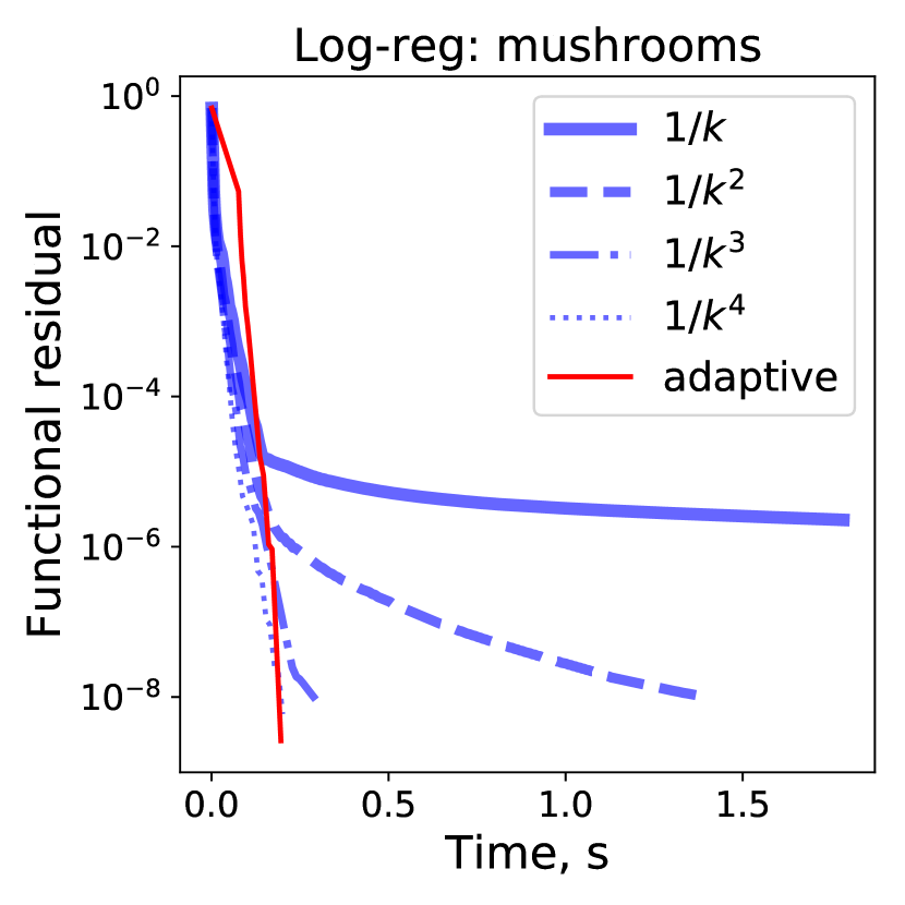
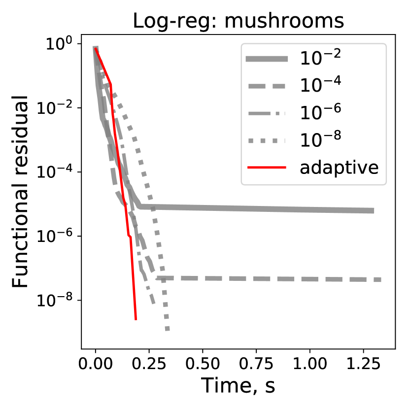
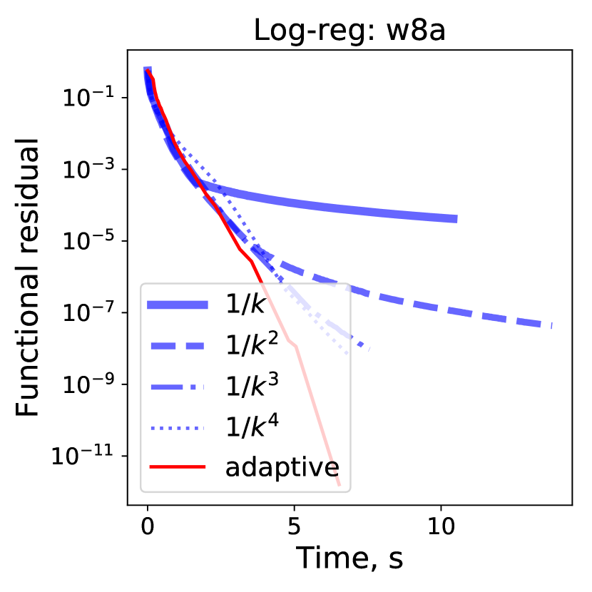
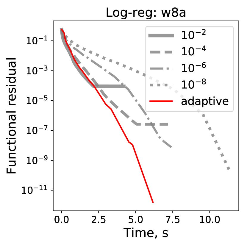
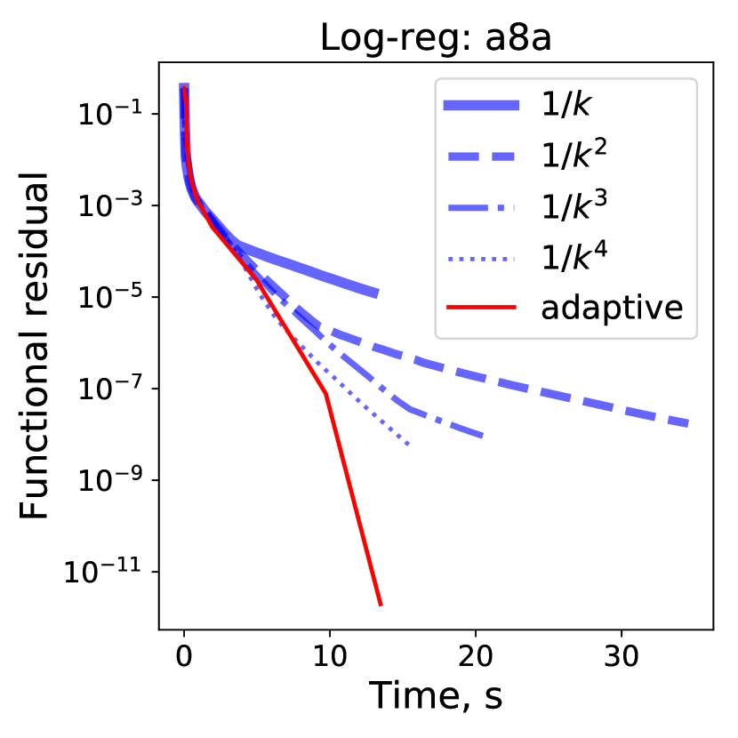
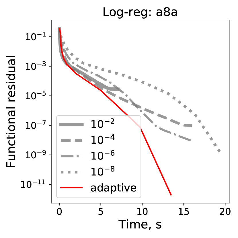
Figure 1: Comparison of different accuracy policies for inexact Cubic Newton, training logistic regression.

5.2 Log-Sum-Exp

In the next set of experiments, we consider unconstrained minimization of the following objective:

$$\begin{array}[]{rcl}f_{\mu}(x)&=&\mu\ln\left(\sum\limits_{i=1}^{m}\exp\Bigl{(}\frac{\langle a_{i},x\rangle-b_{i}}{\mu}\Bigr{)}\right),\;\;x\in\mathbb{R}^{n},\end{array}$$

where $\mu>0$ is a smoothing parameter. To generate the data, we sample coefficients $\{\tilde{a}_{i}\}_{i=1}^{m}$ and $b$ randomly from the uniform distribution on $[-1,1]$. Then, we shift the parameters in a way to have the solution $x^{*}$ in the origin. Namely, using $\{\tilde{a}_{i}\}_{i=1}^{m}$ we form a preliminary function $\tilde{f}_{\mu}(x)$, and set $a_{i}:=\tilde{a}_{i}-\nabla\tilde{f}_{\mu}(0)$. Thus we essentially obtain $\nabla f_{\mu}(0)=0$.

We set $m=6n$, and $n=100$. In the method, we use the following Euclidean norm for the primal space: $\|x\|=\langle Bx,x\rangle^{1/2}$, with the matrix $B=\sum_{i=1}^{m}a_{i}a_{i}^{T}$, and fix regularization parameter $H$ being equal $1$. The results are shown on Figure 2.

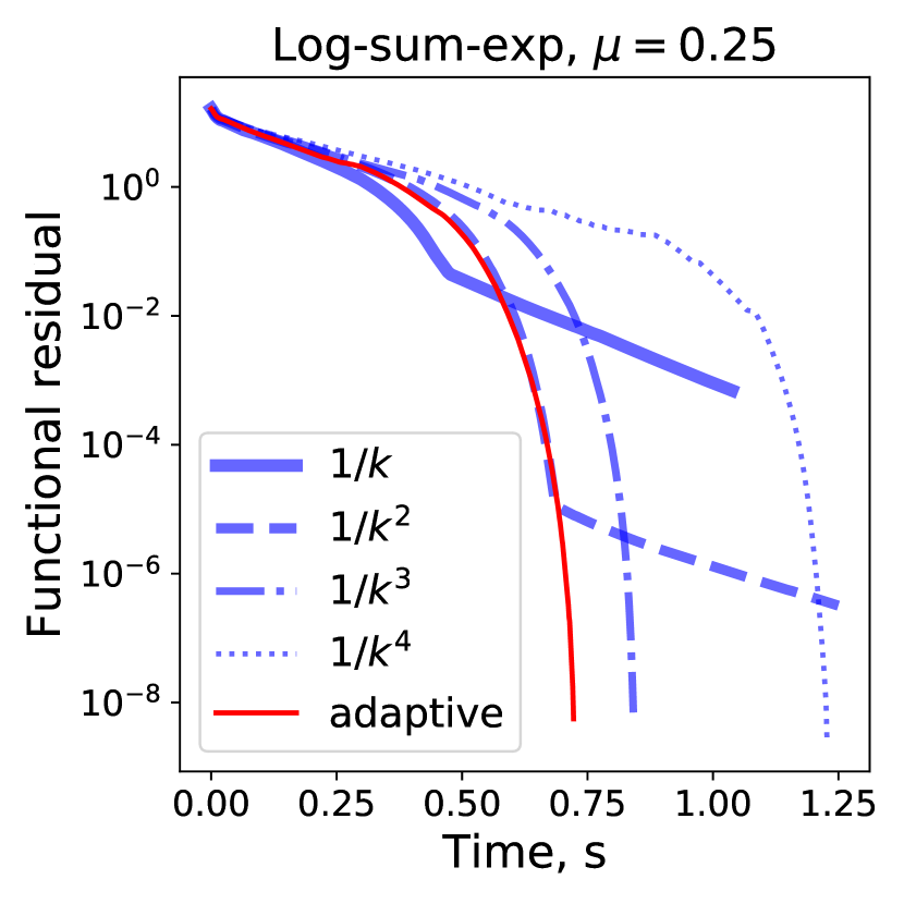
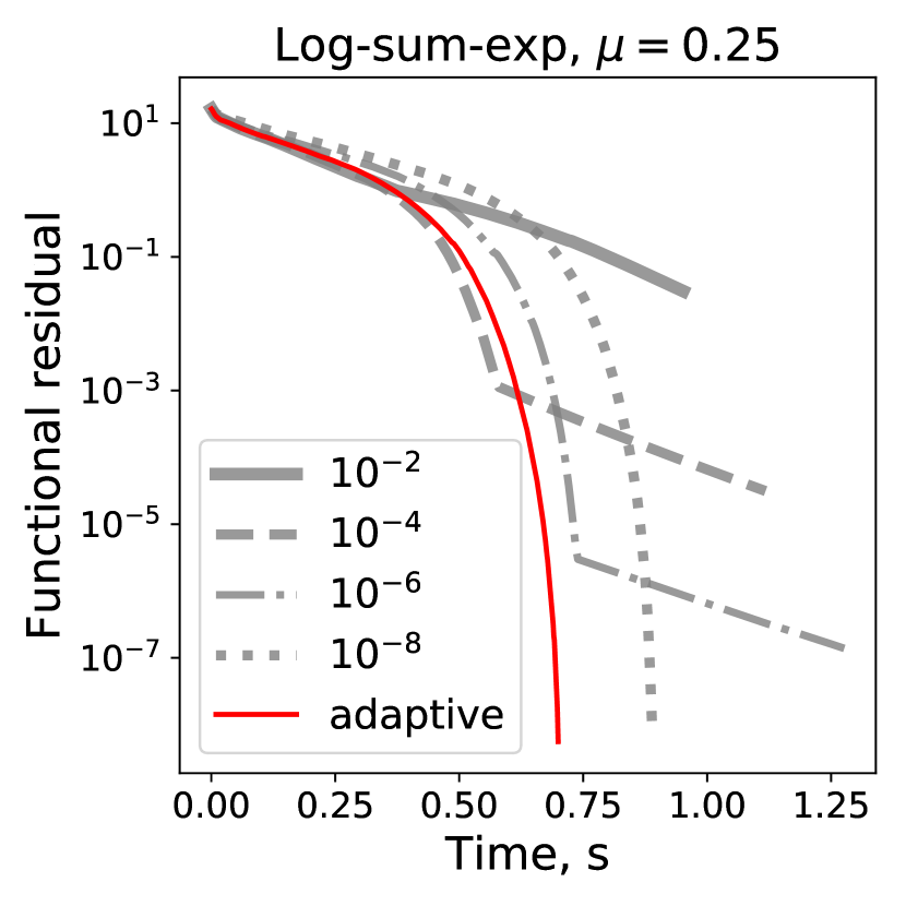
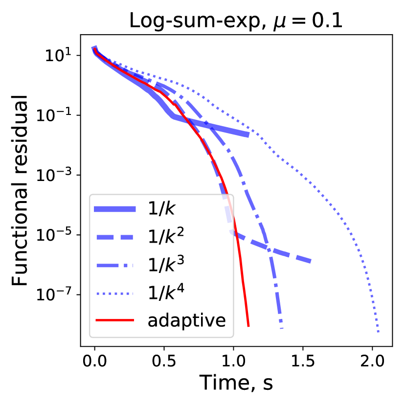
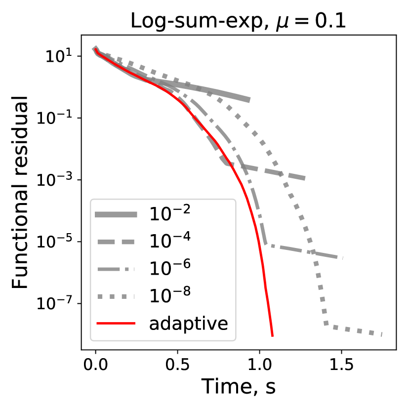
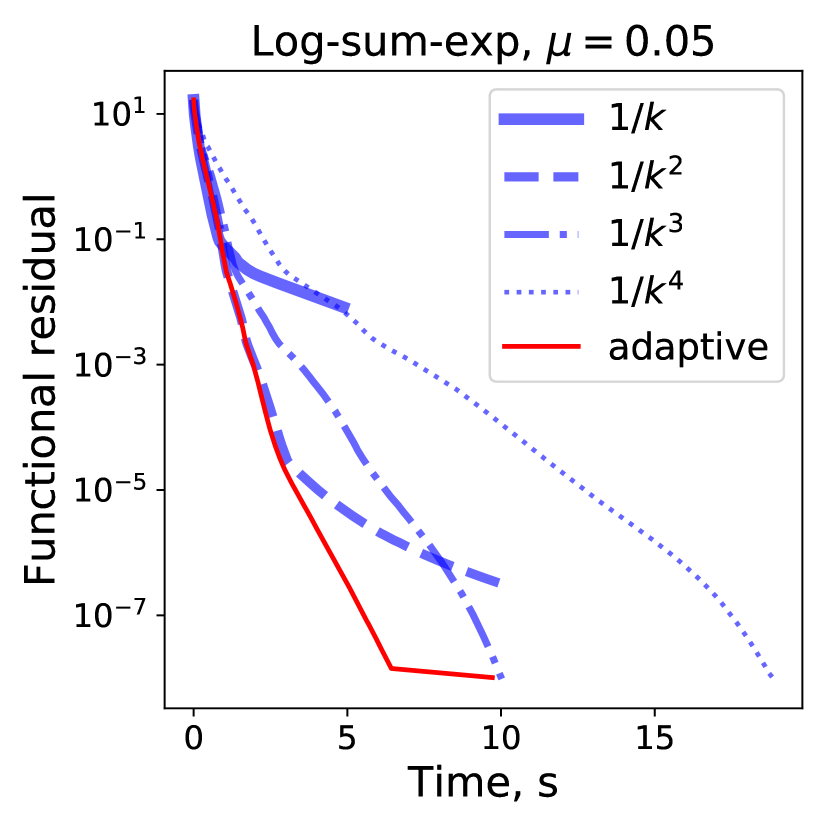
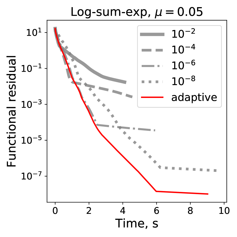
Figure 2: Comparison of different accuracy policies for inexact Cubic Newton, minimizing Log-Sum-Exp function.

We see, that the adaptive rule demonstrates reasonably good performance (in terms of the total computational time) in all the scenarios.

Appendix A Extra Experiments

A.1 Exact Stopping Criterion

In the following set of experiments with Cubic Newton method, we compute the exact minimizer of the model (5), at every iteration. Then, we use this value to ensure the required precision in function value of the subproblem for the inexact step (in the previous settings we used the upper bound (29) for this purpose). The results for Log-Sum-Exp function are shown on Figures 3 and 4. The results for Logistic regression are shown on Figure 5.

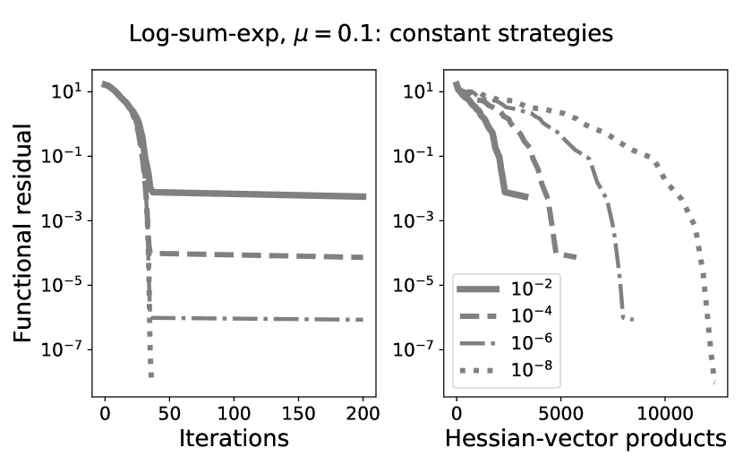
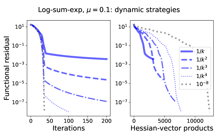
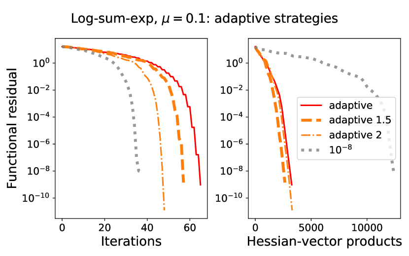
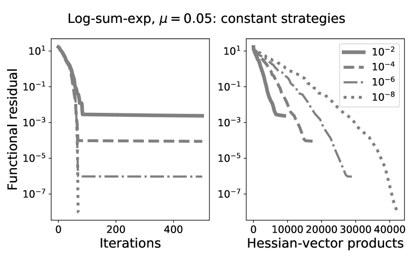
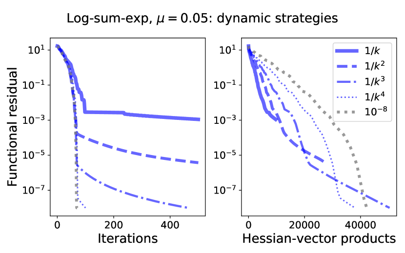
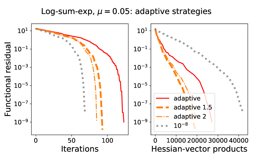
Figure 3: Exact stopping criterion, minimizing Log-Sum-Exp function, $n=100$.

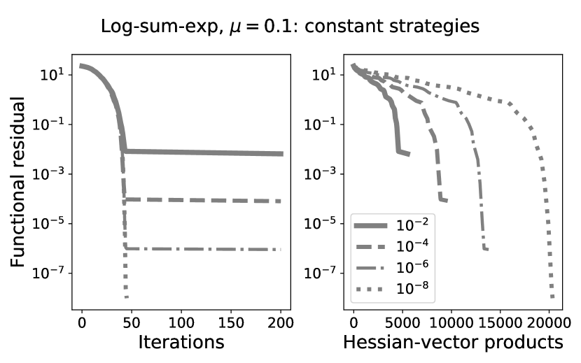
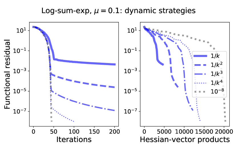
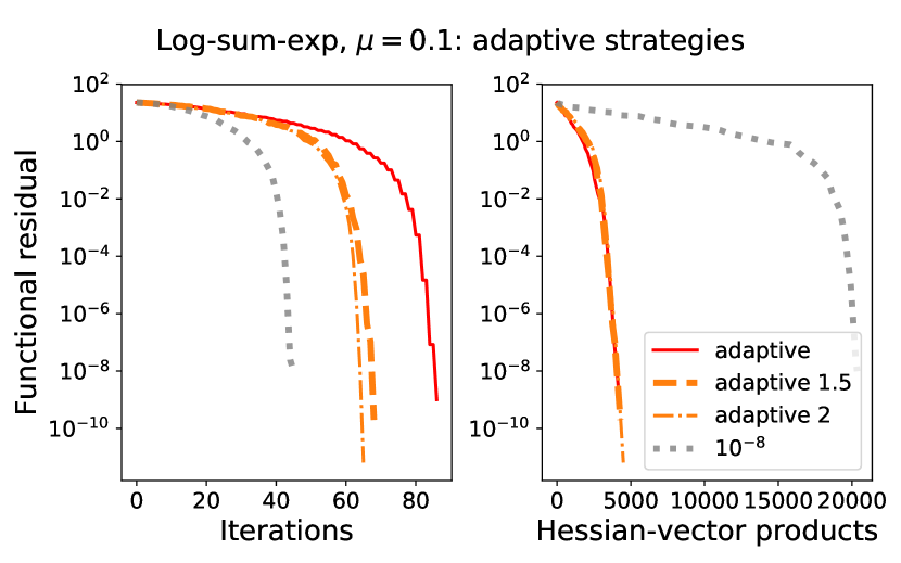
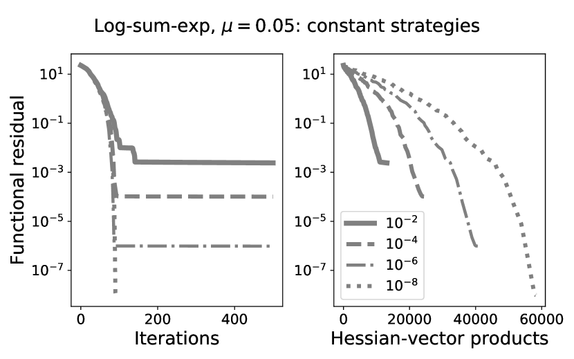
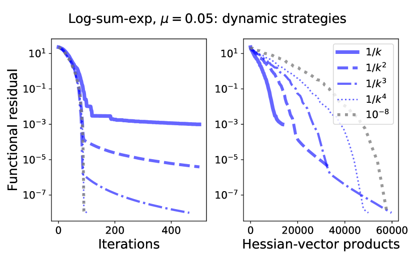
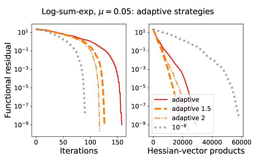
Figure 4: Exact stopping criterion, minimizing Log-Sum-Exp function, $n=200$.

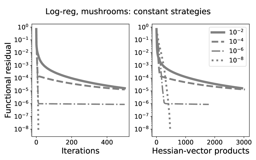
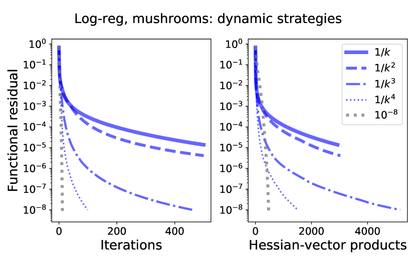
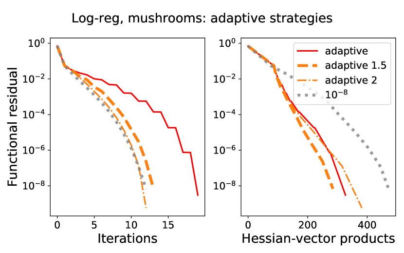
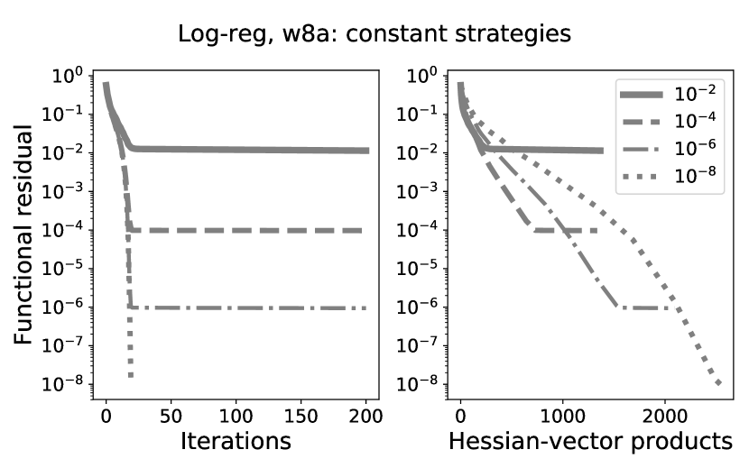
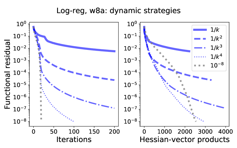
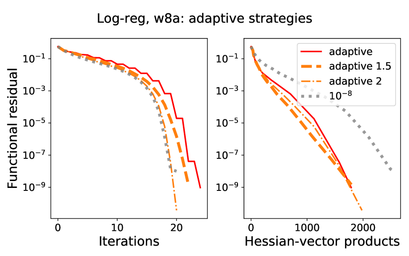
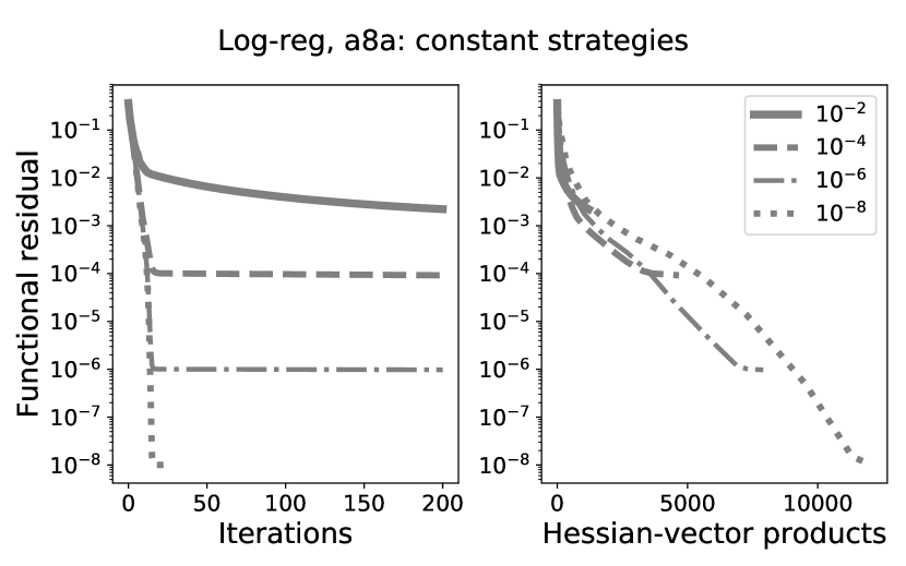
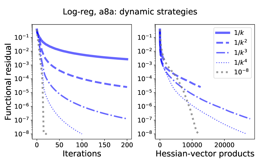
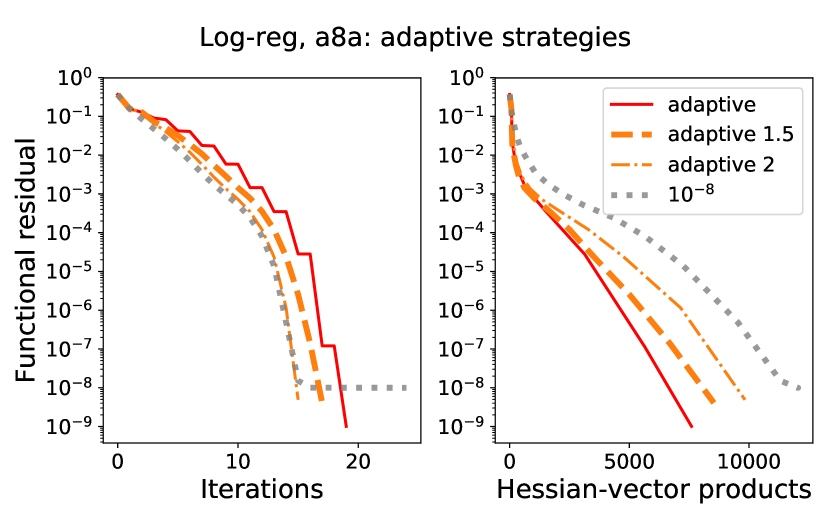
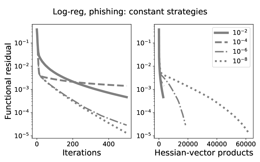
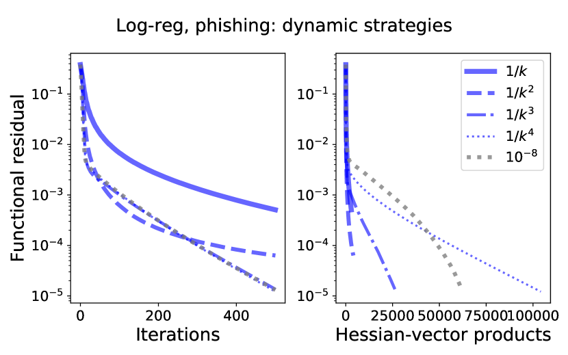
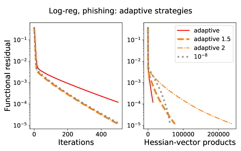
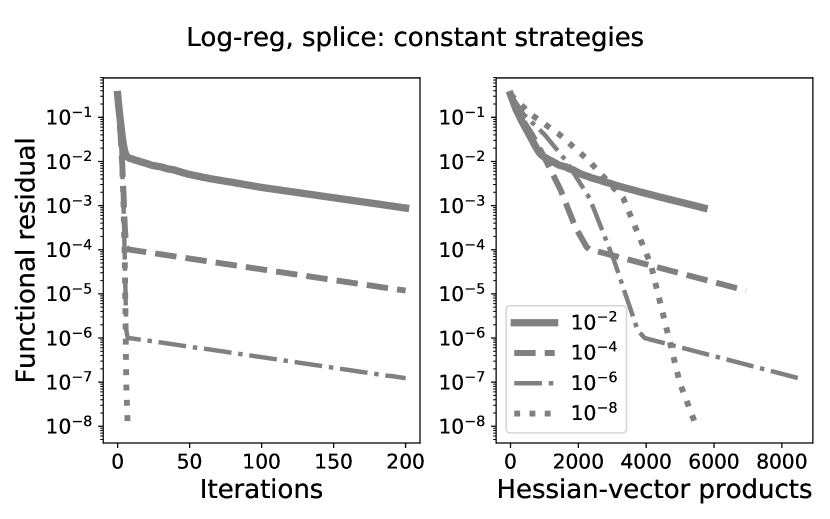
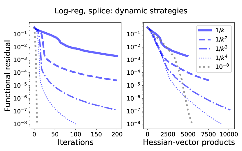
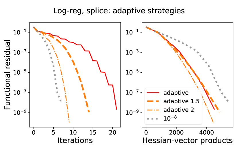
Figure 5: Exact stopping criterion, training Logistic regression.

We compare the iteration rate and the corresponding number of Hessian-vector products used, for the constant choice of inner accuracy (left graphs), dynamic strategies in the form $\delta_{k}=1/k^{\alpha}$ (center), and adaptive strategies $\delta_{k}=(F(x_{k-1})-F(x_{k}))^{\alpha}$ (right graphs). We use the names ”adaptive”, ”adaptive 1.5” and ”adaptive 2” for $\alpha=1$, $\alpha=3/2$, and $\alpha=2$, respectively.

We see, that the constant choice of inner accuracy reasonably depends on the desired precision for solving the initial problem. At the same time, the dynamic strategies are adjusting with the iterations. The best performance is achieved by the use of the adaptive policies. It is also notable, that in some cases, we need to use ”adaptive 1.5” or ”adaptive 2” strategy, to have the local superlinear convergence. This confirms our theory.

A.2 Averaging and Acceleration

In this experiment, we consider unconstrained minimization of the following objective ($x^{(i)}$ indicates $i$th coordinate of $x$)

$$\begin{array}[]{rcl}f(x)&=&|x^{(1)}|^{3}+\sum\limits_{i=2}^{n}|x^{(i)}-x^{(i-1)}|^{3},\qquad x\in\mathbb{R}^{n},\end{array}$$ (30)

by different inexact Newton methods. Note, that the structure of (30) is similar to that one of the worst function for the second-order methods (see Chapter 4.3.1 in (Nesterov, 2018)). It is also similar to the function from Example 6.

We compare iteration rates of the following algorithms: Cubic Newton (CN) with dynamic rule $\delta_{k}=1/k^{3}$, Cubic Newton with adaptive rule (14), the method with Averaging (Algorithm 3) with $\delta_{k}=1/k^{3}$, and the accelerated method with Contracting proximal iterations (Algorithm 4). For the latter one we use $\zeta_{k}=1/k$ and $\delta_{k}=1/k$, as the rules for choosing the accuracy of inexact (outer) proximal steps, and inexact (inner) Newton steps, respectively.

For the first three algorithms, we also compare the constant choice for the regularization parameter: $H=1$ (on the top graphs), and a simple line search for choosing $H$ at every iteration (bottom). The results are shown on Figure 6.

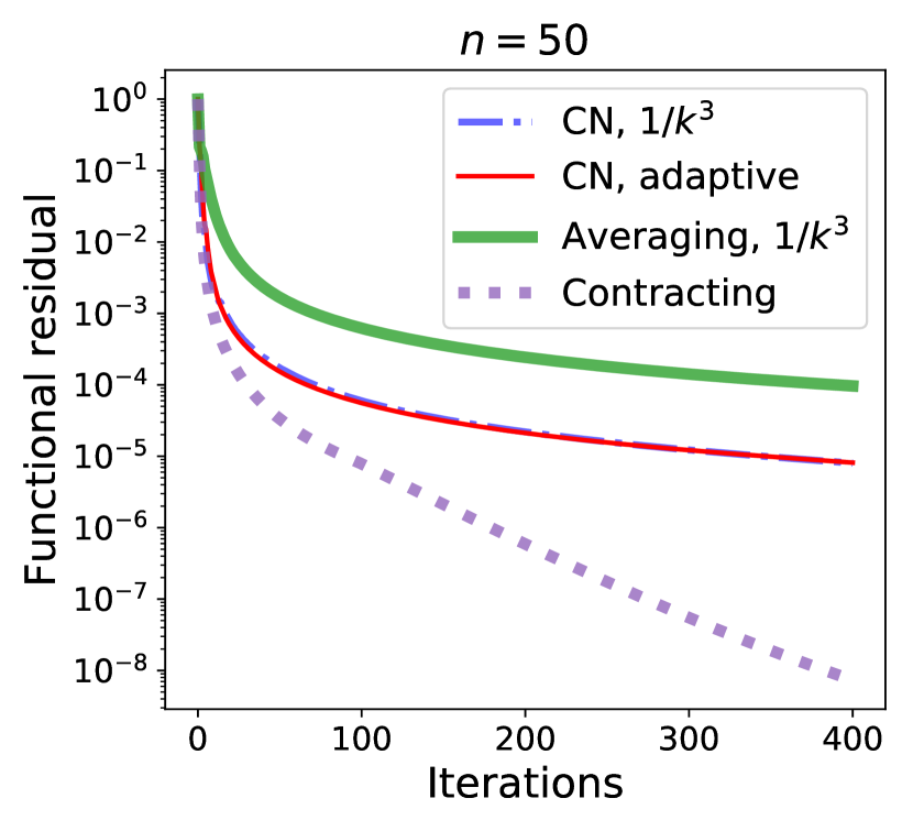
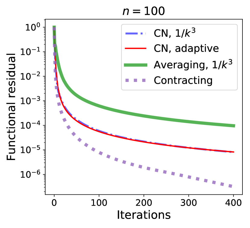
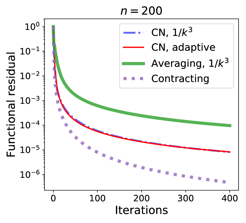
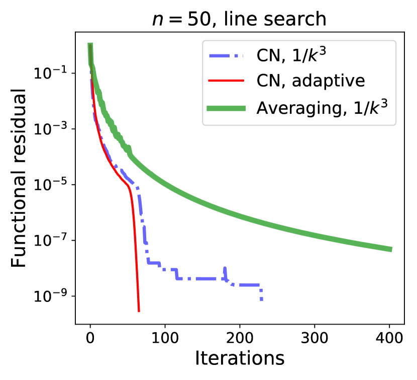
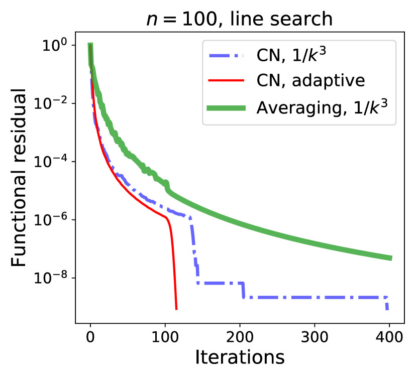
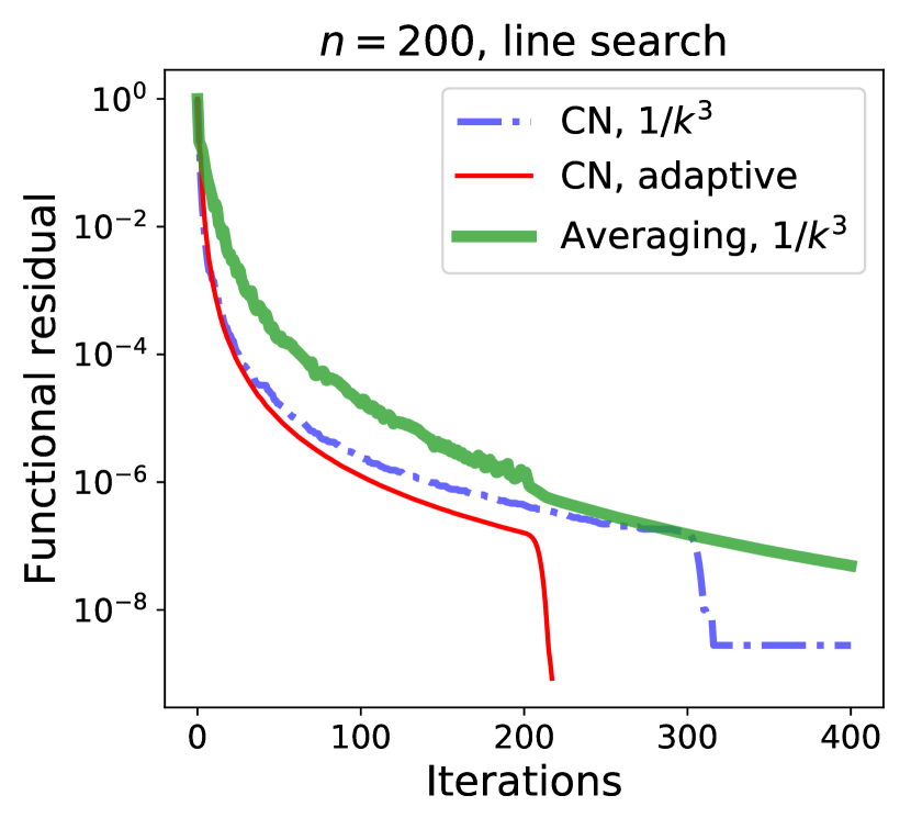
Figure 6: Methods with averaging and acceleration.

We see, that all the methods have a sublinear rate of convergence, until the iteration counter is smaller than the dimension of the problem. The use of the line search significantly helps for improving the rate. Thus, it seems to be an important open question (which we keep for the further research) — to equip the contracting proximal scheme (Algorithm 4) with a variant of line search as well.

Appendix B Auxiliary Results

Lemma 2

For every $a,b\geq 0$ and integer $p\geq 1$ it holds

$$\begin{array}[]{rcl}(a+b)^{p-1}&\leq&2^{p-2}a^{p-1}+2^{p-2}b^{p-1}.\end{array}$$ (31)

Proof:

For $p=1$ it is trivial. For $p\geq 2$ we use convexity of $y(x)=x^{p-1}$:

$$\begin{array}[]{rcl}\bigl{(}\frac{a+b}{2}\bigr{)}^{p-1}&\leq&\frac{a^{p-1}}{2}+\frac{b^{p-1}}{2},\end{array}$$

which is (31). $\Box$

Lemma 3

For every $s>1$, it holds

$$\begin{array}[]{rcl}\sum\limits_{i=1}^{k}\frac{1}{i^{s}}&\leq&\frac{s}{s-1}.\end{array}$$ (32)

Proof:

Indeed,

$$\begin{array}[]{rcl}\sum\limits_{i=1}^{k}\frac{1}{i^{s}}\;\;=\;\;1+\sum\limits_{i=2}^{k}\frac{1}{i^{s}}&\leq&1+\int\limits_{1}^{+\infty}\frac{dx}{x^{s}}\;\;=\;\;\frac{s}{s-1}.\end{array}$$

$\Box$

Lemma 4

For a given $a_{i}\in\mathbb{E}^{*}$, $1\leq i\leq m$, consider the log-sum-exp function

$$\begin{array}[]{rcl}f(x)&=&\log\left(\sum\limits_{i=1}^{m}e^{\langle a_{i},x\rangle}\right),\quad x\in\mathbb{E}.\end{array}$$

Then, for Euclidean norm $\|x\|=\langle Bx,x\rangle^{1/2},x\in\mathbb{E}$ with $B=\sum\limits_{i=1}^{m}a_{i}a_{i}^{*}$ (assuming $B\succ 0$, otherwise we can reduce dimensionality of the problem), we have the following estimates for the Lipschitz constants:

$$\begin{array}[]{rcccccl}L_{1}&=&1,\qquad L_{2}&=&2,\qquad L_{3}&=&4.\end{array}$$

Proof:

Denote $\kappa(x)=\sum_{i=1}^{m}e^{\langle a_{i},x\rangle}$. Then, for all $x\in\mathbb{E}$ and $h\in\mathbb{E}$, we have

$$\begin{array}[]{rcl}\langle\nabla f(x),h\rangle&=&\frac{1}{\kappa(x)}\sum\limits_{i=1}^{m}e^{\langle a_{i},x\rangle}\langle a_{i},h\rangle,\\ \\ \langle\nabla^{2}f(x)h,h\rangle&=&\frac{1}{\kappa(x)}\sum\limits_{i=1}^{m}e^{\langle a_{i},x\rangle}(\langle a_{i},h\rangle-\langle\nabla f(x),h\rangle)^{2}\;\;\leq\;\;\sum\limits_{i=1}^{m}\langle a_{i},h\rangle^{2}\;\;=\;\;\|h\|^{2},\\ \\ D^{3}f(x)[h]^{3}&=&\frac{1}{\kappa(x)}\sum\limits_{i=1}^{m}e^{\langle a_{i},x\rangle}(\langle a_{i},h\rangle-\langle\nabla f(x),h\rangle)^{3}\;\;\leq\;\;\langle\nabla^{2}f(x)h,h\rangle\max\limits_{1\leq i,j\leq m}\langle a_{i}-a_{j},h\rangle\;\;\leq\;\;2\|h\|^{3},\\ \\ D^{4}f(x)[h]^{4}&=&\frac{1}{\kappa(x)}\sum\limits_{i=1}^{m}e^{\langle a_{i},x\rangle}(\langle a_{i},h\rangle-\langle\nabla f(x),h\rangle)^{4}-3\langle\nabla^{2}f(x)h,h\rangle^{2}\\ \\ &\leq&D^{3}f(x)[h]^{3}\max\limits_{1\leq i,j\leq m}\langle a_{i}-a_{j},h\rangle\;\;\leq\;\;4\|h\|^{4}.\end{array}$$

$\Box$

Lemma 5

Let $\psi(x)=\frac{\mu}{2}\|x-x_{0}\|^{2}$, $\mu\geq 0$. Consider the ball of radius $D$ around some fixed point $c$:

$$\begin{array}[]{rcl}\mathcal{B}&=&\{x:\|x-c\|\leq D\}.\end{array}$$

Then, for any $p\geq 1$, it holds,

$$\begin{array}[]{rcl}\psi(y)-\psi(x)-\langle\nabla\psi(x),y-x\rangle&\geq&\frac{\sigma_{p+1}}{p+1}\|y-x\|^{p+1},\qquad x,y\in\mathcal{B},\end{array}$$

with $\sigma_{p+1}=\frac{(p+1)\mu}{2^{p}D^{p-1}}$. Thus function $\psi$ is uniformly convex of degree $p+1$ on a ball.

Proof:

For all $x,y\in\mathcal{B}$, we have

$$\begin{array}[]{rcl}\|x-y\|&\leq&\|x-c\|+\|c-y\|\;\;\leq\;\;2D.\end{array}$$

Therefore,

$$\begin{array}[]{rcl}\psi(y)-\psi(x)-\langle\nabla\psi(x),y-x\rangle&=&\frac{\mu}{2}\|y-x\|^{2}\\ \\ &=&\frac{\mu}{2\|y-x\|^{p-1}}\|y-x\|^{p+1}\\ \\ &\geq&\frac{\mu}{2^{p}D^{p-1}}\|y-x\|^{p+1}\;\;=\;\;\frac{\sigma_{p+1}}{p+1}\|y-x\|^{p+1}.\end{array}$$

$\Box$

Appendix C Proof of Theorem 1

Proof:

Indeed, by Lemma 1, for every $y\in{\rm dom\,}\psi$ we have

$$\begin{array}[]{rcl}F(x_{k+1})&\leq&F(T_{k+1})\;\;\stackrel{{\scriptstyle(\ref{OneStep})}}{{\leq}}\;\;F(y)+\frac{L_{p}\|y-x_{k}\|^{p+1}}{p!}+\delta_{k+1},\quad k\geq 0.\end{array}$$ (33)

Let us introduce an arbitrary sequence of positive increasing coefficients $\{A_{k}\}_{k\geq 0}$, $A_{0}\stackrel{{\scriptstyle\mathrm{def}}}{{=}}0$. Denote $a_{k+1}\stackrel{{\scriptstyle\mathrm{def}}}{{=}}A_{k+1}-A_{k}$. Then, plugging $y=\frac{a_{k+1}x^{*}+A_{k}x_{k}}{A_{k+1}}$ into (33), we obtain

$$\begin{array}[]{rcl}F(x_{k+1})&\leq&\frac{a_{k+1}}{A_{k+1}}F^{*}+\frac{A_{k}}{A_{k+1}}F(x_{k})+\frac{a_{k+1}^{p+1}}{A_{k+1}^{p+1}}\frac{L_{p}\|x_{k}-x^{*}\|^{p+1}}{p!}+\delta_{k+1},\end{array}$$

or, equivalently

$$\begin{array}[]{rcl}A_{k+1}(F(x_{k+1})-F^{*})&\leq&A_{k}(F(x_{k})-F^{*})+\frac{a_{k+1}^{p+1}}{A_{k+1}^{p}}\frac{L_{p}\|x_{k}-x^{*}\|^{p+1}}{p!}+A_{k+1}\delta_{k+1}.\end{array}$$

Summing up these inequalities, we get, for every $k\geq 1$

$$\begin{array}[]{rcl}A_{k}(F(x_{k})-F^{*})&\leq&\sum\limits_{i=1}^{k}A_{i}\delta_{i}+\frac{L_{p}}{p!}\sum\limits_{i=1}^{k}\frac{a_{i}^{p+1}}{A_{i}^{p}}\|x_{i}-x^{*}\|^{p+1}\\ \\ &\leq&\sum\limits_{i=1}^{k}A_{i}\delta_{i}+\frac{L_{p}D^{p+1}}{p!}\sum\limits_{i=1}^{k}\frac{a_{i}^{p+1}}{A_{i}^{p}},\end{array}$$ (34)

where the last inequality holds due to monotonicity of the method:

$$\begin{array}[]{rcl}F(x_{i})&\leq&F(x_{0}),\qquad i\geq 0.\end{array}$$

Finally, let us fix $A_{k}\equiv k^{p+1}$. Then, by the mean value theorem, for some $\xi\in[k-1;k]$

$$\begin{array}[]{rcl}a_{k}&=&A_{k}-A_{k-1}\;\;=\;\;k^{p+1}-(k-1)^{p+1}\\ \\ &=&(p+1)\xi^{p}\;\;\leq\;\;(p+1)k^{p}.\end{array}$$

Therefore,

$$\begin{array}[]{rcl}\sum\limits_{i=1}^{k}\frac{a_{i}^{p+1}}{A_{i}^{p}}&\leq&\sum\limits_{i=1}^{k}\frac{(p+1)^{p+1}i^{p(p+1)}}{i^{(p+1)p}}\;\;=\;\;(p+1)^{p+1}k,\end{array}$$ (35)

and

$$\begin{array}[]{rcl}\sum\limits_{i=1}^{k}A_{i}\delta_{i}&=&\sum\limits_{i=1}^{k}\frac{ci^{p+1}}{i^{p+1}}\;\;=\;\;ck.\end{array}$$ (36)

Plugging these bounds into (34) completes the proof. $\Box$

Appendix D Proof of Theorem 2

Proof:

First, by the same reasoning as in Theorem 1, we obtain the following bound, for every $k\geq 1$:

$$\begin{array}[]{rcl}A_{k}(F(x_{k})-F^{*})&\leq&\sum\limits_{i=1}^{k}A_{i}\delta_{i}+\frac{L_{p}D^{p+1}}{p!}\sum\limits_{i=1}^{k}\frac{a_{i}^{p+1}}{A_{i}^{p}},\end{array}$$ (37)

where $\{A_{k}\}_{k\geq 0}$ is an arbitrary sequence of increasing coefficients, with $A_{0}\stackrel{{\scriptstyle\mathrm{def}}}{{=}}0$, and $a_{k}\stackrel{{\scriptstyle\mathrm{def}}}{{=}}A_{k}-A_{k-1}$.

Substituting into (37) the values $\delta_{i}=c(F(x_{i-2})-F(x_{i-1})),\;i\geq 2$, we have

$$\begin{array}[]{rcl}A_{k}(F(x_{k})-F^{*})&\leq&A_{1}\delta_{1}+c\sum\limits_{i=2}^{k}A_{i}(F(x_{i-2})-F(x_{i-1}))+\frac{L_{p}D^{p+1}}{p!}\sum\limits_{i=1}^{k}\frac{a_{i}^{p+1}}{A_{i}^{p}},\quad k\geq 1,\end{array}$$ (38)

or, rearranging the terms, it holds for every $k\geq 2$:

$$\begin{array}[]{cl}&(c+1)A_{k}(F(x_{k})-F^{*})\\ \\ &\quad\;\;\,\,\leq\;\;\,\,A_{k}(F(x_{k})-F^{*})+cA_{k}(F(x_{k-1})-F^{*})\\ \\ &\quad\;\;\stackrel{{\scriptstyle(\ref{eq-th2-main})}}{{\leq}}\;\;\frac{L_{p}D^{p+1}}{p!}\sum\limits_{i=1}^{k}\frac{a_{i}^{p+1}}{A_{i}^{p}}+c\sum\limits_{i=1}^{k-2}(A_{i+2}-A_{i+1})(F(x_{i})-F^{*})+A_{1}\delta_{1}+cA_{2}(F(x_{0})-F^{*})\\ \\ &\quad\;\;\,\,=\;\;\,\,\frac{L_{p}D^{p+1}}{p!}\sum\limits_{i=1}^{k}\frac{a_{i}^{p+1}}{A_{i}^{p}}+c\sum\limits_{i=1}^{k-2}a_{i+2}(F(x_{i})-F^{*})+A_{1}\delta_{1}+cA_{2}(F(x_{0})-F^{*}),\end{array}$$ (39)

and for $k=1$ we have

$$\begin{array}[]{rcl}A_{1}(F(x_{1})-F^{*})&\stackrel{{\scriptstyle(\ref{eq-th2-main})}}{{\leq}}&A_{1}\delta_{1}+\frac{L_{p}D^{p+1}}{p!}\frac{a_{1}^{p+1}}{A_{1}^{p}}\;\;=\;\;A_{1}\Bigl{(}\delta_{1}+\frac{L_{p}D^{p+1}}{p!}\Bigr{)}.\end{array}$$ (40)

Now, let us pick $A_{k}\equiv k^{p+2}$. Then,

$$\begin{array}[]{rcl}a_{k}&\equiv&k^{p+2}-(k-1)^{p+2}\;\;\leq\;\;(p+2)k^{p+1},\end{array}$$

and

$$\begin{array}[]{rcl}\sum\limits_{i=1}^{k}\frac{a_{i}^{p+1}}{A_{i}^{p}}&\leq&(p+2)^{p+1}\sum\limits_{i=1}^{k}\frac{i^{(p+1)^{2}}}{i^{(p+2)p}}\;\;=\;\;(p+2)^{p+1}\sum\limits_{i=1}^{k}i\;\;\leq\;\;(p+2)^{p+1}k^{2}.\end{array}$$

Therefore, (39) leads to

$$\begin{array}[]{cl}&(c+1)k^{p+2}(F(x_{k})-F^{*})\\ \\ &\quad\;\;\,\,\leq\;\;\,\,\frac{(p+2)^{p+1}k^{2}L_{p}D^{p+1}}{p!}+c(p+2)\sum\limits_{i=1}^{k-2}(i+2)^{p+1}(F(x_{i})-F^{*})+\delta_{1}+c2^{p+2}(F(x_{0})-F^{*}),\quad k\geq 2.\end{array}$$ (41)

And the statement to be proved is

$$\begin{array}[]{rcl}F(x_{k})-F^{*}&\leq&\frac{\beta}{k^{p+2}}+\frac{\gamma L_{p}D^{p+1}}{p!\,k^{p}},\quad k\geq 1,\end{array}$$ (42)

where

$$\begin{array}[]{rcl}\beta&\stackrel{{\scriptstyle\mathrm{def}}}{{=}}&\frac{\delta_{1}+c2^{p+2}(F(x_{0})-F^{*})}{1-c((p+2)^{2}/(p+1)-1)},\qquad\gamma\;\;\stackrel{{\scriptstyle\mathrm{def}}}{{=}}\;\;\frac{(p+2)^{p+1}}{1-c((p+2)3^{p+1}-1)}.\end{array}$$ (43)

Note, that from our assumptions, $c$ is small enough: $c\leq\frac{1}{(p+2)3^{p+1}-1}$, and (43) are correctly defined.

Let us prove (42) by induction. It holds for $k=1$ by (40). Assuming that it holds for all $1\leq k\leq K-2$, we have

$$\begin{array}[]{rcl}F(x_{K})-F^{*}&\overset{\eqref{eq-th2-main-3},\eqref{eq-th2-prove}}{\leq}&\frac{(p+2)^{p+1}L_{p}D^{p+1}}{(c+1)\,p!\,K^{p}}+\frac{c(p+2)}{(c+1)K^{p+2}}\sum\limits_{i=1}^{K-2}(i+2)^{p+1}\Bigl{(}\frac{\gamma L_{p}D^{p+1}}{p!\,i^{p}}+\frac{\beta}{i^{p+2}}\Bigr{)}+\frac{\delta_{1}+c2^{p+2}(F(x_{0})-F^{*})}{(c+1)K^{p+2}}\\ \\ &=&\Bigl{(}\frac{(p+2)^{p+1}}{c+1}+\frac{\gamma c(p+2)}{(c+1)K^{2}}\sum\limits_{i=1}^{K-2}\frac{(i+2)^{p+1}}{i^{p}}\Bigr{)}\cdot\frac{L_{p}D^{p+1}}{p!\,K^{p}}\\ \\ &&\quad+\quad\Bigl{(}\frac{\beta c(p+2)}{(c+1)}\sum\limits_{i=1}^{K-2}\frac{1}{i^{p+2}}+\frac{\delta_{1}+c2^{p+2}(F(x_{0})-F^{*})}{c+1}\Bigr{)}\cdot\frac{1}{K^{p+2}}\\ \\ &\leq&\frac{(p+2)^{p+1}+\gamma c(p+2)3^{p+1}}{c+1}\cdot\frac{L_{p}D^{p+1}}{p!\,K^{p}}+\Bigl{(}\frac{\beta c(p+2)^{2}}{(c+1)(p+1)}+\frac{\delta_{1}+c2^{p+2}(F(x_{0})-F^{*})}{c+1}\Bigr{)}\frac{1}{K^{p+2}},\end{array}$$

where we have used in the last inequality the following simple bounds:

$$\begin{array}[]{rcl}\sum\limits_{i=1}^{K-2}\frac{(i+2)^{p+1}}{i^{p}}&\leq&3^{p+1}\sum\limits_{i=1}^{K-2}\frac{i^{p+1}}{i^{p}}\;\;\leq\;\;3^{p+1}K^{2},\\ \\ \sum\limits_{i=1}^{K-2}\frac{1}{i^{p+2}}&\stackrel{{\scriptstyle(\ref{SublinBound})}}{{\leq}}&\frac{p+2}{p+1}.\end{array}$$

Therefore, to finish the proof, its enough to verify two equations:

$$\begin{array}[]{rcl}\frac{\beta c(p+2)^{2}}{(c+1)(p+1)}+\frac{\delta_{1}+c2^{p+2}(F(x_{0})-F^{*})}{c+1}&=&\beta,\quad\text{and}\quad\frac{(p+2)^{p+1}+\gamma c(p+2)3^{p+1}}{c+1}\;\;=\;\;\gamma.\end{array}$$

which are (43). $\Box$

Appendix E Proof of Theorem 3

Proof:

Indeed, by Lemma 1, for every $y\in{\rm dom\,}\psi$ we have

$$\begin{array}[]{rcl}F(x_{k+1})&\leq&F(y)+\frac{L_{p}\|y-x_{k}\|^{p+1}}{p!}+\delta_{k+1},\quad k\geq 0.\end{array}$$ (44)

Let us substitute $y=\lambda x^{*}+(1-\lambda)x_{k}$ into (44), where $\lambda\equiv\omega_{p}^{-1/p}\in(0,1]$. This gives

$$\begin{array}[]{rcl}F(x_{k+1})&\leq&\lambda F^{*}+(1-\lambda)F(x_{k})+\frac{\lambda^{p+1}L_{p}\|x_{k}-x^{*}\|^{p+1}}{p!}+\delta_{k+1}\\ \\ &\leq&\lambda F^{*}+(1-\lambda)F(x_{k})+\frac{\lambda^{p+1}(p+1)L_{p}}{\sigma_{p+1}p!}(F(x_{k})-F^{*})+\delta_{k+1},\end{array}$$

where we use uniform convexity in the last inequality. Therefore, for every $k\geq 1$:

$$\begin{array}[]{rcl}F(x_{k+1})-F^{*}&\leq&\Bigl{(}1-\omega_{p}^{-1/p}+\frac{\omega_{p}^{-1/p}}{p+1}\Bigr{)}(F(x_{k})-F^{*})+\delta_{k+1}\\ \\ &=&\Bigl{(}1-\frac{p}{p+1}\omega_{p}^{-1/p})(F(x_{k})-F^{*})+c(F(x_{k-1})-F(x_{k}))\\ \\ &\leq&\Bigl{(}1-\frac{p}{p+1}\omega_{p}^{-1/p}+c\Bigr{)}(F(x_{k-1})-F^{*}),\end{array}$$

the last inequality uses monotonicity of the method: $F(x_{k})\leq F(x_{k-1})$ and the bound: $F^{*}\leq F(x_{k})$. $\Box$

Appendix F Proof of Theorem 4

Proof:

Let us plug $y=x^{*}$ into (7). Thus, we obtain, for every $k\geq 1$:

$$\begin{array}[]{rcl}F(x_{k+1})&\leq&F^{*}+\frac{L_{p}\|x_{k}-x^{*}\|^{p+1}}{p!}+\delta_{k+1}\\ \\ &\leq&F^{*}+\frac{L_{p}}{p!}\bigl{(}\frac{2}{\sigma_{2}}\bigr{)}^{p+1\over 2}(F(x_{k})-F^{*})^{p+1\over 2}+\delta_{k+1}\\ \\ &=&F^{*}+\frac{L_{p}}{p!}\bigl{(}\frac{2}{\sigma_{2}}\bigr{)}^{p+1\over 2}(F(x_{k})-F^{*})^{p+1\over 2}+c(F(x_{k-1})-F(x_{k}))^{p+1\over 2}\\ \\ &\leq&F^{*}+\Bigl{(}\frac{L_{p}}{p!}\bigl{(}\frac{2}{\mu}\bigr{)}^{p+1\over 2}+c\Bigr{)}(F(x_{k-1})-F^{*})^{p+1\over 2},\end{array}$$

where monotonicity of the method: $F(x_{k})\leq F(x_{k-1})$ and the bound: $F^{*}\leq F(x_{k})$ are used in the last inequality. $\Box$

Appendix G Proof of Theorem 5

Proof:

The proof is similar to that one of Theorem 1.

By Lemma 1, for every $y\in{\rm dom\,}\psi$ we have

$$\begin{array}[]{rcl}F(x_{k+1})&\stackrel{{\scriptstyle(\ref{OneStep})}}{{\leq}}&F(y)+\frac{L_{p}\|y-y_{k}\|^{p+1}}{p!}+\delta_{k+1},\quad k\geq 0.\end{array}$$

Let us substitute $y=\lambda_{k}x_{k}+(1-\lambda_{k})x^{*}$, with $\lambda_{k}$ defined in the algorithm:

$$\begin{array}[]{rcl}\lambda_{k}&\equiv&\bigl{(}\frac{k}{k+1}\bigr{)}^{p+1}.\end{array}$$

Thus we obtain

$$\begin{array}[]{rcl}F(x_{k+1})&\leq&(1-\lambda_{k})F^{*}+\lambda_{k}F(x_{k})+(1-\lambda_{k})^{p+1}\frac{L_{p}\|x_{0}-x^{*}\|^{p+1}}{p!}+\delta_{k+1},\end{array}$$

or, equivalently

$$\begin{array}[]{rcl}A_{k+1}(F(x_{k+1})-F^{*})&\leq&A_{k}(F(x_{k})-F^{*})+\frac{a_{k+1}^{p+1}}{A_{k+1}^{p}}\frac{L_{p}\|x_{0}-x^{*}\|^{p+1}}{p!}+A_{k+1}\delta_{k+1},\end{array}$$

where $A_{k}\equiv k^{p+1}$ and $a_{k}\equiv A_{k}-A_{k-1}$ (so it holds: $\lambda_{k}\equiv{A_{k}}/{A_{k+1}}$ and $1-\lambda_{k}\equiv{a_{k+1}}/{A_{k+1}}$). Telescoping these inequalities and using the bounds (35) and (36) complete the proof. $\Box$

Appendix H Proof of Theorem 6

Proof:

The proof is similar to that one of Theorem 1 from (Doikov & Nesterov, 2019a), where convergence rate of Contracting Proximal Method is established. Additional technical difficulties, which are arising here, are caused by using inexact solution of the subproblem, equipped with the stopping condition (25).

We denote the optimal point of $h_{k+1}(\cdot)$ by $z_{k+1}\stackrel{{\scriptstyle\mathrm{def}}}{{=}}\mathop{\rm argmin}_{y\in\mathbb{E}}h_{k+1}(y)$. Since the next prox-center $v_{k+1}$ is defined as an approximate minimizer, we have

$$\begin{array}[]{rcl}h_{k+1}(v_{k+1})-h_{k+1}(z_{k+1})&\leq&\zeta_{k+1}.\end{array}$$ (45)

Function $h_{k+1}(\cdot)$ is strongly convex with respect to $d(\cdot)$, thus we have

$$\begin{array}[]{rcl}\zeta_{k+1}&\stackrel{{\scriptstyle(\ref{eq:th6hmin})}}{{\geq}}&h_{k+1}(v_{k+1})-h_{k+1}(z_{k+1})\;\;\geq\;\;\beta_{d}(z_{k+1};v_{k+1})\\ \\ &\geq&\frac{1}{2^{p-1}(p+1)}\|v_{k+1}-z_{k+1}\|^{p+1}.\end{array}$$ (46)

Therefore,

$$\begin{array}[]{rcl}\|v_{k+1}-z_{k+1}\|&\stackrel{{\scriptstyle(\ref{eq:th6PointsBound})}}{{\leq}}&\xi_{k+1}\;\;\stackrel{{\scriptstyle\mathrm{def}}}{{=}}\;\;2^{p-1\over p+1}(p+1)^{1\over p+1}\zeta_{k+1}^{1\over p+1}.\end{array}$$ (47)

Let us prove by induction the following inequality, for every $k\geq 0$:

$$\begin{array}[]{rcl}\beta_{d}(x_{0};x)+A_{k}F(x)&\geq&\beta_{d}(v_{k};x)+A_{k}F(x_{k})+C_{k}(x),\qquad x\in{\rm dom\,}F.\end{array}$$ (48)

where $C_{k}(x)\stackrel{{\scriptstyle\mathrm{def}}}{{=}}-\sum\limits_{i=1}^{k}\bigl{(}\tau_{i}\|x-v_{i}\|+\zeta_{i}\bigr{)}$, and $\tau_{i}\stackrel{{\scriptstyle\mathrm{def}}}{{=}}p2^{p-2}\|z_{i}-x_{0}\|^{p-1}\xi_{i}+2^{p-2}\xi_{i}^{p}$.

It obviously holds for $k=0$. Assume that it holds for the current iterate, and consider the next step $k+1$:

$$\begin{array}[]{rcl}&&\!\!\!\!\!\!\!\!\!\!\!\!\!\!\!\!\!\!\beta_{d}(x_{0};x)+A_{k+1}F(x)\\ \\ &=&\beta_{d}(x_{0};x)+A_{k}F(x)+a_{k+1}F(x)\\ \\ &\stackrel{{\scriptstyle(\ref{eq:th6inductive})}}{{\geq}}&\beta_{d}(v_{k};x)+A_{k}F(x_{k})+a_{k+1}F(x)+C_{k}(x)\\ \\ &\geq&\beta_{d}(v_{k};x)+A_{k+1}f\bigl{(}\frac{a_{k+1}x+A_{k}x_{k}}{A_{k+1}}\bigr{)}+a_{k+1}\psi(x)+A_{k}\psi(x_{k})+C_{k}(x)\\ \\ &=&h_{k+1}(x)+A_{k}\psi(x_{k})+C_{k}(x),\end{array}$$ (49)

where the last inequality holds by convexity of $f$.

Using strong convexity of $h_{k+1}(\cdot)$ with respect to $d(\cdot)$, we obtain

$$\begin{array}[]{rcl}h_{k+1}(x)&\geq&h_{k+1}(z_{k+1})+\beta_{d}(z_{k+1};x)\\ \\ &\stackrel{{\scriptstyle(\ref{eq:th6hmin})}}{{\geq}}&h_{k+1}(v_{k+1})+\beta_{d}(z_{k+1};x)-\zeta_{k+1}\\ \\ &=&h_{k+1}(v_{k+1})+\beta_{d}(v_{k+1};x)+\beta_{d}(z_{k+1};v_{k+1})+\langle\nabla d(v_{k+1})-\nabla d(z_{k+1}),x-v_{k+1}\rangle-\zeta_{k+1}\\ \\ &\geq&h_{k+1}(v_{k+1})+\beta_{d}(v_{k+1};x)-\|\nabla d(v_{k+1})-\nabla d(z_{k+1})\|_{*}\cdot\|x-v_{k+1}\|-\zeta_{k+1}.\end{array}$$ (50)

Now, computing second derivative of $d(x)=\frac{1}{p+1}\|x-x_{0}\|^{p+1}$, we get

$$\begin{array}[]{rcl}\nabla^{2}d(x)&=&(p-1)\|x-x_{0}\|^{p-3}B(x-x_{0})(x-x_{0})^{*}B+\|x-x_{0}\|^{p-1}B\\ \\ &\preceq&p\|x-x_{0}\|^{p-1}B.\end{array}$$ (51)

Therefore,

$$\begin{array}[]{rcl}\|\nabla d(v_{k+1})-\nabla d(z_{k+1})\|_{*}&=&\|\int\limits_{0}^{1}\nabla^{2}d(z_{k+1}+\tau(v_{k+1}-z_{k+1}))d\tau(v_{k+1}-z_{k+1})\|_{*}\\ \\ &\stackrel{{\scriptstyle(\ref{eq:th6xiDef})}}{{\leq}}&\xi_{k+1}\int\limits_{0}^{1}\|\nabla^{2}d(z_{k+1}+\tau(v_{k+1}-z_{k+1}))\|d\tau\\ \\ &\stackrel{{\scriptstyle(\ref{eq:th6dSecondDeriv})}}{{\leq}}&p\xi_{k+1}\int\limits_{0}^{1}\|z_{k+1}-x_{0}+\tau(v_{k+1}-z_{k+1})\|^{p-1}d\tau\\ \\ &\overset{\eqref{PoweredSumBound},\eqref{eq:th6xiDef}}{\leq}&p\xi_{k+1}\int\limits_{0}^{1}\bigl{(}2^{p-2}\|z_{k+1}-x_{0}\|^{p-1}+2^{p-2}\tau^{p-1}\xi_{k+1}^{p-1}\bigr{)}d\tau\\ \\ &=&p2^{p-2}\|z_{k+1}-x_{0}\|^{p-1}\xi_{k+1}+2^{p-2}\xi_{k+1}^{p}\;\;\stackrel{{\scriptstyle\mathrm{def}}}{{=}}\;\;\tau_{k+1}.\end{array}$$ (52)

Combining obtained bounds together, we conclude

$$\begin{array}[]{rcl}\beta_{d}(x_{0};x)+A_{k+1}F(x)&\stackrel{{\scriptstyle(\ref{eq:th6induction})}}{{\geq}}&h_{k+1}(x)+A_{k}\psi(x_{k})+C_{k}(x)\\ \\ &\overset{\eqref{eq:th6hStrongConv},\eqref{eq:th6LipGrad}}{\geq}&h_{k+1}(v_{k+1})+\beta_{d}(v_{k+1};x)-\tau_{k+1}\|x-v_{k+1}\|-\zeta_{k+1}+A_{k}\psi(x_{k})+C_{k}(x)\\ \\ &=&h_{k+1}(v_{k+1})+\beta_{d}(v_{k+1};x)+A_{k}\psi(x_{k})+C_{k+1}(x)\\ \\ &=&A_{k+1}f(x_{k+1})+a_{k+1}\psi(v_{k+1})+\beta_{d}(v_{k};v_{k+1})+\beta_{d}(v_{k+1};x)+A_{k}\psi(x_{k})+C_{k+1}(x)\\ \\ &\geq&A_{k+1}F(x_{k+1})+\beta_{d}(v_{k+1};x)+C_{k+1}(x).\end{array}$$

Thus, (48) is proven for all $k\geq 0$.

Let us plug $x:=x^{*}$ into (48). We obtain

$$\begin{array}[]{rcl}\beta_{d}(v_{k};x^{*})+A_{k}(F(x_{k})-F^{*})&\stackrel{{\scriptstyle(\ref{eq:th6inductive})}}{{\leq}}&\beta_{d}(x_{0};x^{*})-C_{k}(x^{*})\\ \\ &=&\beta_{d}(x_{0};x^{*})+\sum\limits_{i=1}^{k}\zeta_{i}+\sum\limits_{i=1}^{k}\tau_{i}\|v_{i}-x^{*}\|\\ \\ &\stackrel{{\scriptstyle(\ref{SublinBound})}}{{\leq}}&\beta_{d}(x_{0};x^{*})+\frac{c(p+2)}{p+1}+\sum\limits_{i=1}^{k}\tau_{i}\|v_{i}-x^{*}\|\;\;\stackrel{{\scriptstyle\mathrm{def}}}{{=}}\;\;\alpha_{k},\end{array}$$ (53)

and to finish the proof, we need to estimate $\alpha_{k}$ from above.

By uniform convexity of $d(\cdot)$, we have

$$\begin{array}[]{rcl}\frac{1}{2^{p-1}(p+1)}\|v_{k}-x^{*}\|^{p+1}&\leq&\beta_{d}(v_{k};x^{*})\;\;\stackrel{{\scriptstyle(\ref{eq:th6Main})}}{{\leq}}\;\;\alpha_{k}.\end{array}$$ (54)

At the same time,

$$\begin{array}[]{rcl}\alpha_{k}&=&\alpha_{k-1}+\tau_{k}\|v_{k}-x^{*}\|\;\;\stackrel{{\scriptstyle(\ref{eq:th6AlphaLower})}}{{\leq}}\;\;\alpha_{k-1}+2^{p-1\over p+1}(p+1)^{1\over p+1}\tau_{k}\alpha_{k}^{1\over p+1}.\end{array}$$

Dividing both sides of the last inequality by $\alpha_{k}^{1\over p+1}$, and using monotonicity of $\{\alpha_{k}\}_{k\geq 0}$, we get

$$\begin{array}[]{rcl}\alpha_{k}^{p\over p+1}&\leq&\alpha_{k-1}^{p\over p+1}+2^{p-1\over p+1}(p+1)^{1\over p+1}\tau_{k}.\end{array}$$

Therefore,

$$\begin{array}[]{rcl}\alpha_{k}&\leq&\left(\alpha_{0}^{p\over p+1}+2^{p-1\over p+1}(p+1)^{1\over p+1}\sum\limits_{i=1}^{k}\tau_{i}\right)^{p+1\over p}.\end{array}$$ (55)

To finish, it remains to bound the sum of $\tau_{i}$, which is

$$\begin{array}[]{rcl}\sum\limits_{i=1}^{k}\tau_{i}&=&\sum\limits_{i=1}^{k}\left(p2^{p-2}\|z_{i}-x_{0}\|^{p-1}\xi_{i}+2^{p-2}\xi_{i}^{p}\right)\\ \\ &\stackrel{{\scriptstyle(\ref{PoweredSumBound})}}{{\leq}}&\sum\limits_{i=1}^{k}\left(p4^{p-2}\|z_{i}-x^{*}\|^{p-1}\xi_{i}+p4^{p-2}\|x_{0}-x^{*}\|^{p-1}\xi_{i}+2^{p-2}\xi_{i}^{p}\right)\\ \\ &\stackrel{{\scriptstyle(\ref{eq:th6xiDef})}}{{=}}&p4^{p-2}\sum\limits_{i=1}^{k}\|z_{i}-x^{*}\|^{p-1}\xi_{i}\;\;+\;\;p(p+1)^{1\over p+1}2^{p-1\over p+1}4^{p-2}\|x_{0}-x^{*}\|^{p-1}\sum\limits_{i=1}^{k}\zeta_{i}^{1\over p+1}\\ \\ &&\quad+\quad 2^{p-2}2^{(p-1)p\over p+1}(p+1)^{p\over p+1}\sum\limits_{i=1}^{k}\zeta_{i}^{p\over p+1}\\ \\ &\stackrel{{\scriptstyle(\ref{SublinBound})}}{{\leq}}&p4^{p-2}\sum\limits_{i=1}^{k}\|z_{i}-x^{*}\|^{p-1}\xi_{i}+\Delta_{1},\end{array}$$ (56)

where

$$\begin{array}[]{rcl}\Delta_{1}&\stackrel{{\scriptstyle\mathrm{def}}}{{=}}&p(p+1)^{1\over p+1}2^{p-1\over p+1}4^{p-2}\|x_{0}-x^{*}\|^{p-1}c^{1\over p+1}(p+2)\;\;+\;\;2^{p-2}2^{(p-1)p\over p+1}(p+1)^{p\over p+1}c^{p\over p+1}\frac{(p+2)p}{(p+2)p-p-1},\end{array}$$

and we need to bound $\|z_{i}-x^{*}\|$ from above.

Substituting $x:=x^{*}$ into (49), we have

$$\begin{array}[]{rcl}\beta_{d}(x_{0};x^{*})+A_{k+1}F^{*}&\stackrel{{\scriptstyle(\ref{eq:th6induction})}}{{\geq}}&h_{k+1}(x^{*})+A_{k}\psi(x_{k})+C_{k}(x^{*})\\ \\ &\geq&h_{k+1}(z_{k+1})+\beta_{d}(z_{k+1};x^{*})+A_{k}\psi(x_{k})+C_{k}(x^{*})\\ \\ &\geq&A_{k+1}F\bigl{(}\frac{a_{k+1}z_{k+1}+A_{k}x_{k}}{A_{k+1}}\bigr{)}+\beta_{d}(z_{k+1};x^{*})+C_{k}(x^{*}).\end{array}$$ (57)

So,

$$\begin{array}[]{rcl}&&\!\!\!\!\!\!\!\!\!\!\!\!\!\!\!\!\!\!\frac{1}{2^{p-1}(p+1)}\|z_{k+1}-x^{*}\|^{p+1}\\ \\ &\leq&\beta_{d}(z_{k+1};x^{*})\;\;\stackrel{{\scriptstyle(\ref{eq:th6Almost})}}{{\leq}}\;\;\beta_{d}(x_{0};x^{*})-C_{k}(x^{*})\;\;\leq\;\;\alpha_{k}\\ \\ &\overset{\eqref{eq:th6AlphaKBound},\eqref{eq:th6TauIBound}}{\leq}&\left(\Delta_{2}+\Delta_{3}\sum\limits_{i=1}^{k}\|z_{i}-x^{*}\|^{p-1}\xi_{i}\right)^{p+1\over p},\end{array}$$ (58)

with

$$\begin{array}[]{rcl}\Delta_{2}&\stackrel{{\scriptstyle\mathrm{def}}}{{=}}&\alpha_{0}^{p\over p+1}+2^{p-1\over p+1}(p+1)^{1\over p+1}\Delta_{1},\quad\text{and}\quad\Delta_{3}\;\;\stackrel{{\scriptstyle\mathrm{def}}}{{=}}\;\;2^{p-1\over p+1}(p+1)^{1\over p+1}p4^{p-2}.\end{array}$$

Therefore, for the monotone sequence $\gamma_{k}\;\stackrel{{\scriptstyle\mathrm{def}}}{{=}}\;\Delta_{2}+\Delta_{3}\sum\limits_{i=1}^{k}\|z_{i}-x^{*}\|^{p-1}\xi_{i}$, it holds

$$\begin{array}[]{rcl}\gamma_{k+1}&=&\gamma_{k}+\Delta_{3}\|z_{k+1}-x^{*}\|^{p-1}\xi_{k+1}\;\;\stackrel{{\scriptstyle(\ref{eq:th6GammaKBound})}}{{\leq}}\;\;\gamma_{k}+\Delta_{3}2^{(p-1)^{2}\over p+1}(p+1)^{p-1\over p+1}\gamma_{k}^{p-1\over p}\xi_{k+1}\\ \\ &\leq&\gamma_{k}+\Delta_{3}2^{(p-1)^{2}\over p+1}(p+1)^{p-1\over p+1}\gamma_{k+1}^{p-1\over p}\xi_{k+1}.\end{array}$$

Dividing both sides by $\gamma_{k+1}^{p-1\over p}$, and using monotonicity again, we obtain

$$\begin{array}[]{rcl}\gamma_{k+1}^{1\over p}&\leq&\gamma_{k}^{1\over p}+\Delta_{3}2^{(p-1)^{2}\over p+1}(p+1)^{p-1\over p+1}\xi_{k+1},\end{array}$$ (59)

Telescoping which, gives

$$\begin{array}[]{rcl}\alpha_{k}^{\frac{1}{p+1}}&\stackrel{{\scriptstyle(\ref{eq:th6GammaKBound})}}{{\leq}}&\gamma_{k}^{1\over p}\;\;\stackrel{{\scriptstyle(\ref{eq:th6GammaOneDiff})}}{{\leq}}\;\;\gamma_{0}^{1\over p}+\Delta_{3}2^{(p-1)^{2}\over p+1}(p+1)^{p-1\over p+1}\sum\limits_{i=1}^{k}\xi_{i}\\ \\ &\leq&\Delta_{2}^{1\over p}+\Delta_{3}2^{(p-1)p\over p+1}(p+1)^{p\over p+1}c^{1\over p+1}\frac{s}{s-p-1}\\ \\ &=&O\Bigl{(}\|x_{0}-x^{*}\|+c^{\frac{1}{p+1}}\Bigr{)}.\end{array}$$ (60)

Finally,

$$\begin{array}[]{rcl}F(x_{k})-F^{*}&\stackrel{{\scriptstyle(\ref{eq:th6Main})}}{{\leq}}&\frac{\alpha_{k}}{A_{k}}\;\;\stackrel{{\scriptstyle(\ref{eq:th6GammaTelescoped})}}{{\leq}}\;\;O\Bigl{(}\frac{L_{p}(\|x_{0}-x^{*}\|^{p+1}+c)}{k^{p+1}}\Bigr{)}.\end{array}$$

Lastly, let us prove bound (28) for the number of tensor steps, needed to find $v_{k+1}$. We minimize $h_{k+1}(\cdot)$, starting from the previous prox-point $v_{k}$. We denote the first component of $h_{k+1}(\cdot)$, by:

$$\begin{array}[]{rcl}g_{k+1}(x)&\stackrel{{\scriptstyle\mathrm{def}}}{{=}}&A_{k+1}f\bigl{(}\frac{a_{k+1}x+A_{k}x_{k}}{A_{k+1}}\bigr{)},\end{array}$$

which is contracted version of the smooth part of our objective $F(x)$. Direct computation gives the following relation between Lipschitz constants for the derivatives of $g_{k+1}$ and $f$:

$$\begin{array}[]{rcl}L_{p}(g_{k+1})&=&\frac{a_{k+1}^{p+1}}{A_{k+1}^{p}}L_{p}(f)\;\;=\;\;\frac{((k+1)^{p+1}-k^{p+1})^{p+1}}{(k+1)^{p(p+1)}}\;\;\leq\;\;\frac{((p+1)(k+1)^{p})^{p+1}}{(k+1)^{p(p+1)}}\;\;=\;\;(p+1)^{p+1}.\end{array}$$ (61)

Therefore, condition number $\omega_{p}$ (17) for $h_{k+1}$ is bounded by an absolute constant, and we need to estimate only the value under the logarithm in (20). Due to Lemma 1, one monotone inexact tensor step $M:=M_{H,\delta}(v_{k})$ for function $h_{k+1}(\cdot)$ with constant $H:=pL_{p}(g_{k+1})$ gives

$$\begin{array}[]{rcl}h_{k+1}(M)&\overset{\eqref{OneStep},\eqref{eq:th6LipBound}}{\leq}&h_{k+1}(y)+\frac{(p+1)^{p+1}\|y-v_{k}\|^{p+1}}{p!}+\delta,\qquad y\in{\rm dom\,}\psi.\end{array}$$ (62)

We substitute $y:=x^{*}$ (minimizer of $F$) into (62), and thus we obtain

$$\begin{array}[]{rcl}h_{k+1}(M)-h_{k+1}^{*}&\stackrel{{\scriptstyle(\ref{eq:th6hGlobal})}}{{\leq}}&h_{k+1}(x^{*})-h_{k+1}^{*}+\frac{(p+1)^{p+1}\|v_{k}-x^{*}\|^{p+1}}{p!}+\delta\\ \\ &\stackrel{{\scriptstyle(\ref{eq:th6induction})}}{{\leq}}&A_{k+1}F^{*}-A_{k}\psi(x_{k})+\beta_{d}(x_{0};x^{*})-C_{k}(x^{*})-h_{k+1}^{*}+\frac{(p+1)^{p+1}\|v_{k}-x^{*}\|^{p+1}}{p!}+\delta\\ \\ &\overset{\eqref{eq:th6Main},\eqref{eq:th6AlphaLower}}{\leq}&A_{k+1}F^{*}-A_{k}\psi(x_{k})-h_{k+1}^{*}+\Bigl{(}1+\frac{(p+1)^{p+2}2^{p-1}}{p!}\Bigr{)}\alpha_{k}+\delta\\ \\ &=&A_{k+1}F^{*}-\min\limits_{y}\Bigl{\{}h_{k+1}(y)+A_{k}\psi(x_{k})\Bigr{\}}+\Bigl{(}1+\frac{(p+1)^{p+2}2^{p-1}}{p!}\Bigr{)}\alpha_{k}+\delta\\ \\ &\leq&A_{k+1}F^{*}-\min\limits_{y}\Bigl{\{}A_{k+1}F\bigl{(}\frac{a_{k+1}y+A_{k}x_{k}}{A_{k+1}}\bigr{)}+\beta_{d}(v_{k};y)\Bigr{\}}+\Bigl{(}1+\frac{(p+1)^{p+2}2^{p-1}}{p!}\Bigr{)}\alpha_{k}+\delta\\ \\ &\leq&A_{k+1}F^{*}-\min\limits_{y}\Bigl{\{}A_{k+1}F\bigl{(}\frac{a_{k+1}y+A_{k}x_{k}}{A_{k+1}}\bigr{)}\Bigr{\}}+\Bigl{(}1+\frac{(p+1)^{p+2}2^{p-1}}{p!}\Bigr{)}\alpha_{k}+\delta\\ \\ &=&\Bigl{(}1+\frac{(p+1)^{p+2}2^{p-1}}{p!}\Bigr{)}\alpha_{k}+\delta\quad\stackrel{{\scriptstyle(\ref{eq:th6GammaTelescoped})}}{{\leq}}\quad O\Bigl{(}\|x_{0}-x^{*}\|^{p+1}+c+\delta\Bigr{)}.\end{array}$$

So, if we set $\delta:=c$ and perform just one step of the monotone inexact tensor method for $h_{k+1}(\cdot)$, the remaining amount of steps $N_{k}$ needed to find $v_{k+1}$, such that (25) holds, is bounded as:

$$\begin{array}[]{rcl}N_{k}&\stackrel{{\scriptstyle(\ref{LinearComplexity})}}{{\leq}}&O\Bigl{(}\log\frac{h_{k+1}(M)-h_{k+1}^{*}}{\zeta_{k+1}}\Bigr{)}\;\;\leq\;\;O\Bigl{(}\log\frac{k(\|x_{0}-x^{*}\|^{p+1}+c)}{c}\Bigr{)}.\end{array}$$

$\Box$

References

- Agarwal et al. (2017) Agarwal, N., Allen-Zhu, Z., Bullins, B., Hazan, E., and Ma, T. Finding approximate local minima faster than gradient descent. In Proceedings of the 49th Annual ACM SIGACT Symposium on Theory of Computing, pp. 1195–1199. ACM, 2017.
- Arjevani et al. (2019) Arjevani, Y., Shamir, O., and Shiff, R. Oracle complexity of second-order methods for smooth convex optimization. Mathematical Programming, 178(1-2):327–360, 2019.
- Baes (2009) Baes, M. Estimate sequence methods: extensions and approximations. Institute for Operations Research, ETH, Zürich, Switzerland, 2009.
- Bauschke et al. (2016) Bauschke, H. H., Bolte, J., and Teboulle, M. A descent lemma beyond lipschitz gradient continuity: first-order methods revisited and applications. Mathematics of Operations Research, 42(2):330–348, 2016.
- Beck (2017) Beck, A. First-order methods in optimization, volume 25. SIAM, 2017.
- Birgin et al. (2017) Birgin, E. G., Gardenghi, J., Martínez, J. M., Santos, S. A., and Toint, P. L. Worst-case evaluation complexity for unconstrained nonlinear optimization using high-order regularized models. Mathematical Programming, 163(1-2):359–368, 2017.
- Bullins (2018) Bullins, B. Fast minimization of structured convex quartics. arXiv preprint arXiv:1812.10349, 2018.
- Carmon & Duchi (2019) Carmon, Y. and Duchi, J. Gradient descent finds the cubic-regularized nonconvex Newton step. SIAM Journal on Optimization, 29(3):2146–2178, 2019.
- Cartis & Scheinberg (2018) Cartis, C. and Scheinberg, K. Global convergence rate analysis of unconstrained optimization methods based on probabilistic models. Mathematical Programming, 169(2):337–375, 2018.
- Cartis et al. (2011a) Cartis, C., Gould, N. I., and Toint, P. L. Adaptive cubic regularisation methods for unconstrained optimization. Part I: motivation, convergence and numerical results. Mathematical Programming, 127(2):245–295, 2011a.
- Cartis et al. (2011b) Cartis, C., Gould, N. I., and Toint, P. L. Adaptive cubic regularisation methods for unconstrained optimization. Part II: worst-case function-and derivative-evaluation complexity. Mathematical programming, 130(2):295–319, 2011b.
- Cartis et al. (2019) Cartis, C., Gould, N. I., and Toint, P. L. Universal regularization methods: varying the power, the smoothness and the accuracy. SIAM Journal on Optimization, 29(1):595–615, 2019.
- Doikov & Nesterov (2019a) Doikov, N. and Nesterov, Y. Contracting proximal methods for smooth convex optimization. CORE Discussion Papers 2019/27, 2019a.
- Doikov & Nesterov (2019b) Doikov, N. and Nesterov, Y. Local convergence of tensor methods. CORE Discussion Papers 2019/21, 2019b.
- Doikov & Nesterov (2019c) Doikov, N. and Nesterov, Y. Minimizing uniformly convex functions by cubic regularization of Newton method. arXiv preprint arXiv:1905.02671, 2019c.
- Doikov & Richtárik (2018) Doikov, N. and Richtárik, P. Randomized block cubic Newton method. In International Conference on Machine Learning, pp. 1289–1297, 2018.
- Gasnikov et al. (2019) Gasnikov, A., Dvurechensky, P., Gorbunov, E., Vorontsova, E., Selikhanovych, D., Uribe, C. A., Jiang, B., Wang, H., Zhang, S., Bubeck, S., et al. Near optimal methods for minimizing convex functions with lipschitz -th derivatives. In Conference on Learning Theory, pp. 1392–1393, 2019.
- Gould et al. (2010) Gould, N. I., Robinson, D. P., and Thorne, H. S. On solving trust-region and other regularised subproblems in optimization. Mathematical Programming Computation, 2(1):21–57, 2010.
- Grapiglia & Nesterov (2019a) Grapiglia, G. N. and Nesterov, Y. Accelerated regularized Newton methods for minimizing composite convex functions. SIAM Journal on Optimization, 29(1):77–99, 2019a.
- Grapiglia & Nesterov (2019b) Grapiglia, G. N. and Nesterov, Y. On inexact solution of auxiliary problems in tensor methods for convex optimization. arXiv preprint arXiv:1907.13023, 2019b.
- Grapiglia & Nesterov (2019c) Grapiglia, G. N. and Nesterov, Y. Tensor methods for minimizing functions with Hölder continuous higher-order derivatives. arXiv preprint arXiv:1904.12559, 2019c.
- Grapiglia & Nesterov (2019d) Grapiglia, G. N. and Nesterov, Y. Tensor methods for finding approximate stationary points of convex functions. arXiv preprint arXiv:1907.07053, 2019d.
- Güler (1992) Güler, O. New proximal point algorithms for convex minimization. SIAM Journal on Optimization, 2(4):649–664, 1992.
- Ivanova et al. (2019) Ivanova, A., Grishchenko, D., Gasnikov, A., and Shulgin, E. Adaptive catalyst for smooth convex optimization. arXiv preprint arXiv:1911.11271, 2019.
- Jiang et al. (2018) Jiang, B., Lin, T., and Zhang, S. A unified adaptive tensor approximation scheme to accelerate composite convex optimization. arXiv preprint arXiv:1811.02427, 2018.
- Kohler & Lucchi (2017) Kohler, J. M. and Lucchi, A. Sub-sampled cubic regularization for non-convex optimization. In International Conference on Machine Learning, pp. 1895–1904, 2017.
- Kulunchakov & Mairal (2019) Kulunchakov, A. and Mairal, J. A generic acceleration framework for stochastic composite optimization. In Advances in Neural Information Processing Systems, pp. 12556–12567, 2019.
- Lin et al. (2015) Lin, H., Mairal, J., and Harchaoui, Z. A universal catalyst for first-order optimization. In Advances in Neural Information Processing Systems, pp. 3384–3392, 2015.
- Lin et al. (2018) Lin, H., Mairal, J., and Harchaoui, Z. Catalyst acceleration for first-order convex optimization: from theory to practice. Journal of Machine Learning Research, 18(212):1–54, 2018.
- Lu et al. (2018) Lu, H., Freund, R. M., and Nesterov, Y. Relatively smooth convex optimization by first-order methods, and applications. SIAM Journal on Optimization, 28(1):333–354, 2018.
- Lucchi & Kohler (2019) Lucchi, A. and Kohler, J. A stochastic tensor method for non-convex optimization. arXiv preprint arXiv:1911.10367, 2019.
- Monteiro & Svaiter (2013) Monteiro, R. D. and Svaiter, B. F. An accelerated hybrid proximal extragradient method for convex optimization and its implications to second-order methods. SIAM Journal on Optimization, 23(2):1092–1125, 2013.
- Nesterov (1983) Nesterov, Y. A method for solving the convex programming problem with convergence rate O(1/k^2). In Dokl. akad. nauk Sssr, volume 269, pp. 543–547, 1983.
- Nesterov (2008) Nesterov, Y. Accelerating the cubic regularization of Newton’s method on convex problems. Mathematical Programming, 112(1):159–181, 2008.
- Nesterov (2013) Nesterov, Y. Gradient methods for minimizing composite functions. Mathematical Programming, 140(1):125–161, 2013.
- Nesterov (2018) Nesterov, Y. Lectures on convex optimization, volume 137. Springer, 2018.
- Nesterov (2019a) Nesterov, Y. Implementable tensor methods in unconstrained convex optimization. Mathematical Programming, pp. 1–27, 2019a.
- Nesterov (2019b) Nesterov, Y. Inexact basic tensor methods. CORE Discussion Papers 2019/23, 2019b.
- Nesterov & Nemirovskii (1994) Nesterov, Y. and Nemirovskii, A. Interior-point polynomial algorithms in convex programming. SIAM, 1994.
- Nesterov & Polyak (2006) Nesterov, Y. and Polyak, B. T. Cubic regularization of Newton’s method and its global performance. Mathematical Programming, 108(1):177–205, 2006.
- Nocedal & Wright (2006) Nocedal, J. and Wright, S. J. Numerical optimization 2nd, 2006.
- Rodomanov & Nesterov (2019) Rodomanov, A. and Nesterov, Y. Smoothness parameter of power of euclidean norm. arXiv preprint arXiv:1907.12346, 2019.
- Schmidt et al. (2011) Schmidt, M., Roux, N. L., and Bach, F. R. Convergence rates of inexact proximal-gradient methods for convex optimization. In Advances in neural information processing systems, pp. 1458–1466, 2011.
- Song & Ma (2019) Song, C. and Ma, Y. Towards unified acceleration of high-order algorithms under Hölder continuity and uniform convexity. arXiv preprint arXiv:1906.00582, 2019.
- Tripuraneni et al. (2018) Tripuraneni, N., Stern, M., Jin, C., Regier, J., and Jordan, M. I. Stochastic cubic regularization for fast nonconvex optimization. In Advances in Neural Information Processing Systems, pp. 2899–2908, 2018.
- Van Nguyen (2017) Van Nguyen, Q. Forward-backward splitting with bregman distances. Vietnam Journal of Mathematics, 45(3):519–539, 2017.
- Wang et al. (2018) Wang, Z., Zhou, Y., Liang, Y., and Lan, G. Stochastic variance-reduced cubic regularization for nonconvex optimization. arXiv preprint arXiv:1802.07372, 2018.
- Zhou et al. (2019) Zhou, D., Xu, P., and Gu, Q. Stochastic variance-reduced cubic regularization methods. Journal of Machine Learning Research, 20(134):1–47, 2019.