A solver for stiff finite-rate relaxation in Baer–Nunziato two-phase flow models

Abstract

In this paper we present a technique for constructing robust solvers for stiff algebraic source terms, such as those typically used for modelling relaxation processes in hyperbolic systems of partial differential equations describing two-phase flows, namely models of the Baer–Nunziato family. The method is based on an exponential integrator which employs an approximate linearised source term operator that is constructed in such a way that one can compute solutions to the linearised equations avoiding any delicate matrix inversion operations.

1 Introduction

Stiff algebraic source terms, accounting for mechanical relaxation and phase transition in two-phase flow models of the Baer–Nunziato type baernunziato ; pelanti ; spb , are one of the key difficulties in computing solutions to these systems of hyperbolic partial differential equations (PDE). Their accurate solution is relevant for the study of droplet dynamics with Baer–Nunziato models. These weakly compressible phenomena can be accurately described by the reduced models that assume instantaneous pressure and velocity equilibrium like the one forwarded by Kapila et al. kapila . Solving more general sets of equations like baernunziato ; pelanti ; spb in the stiff relaxation limit gives results that are similar to those obtained from the instantaneous equilibrium model, while allowing more modelling flexibility, since less physical assumptions have to be made.

A simple computational strategy for dealing with stiff sources is the splitting approach strang ; fractionalstep . The procedure consists of two steps: at each timestep, first one solves the homogeneous part of the PDE

$$\partial_{t}\bm{\mathrm{Q}}+\nabla\cdot\bm{\mathrm{F}}(\bm{\mathrm{Q}})+\bm{\mathrm{B}}(\bm{\mathrm{Q}})\,\nabla\bm{\mathrm{Q}}=\bm{\mathrm{S}}(\bm{\mathrm{Q}}),$$ (1)

for example with a path-conservative castro2006 ; pares2006 MUSCL–Hancock muscl method, obtaining a preliminary solution $\bm{\mathrm{Q}}_{\mathrm{H}}$ and then one can use this state vector as initial condition for the Cauchy problem

$$\frac{\operatorname{d\!}{\bm{\mathrm{Q}}}}{\vphantom{l^{l}}\operatorname{d\!}{t}}=\bm{\mathrm{S}}(\bm{\mathrm{Q}}),\quad\bm{\mathrm{Q}}(t_{n})=\bm{\mathrm{Q}}_{\mathrm{H}},\quad t\in({t_{n},\ t_{n+1}}),\\$$ (2)

of which the solution will then yield the updated quantities at the new time level $t_{n+1}$. This way, the problem is reduced to the integration of a system of ordinary differential equations (ODE), and general-purpose ODE solvers or more specialised tools can be employed for this task.

It is often the case that the time scales associated with relaxations sources are much shorter than those given by the stability condition of the PDE scheme, thus one must be able to deal with source terms that are potentially stiff. In order to integrate stiff ODEs with conventional explicit solvers, one has to impose very severe restrictions on the maximum timestep size, and for this reason implicit methods are commonly preferred torobook . Unfortunately implicit solvers, are, on a per-timestep basis, much more expensive than explicit integrators, and they still might require variable sub-timestepping in order to avoid under-resolving complex transients in the solution.

In this work, we will develop a technique for constructing a solver for stiff finite-rate mechanical relaxation sources, specifically those encountered in models of the Baer–Nunziato type.

The proposed method overcomes the issues typical of explicit solvers with three concurrent strategies: first, the update formula is based on exponential integration expint1 ; expint2 , in order to mimic at the discrete level the behaviour of the differential equation; second, information at the new time level $t_{n+1}$ is taken into account by iteratively updating a linearisation of the ODE system, this is achieved without resorting to a fully implicit method like those introduced in butcher1964 , and for which one would need to solve a system of nonlinear algebraic equations at each timestep $t_{n}$; third, the method incorporates a simple and effective adaptive timestepping criterion, which is crucial for capturing abrupt changes in the state variables and dealing with the different time scales that characterise the equations under investigation.

2 Model equations

We are interested in the solution of two-phase flow models of the Baer–Nunziato family, which can be written in the general form (1), with a vector of conserved variables defined as

$$\bm{\mathrm{Q}}={[\alpha_{1}\,\rho_{1},\ \alpha_{2}\,\rho_{2},\ \alpha_{1}\,\rho_{1}\,\bm{\mathrm{u}}_{1},\ \alpha_{2}\,\rho_{2}\,\bm{\mathrm{u}}_{2},\ \alpha_{1}\,\rho_{1}\,E_{1},\ \alpha_{2}\,\rho_{2}\,E_{2},\ \alpha_{1}]}^{\mathsf{T}},$$ (3)

a conservative flux $\bm{\mathrm{F}}$ and a non-conservative term $\bm{\mathrm{B}}\,\nabla\bm{\mathrm{Q}}$ written as

$$\bm{\mathrm{F}}(\bm{\mathrm{Q}})=\begin{bmatrix}\alpha_{1}\,\rho_{1}\,\bm{\mathrm{u}}_{1}\\ \alpha_{2}\,\rho_{2}\,\bm{\mathrm{u}}_{2}\\ \alpha_{1}\left(\rho_{1}\,\bm{\mathrm{u}}_{1}\otimes\bm{\mathrm{u}}_{1}+p_{1}\,\bm{\mathrm{I}}\right)\\ \alpha_{2}\left(\rho_{2}\,\bm{\mathrm{u}}_{2}\otimes\bm{\mathrm{u}}_{2}+p_{2}\,\bm{\mathrm{I}}\right)\\ \alpha_{1}\,\left(\rho_{1}\,E_{1}+p_{1}\right)\,\bm{\mathrm{u}}_{1}\\ \alpha_{2}\,\left(\rho_{2}\,E_{2}+p_{2}\right)\,\bm{\mathrm{u}}_{2}\\ 0\end{bmatrix},\quad\bm{\mathrm{B}}(\bm{\mathrm{Q}})\,\nabla\bm{\mathrm{Q}}=\begin{bmatrix}0\\ 0\\ -p_{\mathrm{I}}\,\nabla\alpha_{1}\\ +p_{\mathrm{I}}\,\nabla\alpha_{1}\\ -p_{\mathrm{I}}\,\bm{\mathrm{u}}_{\mathrm{I}}\cdot\nabla\alpha_{1}\\ +p_{\mathrm{I}}\,\bm{\mathrm{u}}_{\mathrm{I}}\cdot\nabla\alpha_{1}\\ \bm{\mathrm{u}}_{\mathrm{I}}\cdot\nabla\alpha_{1}\end{bmatrix},$$ (4)

and a source term vector written as

$$\bm{\mathrm{S}}(\bm{\mathrm{Q}})=\begin{bmatrix}0\\ 0\\ \lambda\left(\bm{\mathrm{u}}_{2}-\bm{\mathrm{u}}_{1}\right)\\ \lambda\left(\bm{\mathrm{u}}_{1}-\bm{\mathrm{u}}_{2}\right)\\ \lambda\left(\bm{\mathrm{u}}_{2}-\bm{\mathrm{u}}_{1}\right)\cdot\bm{\mathrm{u}}_{\mathrm{I}}+\nu\,p_{\mathrm{I}}\left(p_{2}-p_{1}\right)\\ \lambda\left(\bm{\mathrm{u}}_{1}-\bm{\mathrm{u}}_{2}\right)\cdot\bm{\mathrm{u}}_{\mathrm{I}}+\nu\,p_{\mathrm{I}}\left(p_{1}-p_{2}\right)\\ \nu\left(p_{1}-p_{2}\right)\end{bmatrix}.$$ (5)

Here we indicate with $\alpha_{1}$ and $\alpha_{2}$ the volume fractions of the first phase and of the second phase respectively, with $\rho_{1}$ and $\rho_{2}$ the phase densities, $\bm{\mathrm{u}}_{1}={[u_{1},\ v_{1},\ w_{1}]}^{\mathsf{T}}$ and $\bm{\mathrm{u}}_{2}={[u_{2},\ v_{2},\ w_{2}]}^{\mathsf{T}}$ indicate the velocity vectors, $\alpha_{1}\,\rho_{1}\,E_{1}$ and $\alpha_{2}\,\rho_{2}\,E_{2}$ are the partial energy densities. The pressure fields are denoted with $p_{1}$ and $p_{2}$, and the interface pressure and velocity are named $p_{\mathrm{I}}$ and $\bm{\mathrm{u}}_{\mathrm{I}}={[u_{\mathrm{I}},\ v_{\mathrm{I}},\ w_{\mathrm{I}}]}^{\mathsf{T}}$. Finally, the parameters $\lambda$ and $\nu$ control the time scales for friction and pressure relaxation kinetics respectively.

In the following, we will study the system of ordinary differential equations arising from the source term (5) only, that is, the one constructed as given in equation (2) and specifically its one-dimensional simplification in terms of the primitive variables $\bm{\mathrm{V}}={\left[u_{1},\ u_{2},\ p_{1},\ p_{2},\ \alpha_{1}\right]}^{\mathsf{T}}$, with an initial condition $\bm{\mathrm{V}}_{0}={\left[u_{1}^{0},\ u_{2}^{0},\ p_{1}^{0},\ p_{2}^{0},\ \alpha_{1}^{0}\right]}^{\mathsf{T}}$. Since no source is present in the mass conservation equations, they have a trivial solution, that is, $\alpha_{1}\,\rho_{1}$ and $\alpha_{2}\,\rho_{2}$ remain constant in time; for compactness, these quantities will be included in our analysis as constant parameters, rather than as variables of the ODE system.

The one-dimensional ODE system is written as

$$\frac{\operatorname{d\!}{u_{1}}}{\vphantom{l^{l}}\operatorname{d\!}{t}}={\frac{\lambda}{\alpha_{1}\,\rho_{1}}}\,(u_{2}-u_{1}),$$ (6)

$$\frac{\operatorname{d\!}{u_{2}}}{\vphantom{l^{l}}\operatorname{d\!}{t}}={\frac{\lambda}{\alpha_{2}\,\rho_{2}}}\,(u_{1}-u_{2}),$$ (7)

$$\frac{\operatorname{d\!}{p_{1}}}{\vphantom{l^{l}}\operatorname{d\!}{t}}={\frac{\nu\,(p_{I}+k_{1a}\,p_{1}+k_{1b})}{\alpha_{1}\,k_{1a}}}\,(p_{2}-p_{1})+{\frac{\lambda\,(u_{I}-u_{1})}{\alpha_{1}\,k_{1a}}}\,(u_{2}-u_{1}),$$ (8)

$$\frac{\operatorname{d\!}{p_{2}}}{\vphantom{l^{l}}\operatorname{d\!}{t}}={\frac{\nu\,(p_{I}+k_{2a}\,p_{2}+k_{2b})}{\alpha_{2}\,k_{2a}}}\,(p_{1}-p_{2})+{\frac{\lambda\,(u_{I}-u_{2})}{\alpha_{2}\,k_{2a}}}\,(u_{1}-u_{2}),$$ (9)

$$\frac{\operatorname{d\!}{\alpha_{1}}}{\vphantom{l^{l}}\operatorname{d\!}{t}}={\nu}\,(p_{1}-p_{2}).$$ (10)

The choices for interface pressure and velocity are $p_{I}=p_{2}$ and $u_{I}=u_{1}$. Finally, one can verify that, using the stiffened-gas equation of state for both phases, we have $k_{1a}=1/(\gamma_{1}-1)$, $k_{2a}=1/(\gamma_{2}-1)$, $k_{1b}=\gamma_{1}\,\Pi_{1}/(\gamma_{1}-1)$, and $k_{2b}=\gamma_{2}\,\Pi_{2}/(\gamma_{2}-1)$.

3 Description of the numerical method

The methodology is described in the following with reference to a generic nonlinear first order Cauchy problem

$$\frac{\operatorname{d\!}{\bm{\mathrm{V}}}}{\vphantom{l^{l}}\operatorname{d\!}{t}}=\bm{\mathrm{S}}(\bm{\mathrm{V}},\ t),\qquad\bm{\mathrm{V}}(t_{n})=\bm{\mathrm{V}}_{n},$$ (11)

for which the ODE can be linearised about a given state ${\bm{\mathrm{V}}^{\ast}}$ and time ${t^{\ast}}$ as

$$\frac{\operatorname{d\!}{\bm{\mathrm{V}}}}{\vphantom{l^{l}}\operatorname{d\!}{t}}={\bm{\mathrm{B}}^{\ast}}+{\bm{\mathrm{J}}^{\ast}}({\bm{\mathrm{V}}^{\ast}},\ {t^{\ast}})\,(\bm{\mathrm{V}}-{\bm{\mathrm{V}}^{\ast}}).$$ (12)

Here we defined the Jacobian matrix of the source ${{\bm{\mathrm{J}}^{\ast}}=\bm{\mathrm{J}}({\bm{\mathrm{V}}^{\ast}},\ {t^{\ast}})}$ and analogously the source vector evaluated at the linearisation state is ${{\bm{\mathrm{B}}^{\ast}}=\bm{\mathrm{S}}({\bm{\mathrm{V}}^{\ast}},\ {t^{\ast}})}$. We then introduce the vector

$${\bm{\mathrm{C}}^{\ast}}={\bm{\mathrm{C}}^{\ast}}({\bm{\mathrm{B}}^{\ast}},\ {\bm{\mathrm{J}}^{\ast}})={\bm{\mathrm{C}}^{\ast}}({\bm{\mathrm{V}}^{\ast}},\ {t^{\ast}}),$$ (13)

which will be used as an indicator for the adaptive timestepping algorithm and may be constructed for example listing all of the components of the matrix ${\bm{\mathrm{J}}^{\ast}}$ together with all the components of the vector ${\bm{\mathrm{B}}^{\ast}}$ and the state ${\bm{\mathrm{V}}^{\ast}}$, or only with a selection of these variables, or any other relevant combination of the listed variables, that is, any group indicative of changes in the nature or the magnitude of the linearised source operator.

It is then necessary to compute an accurate analytical solution of the non-homogeneous linear Cauchy problem

$$\frac{\operatorname{d\!}{\bm{\mathrm{V}}}}{\vphantom{l^{l}}\operatorname{d\!}{t}}={\bm{\mathrm{S}}^{\ast}}(\bm{\mathrm{V}};\ {\bm{\mathrm{V}}^{\ast}},\ {t^{\ast}})={\bm{\mathrm{B}}^{\ast}}+{\bm{\mathrm{J}}^{\ast}}({\bm{\mathrm{V}}^{\ast}},\ {t^{\ast}})\,(\bm{\mathrm{V}}-{\bm{\mathrm{V}}^{\ast}}),\quad\ \bm{\mathrm{V}}(t_{n})=\bm{\mathrm{V}}_{n}.\\$$ (14)

We will denote the analytical solution of the IVP (14) as $\bm{\mathrm{V}}_{\mathrm{e}}(t;\ {\bm{\mathrm{S}}^{\ast}},\ t_{n},\ \bm{\mathrm{V}}_{n})$. As for ${\bm{\mathrm{S}}^{\ast}}(\bm{\mathrm{V}};\ {\bm{\mathrm{V}}^{\ast}},\ {t^{\ast}})$, the semicolon separates the variable on which $\bm{\mathrm{V}}_{\mathrm{e}}$ and ${\bm{\mathrm{S}}^{\ast}}$ continuously depend ($t$ or $\bm{\mathrm{V}}$) from the parameters used in the construction of the operators. The state vector at a generic time level $t_{n}$ is written as $\bm{\mathrm{V}}_{n}$, the variable timestep size is $\Delta t^{n}=t_{n+1}-t_{n}$.

3.1 Timestepping

Marching from a start time $t_{0}$ to an end time $t^{\mathrm{end}}$ is carried out as follows. First, an initial timestep size $\Delta t^{0}$ is chosen, then, at each time iteration, the state $\bm{\mathrm{V}}_{n+1}$ at the new time level $t_{n+1}$ is computed by means of the iterative procedure described below. The iterative procedure will terminate by computing a value for $\bm{\mathrm{V}}_{n+1}$, together with a new timestep size ${\Delta t^{n+1}=t_{n+2}-t_{n+1}}$ based on an estimator which is embedded in the iterative solution algorithm. There is also the possibility that, due to the timestep size $\Delta t$ being too large, the value of $\bm{\mathrm{V}}_{n+1}$ be flagged as not acceptable. In this case, the procedure will return a new shorter timestep size for the current timestep ${\Delta t^{n}=t_{n+1}-t_{n}}$ and a new attempt at the solution for $\bm{\mathrm{V}}_{n+1}$ will be carried out. Specifically, in practice we choose the new timestep size to be half of the one used in the previous attempt.

3.2 Iterative computation of the timestep solution

At each iteration (denoted by the superscript $k$) we define an average state vector ${\bm{\mathrm{V}}^{\ast}}_{n+1/2}^{k}=(\bm{\mathrm{V}}_{n}+{\bm{\mathrm{V}}^{\ast}}_{n+1}^{k-1})/2$ to be formally associated with an intermediate time level $t_{n+1/2}=\left(t_{n}+t_{n+1}\right)/2$. For the first iteration we need a guess value for ${\bm{\mathrm{V}}^{\ast}}_{n+1}^{k-1}$, with the simplest choice being ${\bm{\mathrm{V}}^{\ast}}_{n+1}^{k-1}=\bm{\mathrm{V}}_{n}$. Then the coefficients ${\bm{\mathrm{C}}^{\ast}}_{n+1/2}^{k}$ are computed as

$${\bm{\mathrm{C}}^{\ast}}_{n+1/2}^{k}={\bm{\mathrm{C}}^{\ast}}_{n+1/2}^{k}({\bm{\mathrm{V}}^{\ast}}_{n+1/2}^{k},\ t_{n+1/2}).$$ (15)

In a joint way, one can build the affine source operator

$${\bm{\mathrm{S}}^{\ast}}_{n+1/2}^{k}={\bm{\mathrm{S}}^{\ast}}_{n+1/2}^{k}(\bm{\mathrm{V}};\ {\bm{\mathrm{V}}^{\ast}}_{n+1/2}^{k},\ t_{n+1/2}).$$ (16)

Then one can solve analytically

$$\frac{\operatorname{d\!}{\bm{\mathrm{V}}}}{\vphantom{l^{l}}\operatorname{d\!}{t}}={\bm{\mathrm{S}}^{\ast}}_{n+1/2}^{k}(\bm{\mathrm{V}};\ {\bm{\mathrm{V}}^{\ast}}_{n+1/2}^{k},\ t_{n+1/2}),\qquad\bm{\mathrm{V}}(t_{n})=\bm{\mathrm{V}}_{n},$$ (17)

by computing

$${\bm{\mathrm{V}}^{\ast}}_{n+1}^{k}=\bm{\mathrm{V}}_{\mathrm{e}}\left(t_{n+1};\ {\bm{\mathrm{S}}^{\ast}}_{n+1/2}^{k},\ t_{n},\ \bm{\mathrm{V}}_{n}\right).$$ (18)

It is then checked that the state vector ${\bm{\mathrm{V}}^{\ast}}_{n+1}^{k}$ be physically admissible: in our case this means verifying that internal energy of each phase be positive and that the volume fraction be bounded between 0 and 1. Also one can check for absence of floating-point exceptions. Additionally, one must evaluate

$${\bm{\mathrm{C}}^{\ast}}_{n+1}^{k}={\bm{\mathrm{C}}^{\ast}}_{n+1}^{k}\left({\bm{\mathrm{V}}^{\ast}}_{n+1}^{k},\ t_{n+1}\right).$$ (19)

This vector of coefficients will not be employed for the construction of an affine source operator ${\bm{\mathrm{S}}^{\ast}}_{n+1}^{k}$, but only for checking the validity of the solution obtained from the approximate problem (17) by comparing the coefficients vector ${\bm{\mathrm{C}}^{\ast}}_{n+1}^{k}$ to ${\bm{\mathrm{C}}^{\ast}}_{n}$, as well as comparing the coefficients ${\bm{\mathrm{C}}^{\ast}}_{n+1/2}^{k}$ used in the middle-point affine operator for the initial coefficients ${\bm{\mathrm{C}}^{\ast}}_{n}$. At the end of the iterative procedure, one will set ${\bm{\mathrm{C}}^{\ast}}_{n+1}={\bm{\mathrm{C}}^{\ast}}_{n+1}^{k}$, so that this will be the new reference vector of coefficients for the next timestep. The convergence criterion for stopping the iterations is implemented by computing

$$r=\max\left(\frac{\left|{\bm{\mathrm{V}}^{\ast}}_{n+1}^{k}-{\bm{\mathrm{V}}^{\ast}}_{n+1}^{k-1}\right|}{\left|{\bm{\mathrm{V}}^{\ast}}_{n+1}^{k}\right|+\left|{\bm{\mathrm{V}}^{\ast}}_{n+1}^{k-1}\right|+\epsilon_{r}}\right),$$ (20)

and checking if $r\leq r_{\mathrm{max}}$, with $r_{\mathrm{max}}$ and $\epsilon_{r}$ given tolerances, or if the iteration count $k$ has reached a fixed maximum value $k_{\mathrm{max}}$. Note that in principle any norm may be used to compute the error metric given in equation (20), as this is just a measure of the degree to which ${\bm{\mathrm{V}}^{\ast}}_{n+1}^{k}$ was corrected in the current iteration. Moreover, we found convenient to limit the maximum number of iterations allowed, and specifically here we set $k_{\mathrm{max}}=8$, but stricter bounds can be used. For safety, we decide to flag the state vector ${\bm{\mathrm{V}}^{\ast}}_{n+1}^{k}$ as not admissible, as if a floating-point exception had been triggered, whenever the iterative procedure terminates by reaching the maximum iteration count.

After the convergence has been obtained, in order to test if the IVP (11) is well approximated by its linearised version (17), we compute

$$\delta_{n+1/2}=\max\left(\frac{\left|{\bm{\mathrm{C}}^{\ast}}_{n+1/2}-{\bm{\mathrm{C}}^{\ast}}_{n}\right|}{\left|{\bm{\mathrm{C}}^{\ast}}_{n+1/2}\right|+\left|{\bm{\mathrm{C}}^{\ast}}_{n}\right|+\epsilon_{\delta}}\right),$$ (21)

$$\delta_{n+1}=\max\left(\frac{\left|{\bm{\mathrm{C}}^{\ast}}_{n+1}-{\bm{\mathrm{C}}^{\ast}}_{n}\right|}{\left|{\bm{\mathrm{C}}^{\ast}}_{n+1}\right|+\left|{\bm{\mathrm{C}}^{\ast}}_{n}\right|+\epsilon_{\delta}}\right),$$ (22)

and we verify if $\delta=\max(\delta_{n+1/2},\ \delta_{n+1})\leq\delta_{\mathrm{max}}.$ The user should specify a tolerance $\delta_{\mathrm{max}}$ as well as the floor value $\epsilon_{\delta}$, which is used in order to prevent that excessive precision requirements be imposed in those situations when all the coefficients are so small than even large relative variations expressed by equations (21) and (22) do not affect the solution in a significant manner. If $\delta\leq\delta_{\mathrm{max}}$ we confirm the state vector at the new time level to be $\bm{\mathrm{V}}_{n+1}={\bm{\mathrm{V}}^{\ast}}_{n+1}^{k}$ and a new timestep size is computed as

$$\Delta t_{n+1}=\lambda\,\frac{\delta_{\mathrm{max}}}{\delta+\epsilon},\quad\text{with}\quad\lambda=0.8,\quad\epsilon=10^{-{14}},$$ (23)

otherwise the solution of the IVP (17) is attempted again with a reduced timestep size, specifically one that is obtained by halving the timestep used in the current attempt. The same happens if at any time the admissibility test on ${\bm{\mathrm{V}}^{\ast}}_{n+1}^{k}$ fails.

3.3 Analytical solution of the linearised problem

The general solution to an initial value problem like (17) can be written as

$$\bm{\mathrm{V}}(t)=\exp\left[{\bm{\mathrm{J}}^{\ast}}\,(t-t_{n})\right]\,\left[\bm{\mathrm{V}}(t_{n})+{\bm{\mathrm{J}}^{\ast}}^{-1}\,{\bm{\mathrm{B}}^{\ast}}-{\bm{\mathrm{V}}^{\ast}}\right]-{\bm{\mathrm{J}}^{\ast}}^{-1}\,{\bm{\mathrm{B}}^{\ast}}+{\bm{\mathrm{V}}^{\ast}}.$$ (24)

Note that, in addition to evaluating the matrix exponential $\exp\left[{\bm{\mathrm{J}}^{\ast}}\,(t-t_{n})\right]$, one must also compute the inverse Jacobian matrix ${\bm{\mathrm{J}}^{\ast}}^{-1}$. Computation of matrix exponentials can be carried out rather robustly in double precision arithmetic with the aid of the algorithms of Higham matexp2005 and Al-Mohy and Higham matexp2009 ; matexp2011 , while inversion of the Jacobian matrix can be an arbitrarily ill-conditioned problem, to be carefully treated or avoided if possible.

For this reason we propose the following strategy for choosing a more suitable linearisation and computing analytical solutions of the linearised problem for the ODE system (6)–(10). First, it is easy to see that the velocity sub-system (equations for $u_{1}$ and $u_{2}$) can be fully decoupled from the other equations, as the partial densities $\alpha_{1}\,\rho_{1}$ and $\alpha_{2}\,\rho_{2}$ remain constant in the relaxation step.

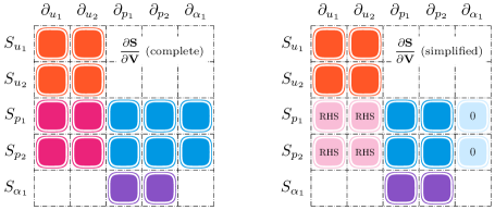
Figure 1: Visual comparison between the structure of the complete Jacobian matrix for the ODE system (6)–(10) and the proposed three-step simplified structure. The RHS label indicates dependencies that are accounted for as non-homogeneous terms in the pressure sub-system, while the zeros mark dependencies that are suppressed entirely.

Then the solution of the velocity sub-system can be immediately obtained as

$$u_{1}(t)=\frac{\lambda}{k}\,\left\{\frac{u_{1}^{0}}{\alpha_{2}\,\rho_{2}}+\frac{u_{2}^{0}}{\alpha_{1}\,\rho_{1}}+\frac{u_{1}^{0}-u_{2}^{0}}{\alpha_{1}\,\rho_{1}}\,\exp{\left[-k\,(t-t_{n})\right]}\right\},$$ (25)

$$u_{2}(t)=\frac{\lambda}{k}\,\left\{\frac{u_{1}^{0}}{\alpha_{2}\,\rho_{2}}+\frac{u_{2}^{0}}{\alpha_{1}\,\rho_{1}}+\frac{u_{2}^{0}-u_{1}^{0}}{\alpha_{2}\,\rho_{2}}\,\exp{\left[-k\,(t-t_{n})\right]}\right\},$$ (26)

with $k={1}/{\alpha_{1}\,\rho_{1}}+{1}/{\alpha_{2}\,\rho_{2}}$.

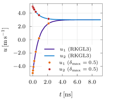
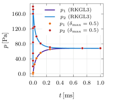
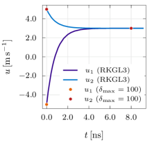
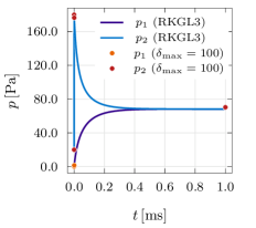
Figure 2: Time evolution of velocities and pressures for test problem A1. In the top frames the linearisation tolerance parameter is set as $\delta_{\mathrm{max}}=0.5$, employing 15 timesteps to reach the final time of $1.0\,\mathrm{ms}$, while in the bottom frames we impose an extremely loose tolerance $\delta_{\mathrm{max}}=100$, still showing good agreement with the reference solution but using only 4 timesteps for the full run.

In a second step, the pressure sub-system (8)–(9) is linearised as

$$\frac{\operatorname{d\!}{p_{1}}}{\vphantom{l^{l}}\operatorname{d\!}{t}}=k_{p}\,(p_{2}-p_{1})+k_{u}\,{(u_{I}-u_{1})}\,(u_{2}-u_{1}),$$ (27)

$$\frac{\operatorname{d\!}{p_{2}}}{\vphantom{l^{l}}\operatorname{d\!}{t}}=k_{p}\,(p_{1}-p_{2})+k_{u}\,{(u_{I}-u_{2})}\,(u_{1}-u_{2}),$$ (28)

where $k_{p}$ and $k_{u}$ are constant coefficients directly obtained from equations (8)–(9). This way, at the cost of suppressing the dependence on $\alpha_{1}$ in the Jacobian of the pressure sub-system, the homogeneous part of equations (27)–(28) has the same simple structure found in the velocity sub-system, with the addition of a non-homogeneous term, which is known, as $u_{1}(t)$ and $u_{2}(t)$ already have been computed. The solution can again be evaluated using standard scalar exponential functions, which are fast and robust, compared to matrix exponentials and especially so, because one no longer needs to perform the inversion of the Jacobian matrix of the full system.

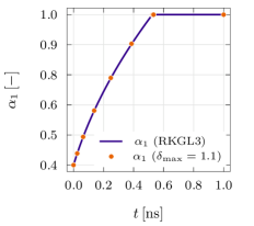
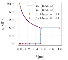
Figure 3: Time evolution of volume fraction and pressure for test problem A2. The solution is well captured in 11 timesteps, using a linearisation tolerance $\delta_{\mathrm{max}}=1.1$.

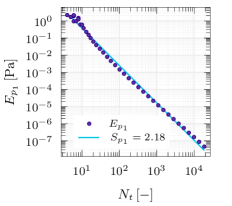
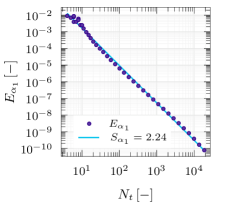
Figure 4: Convergence results relative to 40 runs of test problem A1. On the bilogarithmic plane, the slopes of the regression lines are $S_{p_{1}}=2.18$ and $S_{\alpha_{1}}=2.24$ for the variables $p_{1}$ and $\alpha_{1}$ respectively, indicating second order convergence.

Finally, the solution to equation (10) can be integrated analytically from the expressions of $p_{1}(t)$ and $p_{2}(t)$. Full coupling of the system is restored in the successive iterations by recomputing the constant coefficients $k_{p}$ and $k_{u}$ using an updated midpoint value for $\alpha_{1}$. See Figure 1 for a graphical description of the proposed simplified solution structure.

4 Test problems

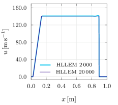
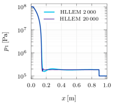
Figure 5: Solution of test Problem RP1 on two uniform meshes of 2 000 cells and 20 000 cells respectively, showing convergence with respect to mesh refinement.

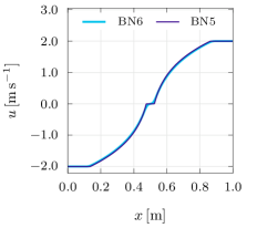
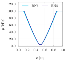
Figure 6: Solution of test Problem RP2 computed from the six-equation Baer–Nunziato model (BN6) with stiff relaxation, compared with the five-equation Kapila model (BN5), showing convergence to the limit reduced model.

We provide validation of the proposed method first by computing solutions to the ODE system (6)–(10) and comparing the results with a reference solution obtained from a sixth order, fully implicit, Runge–Kutta–Gauss–Legendre method butcher1964 (labeled RKGL3) employing adaptive timestepping (test problems A1 and A2, Figures 2 and 3). Furthermore, test problem A1 is employed also for carrying out a convergence study of the scheme (Figure 4), showing that second order convergence is easily achieved. The initial data for the ODE tests are, for test A1,

$$u_{1}^{0}=-5\,\mathrm{m\,s^{-1}},\ \ u_{2}^{0}=5\,\mathrm{m\,s^{-1}},\ \ p_{1}^{0}=0.1\,\mathrm{Pa},\ \ p_{2}^{0}=20\,\mathrm{Pa},\ \ \alpha_{1}^{0}=0.9,$$ (29)

while for test A2,

$$u_{1}^{0}=0\,\mathrm{m\,s^{-1}},\ \ u_{2}^{0}=0\,\mathrm{m\,s^{-1}},\ \ p_{1}^{0}=2.0\times 10^{8}\,\mathrm{Pa},\ \ p_{2}^{0}=1\,\mathrm{Pa},\ \ \alpha_{1}^{0}=0.4.$$ (30)

The parametric data are, for test A1,

$$\alpha_{1}\,\rho_{1}=1.0\,\mathrm{kg\,m^{-3}},\ \ \alpha_{2}\,\rho_{2}=4.0\,\mathrm{kg\,m^{-3}},\ \ \gamma_{1}=6,\ \ \gamma_{2}=1.4,$$ (31)

$$\Pi_{1}=0\,\mathrm{Pa},\ \ \Pi_{2}=0\,\mathrm{Pa},\ \ \lambda=10^{9}\,\mathrm{kg\,m^{-1}\,s^{-1}},\ \ \nu=10\,\mathrm{Pa^{-1}\,s^{-1}}.$$

and for test A2,

$$\alpha_{1}\,\rho_{1}=780.0\,\mathrm{kg\,m^{-3}},\ \ \alpha_{2}\,\rho_{2}=0.22\,\mathrm{kg\,m^{-3}},\ \ \gamma_{1}=6,\ \ \gamma_{2}=1.4,$$ (32)

$$\Pi_{1}=100\,\mathrm{Pa},\ \ \Pi_{2}=0\,\mathrm{Pa},\ \ \lambda=10^{9}\,\mathrm{kg\,m^{-1}\,s^{-1}},\ \ \nu=10\,\mathrm{Pa^{-1}\,s^{-1}}.$$

Then, we show an application of the method in the solution of the mixture-energy-consistent formulation of the six-equation reduced Baer–Nunziato model forwarded in pelanti . For these simulations the interface pressure is computed as

$$p_{I}=\frac{Z_{2}\,p_{1}+Z_{1}\,p_{2}}{Z_{1}+Z_{2}},\quad\text{with}\quad Z_{1}=\rho_{1}\,a_{1}\ \text{and}\ Z_{2}=\rho_{2}\,a_{2}.$$ (33)

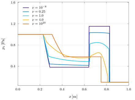
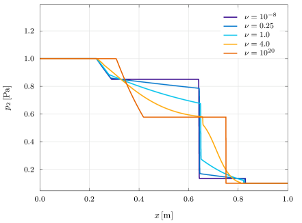
Figure 7: Behaviour of the pressure variables in RP3 with several values of $\nu$. It is clear that, in the stiff regime ($\nu=10^{20}\,\mathrm{Pa^{-1}\,s^{-1}}$), $p_{1}$ and $p_{2}$ converge to the same value, while they evolve in a completely distinct fashion if relaxation is set to act on longer timescales.

The first two shock-tube problems (from cavitation_shocktube ; pelanti ), show that the method is able to deal with very stiff ($\nu=10^{20}\,\mathrm{Pa^{-1}\,s^{-1}}$) sources, and in particular in Figure 5 (RP1, a liquid-vapour dodecane shock tube featuring a strong right-moving shockwave) we show mesh convergence of the solution by comparing two runs, both employing the HLLEM Riemann solver proposed in hllem , on two different meshes consisting of 2 000 uniform control volumes and 20 000 control volumes respectively, with a computational domain delimited by $x\in[0\,\mathrm{m},1\,\mathrm{m}]$. In Figure 6 (RP2, two diverging rarefaction waves in liquid water) we then show that, with very stiff relaxation ($\nu=10^{20}\,\mathrm{Pa^{-1}\,s^{-1}}$), the solution matches the one computed by solving directly the five-equation instantaneous equilibrium model kapila , again using a mesh consisting of 2 000 uniform cells for the six-equation model and a mesh of 20 000 uniform cells for the reference solution, and in particular, rarefaction waves propagate at the same speed for both models. All tests are run using a second order path-conservative MUSCL-Hancock scheme with $k_{\mathrm{CFL}}=0.95$. The first Riemann Problem (RP1) is set up with uniform liquid and vapour densities $\rho_{1}^{\mathrm{L}}=\rho_{1}^{\mathrm{R}}=500\,\mathrm{kg\,m^{-1}\,s^{-1}}$ and $\rho_{2}^{\mathrm{L}}=\rho_{2}^{\mathrm{L}}=2.0\,\mathrm{kg\,m^{-3}}$, uniform velocity $u^{\mathrm{L}}=u^{\mathrm{R}}=0\,\mathrm{m\,s^{-1}}$, a jump in pressure given by $p_{1}^{\mathrm{L}}=p_{2}^{\mathrm{L}}=100\,\mathrm{MPa}$, $p_{1}^{\mathrm{R}}=p_{2}^{\mathrm{R}}=100\,\mathrm{kPa}$, almost pure liquid on the left side of the initial discontinuity ($\alpha_{1}^{\mathrm{L}}=1-10^{-8}$), and almost pure vapor on the right side ($\alpha_{1}^{\mathrm{R}}=10^{-8}$). The discontinuity is initially found at $x=0.75\,\mathrm{m}$, and the end time is $t_{\mathrm{end}}=473\,\mathrm{\mu s}$. The parameters of the stiffened gas EOS are $\gamma_{1}=2.35$, $\gamma_{2}=1.025$, $\Pi_{1}=400\,\mathrm{MPa}$, $\Pi_{2}=0$.

The second Riemann Problem (RP2) is initialised with constant liquid and vapour densities $\rho_{1}^{\mathrm{L}}=\rho_{1}^{\mathrm{R}}=1150\,\mathrm{kg\,m^{-1}\,s^{-1}}$, $\rho_{2}^{\mathrm{L}}=\rho_{2}^{\mathrm{L}}=0.63\,\mathrm{kg\,m^{-3}}$, constant pressure $p_{1}^{\mathrm{L}}=p_{2}^{\mathrm{L}}=p_{1}^{\mathrm{R}}=p_{2}^{\mathrm{R}}=100\,\mathrm{kPa}$, constant liquid volume fraction $\alpha_{1}^{\mathrm{L}}=\alpha_{1}^{\mathrm{R}}=0.99$, and a jump in velocity (initially located at $x=0.5\,\mathrm{m}$) such that $u^{\mathrm{L}}=-2.0\,\mathrm{m\,s^{-1}}$ and $u^{\mathrm{R}}=2.0\,\mathrm{m\,s^{-1}}$. The final time is $t_{\mathrm{end}}=3.2\,\mathrm{ms}$ and for this test the parameters of the equation of state $\gamma_{1}=2.35$, $\gamma_{2}=1.43$, $\Pi_{1}=1\,\mathrm{GPa}$, $\Pi_{2}=0$.

Finally, in Figure 7 we show the behaviour of the solution of a third Riemann problem (RP3) with several different values of the pressure relaxation parameter $\nu$ (ranging from $10^{-8}\,\mathrm{Pa^{-1}\,s^{-1}}$ to $10^{20}\,\mathrm{Pa^{-1}\,s^{-1}}$), highlighting the vast range of solution structures that can be obtained not only with stiff relaxation (the pressure profiles $p_{1}$ and $p_{2}$ coincide) or in total absence of it, but also with finite values of the relaxation time scale. For RP3, the initial data on the left are

$$\rho_{1}^{\mathrm{L}}=1.0\,\mathrm{kg\,m^{-1}\,s^{-1}},\quad\rho_{2}^{\mathrm{L}}=0.2\,\mathrm{kg\,m^{-3}},\quad u^{\mathrm{L}}=0.0\,\mathrm{m\,s^{-1}},$$ (34)

$$p_{1}^{\mathrm{L}}=1.0\,\mathrm{Pa},\quad p_{2}^{\mathrm{L}}=1.0\,\mathrm{Pa},\quad\alpha_{1}^{\mathrm{L}}=0.55,$$

while on the right one has

$$\rho_{1}^{\mathrm{R}}=0.125\,\mathrm{kg\,m^{-3}},\quad\rho_{2}^{\mathrm{R}}=2.0\,\mathrm{kg\,m^{-3}},\quad u^{\mathrm{R}}=0.0\,\mathrm{m\,s^{-1}},$$ (35)

$$p_{1}^{\mathrm{R}}=0.1\,\mathrm{Pa},\quad p_{2}^{\mathrm{R}}=0.1\,\mathrm{Pa},\quad\alpha_{1}^{\mathrm{R}}=0.45.$$

The initial jump is located at $x=0.6\,\mathrm{m}$, the domain is $x\in[0\,\mathrm{m},\ 1\,\mathrm{m}]$ and the final time is $t_{\mathrm{end}}=0.15\,\mathrm{s}$. The parameters of the stiffened gas EOS are $\gamma_{1}=2.0$, $\gamma_{2}=1.4$, $\Pi_{1}=2.0\,\mathrm{Pa}$, $\Pi_{2}=0.0\,\mathrm{Pa}$.

5 Conclusions

We presented a technique for integrating ordinary differential equations associated with stiff relaxation sources and promising results have been shown for a set of test problems. The method can efficiently resolve very abrupt variations in the solution and adapt to multiple timescales. A key feature of the algorithm is that it can avoid delicate linear algebra operations entirely, thus improving the robustness of the scheme. Future applications will include liquid-gas and liquid-solid phase transition, strain relaxation for nonlinear elasticity gpr and the computation of material failure in elasto-plastic and brittle solids.

References

• [1] A. H. Al-Mohy and N. J. Higham. A new scaling and squaring algorithm for the matrix exponential. SIAM Journal on Matrix Analysis and Applications, 31(3):970–989, 2009.
• [2] A. H. Al-Mohy and N. J. Higham. Computing the action of the matrix exponential, with an application to exponential integrators. SIAM Journal on Scientific Computing, 33(2):488–511, 2011.
• [3] M. R. Baer and J. W. Nunziato. A two-phase mixture theory for the deflagration-to-detonation transition (DDT) in reactive granular materials. International Journal of Multiphase Flow, 12(6):861–889, 1986.
• [4] J. C. Butcher. Implicit Runge–Kutta processes. Mathematics of Computation, 18(85):50–64, 1964.
• [5] M. Castro, J. M. Gallardo, and C. Parés. High order finite volume schemes based on reconstruction of states for solving hyperbolic systems with nonconservative products. Applications to shallow-water systems. Mathematics of Computation, 75(255):1103–1134, 2006.
• [6] J. Certaine. The solution of ordinary differential equations with large time constants. Mathematical Methods for Digital Computers, pages 128–132, 1960.
• [7] M. Dumbser and D. S. Balsara. A new efficient formulation of the HLLEM Riemann solver for general conservative and non-conservative hyperbolic systems. Journal of Computational Physics, 304(C):275–319, 2016.
• [8] M. Dumbser, I. Peshkov, E. Romenski, and O. Zanotti. High order ader schemes for a unified first order hyperbolic formulation of continuum mechanics: Viscous heat-conducting fluids and elastic solids. Journal of Computational Physics, 314:824–862, 2016.
• [9] N. J. Higham. The scaling and squaring method for the matrix exponential revisited. SIAM Journal on Matrix Analysis and Applications, 26(4):1179–1193, 2005.
• [10] A. K. Kapila, R. Menikoff, J. B. Bdzil, S. F. Son, and D. S. Stewart. Two-phase modeling of deflagration-to-detonation transition in granular materials: Reduced equations. Physics of Fluids, 13(10):3002–3024, 2001.
• [11] C. Parès. Numerical methods for nonconservative hyperbolic systems: a theoretical framework. SIAM Journal on Numerical Analysis, 44(1):300–321, 2006.
• [12] M. Pelanti and K.-M. Shyue. A mixture-energy-consistent six-equation two-phase numerical model for fluids with interfaces, cavitation and evaporation waves. Journal of Computational Physics, 259:331–357, 2014.
• [13] D. A. Pope. An exponential method of numerical integration of ordinary differential equations. Communications of the ACM, 6(8):491–493, 1963.
• [14] R. Saurel, F. Petitpas, and R. A. Berry. Simple and efficient relaxation methods for interfaces separating compressible fluids, cavitating flows and shocks in multiphase mixtures. Journal of Computational Physics, 228(5):1678–1712, 2009.
• [15] Richard Saurel, Fabien Petitpas, and Remi Abgrall. Modelling phase transition in metastable liquids: application to cavitating and flashing flows. Journal of Fluid Mechanics, 607:313––350, 2008.
• [16] G. Strang. On the Construction and Comparison of Difference Schemes. SIAM Journal on Numerical Analysis, 5:506–517, 1968.
• [17] E. F. Toro. Riemann Solvers and Numerical Methods for Fluid Dynamics. A Practical Introduction, Third edition. Springer-Verlag, Berlin, 2009.
• [18] B. van Leer. Towards the ultimate conservative difference scheme. V. A second-order sequel to Godunov’s method. Journal of Computational Physics, 32(1):101–136, 1979.
• [19] N. N. Yanenko. The method of fractional steps. Springer, 1971.