Hadroproduction of scalar $P$-wave quarkonia
in the light-front $k_{T}$-factorization approach

Abstract

In this work, we present a thorough analysis of scalar $P$-wave $\chi_{Q0}$, $Q=c,b$ quarkonia electromagnetic form factors for the $\gamma^{*}\gamma^{*}\to\chi_{Q0}$ couplings, as well as their hadroproduction observables in $k_{\perp}$-factorisation using the light-front potential approach for the quarkonium wave function. The electromagnetic form factors are presented as functions of photon virtualities. We discuss the role of the Melosh spin-rotation and relativistic corrections estimated by comparing our results with those in the standard nonrelativistic QCD (NRQCD) approach. Theoretical uncertainties of our approach are found by performing the analysis with two different unintegrated gluon densities and with five distinct models of the $Q\bar{Q}$ interaction potentials consistent with the meson spectra. The results for the rapidity and transverse momentum distributions of $\chi_{Q0}$ produced in high-energy $pp$ collisions at $\sqrt{s}=13\,\rm{TeV}$ are shown.

I Introduction

The production of quarkonia in hadronic collisions continues to attract a lot of interest Lansberg:2019adr ; Chisholm:2014sca ; Belyaev:2015lkw ; Baranov:2019lhm . Different approaches were used in the past, for the case of $\chi_{c},\chi_{b}$ production, see e.g. Hagler:2000dd ; Kniehl:2006sk ; Baranov:2015yea ; CS2018 ; Likhoded:2012hw ; Likhoded:2014kfa ; Diakonov:2012vb ; Boer:2012bt . Here, we continue our investigation BPSS2019 ; BGPSS2019 of quarkonia production observables in the framework of the $k_{\perp}$-factorisation approach Gribov:1984tu ; Catani:1990xk ; Collins:1991ty in the color-singlet formulation employing the light-front quarkonia wave functions. The previous works in Refs. Hagler:2000dd ; Kniehl:2006sk ; Baranov:2015yea ; CS2018 have observed that in the $k_{\perp}$-factorisation approach the color-singlet mechanism dominates in the quarkonia production. At the next natural step we pursue in this direction, it is instructive to explore the role of relativistic corrections and the shape of the quarkonia wave function in the associated observables.

In our recent study BPSS2019 ; BGPSS2019 we discussed inclusive production of pseudoscalar $\eta_{c}(1S,2S)$ charmonia in proton-proton collisions. We explicitly calculated the corresponding electromagnetic $\gamma^{*}+\gamma^{*}\to\eta_{c}(1S,2S)$ form factors as functions of photon virtualities. Similar form factors were calculated also for the $g^{*}+g^{*}\to\eta_{c}(1S,2S)$ matrix element that was used in the $k_{T}$-factorization formula for differential hadroproduction cross section. We have shown there that inclusion of both form factors in such an approach is essential. In our calculations, we adopted the color-singlet model, which treats the quarkonium as a two-body bound state of heavy quark and antiquark.

Such a formalism was used previously for the production of $\chi_{cJ}$ ($J=0,1,2$) quarkonia (see e.g. Ref. CS2018 and references therein), and a relatively good agreement with data was obtained in the $k_{T}$-factorization approach with an unintegrated gluon distribution (UGD), which effectively includes higher-order corrections. These previous calculations were done within the nonrelativistic QCD (NRQCD) approach.

In this work, we discuss production of the lowest $P$-wave scalar state for both $c\bar{c}$ and $b\bar{b}$ systems, $\chi_{Q0}$, $Q=c,b$, in the same approach which we dubbed at the light-front $k_{\perp}$-factorisation. As will be discussed in detail below, the situation with scalar $\chi_{c0}$ production is a bit more complicated than that for the pseudoscalar quarkonia. The leading-order partonic subprocess at high energies is the off-shell gluon-gluon fusion, $g^{*}+g^{*}\to\chi_{Q0}$. The main ingredient of such a subprocess is the off-shell matrix element written in terms of two independent form factors. Here we go beyond the NRQCD approach and present a similar analysis of $\chi_{Q0}$ form factors and hadroproduction as was done earlier for pseudoscalar ($S$-wave) charmonia. We will present the corresponding form factors, compare the new results to those obtained in NRQCD approaches and make predictions for the $pp\to\chi_{Q0}$ reactions at the LHC energies.

The paper is organised as follows. In Sec. II, we recapitulate the main details of the $k_{\perp}$-factorisation formalism. In Sec. III we derive the off-shell matrix element expressed in terms of two independent form factors written in terms of light-front quarkonia wave functions. These form factors can be related to the standard electromagnetic transition form factors, which encode the helicity dependence of the virtual-photon fusion amplitudes. We derive the relevant expressions in Sec. IV. We then turn to numerical results, presenting the light front wave functions and radiative decay widths in Sec. V. In Sec. VI we present our results for the electromagnetic form factors. Our results for the transverse momentum and rapidity distributions of $\chi_{c0}$ and $\chi_{b0}$ mesons are shown in Sec. VII. In Sec. VIII we conclude.

II $k_{T}$-factorization for inclusive hadroproduction

Let us briefly recapitulate the $k_{T}$-factorization formalism we use in this work. The leading process is the gluon-gluon fusion into the color-singlet heavy quark pair. Gluons carry transverse momenta, and their four momenta are written as ($\sqrt{s}$ is the $pp$ center-of-mass energy, and we use the lightcone components of four-vectors $a=(a_{+},a_{-},\mbox{\boldmath$a$})\,,\,a^{2}=2a_{+}a_{-}-\mbox{\boldmath$a$}^{2}$):

$$q_{1}=(q_{1+},0,\mbox{\boldmath$q$}_{1})\,,\,q_{2}=(0,q_{2-},\mbox{\boldmath$q$}_{2})\,,$$ (1)

with

$$q_{1+}=x_{1}\sqrt{s\over 2}\,,\,q_{2-}=x_{2}\sqrt{s\over 2}\,.$$ (2)

An important distinction from the collinear approach is that the gluon momenta are (spacelike) off-shell, $q_{i}^{2}=-\mbox{\boldmath$q$}_{i}^{2},i=1,2$. Our starting point is the inclusive cross section for the $2\to 1$ gluon-gluon fusion mode obtained from

$$d\sigma=\int{dx_{1}\over x_{1}}\int{d^{2}\mbox{\boldmath$q$}_{1}\over\pi\mbox{\boldmath$q$}_{1}^{2}}{\cal{F}}(x_{1},\mbox{\boldmath$q$}_{1}^{2},\mu_{F}^{2})\int{dx_{2}\over x_{2}}\int{d^{2}\mbox{\boldmath$q$}_{2}\over\pi\mbox{\boldmath$q$}_{2}^{2}}{\cal{F}}(x_{2},\mbox{\boldmath$q$}_{2}^{2},\mu_{F}^{2}){1\over 2x_{1}x_{2}s}\overline{|{\cal{M}}|^{2}}\,d\Phi(2\to 1).$$

Here the unintegrated gluon distributions are normalized such that the collinear glue is given by

$$xg(x,\mu_{F}^{2})=\int^{\mu_{F}^{2}}{d\mbox{\boldmath$q$}^{2}\over\mbox{\boldmath$q$}^{2}}{\cal{F}}(x,\mbox{\boldmath$q$}^{2},\mu_{F}^{2})\,,$$ (4)

where from now on we will no longer show the dependence on the factorization scale $\mu_{F}^{2}$ explicitly. Let us denote the four-momentum of $\chi$ meson by $p$ and parametrize it in light-cone coordinates as

$$p=(p_{+},p_{-},\mbox{\boldmath$p$})=\Big{(}{m_{T}\over\sqrt{2}}e^{y},{m_{T}\over\sqrt{2}}e^{-y},\mbox{\boldmath$p$}\Big{)}\,,\qquad m_{T}=\sqrt{\mbox{\boldmath$p$}^{2}+M_{\chi}^{2}}.$$ (5)

Here $M_{\chi}$ is the mass of the $\chi_{Q0}$-meson, $p$ is its transverse momentum, and $y$ its rapidity in the $pp$ c.m. frame. The phase-space element is

$$d\Phi(2\to 1) = (2\pi)^{4}\delta^{(4)}(q_{1}+q_{2}-p)\,{d^{4}p\over(2\pi)^{3}}\delta(p^{2}-M_{\chi}^{2})$$ (6)

$$= {2\pi\over s}\delta(x_{1}-{m_{T}\over\sqrt{s}}e^{y})\delta(x_{2}-{m_{T}\over\sqrt{s}}e^{-y})\delta^{(2)}(\mbox{\boldmath$q$}_{1}+\mbox{\boldmath$q$}_{2}-\mbox{\boldmath$p$})\,dy\,d^{2}\mbox{\boldmath$p$}\,.$$

We therefore obtain for the inclusive cross section

$${d\sigma\over dyd^{2}\mbox{\boldmath$p$}}=\int{d^{2}\mbox{\boldmath$q$}_{1}\over\pi\mbox{\boldmath$q$}_{1}^{2}}{\cal{F}}(x_{1},\mbox{\boldmath$q$}_{1}^{2})\int{d^{2}\mbox{\boldmath$q$}_{2}\over\pi\mbox{\boldmath$q$}_{2}^{2}}{\cal{F}}(x_{2},\mbox{\boldmath$q$}_{2}^{2})\,\delta^{(2)}(\mbox{\boldmath$q$}_{1}+\mbox{\boldmath$q$}_{2}-\mbox{\boldmath$p$})\,{\pi\over(x_{1}x_{2}s)^{2}}\overline{|{\cal{M}}|^{2}},$$ (7)

where the momentum fractions of gluons are fixed as $x_{1,2}=m_{T}\exp(\pm y)/\sqrt{s}$. The off-shell matrix element is written in terms of the Feynman amplitude as (we restore the color-indices):

$${\cal{M}}^{ab}={q_{1\perp}^{\mu}q_{2\perp}^{\nu}\over|\mbox{\boldmath$q$}_{1}||\mbox{\boldmath$q$}_{2}|}{\cal{M}}^{ab}_{\mu\nu}={q_{1+}q_{2-}\over|\mbox{\boldmath$q$}_{1}||\mbox{\boldmath$q$}_{2}|}n^{+}_{\mu}n^{-}_{\nu}{\cal{M}}^{ab}_{\mu\nu}={x_{1}x_{2}s\over 2|\mbox{\boldmath$q$}_{1}||\mbox{\boldmath$q$}_{2}|}n^{+}_{\mu}n^{-}_{\nu}{\cal{M}}^{ab}_{\mu\nu}\,.$$ (8)

III $k_{T}$-factorization element for final state $Q\bar{Q}$

Let us introduce the reduced amplitude

$${\cal T}_{\mu\nu}\equiv{1\over 4\pi\alpha_{\rm em}e_{Q}^{2}}\,\int{dzd^{2}\mbox{\boldmath$k$}\over z(1-z)16\pi^{3}}\sum_{\lambda,\bar{\lambda}}\Psi^{*}_{\lambda\bar{\lambda}}(z,\mbox{\boldmath$k$}){\cal M}_{\mu\nu}^{\lambda\bar{\lambda}}(\gamma^{*}\gamma^{*}\to Q_{\lambda}(zP_{+},\mbox{\boldmath$p$}_{Q})\bar{Q}_{\bar{\lambda}}((1-z)P_{+},\mbox{\boldmath$p$}_{\bar{Q}})\,.$$

Here the transverse momenta of quark and antiquark are

$$\mbox{\boldmath$p$}_{Q}=\mbox{\boldmath$k$}+z\mbox{\boldmath$P$}\,,\qquad\mbox{\boldmath$p$}_{\bar{Q}}=-\mbox{\boldmath$k$}+(1-z)\mbox{\boldmath$P$}\,.$$ (10)

The photon-photon fusion and gluon-gluon fusion amplitudes are proportional to the reduced amplitude as follows:

$${\cal M}_{\mu\nu}(\gamma^{*}\gamma^{*}\to\chi_{Q0}(P_{+},\mbox{\boldmath$P$})) = 4\pi\alpha_{\rm em}e_{Q}^{2}{{\mbox{\rm Tr}}[\openone]\over\sqrt{N_{c}}}\,{\cal T}_{\mu\nu}=4\pi\alpha_{\rm em}e_{Q}^{2}\sqrt{N_{c}}\,{\cal T}_{\mu\nu}\,,$$

$${\cal M}^{ab}_{\mu\nu}(g^{*}g^{*}\to\chi_{Q0}(P_{+},\mbox{\boldmath$P$})) = 4\pi\alpha_{s}{{\mbox{\rm Tr}}[t^{a}t^{b}]\over\sqrt{N_{c}}}\,{\cal T}_{\mu\nu}={2\pi\alpha_{s}\over\sqrt{N_{c}}}\,\delta^{ab}{\cal T}_{\mu\nu}\,.$$ (11)

For the purpose of $k_{T}$-factorization it is most convenient to use the contraction of the gluon-fusion amplitude with light-cone vectors $n_{\mu}^{\pm}$. Using the standard covariant Feynman rules, we can obtain the reduced amplitude ${\cal T}=n^{+\mu}n^{-\nu}{\cal T}_{\mu\nu}$ as

$${\cal T} = (-2)\int{dzd^{2}\mbox{\boldmath$k$}\over\sqrt{z(1-z)}16\pi^{3}}$$ (12)

$$\times \Big{\{}-m_{Q}\Big{[}{1\over\mbox{\boldmath$l$}_{A}^{2}+\varepsilon^{2}}-{1\over\mbox{\boldmath$l$}_{B}^{2}+\varepsilon^{2}}\Big{]}\Big{(}\sqrt{2}(\mbox{\boldmath$e$}(-)\mbox{\boldmath$q$}_{1})\Psi^{*}_{++}(z,\mbox{\boldmath$k$})+\sqrt{2}(\mbox{\boldmath$e$}(+)\mbox{\boldmath$q$}_{1})\Psi^{*}_{--}(z,\mbox{\boldmath$k$})\Big{)}$$

$$+ \Big{(}2z(1-z)\mbox{\boldmath$q$}_{1}^{2}+(1-2z)(\mbox{\boldmath$k$}\mbox{\boldmath$q$}_{1})\Big{)}\Big{[}{1\over\mbox{\boldmath$l$}_{A}^{2}+\varepsilon^{2}}-{1\over\mbox{\boldmath$l$}_{B}^{2}+\varepsilon^{2}}\Big{]}\Big{(}\Psi^{*}_{+-}(z,\mbox{\boldmath$k$})+\Psi^{*}_{-+}(z,\mbox{\boldmath$k$})\Big{)}$$

$$- (1-2z)(\mbox{\boldmath$q$}_{1}\mbox{\boldmath$q$}_{2})\Big{[}{1-z\over\mbox{\boldmath$l$}_{A}^{2}+\varepsilon^{2}}+{z\over\mbox{\boldmath$l$}_{B}^{2}+\varepsilon^{2}}\Big{]}\Big{(}\Psi^{*}_{+-}(z,\mbox{\boldmath$k$})+\Psi^{*}_{-+}(z,\mbox{\boldmath$k$})\Big{)}\Big{\}}\;.$$

Here we have introduced the shorthand notation

$$\varepsilon^{2} = z(1-z)\mbox{\boldmath$q$}_{1}^{2}+m_{Q}^{2}\,,\qquad\mbox{\boldmath$l$}_{A}=\mbox{\boldmath$k$}-(1-z)\mbox{\boldmath$q$}_{2}\,,\qquad\mbox{\boldmath$l$}_{B}=\mbox{\boldmath$k$}+z\mbox{\boldmath$q$}_{2}\,.$$ (13)

We have also made use of the fact, that for the scalar meson

$$\Psi^{*}_{+-}(z,\mbox{\boldmath$k$})-\Psi^{*}_{-+}(z,\mbox{\boldmath$k$}) = 0.$$ (14)

We have collected the necessary information on the light-front wave function $\Psi_{\lambda\bar{\lambda}}(z,\mbox{\boldmath$k$})$ in Appendix A. Inserting the identities which follow from Eq.(75):

$$\sqrt{2}(\mbox{\boldmath$e$}(-)\mbox{\boldmath$q$}_{1})\Psi^{*}_{++}(z,\mbox{\boldmath$k$})+\sqrt{2}(\mbox{\boldmath$e$}(+)\mbox{\boldmath$q$}_{1})\Psi^{*}_{--}(z,\mbox{\boldmath$k$}) = {2(\mbox{\boldmath$q$}_{1}\mbox{\boldmath$k$})\over\sqrt{z(1-z)}}\psi(z,\mbox{\boldmath$k$})\,,$$

$$\Psi^{*}_{+-}(z,\mbox{\boldmath$k$})+\Psi^{*}_{-+}(z,\mbox{\boldmath$k$}) = {2m_{Q}(1-2z)\over\sqrt{z(1-z)}}\psi(z,\mbox{\boldmath$k$})\,,$$ (15)

we can simplify the amplitude further to read

$${\cal T} = (-4m_{Q})\int{dzd^{2}\mbox{\boldmath$k$}\over z(1-z)16\pi^{3}}\psi(z,\mbox{\boldmath$k$})\Big{\{}2z(1-z)(1-2z)\mbox{\boldmath$q$}_{1}^{2}\Big{[}{1\over\mbox{\boldmath$l$}_{A}^{2}+\varepsilon^{2}}-{1\over\mbox{\boldmath$l$}_{B}^{2}+\varepsilon^{2}}\Big{]}$$ (16)

$$- 4z(1-z)(\mbox{\boldmath$k$}\mbox{\boldmath$q$}_{1})\Big{[}{1\over\mbox{\boldmath$l$}_{A}^{2}+\varepsilon^{2}}-{1\over\mbox{\boldmath$l$}_{B}^{2}+\varepsilon^{2}}\Big{]}-(1-2z)^{2}(\mbox{\boldmath$q$}_{1}\mbox{\boldmath$q$}_{2})\Big{[}{1-z\over\mbox{\boldmath$l$}_{A}^{2}+\varepsilon^{2}}+{z\over\mbox{\boldmath$l$}_{B}^{2}+\varepsilon^{2}}\Big{]}\Big{\}}\;.$$

There now emerge two independent form factors $G_{1,2}(\mbox{\boldmath$q$}_{1}^{2},\mbox{\boldmath$q$}_{2}^{2})$:

$${\cal T}=|\mbox{\boldmath$q$}_{1}||\mbox{\boldmath$q$}_{2}|G_{1}(\mbox{\boldmath$q$}_{1}^{2},\mbox{\boldmath$q$}_{2}^{2})+(\mbox{\boldmath$q$}_{1}\cdot\mbox{\boldmath$q$}_{2})G_{2}(\mbox{\boldmath$q$}_{1}^{2},\mbox{\boldmath$q$}_{2}^{2})\,.$$ (17)

The form factors $G_{1,2}(\mbox{\boldmath$q$}_{1}^{2},\mbox{\boldmath$q$}_{2}^{2})$ have the integral representations

$$G_{1}(\mbox{\boldmath$q$}_{1}^{2},\mbox{\boldmath$q$}_{2}^{2}) = |\mbox{\boldmath$q$}_{1}||\mbox{\boldmath$q$}_{2}|\,{4m_{Q}\over\mbox{\boldmath$q$}_{2}^{2}}\int{dzd^{2}\mbox{\boldmath$k$}\over z(1-z)16\pi^{3}}\psi(z,\mbox{\boldmath$k$})\,2z(1-z)(2z-1)\Big{[}{1\over\mbox{\boldmath$l$}_{A}^{2}+\varepsilon^{2}}-{1\over\mbox{\boldmath$l$}_{B}^{2}+\varepsilon^{2}}\Big{]}$$

$$G_{2}(\mbox{\boldmath$q$}_{1}^{2},\mbox{\boldmath$q$}_{2}^{2}) = 4m_{Q}\int{dzd^{2}\mbox{\boldmath$k$}\over z(1-z)16\pi^{3}}\psi(z,\mbox{\boldmath$k$})\Big{[}{1-z\over\mbox{\boldmath$l$}_{A}^{2}+\varepsilon^{2}}+{z\over\mbox{\boldmath$l$}_{B}^{2}+\varepsilon^{2}}\Big{]}$$ (18)

$$+ {4m_{Q}\over\mbox{\boldmath$q$}_{2}^{2}}\int{dzd^{2}\mbox{\boldmath$k$}\over z(1-z)16\pi^{3}}\psi(z,\mbox{\boldmath$k$})4z(1-z)\Big{[}{\mbox{\boldmath$q$}_{2}\cdot\mbox{\boldmath$l$}_{A}\over\mbox{\boldmath$l$}_{A}^{2}+\varepsilon^{2}}-{\mbox{\boldmath$q$}_{2}\cdot\mbox{\boldmath$l$}_{B}\over\mbox{\boldmath$l$}_{B}^{2}+\varepsilon^{2}}\Big{]}\,.$$

We explain in Appendix A how the light-front radial WF $\psi(z,\mbox{\boldmath$k$})$ can be obtained from the potential model WF using the Melosh-transform technique for the spin-orbit part Melosh:1974cu ; Jaus:1989au augmented by the Terent’ev prescription Terentev:1976jk .

Finally, the factorization formula for the hadroproduction process $pp\to\chi_{Q0}X$ reads as follows

$${d\sigma\over dyd^{2}\mbox{\boldmath$p$}} = \int{d^{2}\mbox{\boldmath$q$}_{1}\over\pi\mbox{\boldmath$q$}_{1}^{4}}{d^{2}\mbox{\boldmath$q$}_{2}\over\pi\mbox{\boldmath$q$}_{2}^{4}}\delta^{(2)}(\mbox{\boldmath$p$}-\mbox{\boldmath$q$}_{1}-\mbox{\boldmath$q$}_{2}){\cal F}(x_{1},\mbox{\boldmath$q$}_{1}){\cal F}(x_{2},\mbox{\boldmath$q$}_{2}){\pi\over 4(N_{c}^{2}-1)^{2}}\,\sum_{a,b}|{\cal M}^{ab}_{\mu\nu}n^{+}_{\mu}n^{-}_{\nu}|^{2}\,$$ (19)

$$= \int{d^{2}\mbox{\boldmath$q$}_{1}\over\pi\mbox{\boldmath$q$}_{1}^{4}}{d^{2}\mbox{\boldmath$q$}_{2}\over\pi\mbox{\boldmath$q$}_{2}^{4}}\delta^{(2)}(\mbox{\boldmath$p$}-\mbox{\boldmath$q$}_{1}-\mbox{\boldmath$q$}_{2}){\cal F}(x_{1},\mbox{\boldmath$q$}_{1}){\cal F}(x_{2},\mbox{\boldmath$q$}_{2}){\pi^{3}\alpha_{S}^{2}|{\cal T}|^{2}\over N_{c}(N_{c}^{2}-1)}\;$$

$$= \int{d^{2}\mbox{\boldmath$q$}_{1}\over\pi\mbox{\boldmath$q$}_{1}^{2}}{d^{2}\mbox{\boldmath$q$}_{2}\over\pi\mbox{\boldmath$q$}_{2}^{2}}\delta^{(2)}(\mbox{\boldmath$p$}-\mbox{\boldmath$q$}_{1}-\mbox{\boldmath$q$}_{2}){\cal F}(x_{1},\mbox{\boldmath$q$}_{1}){\cal F}(x_{2},\mbox{\boldmath$q$}_{2}){\pi^{3}\alpha_{S}^{2}\over N_{c}(N_{c}^{2}-1)}$$

$$\times \Big{(}G_{1}(\mbox{\boldmath$q$}_{1}^{2},\mbox{\boldmath$q$}_{2}^{2})+\cos(\phi_{1}-\phi_{2})G_{2}(\mbox{\boldmath$q$}_{1}^{2},\mbox{\boldmath$q$}_{2}^{2})\Big{)}^{2}\;,$$

with $\phi_{1,2}$ being the azimuthal angles of gluon transverse momenta $\mbox{\boldmath$q$}_{1,2}$. In our numerical calculations presented below, we set the factorization scale to $\mu_{F}^{2}=m_{T}^{2}$, and the QCD coupling constant squared in the differential cross section above is taken in the following form:

$$\alpha_{s}^{2}\to\alpha_{s}(\max{\{m_{T}^{2},\mbox{\boldmath$q$}_{1}^{2}\}})\alpha_{s}(\max{\{m_{T}^{2},\mbox{\boldmath$q$}_{2}^{2}\}})\;.$$ (20)

III.1 NRQCD limit

Let us now take the nonrelativistic (NR) limit. In this case, one should Taylor-expand around $z=1/2$ and $\mbox{\boldmath$k$}=0$. Let us introduce

$$z={1\over 2}+\xi\,,\qquad 1-z={1\over 2}-\xi\,.$$ (21)

We can see, that in zeroth order the form factors $G_{1},G_{2}$ vanish. To the first order in $\xi$ and $k$, we obtain

$${1\over\mbox{\boldmath$l$}_{A}^{2}+\varepsilon^{2}}-{1\over\mbox{\boldmath$l$}_{B}^{2}+\varepsilon^{2}}={2\over\mu^{4}}\Big{(}\xi\mbox{\boldmath$q$}_{2}^{2}+(\mbox{\boldmath$k$}\mbox{\boldmath$q$}_{2})\Big{)}\,,$$ (22)

with

$$\mu^{2}={1\over 4}\Big{(}\mbox{\boldmath$q$}_{1}^{2}+\mbox{\boldmath$q$}_{2}^{2}+4m_{c}^{2}\Big{)}\,.$$ (23)

In the NR limit, we also replace $2m_{Q}\to M_{\chi}$, and obtain for the two form factors

$$G_{1}(\mbox{\boldmath$q$}_{1}^{2},\mbox{\boldmath$q$}_{2}^{2}) = {|\mbox{\boldmath$q$}_{1}||\mbox{\boldmath$q$}_{2}|\over\mu^{4}}{4\over M_{\chi}}\,\int{dzd^{2}\mbox{\boldmath$k$}\over z(1-z)16\pi^{3}}\psi(z,\mbox{\boldmath$k$})\,\xi^{2}M_{\chi}^{2}\,,$$

$$G_{2}(\mbox{\boldmath$q$}_{1}^{2},\mbox{\boldmath$q$}_{2}^{2}) = {2\over\mu^{4}}{1\over M_{\chi}}\int{dzd^{2}\mbox{\boldmath$k$}\over z(1-z)16\pi^{3}}\psi(z,\mbox{\boldmath$k$})\Big{(}\mbox{\boldmath$k$}^{2}M_{\chi}^{2}+4\xi^{2}M_{\chi}^{2}\mu^{2}\Big{)}\,.$$ (24)

Now, again in the NR limit, we can replace $\xi M_{\chi}=k_{z}$, and substitute

$${dzd^{2}\mbox{\boldmath$k$}\over z(1-z)16\pi^{3}}\psi(z,\mbox{\boldmath$k$})\to{1\over 4\pi^{2}\sqrt{M_{\chi}}}{1\over 2\sqrt{2}}d^{3}k{u(k)\over k^{2}}\,.$$ (25)

Using the relation

$$\int_{0}^{\infty}dk\,k^{2}u(k)=3\sqrt{\pi\over 2}R^{\prime}(0)\,,$$ (26)

we see that both form factors are proportional to the first derivative of the radial wave function at the origin $R^{\prime}(0)$:

$$G_{1}(\mbox{\boldmath$q$}_{1}^{2},\mbox{\boldmath$q$}_{2}^{2}) = {2|\mbox{\boldmath$q$}_{1}||\mbox{\boldmath$q$}_{2}|\over\ [M_{\chi}^{2}+\mbox{\boldmath$q$}_{1}^{2}+\mbox{\boldmath$q$}_{2}^{2}]^{2}}\,\lambda\,,\qquad G_{2}(\mbox{\boldmath$q$}_{1}^{2},\mbox{\boldmath$q$}_{2}^{2})={3M_{\chi}^{2}+\mbox{\boldmath$q$}_{1}^{2}+\mbox{\boldmath$q$}_{2}^{2}\over[M_{\chi}^{2}+\mbox{\boldmath$q$}_{1}^{2}+\mbox{\boldmath$q$}_{2}^{2}]^{2}}\,\lambda\,.$$ (27)

Here we introduced the short-hand notation

$$\lambda={8\over\sqrt{\pi}}{R^{\prime}(0)\over M^{3/2}}\,.$$ (28)

The reduced amplitude ${\cal T}$ now becomes:

$${\cal T} = {\lambda\over[M_{\chi}^{2}+\mbox{\boldmath$q$}_{1}^{2}+\mbox{\boldmath$q$}_{2}^{2}]^{2}}\,\Big{(}2\mbox{\boldmath$q$}_{1}^{2}\mbox{\boldmath$q$}_{2}^{2}+(\mbox{\boldmath$q$}_{1}\mbox{\boldmath$q$}_{2})(3M_{\chi}^{2}+\mbox{\boldmath$q$}_{1}^{2}+\mbox{\boldmath$q$}_{2}^{2})\Big{)}\,.$$ (29)

This result is in full agreement with Refs. Kniehl:2006sk ; Pasechnik:2007hm .

IV The $\gamma^{*}\gamma^{*}\to\chi_{Q0}$ amplitude and electromagnetic transition form factors

The photon-photon fusion amplitude can be expressed in terms of two form-factors $F_{TT},F_{LL}$, referring to photons having transverse or longitudinal polarizations in the $\gamma^{*}\gamma^{*}$ c.m.s. with the quantization axis taken along the $\gamma^{*}\gamma^{*}$ collision axis. Using the standard techniques reviewed in Budnev:1974de ; Poppe:1986dq , it can be written covariantly as

$${1\over 4\pi\alpha_{\rm em}}{\cal M}_{\mu\nu}(\gamma^{*}(\mbox{\boldmath$q$}_{1})\gamma^{*}(\mbox{\boldmath$q$}_{2})\to\chi_{Q0}(\mbox{\boldmath$P$}))=-\delta^{\perp}_{\mu\nu}(q_{1},q_{2})\,F_{TT}(q_{1}^{2},q_{2}^{2})+e_{\mu}^{L}(q_{1})e_{\nu}^{L}(q_{2})\,F_{LL}(q_{1}^{2},q_{2}^{2})\,.$$

(30)

Here we have introduced the projector on transverse polarization states

$$-\delta^{\perp}_{\mu\nu}(q_{1},q_{2})=-g_{\mu\nu}+{1\over X}\Big{(}(q_{1}\cdot q_{2})(q_{1\mu}q_{2\nu}+q_{1\nu}q_{2\mu})-q_{1}^{2}q_{2\mu}q_{2\nu}-q_{2}^{2}q_{1\mu}q_{1\nu}\Big{)}\,,$$ (31)

with $X=(q_{1}\cdot q_{2})^{2}-q_{1}^{2}q_{2}^{2}$. The longitudinal polarization states of virtual photons read:

$$e_{\mu}^{L}(q_{1}) = \sqrt{{-q_{1}^{2}\over X}}\Big{(}q_{2\mu}-{q_{1}\cdot q_{2}\over q_{1}^{2}}q_{1\mu}\Big{)}\,,\qquad e_{\nu}^{L}(q_{2})=\sqrt{{-q_{2}^{2}\over X}}\Big{(}q_{1\nu}-{q_{1}\cdot q_{2}\over q_{2}^{2}}q_{2\nu}\Big{)}\,.$$ (32)

Notice that here we always consider polarization in the $\gamma\gamma$-c.m. frame. From here, we can obtain the decay width for $S\to\gamma\gamma$ as

$$\Gamma(\chi_{Q0}\to\gamma\gamma)={\pi\alpha_{\rm em}^{2}\over M_{\chi}}|F_{TT}(0,0)|^{2}\,,$$ (33)

where $M_{\chi}$ is the mass of the scalar meson.

We now wish to relate the helicity form factors $F_{TT},F_{LL}$ to the form factors of the (reggeized) gluon fusion amplitude, $G_{1},G_{2}$. We start by evaluating the contractions of off-shell “polarizations” $n^{\pm}_{\mu}$ with the projectors on transverse and longitudinal helicities:

$$-n^{+\mu}n^{-\nu}\delta^{\perp}_{\mu\nu} = -1+{(q_{1}\cdot q_{2})\over X}q_{1}^{+}q_{2}^{-}={1\over X}\Big{(}q_{1}^{2}q_{2}^{2}+(\mbox{\boldmath$q$}_{1}\cdot\mbox{\boldmath$q$}_{2})(q_{1}\cdot q_{2})\Big{)}\,,$$ (34)

and

$$e_{\mu}^{L}(q_{1})e_{\nu}^{L}(q_{2})n^{+\mu}n^{-\nu} = {\sqrt{q_{1}^{2}q_{2}^{2}}\over X}q_{1}^{+}q_{2}^{-}={\sqrt{q_{1}^{2}q_{2}^{2}}\over X}\Big{(}(q_{1}\cdot q_{2})+(\mbox{\boldmath$q$}_{1}\cdot\mbox{\boldmath$q$}_{2})\Big{)}\,.$$ (35)

Inserting these projections into the general form of the amplitude and collecting coefficients in front of $\mbox{\boldmath$q$}_{1}\cdot\mbox{\boldmath$q$}_{2}$ and $q_{1}^{2}q_{2}^{2}$, we obtain

$${n^{+\mu}n^{-\nu}\over 4\pi\alpha_{\rm em}}{\cal M}_{\mu\nu} = (\mbox{\boldmath$q$}_{1}\cdot\mbox{\boldmath$q$}_{2})\Big{[}{(q_{1}\cdot q_{2})\over X}F_{TT}(q_{1}^{2},q_{2}^{2})+{|\mbox{\boldmath$q$}_{1}||\mbox{\boldmath$q$}_{2}|\over X}F_{LL}(q_{1}^{2},q_{2}^{2})\Big{]}$$ (36)

$$+ |\mbox{\boldmath$q$}_{1}||\mbox{\boldmath$q$}_{2}|\Big{[}{|\mbox{\boldmath$q$}_{1}||\mbox{\boldmath$q$}_{2}|\over X}F_{TT}(q_{1}^{2},q_{2}^{2})+{(q_{1}\cdot q_{2})\over X}F_{LL}(q_{1}^{2},q_{2}^{2})\Big{]}\,.$$

Here we used, that $\sqrt{q_{1}^{2}q_{2}^{2}}=|\mbox{\boldmath$q$}_{1}||\mbox{\boldmath$q$}_{2}|$. Let us also note, that

$$(q_{1}\cdot q_{2}) = {1\over 2}\Big{(}M_{\chi}^{2}+\mbox{\boldmath$q$}_{1}^{2}+\mbox{\boldmath$q$}_{2}^{2}\Big{)}\;{\rm and}\;X={M_{\chi}^{4}\over 4}\Big{(}1+{2(\mbox{\boldmath$q$}_{1}^{2}+\mbox{\boldmath$q$}_{2}^{2})\over M_{\chi}^{2}}+{(\mbox{\boldmath$q$}_{1}^{2}-\mbox{\boldmath$q$}_{2}^{2})^{2}\over M_{\chi}^{4}}\Big{)}\,,$$

do not depend on the azimuthal angles of $\mbox{\boldmath$q$}_{1}$ and $\mbox{\boldmath$q$}_{2}$. Thus we can now easily read off the relation between the two sets of form factors:

$$\left(\begin{array}[]{c}G_{1}\\ G_{2}\end{array}\right)={1\over e_{Q}^{2}\sqrt{N_{c}}X}\begin{pmatrix}|\mbox{\boldmath$q$}_{1}||\mbox{\boldmath$q$}_{2}|&(q_{1}\cdot q_{2})\\ (q_{1}\cdot q_{2})&|\mbox{\boldmath$q$}_{1}||\mbox{\boldmath$q$}_{2}|\end{pmatrix}\;\left(\begin{array}[]{c}F_{TT}\\ F_{LL}\end{array}\right)\;.$$ (41)

This set of linear equations can be easily inverted, so that helicity form factors can be calculated using the form factors $G_{1,2}$:

$$\left(\begin{array}[]{c}F_{TT}\\ F_{LL}\end{array}\right) = e_{Q}^{2}\sqrt{N_{c}}\begin{pmatrix}-|\mbox{\boldmath$q$}_{1}||\mbox{\boldmath$q$}_{2}|&(q_{1}\cdot q_{2})\\ (q_{1}\cdot q_{2})&-|\mbox{\boldmath$q$}_{1}||\mbox{\boldmath$q$}_{2}|\end{pmatrix}\;\left(\begin{array}[]{c}G_{1}\\ G_{2}\end{array}\right)\;.$$ (46)

At the on-shell point, $\mbox{\boldmath$q$}_{i}^{2}=0$, we have

$$F_{TT}(0,0)={M_{\chi}^{2}\over 2}\,G_{2}(0,0)\,,$$ (48)

while $G_{1}(0,0)=0$. In the NRQCD limit, we obtain

$$F_{TT}(0,0)=e_{Q}^{2}\sqrt{N_{c}}{12\over\sqrt{\pi}}{R^{\prime}(0)\over M_{\chi}^{3/2}}\,,$$ (49)

which leads to the known relation of the radiative decay width to $R^{\prime}(0)$:

$$\Gamma(\chi_{Q0}\to\gamma\gamma) = \frac{9\cdot 2^{4}\alpha_{\rm em}^{2}e_{Q}^{4}N_{c}}{M^{4}_{\chi}}|R^{\prime}(0)|^{2}\;.$$ (50)

We can also decompose form factors $G_{1},G_{2}$ into $TT$ and $LL$ components. Indeed, the reduced amplitude ${\cal T}$ has the decomposition analogous to Eq.(30):

$${\cal T}_{\mu\nu}=-\delta^{\perp}_{\mu\nu}(q_{1},q_{2})\,{F_{TT}(q_{1}^{2},q_{2}^{2})\over e_{Q}^{2}\sqrt{N_{c}}}+e_{\mu}^{L}(q_{1})e_{\nu}^{L}(q_{2})\,{F_{LL}(q_{1}^{2},q_{2}^{2})\over e_{Q}^{2}\sqrt{N_{c}}}\,,$$ (51)

and hence

$${\cal T}=n^{+\mu}n^{-\nu}{\cal T}_{\mu\nu}={\cal T}_{TT}+{\cal T}_{LL}\,.$$ (52)

Evidently, each of the amplitudes ${\cal T}_{TT},{\cal T}_{LL}$ has a decomposition like in Eq.(17):

$${\cal T}_{TT} = |\mbox{\boldmath$q$}_{1}||\mbox{\boldmath$q$}_{2}|G_{1,TT}(\mbox{\boldmath$q$}_{1}^{2},\mbox{\boldmath$q$}_{2}^{2})+(\mbox{\boldmath$q$}_{1}\cdot\mbox{\boldmath$q$}_{2})G_{2,TT}(\mbox{\boldmath$q$}_{1}^{2},\mbox{\boldmath$q$}_{2}^{2})\,,$$

$${\cal T}_{LL} = |\mbox{\boldmath$q$}_{1}||\mbox{\boldmath$q$}_{2}|G_{1,LL}(\mbox{\boldmath$q$}_{1}^{2},\mbox{\boldmath$q$}_{2}^{2})+(\mbox{\boldmath$q$}_{1}\cdot\mbox{\boldmath$q$}_{2})G_{2,LL}(\mbox{\boldmath$q$}_{1}^{2},\mbox{\boldmath$q$}_{2}^{2})\,,$$ (53)

with

$$G_{1,TT} = {|\mbox{\boldmath$q$}_{1}||\mbox{\boldmath$q$}_{2}|\over X}\Big{(}{1\over 2}(M_{\chi}^{2}+\mbox{\boldmath$q$}_{1}^{2}+\mbox{\boldmath$q$}_{2}^{2})G_{2}-|\mbox{\boldmath$q$}_{1}||\mbox{\boldmath$q$}_{2}|G_{1}\Big{)}\,,$$

$$G_{2,TT} = {M_{\chi}^{2}+\mbox{\boldmath$q$}_{1}^{2}+\mbox{\boldmath$q$}_{2}^{2}\over 2X}\Big{(}{1\over 2}(M_{\chi}^{2}+\mbox{\boldmath$q$}_{1}^{2}+\mbox{\boldmath$q$}_{2}^{2})G_{2}-|\mbox{\boldmath$q$}_{1}||\mbox{\boldmath$q$}_{2}|G_{1}\Big{)}\,,$$

$$G_{1,LL} = {M_{\chi}^{2}+\mbox{\boldmath$q$}_{1}^{2}+\mbox{\boldmath$q$}_{2}^{2}\over 2X}\Big{(}{1\over 2}(M_{\chi}^{2}+\mbox{\boldmath$q$}_{1}^{2}+\mbox{\boldmath$q$}_{2}^{2})G_{1}-|\mbox{\boldmath$q$}_{1}||\mbox{\boldmath$q$}_{2}|G_{2}\Big{)}\,,$$

$$G_{2,LL} = {|\mbox{\boldmath$q$}_{1}||\mbox{\boldmath$q$}_{2}|\over X}\Big{(}{1\over 2}(M_{\chi}^{2}+\mbox{\boldmath$q$}_{1}^{2}+\mbox{\boldmath$q$}_{2}^{2})G_{1}-|\mbox{\boldmath$q$}_{1}||\mbox{\boldmath$q$}_{2}|G_{2}\Big{)}\,.$$ (54)

This decomposition puts into evidence that the fusion of two off-shell (reggeized) gluons contains transverse as well as longitudinally polarized gluons in the frame of the produced system. The longitudinal polarizations are absent in approaches based on on-shell gluons.

V Light-front wave functions and radiative decay widths

In Fig.1 we show the nonrelativistic wave function $u(k)$ obtained with different $c\bar{c}$ potentials from the literature. We refer the reader to BGPSS2019 ; Hufner:2000jb where more details can be found. The P-wave functions have extra zero at $k=0$ compared to the S-wave function discussed in BGPSS2019 . This will have important consequences for corresponding transition form factors.

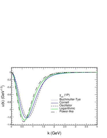
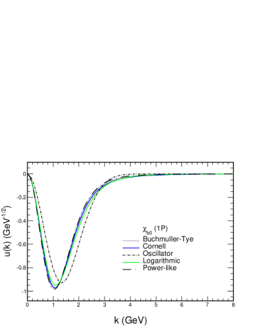
Figure 1: Quarkonium wave functions $u(k)$ for the $\chi_{c0}$ and the $\chi_{b0}$ for five potentials.

The corresponding light-cone wave function is shown for example in Fig.2 for the Buchmüller-Tye potential. Similar light-front wave functions were obtained from four other potentials from the literature. The wave functions are used then to calculate $\gamma^{*}\gamma^{*}\to\chi_{c0}$ and $\gamma^{*}\gamma^{*}\to\chi_{b0}$ form factors as discussed in the previous section. For both mesons the light-cone wave function has a similar shape but in the case of the $\chi_{b0}$ the range of $k_{T}$ is broader.

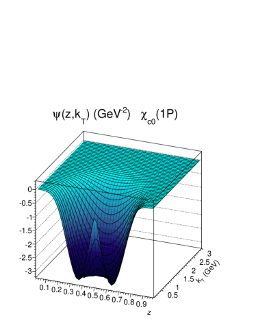
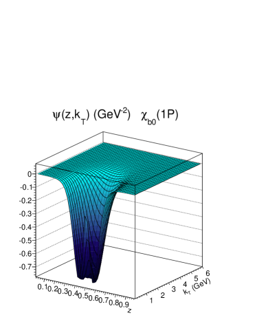
Figure 2: Light cone wave function $\psi(z,k_{T})$ for the Buchmüller-Tye potential for $\chi_{c0}$ and $\chi_{b0}$.

Some basic information on $\chi_{c0}$ and $\chi_{b0}$ mesons is collected in Tab. 1.

Table 1: Values for meson mass, $\Gamma_{tot}$, and the branching ratio ${\rm Br}(\chi_{Q0}\to\gamma\gamma)=\Gamma(\chi_{Q0}\to\gamma\gamma)/\Gamma_{tot}$ according to the Particle Data Group PDG .

	$M_{\chi}(1P)[MeV]$	$\Gamma_{tot}[MeV]$	${\rm Br}(\chi_{Q0}\to\gamma\gamma)$
$\chi_{c0}(1P)$	$3414.71\pm 0.30$	$10.8\pm 0.6$	$(2.04\pm 0.09)\cdot 10^{-4}$
$\chi_{b0}(1P)$	9859.44$\pm$0.42$\pm$0.31	-	-

The value of $|F_{TT}(0,0)|$ and decay widths at the leading and next-to-leading order obtained from different potential models are collected in Tab. 2 for $\chi_{c0}$ meson. We used the NLO expression for the radiative decay width (see Ref. Ebert:2003mu ), inserting the LO relation between $\gamma\gamma$ decay width and $F(0,0)$ from Eq. (33):

$$\Gamma(\chi_{Q0}\to\gamma\gamma)_{NLO} = \Gamma(\chi_{Q0}\to\gamma\gamma)_{LO}\Big{[}1+\frac{\alpha_{s}}{\pi}\Big{(}\frac{\pi^{2}}{3}-\frac{28}{9}\Big{)}\Big{]}\;,$$ (55)

here we employed $\alpha_{s}=0.26$ for $\chi_{c0}$ and $\alpha_{s}=0.18$ for $\chi_{b0}$ (see Ref. Ebert:2003mu ).

Using Eq. (55) and the experimental value for the radiative decay width we extracted $F_{TT}(0,0)$ for both on-shell photons at leading order.

Table 2: $F_{TT}(0,0)$ and $\Gamma(\chi\rightarrow\gamma\gamma)$ for $\chi_{c0}$ for five different potentials. The value marked by * is obtained from Eq. (33), (55).

Potential type	$|F(0,0)|[GeV]$	$\Gamma(\chi\rightarrow\gamma\gamma)_{LO}[keV]$	$\Gamma(\chi\rightarrow\gamma\gamma)_{NLO}[keV]$
Harmonic oscillator	0.18	1.56	1.58
Logarithmic	0.14	0.91	0.93
Powerlike	0.16	1.32	1.34
Cornell	0.10	0.44	0.46
Buchmülller-Tye	0.14	0.96	0.98
extracted from experiment PDG	0.21*		$2.20\pm 0.16$

Similarly $|F_{TT}(0,0)|$, but with the PDG value of $m_{c}$ PDG in the form factor is presented in Tab. 3. It is worth to notice, that the form factor is very sensitive to the quark mass. This feature of the form factor is manifested in Tabs. 2, 3 and Fig. 6.

Table 3: $F_{TT}(0,0)$ with $m_{c}=1.27\,\rm{GeV}$ and corresponding radiative widths.

Potential type	$|F_{TT}(0,0)|[GeV]$	$\Gamma(\chi_{c0}\rightarrow\gamma\gamma)_{LO}[keV]$	$\Gamma(\chi_{c0}\rightarrow\gamma\gamma)_{NLO}[keV]$
Harmonic oscillator	0.21	2.06	2.09
Logarithmic	0.18	1.54	1.56
Power-law	0.18	1.54	1.56
Cornell	0.17	1.41	1.43
Buchmülller-Tye	0.18	1.54	1.56
extracted from experiment PDG	0.21*		$2.20\pm 0.16$

We apply the same formalism also to the $\chi_{b0}$ meson. The corresponding results are summed up in Tabs. 4 and 5, respectively for the potential model $m_{b}$ value and for the PDG $m_{b}$ value.

Table 4: $|F_{TT}(0,0)|$ for $\chi_{b0}$ with quark/antiquark mass corresponding to each potential. Here $\alpha_{s}=0.18$ according to Ref. Ebert:2003mu .

Potential type	$m_{b}[GeV]$	$|F_{TT}(0,0)|[GeV]$	$\Gamma(\chi_{b0}\rightarrow\gamma\gamma)_{LO}[keV]$	$\Gamma(\chi_{b0}\rightarrow\gamma\gamma)_{NLO}[keV]$
Harmonic oscillator	4.2	0.053	0.047	0.048
Logarithmic	5.0	0.032	0.017	0.017
Power-law	4.721	0.033	0.018	0.019
Cornell	5.17	0.028	0.014	0.014
Buchmülller-Tye	4.87	0.031	0.017	0.017

Table 5: $|F_{TT}(0,0)|$ for $\chi_{b0}$ with quark/antiquark $m_{b}$ = 4.18 GeV according to PDG PDG .

Potential type	$|F_{TT}(0,0)|[GeV]$	$\Gamma(\chi_{b0}\rightarrow\gamma\gamma)_{LO}[keV]$	$\Gamma(\chi_{b0}\rightarrow\gamma\gamma)_{NLO}[keV]$
Harmonic oscillator	0.053	0.048	0.049
Logarithmic	0.045	0.034	0.035
Power-law	0.042	0.030	0.030
Cornell	0.043	0.031	0.031
Buchmülller-Tye	0.042	0.030	0.030

From Eqs. (33), (50) and (55), using the radiative decay width for $\chi_{c0}$, we extracted the first derivative of radial wave function at the origin $R^{\prime}(0)$, which is contained in Tab. 6 and compared to result obtained from Eq. (26). In Tab. 7 we listed $R^{\prime}(0)$ values for $\chi_{b0}$.

In the NR limit there is an ambiguity whether calculate the decay width using the quark mass $m_{Q}$ or the meson mass $M_{\chi}$, as to the NR acurracy $M_{\chi}=2m_{Q}$, i.e.:

$$\centering\Gamma(\chi_{Q0}\to\gamma\gamma)\@add@centering = \frac{9\cdot 2^{4}\alpha_{\rm em}^{2}e_{Q}^{4}N_{c}}{M^{4}_{\chi}}|R^{\prime}(0)|^{2}\;,\,\rm{or}\,$$ (56a)

$$\Gamma(\chi_{Q0}\to\gamma\gamma) = \frac{9\alpha_{\rm em}^{2}e_{Q}^{4}N_{c}}{m^{4}_{Q}}|R^{\prime}(0)|^{2}\;.$$ (56b)

We calculated $\Gamma(\chi_{Q0}\rightarrow\gamma\gamma)_{NLO}$ respectively for $\chi_{c0}$ and $\chi_{b0}$ (see Tab. 6 and Tab. 7) for five different potentials from the literature using first Eq. (56a) (with meson mass as in Tab. 1) and then Eq. (56b) for comparison.

Table 6: $\Gamma(\chi_{c0}\rightarrow\gamma\gamma)_{NLO}$ according to Eqs. (55), (56) with respect of quark mass for distinguished potential. $R^{\prime}(0)$ is obtained from Eq. (26) and compared to $R^{\prime}(0)$ extracted from experiment as explained in the text.

Potential type	$m_{c}$ [GeV]	R’(0) [GeV5/2]	$\Gamma(\chi_{c0}\rightarrow\gamma\gamma)_{NLO}$ [keV]	$\Gamma(\chi_{c0}\rightarrow\gamma\gamma)_{NLO}$[keV]
			Eq. (56a)	Eq. (56b)
Harmonic oscillator	1.4	0.27	2.42	5.54
Logarithmic	1.5	0.24	1.85	3.11
Powerlike	1.334	0.22	1.62	4.34
Cornell	1.84	0.32	2.51	3.38
Buchmüller-Tye	1.48	0.25	2.15	3.81
extracted from experiment PDG		$0.25\pm 0.01$	$2.20\pm 0.16$

Table 7: $\Gamma(\chi_{b0}\rightarrow\gamma\gamma)_{NLO}$ according to Eqs. (55), (56) with respect of quark mass for distinguished potential. $R^{\prime}(0)$ is obtained from Eq. (26) and compared to $R^{\prime}(0)$ extracted from experiment as explained in the text.

Potential type	$m_{b}$ [GeV]	R’(0) [GeV5/2]	$\Gamma(\chi_{b0}\rightarrow\gamma\gamma)_{NLO}[keV]$	$\Gamma(\chi_{b0}\rightarrow\gamma\gamma)_{NLO}[keV]$
			Eq. (56a)	Eq. (56b)
Harmonic oscillator	4.2	1.07	0.035	0.066
Logarithmic	5.0	1.22	0.045	0.043
Powerlike	4.721	0.98	0.029	0.035
Cornell	5.17	1.37	0.057	0.047
Buchmüller-Tye	4.87	1.13	0.038	0.041

VI The $\gamma^{*}\gamma^{*}\to\chi_{c0}$ and $\gamma^{*}\gamma^{*}\to\chi_{b0}$ form factors: numerical results

Let us now focus for a while on the form factors calculated with the help of the light-cone wave functions (see Eqs. (18), (LABEL:eq:FTT_FLL)).

The form factors $F_{TT}$ and $F_{LL}$, which have a more straightforward interpretation than $G_{1},G_{2}$, are shown in Fig. 3 for $\chi_{c0}$ and Fig. 4 for $\chi_{b0}$. There is a smooth dependence on virtualities with maxima at $Q_{1}^{2}=0$ and $Q_{2}^{2}=0$ for both mesons. One can see the required Bose symmetry under exchange of $Q_{1}^{2}$ and $Q_{2}^{2}$. The two form factors have a quite different dependence on photon virtualities. This is demonstrated in the right panel of Fig. 3 where the $F_{LL}$-to-$F_{TT}$ ratio is shown. We note, that $F_{LL}\to 0$ when either $Q_{1}^{2}\to 0$ or $Q_{2}^{2}\to 0$.

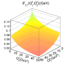
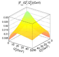
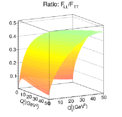
Figure 3: $|F_{TT}|$ (left) and $F_{LL}$ (middle) form factors and their ratio (right) for the Buchmüller-Tye potential for $\chi_{c0}$.

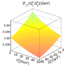
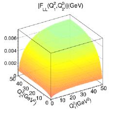
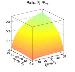
Figure 4: $|F_{TT}|$ (left) and $F_{LL}$ (right) form factors for the Buchmüller-Tye potential for $\chi_{b0}$.

In order to compare to the situation for $\gamma^{*}\gamma^{*}\to\eta_{c}(1S,2S)$ discussed in Ref. BGPSS2019 , in Fig. 5 we show the two form factors as a function of

$$\overline{Q}^{2}={Q_{1}^{2}+Q_{2}^{2}\over 2}\,\,{\rm{and}}\,\,\omega=\frac{Q_{1}^{2}-Q_{2}^{2}}{Q_{1}^{2}+Q_{2}^{2}}\,.$$ (57)

In contrast to the case of $\eta_{c}$ production BGPSS2019 we do not observe the scaling in $\omega$, neither for $F_{TT}$, nor $F_{LL}$.

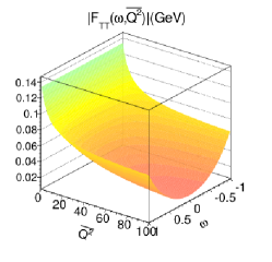
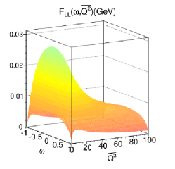
Figure 5: $|F_{TT}|$ (left) and $F_{LL}$ (right) form factors for the Buchmüller-Tye potential as a function of $\omega$ and $\bar{Q^{2}}$ for $\chi_{c0}$.

In the left panel of Fig. 6 we compare the normalized form factors $F_{TT}(Q^{2},0)/F_{TT}(0,0)$ for $\eta_{c}(1S)$ with its counterpart for $\chi_{c0}(1P)$ and $\chi_{b0}(1P)$ in the virtuality interval $Q^{2}\in$ (0,50 GeV²). For the form factor of the $\chi_{c0}$ we used the mass of the $c$-quark $m_{c}=1.27$ GeV, and for the $\chi_{b0}$ form factor, $m_{b}=4.18$ GeV. Results for five different potential models are presented for $\chi_{c0}(1P)$ and $\chi_{b0}(1P)$, whereas for the case of $\eta_{c}$(1S), we show the result from Ref. BGPSS2019 for the power-law potential model only. In the right panel we present the normalized form factors for five different potential models for $\chi_{c0}$ and $\chi_{b0}$, but with corresponding quark masses specific to each potential model.

A first measurement in $e^{+}e^{-}$ collisions of $\chi_{c0}$ production and single-tag $Q^{2}$ dependence of the cross section was done recently by the Belle collaboration Masuda:2017rhm in the $K_{S}K_{S}$ final state. The statistics is, however, too low (about 10 events) to allow detailed studies.

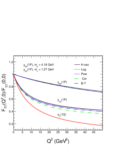
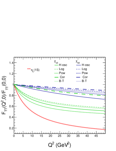
Figure 6: Normalized to unity TT form factor for three different mesons: $\eta_{c}$(1S), $\chi_{c0}$(1P), $\chi_{b0}$(1P).

VII Differential cross sections for the $pp\to\chi_{c0}$ and $pp\to\chi_{b0}$ reactions

In this subsection we shall present differential distributions in the $\chi_{c0}$ transverse momentum and rapidity for the $pp\to\chi_{c0}$ reaction as well as distributions in the same observables for $pp\to\chi_{b0}$. Here we shall set $\sqrt{s}$ = 13 TeV. The grids for $G_{1}$ and $G_{2}$ form factors are used in an interpolation procedure to obtain values relevant for the cross section calculations.

In Fig.7 we show transverse momentum distributions of $\chi_{c0}$ and $\chi_{b0}$ for the broad range of its rapidity $-6<y<6$ for different $c{\bar{c}}$ and $b{\bar{b}}$ potentials specified in the figure. There is a rather small dependence on the potential used, except for the region of $p_{T}\lesssim 5\,\rm{GeV}$. In the first row one can find the plots where we used in the form factor the quark mass corresponding to the respective $q{\bar{q}}$ potential model. The second row presents the plots with $m_{c}=1.27\,\rm{GeV}$ and $m_{b}=4.18$ GeV. In this case, in the region of meson $p_{T}<$ 5 GeV there is no strong dependence on the $q{\bar{q}}$ potential model, but in the region of $p_{T}>5\,\rm{GeV}$ for the $\chi_{c0}$ one can observe a spread of the curves.

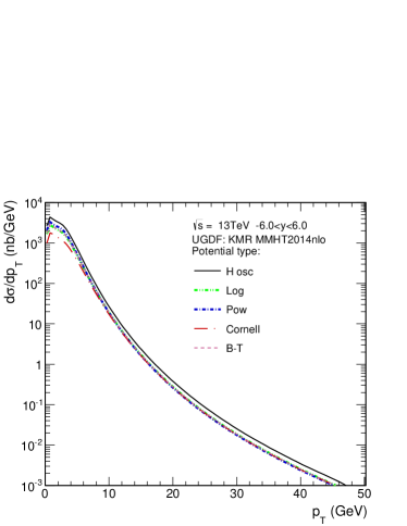
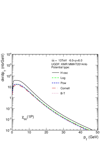
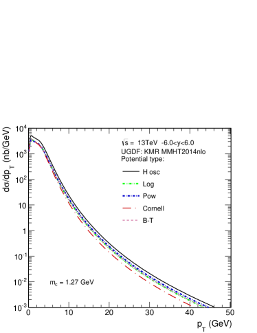
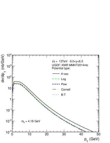
Figure 7: Comparison of $p_{T}$ distributions for five different potentials types with corresponding quark mass in the first row, and the second row is with identical (for all potentials) $m_{c}=1.27$ GeV and $m_{b}=4.18$ GeV used in calculating form factors. Here the KMR UGDF was used for $\chi_{c0}$(1P) (left panel) and $\chi_{b0}$(1P) (right panel).

In Fig.8 we compare results obtained with two different UGDs. The UGDs, which we labeled in figures as ”KMR” are based on the prescription Kimber:2001sc with updates Martin:2009ii . The KMR prescription requires as an input a collinear gluon distribution. For this purpose, we used the NLO collinear gluon distribution from Harland-Lang:2014zoa . We also employed the UGD ”JH-2013-set2” constructed from HERA data on deep inelastic structure functions as a solution of the CCFM evolution equation CCFM , which has been obtained by Hautmann and Jung Hautmann:2013tba . The corresponding results differ at small transverse momenta $p_{T}$, in the peak region of the distribution. A similar behaviour was observed recently for the production of $\eta_{c}$ in BPSS2019 .

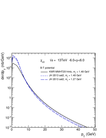
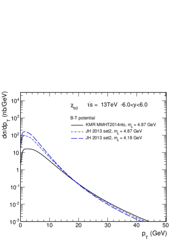
Figure 8: Comparison of $p_{T}$ distributions of $\chi_{c0}$ (left) and $\chi_{b0}$ (right) for two different UGDFs. Here the Buchmüller-Tye potential was used.

In the present analysis we explicitly calculated the $\gamma^{*}\gamma^{*}\to\chi_{c0}$ as well as $\gamma^{*}\gamma^{*}\to\chi_{b0}$ form factors as presented in the previous section. Here we wish to compare our results of corresponding cross sections with the result obtained previously Kniehl:2006sk within the NRQCD approximation. In Fig. 9 and Fig. 10 we compare our full result obtained with the Buchmüller-Tye potential with that of the NRQCD approach. Both results were obtained with the KMR UGDF.

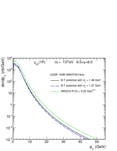
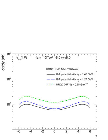
Figure 9: Comparison of $p_{T}$ distributions of $\chi_{c0}$ for our full model (solid line - with $m_{c}=1.48$ GeV, dashed line - with $m_{c}=1.27$ GeV) with the NRQCD result (see Eq.(29)) (dash-dotted line). Here the B-T potential and the KMR UGDF were used. In the NRQCD matrix element we applied $R^{\prime}(0)=0.25\,{\rm GeV}^{5/2}$ (the extracted value from the experimental radiative decay width, see Tab. 6).

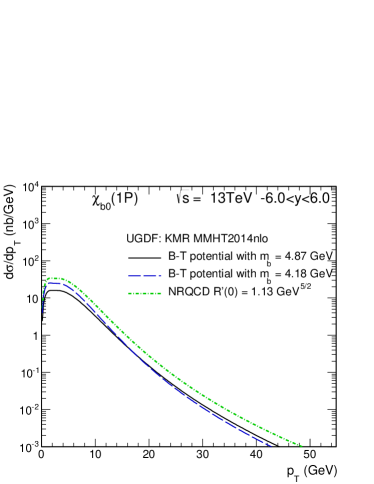
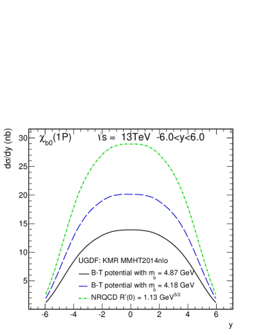
Figure 10: Comparison of $p_{T}$ distributions for our full model (solid line - with $m_{b}=4.87$ GeV, dashed line - with $m_{b}=4.18$ GeV) with the NRQCD result (see Eq.(29)) (dash-dotted line). Here the BT potential and the KMR UGDF are used.

In Fig.11 we compare our results for $\chi_{c0}$ and $\chi_{b0}$ production with that for $\eta_{c}(1S)$ production from our recent analysis BPSS2019 . The cross section for $\chi_{c0}$ production is almost an order of magnitude smaller than that for $\eta_{c}(1S)$ production. While the distributions in rapidity have a similar shape, the distributions in transverse momentum are somewhat different. The different shape of transverse momentum distribution is a reflection of different matrix elements in both cases.

Since in addition, for the branching ratios to the $p\bar{p}$ channel, we have $Br(\chi_{c0}\to p{\bar{p}})<Br(\eta_{c}\to p{\bar{p}}$), it may be very difficult to observe the $\chi_{c0}$ quarkonium in the proton-antiproton final state. Here the $\gamma\gamma$ final state could be a better option. The feasibility of such a measurement requires further Monte Carlo studies which go beyond the scope of the present paper.

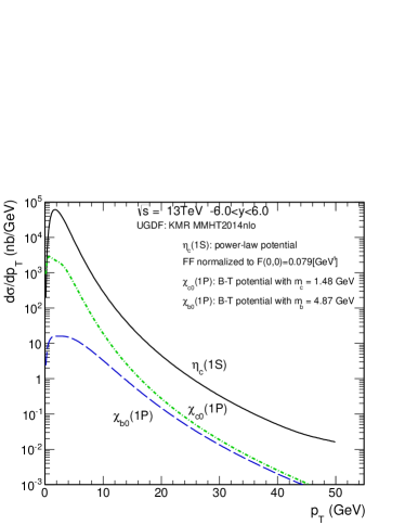
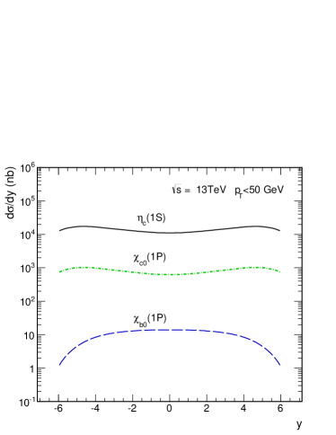
Figure 11: Differential cross section in terms of transverse momentum (lhs) and rapidity (rhs) of the meson ($\eta_{c}$, $\chi_{c0}$, $\chi_{b0}$).

Figs. 12, 13 are devoted to specific experiments: ATLAS and LHCb. On the l.h.s. we show the $q_{1T}$ or $q_{2T}$ distributions. For the ATLAS experiment they are the same, but differ for the LHCb experiment (compare the red dashed and red dotted lines). On the rhs we show the $\chi_{c0}$ transverse momentum distributions for the two experiments. A broader distribution is obtained for the ATLAS kinematics. The results presented on the rhs could be directly confronted with experimental data provided such a measurement is feasible.

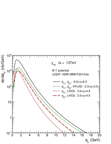
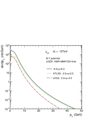
Figure 12: On the lhs differential cross section as a function of the transverse momentum of initial gluon ($q_{1T}$ or $q_{2T}$) with rapidity cuts for the ATLAS and LHCb experiments. On the rhs differential cross section as a function of the transverse momentum of $\chi_{c}$ with rapidity cuts for the ATLAS and LHCb experiments.

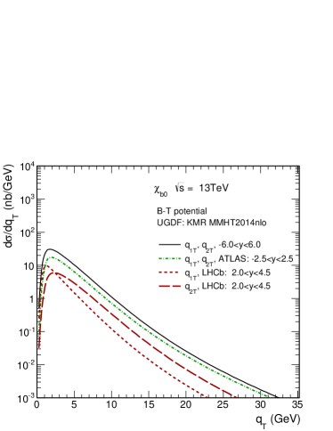
Figure 13: Differential cross section as a function of the transverse momentum of initial gluon ($q_{1T}$ or $q_{2T}$) with rapidty cuts for the ATLAS and LHCb experiments. On the rhs differential cross section as a function of the transverse momentum of $\chi_{b}$ with rapidity cuts for the ATLAS and LHCb experiments.

Let us now come to the discussion of some of the most striking results of our work, related to the polarizations of gluons. Indeed, Eq.(51) to Eq.(54) clearly show the nontrivial helicity structure of the (reggeized) gluon-gluon fusion process. Differently from the collinear approach, gluons do not only carry transverse polarizations, but also longitudinal gluons enter. The $\chi$-production cross section rather encodes the properties of a whole density matrix in the space of gluon polarizations.

In Fig. 14 and Fig. 15 we compare contributions from TT and LL amplitudes of the process $pp\to\chi_{c0}$ and $pp\to\chi_{b0}$ to their coherent sum. The LL component when separate is an order of magnitude smaller than the TT one. However, one can observe net negative interference effect – the cross section when including the LL component is smaller than that obtained for the TT component only. This is clearly visible for rapidity distributions for $\chi_{c0}$. The details depend, however, on the meson transverse momentum. The interference effect changes sign at small $p_{T}$.

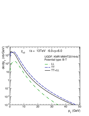
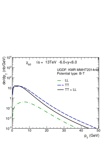
Figure 14: The comparison of meson transverse momentum distribution with only the $LL$ amplitude and only $TT$ amplitude as well as for the full, coherent sum of $TT$ and $LL$ amplitudes. Here the B-T potential was used.

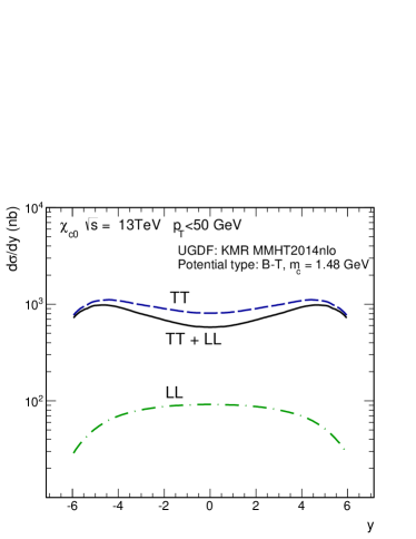
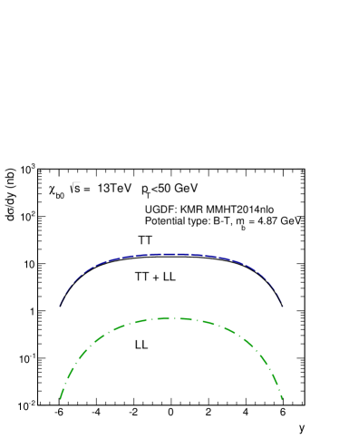
Figure 15: The comparison of meson rapidity distribution with only $LL$ amplitude and only $TT$ amplitude as well as for the full coherent sum of $TT$ and $LL$ amplitudes. Here the B-T potential was used.

VIII Conclusions

We have presented a formalism how to include $c\bar{c}$ wave functions for calculating production of $\chi_{c0}$ and $\chi_{b0}$ P-wave quarkonia in proton-proton collisions within the $k_{T}$-factorization approach. The corresponding radiative decay widths were discussed in detail. We have presented a discussion about the relevant quark mass dependence of the form factors at $Q_{1}^{2}=0$ and $Q_{2}^{2}=0$ and radiative decay widths. We have presented several tables demonstrating dependences on approximations used.

Different representations of the $\gamma^{*}\gamma^{*}\to\chi_{Q0}$ form factors were considered. We have presented and discussed the form factors as functions of ($Q_{1}^{2},Q_{2}^{2}$) and ($\bar{Q^{2}},\omega$), where $\bar{Q^{2}}=\frac{Q_{1}^{2}+Q_{2}^{2}}{2}$ and $\omega=\frac{Q_{1}^{2}-Q_{2}^{2}}{Q_{1}^{2}+Q_{2}^{2}}$. In contrast to the $\eta_{c}$ case we observe no scaling of the $F_{TT}$ and $F_{LL}$ form factors in $\omega$ for $\chi_{c0}$. We have presented also the form factors as functions of single photon virtuality. Such form factors could be measured in future by Belle2 experiments.

Similar from factors were calculated next for $g^{*}g^{*}\to\chi_{c0}$. The form factors have then been used to calculate rapidity and transverse momentum distributions of $\chi_{c0}$ at $\sqrt{s}$ = 13 TeV within the $k_{T}$-factorization approach. Two different UGDFs from the literature have been used.

We have compared the results of our full calculations with the form factors obtained with the light-cone $c\bar{c}$ wave function to the results of the NRQCD calculations as well as with those for $\eta_{c}(1S)$ production obtained recently BPSS2019 . The cross section for $\chi_{c0}$ production is somewhat smaller than that for the $\eta_{c}(1S)$ production which makes a measurement in the $p\bar{p}$ channel rather difficult. The $\gamma\gamma$ or $\gamma J/\psi$ final states might be a better option.

Finally we have performed a decomposition of the cross sections for $pp\to\chi_{c0}$ and $pp\to\chi_{b0}$ into TT, LL and their interference components. On average we have found a negative interference effect. For $\chi_{c0}$ production the inclusion of the LL components lowers the rapidity distributions - the result of the complete calculation is lower than that for the TT component alone. The interference effect depends, however, on $\chi_{c0}$ or $\chi_{b0}$ transverse momenta.

Acknowledgements

This work was partially supported by the Polish National Science Center grant UMO-2018/31/B/ST2/03537 and by the Center for Innovation and Transfer of Natural Sciences and Engineering Knowledge in Rzeszów. This work was supported by Polish National Agency for Academic Exchange under Contract No. PPN/IWA/2018/1/00031/U/0001. R.P. is partially supported by the Swedish Research Council grant No. 2016-05996, by the European Research Council (ERC) under the European Union’s Horizon 2020 research and innovation programme (grant agreement No 668679), as well as by the Ministry of Education, Youth and Sports of the Czech Republic project LTT17018 and by the NKFI grant K133046 (Hungary). Part of this work has been performed in the framework of COST Action CA15213 “Theory of hot matter and relativistic heavy-ion collisions” (THOR).

Appendix A Light-cone wave function for the scalar meson ${}^{2S+1}L_{J}=^{3}P_{0},\,J^{PC}=0^{++}$

To construct the light-front wave function of the $Q\bar{Q}$ bound state of good angular momentum quantum numbers we use the procedure based on the Melosh tranformation Melosh:1974cu ; Jaus:1989au and Terentev substitution Terentev:1976jk starting from the quark-model rest-frame wave function (WF). For the scalar meson, which is a $J=0$, $L=1,S=1$ state, the rest-frame WF has the form

$$\Psi_{\tau\bar{\tau}}(\vec{k}) = \sum_{L_{z},S_{z}}Y_{1L_{z}}(\hat{k})\langle{{1\over 2}{1\over 2}\tau\bar{\tau}}|{1S_{z}}\rangle\langle{11L_{z}S_{z}}|{00}\rangle{u(k)\over k}$$ (58)

$$= {1\over\sqrt{2}}\xi^{\tau\dagger}_{Q}\,{(\vec{\sigma}\cdot\vec{k})\over k}i\sigma_{2}\,\xi^{\bar{\tau}*}_{\bar{Q}}\,{u(k)\over k}{1\over\sqrt{4\pi}}.$$

Here, following the notation of Cepila:2019skb , $\xi_{Q}^{\tau},\xi_{\bar{Q}}^{\bar{\tau}*}$ are the canonical two-spinors of quark and antiquark respectively. The wave function is normalized as

$$\int d^{3}\vec{k}\,\sum_{\tau\bar{\tau}}|\Psi_{\tau\bar{\tau}}(\vec{k})|^{2}=1,$$ (59)

which implies for the radial WF $u_{1}(k)$, that

$$\int_{0}^{\infty}dk\,u^{2}(k)=1.$$ (60)

We now wish to express the spin-orbit structure in terms of light front spinors $\chi_{Q}^{\lambda},\chi_{\bar{Q}}^{\bar{\lambda}*}$, which are related to the canonical spinors via the Melosh-transform:

$$\xi_{Q} = R(z,\mbox{\boldmath$k$})\chi_{Q}$$

$$\xi^{*}_{\bar{Q}} = R^{*}(1-z,-\mbox{\boldmath$k$})\chi^{*}_{\bar{Q}}\,,$$ (61)

with the unitary matrix $R(z,\mbox{\boldmath$k$})$

$$R(z,\mbox{\boldmath$k$})={m_{Q}+zM-i\vec{\sigma}\cdot(\vec{n}\times\mbox{\boldmath$k$})\over\sqrt{(m_{Q}+zM)^{2}+\mbox{\boldmath$k$}^{2}}}={m_{Q}+zM-i\vec{\sigma}\cdot(\vec{n}\times\mbox{\boldmath$k$})\over\sqrt{zM(M+2m_{Q})}}\,.$$ (62)

Here $z$ and $1-z$ are the fractions of the meson’s lightfront plus-momentum carried by the quark and antiquark respectively, while their transverse momenta are denoted by $\pm\mbox{\boldmath$k$}$. We also introduced $\vec{n}=(0,0,1)$ and the vector product $\vec{n}\times\mbox{\boldmath$k$}=(-k_{y},k_{x},0)$. The three-momentum $\vec{k}$ in the $Q\bar{Q}$ rest frame is parametrized as

$$\vec{k}=(\mbox{\boldmath$k$},k_{z})=(\mbox{\boldmath$k$},{1\over 2}(2z-1)M)\,,$$ (63)

where $M$ is the invariant mass of the $Q\bar{Q}$ system obtained from

$$M^{2}={\mbox{\boldmath$k$}^{2}+m_{Q}^{2}\over z(1-z)}.$$ (64)

Notice also, that

$$k=|\vec{k}|={1\over 2}\sqrt{M^{2}-4m_{Q}^{2}}\,.$$ (65)

The light-front wave function depending on light-front helicities $\lambda\bar{\lambda}$ now has the form

$$\Psi_{\lambda\bar{\lambda}}(z,\mbox{\boldmath$k$})=\chi_{Q}^{\lambda\dagger}\,{\cal O}^{\prime}\,i\sigma_{2}\,\chi_{\bar{Q}}^{\bar{\lambda}*}\,\phi(z,\mbox{\boldmath$k$})\;.$$ (66)

Here the radial light-front wave function is expressed as

$$\phi(z,\mbox{\boldmath$k$})={u(k)\over k}\,{\sqrt{{\cal J}}\over\sqrt{4\pi}}\;,$$ (67)

where ${\cal J}$ is a jacobian for the transition from integration over $\vec{k}$ to the relativistic two-body phase space parametrized through $z,\mbox{\boldmath$k$}$:

$$d^{3}\vec{p}={\cal J}{dzd^{2}\mbox{\boldmath$k$}\over z(1-z)16\pi^{3}}\,,$$ (68)

which gives $\sqrt{{\cal J}}=2\sqrt{M\pi^{3}}$, so that

$$\phi(z,\mbox{\boldmath$k$})=\pi\sqrt{M}{u(k)\over k}.$$ (69)

Let us turn now to the spin-orbit factor. Denoting ${\cal O}=\vec{\sigma}\cdot\vec{k}/(\sqrt{2}k)$, we can write the Melosh-transformed spin-orbit vertex as

$${\cal O}^{\prime}=R^{\dagger}(z,\mbox{\boldmath$k$}){\cal O}\,i\sigma_{2}R^{*}(1-z,-\mbox{\boldmath$k$})(i\sigma_{2})^{-1}=R^{\dagger}(z,\mbox{\boldmath$k$}){\cal O}\,R(1-z,-\mbox{\boldmath$k$})\,.$$ (70)

In the last equality, we used the property of Pauli-matrices

$$i\sigma_{2}\,\vec{\sigma}^{*}\,(i\sigma_{2})^{-1}=-\vec{\sigma}\,.$$ (71)

Inserting the explicit form of matrices $R$, we obtain

$${\cal O}^{\prime} = {1\over\sqrt{z(1-z)}}{1\over M(M+2m_{Q})}\Big{\{}(m_{Q}^{2}+m_{Q}M+z(1-z)M^{2}){\cal O}$$ (72)

$$-\vec{\sigma}\cdot(\vec{n}\times\mbox{\boldmath$k$})\,{\cal O}\,\vec{\sigma}\cdot(\vec{n}\times\mbox{\boldmath$k$})$$

$$+(M+2m_{Q}){i\over 2}\Big{(}{\cal O}\,\vec{\sigma}\cdot(\vec{n}\times\mbox{\boldmath$k$})+\vec{\sigma}\cdot(\vec{n}\times\mbox{\boldmath$k$})\,{\cal O}\Big{)}$$

$$+(2z-1)M{i\over 2}\Big{(}{\cal O}\,\vec{\sigma}\cdot(\vec{n}\times\mbox{\boldmath$k$})-\vec{\sigma}\cdot(\vec{n}\times\mbox{\boldmath$k$})\,{\cal O}\Big{)}\Big{\}}.$$

For the case of interest, using the well known properties of Pauli matrices, we arrive at

$${\cal O}^{\prime}={1\over\sqrt{z(1-z)}}{1\over 2\sqrt{2}k}\Big{\{}\vec{\sigma}\cdot\mbox{\boldmath$k$}+(2z-1)m_{Q}\,\vec{\sigma}\cdot\vec{n}\Big{\}}\,.$$ (73)

We note in passing, that the effect of the Melosh rotation is simply a substitution of

$$\vec{k}\to\vec{k}^{\prime}=\Big{(}{\mbox{\boldmath$k$}\over 2\sqrt{z(1-z)}},{(2z-1)m_{Q}\over 2\sqrt{z(1-z)}}\Big{)}\,,$$ (74)

in the spin-orbit part of Eq.(58).

Inserting this into Eq.(66) gives us the following components of the light-front wave function:

$$\Psi_{\lambda\bar{\lambda}}(z,\mbox{\boldmath$k$}) = \begin{pmatrix}\Psi_{++}(z,\mbox{\boldmath$k$})&\Psi_{+-}(z,\mbox{\boldmath$k$})\\ \Psi_{-+}(z,\mbox{\boldmath$k$})&\Psi_{--}(z,\mbox{\boldmath$k$})\end{pmatrix}$$ (75)

$$= {-1\over\sqrt{z(1-z)}}\begin{pmatrix}k_{x}-ik_{y}&m_{Q}(1-2z)\\ m_{Q}(1-2z)&-k_{x}-ik_{y}\end{pmatrix}{\phi(z,\mbox{\boldmath$k$})\over\sqrt{2}\sqrt{M^{2}-4m_{Q}^{2}}}\,.$$

To lighten up the notation in the rest of the paper, we further absorb a factor $1/(2\sqrt{2}k)$ into the wave function, and introduce

$$\psi(z,\mbox{\boldmath$k$})\equiv{\phi(z,\mbox{\boldmath$k$})\over\sqrt{2}\sqrt{M^{2}-4m_{Q}^{2}}}\,.$$ (76)

The normalization condition reads

$$1 = \int{dzd^{2}\mbox{\boldmath$k$}\over z(1-z)16\pi^{3}}\sum_{\lambda,\bar{\lambda}}|\Psi_{\lambda\bar{\lambda}}(z,\mbox{\boldmath$k$})|^{2}=\int{dzd^{2}\mbox{\boldmath$k$}\over z(1-z)16\pi^{3}}\,|\phi(z,\mbox{\boldmath$k$})|^{2}$$ (77)

$$= \int{dzd^{2}\mbox{\boldmath$k$}\over z(1-z)16\pi^{3}}\,2(M^{2}-4m_{Q}^{2})\,|\psi(z,\mbox{\boldmath$k$})|^{2}\,.$$

References

• (1) J. P. Lansberg, “New Observables in Inclusive Production of Quarkonia,” arXiv:1903.09185 [hep-ph].
• (2) A. Chisholm, “Measurements of the $\chi_{c}$ and $\chi_{b}$ quarkonium states in $pp$ collisions with the ATLAS experiment”, Springer Theses (2014).
• (3) I. M. Belyaev and V. Y. Egorychev, Phys. Atom. Nucl.  78, no. 8, 977 (2015) [Yad. Fiz.  78, no. 11, 1036 (2015)].
• (4) S. P. Baranov and A. V. Lipatov, Phys. Rev. D 100, no. 11, 114021 (2019).
• (5) P. Hägler, R. Kirschner, A. Schäfer, L. Szymanowski and O. V. Teryaev, Phys. Rev. Lett.  86 1446 (2001).
• (6) B. A. Kniehl, D. V. Vasin and V. A. Saleev, Phys. Rev. D 73, 074022 (2006).
• (7) S. P. Baranov, A. V. Lipatov and N. P. Zotov, Phys. Rev. D 93, no. 9, 094012 (2016).
• (8) A. Cisek and A. Szczurek, Phys. Rev. D 97, no. 3, 034035 (2018).
• (9) A. K. Likhoded, A. V. Luchinsky and S. V. Poslavsky, Phys. Rev. D 86, 074027 (2012).
• (10) A. K. Likhoded, A. V. Luchinsky and S. V. Poslavsky, Phys. Rev. D 90, no. 7, 074021 (2014).
• (11) D. Diakonov, M. G. Ryskin and A. G. Shuvaev, JHEP 1302, 069 (2013).
• (12) D. Boer and C. Pisano, Phys. Rev. D 86, 094007 (2012).
• (13) I. Babiarz, V. P. Goncalves, R. Pasechnik, W. Schäfer and A. Szczurek, Phys. Rev. D 100, no. 5, 054018 (2019).
• (14) I. Babiarz, R. Pasechnik, W. Schäfer and A. Szczurek, JHEP 2002, 037 (2020).
• (15) L. V. Gribov, E. M. Levin and M. G. Ryskin, Phys. Rept.  100, 1 (1983); E. M. Levin, M. G. Ryskin, Y. M. Shabelski and A. G. Shuvaev, Sov. J. Nucl. Phys.  53, 657 (1991) [Yad. Fiz.  53, 1059 (1991)].
• (16) S. Catani, M. Ciafaloni and F. Hautmann, Phys. Lett. B 242, 97 (1990); S. Catani, M. Ciafaloni and F. Hautmann, Nucl. Phys. B 366, 135 (1991).
• (17) J. C. Collins and R. K. Ellis, Nucl. Phys. B 360, 3 (1991).
• (18) H. J. Melosh, Phys. Rev. D 9, 1095 (1974).
• (19) W. Jaus, Phys. Rev. D 41, 3394 (1990).
• (20) M. V. Terentev, Sov. J. Nucl. Phys.  24, 106 (1976) [Yad. Fiz.  24, 207 (1976)].
• (21) J. Cepila, J. Nemchik, M. Krelina and R. Pasechnik, Eur. Phys. J. C 79, no. 6, 495 (2019).
• (22) R. S. Pasechnik, A. Szczurek and O. V. Teryaev, Phys. Rev. D 78, 014007 (2008).
• (23) V. M. Budnev, I. F. Ginzburg, G. V. Meledin and V. G. Serbo, Phys. Rept.  15, 181 (1975).
• (24) M. Poppe, Int. J. Mod. Phys. A 1 545 (1986).
• (25) J. Hüfner, Y. P. Ivanov, B. Z. Kopeliovich and A. V. Tarasov, Phys. Rev. D 62, 094022 (2000).
• (26) D. Ebert, R. N. Faustov and V. O. Galkin, Mod. Phys. Lett. A 18, 601 (2003).
• (27) M. Tanabashi et al. [Particle Data Group], Phys. Rev. D 98, no. 3, 030001 (2018).
• (28) M. Masuda et al. [Belle Collaboration], Phys. Rev. D 97, no. 5, 052003 (2018).
• (29) M. A. Kimber, A. D. Martin and M. G. Ryskin, Phys. Rev. D 63, 114027 (2001).
• (30) A. D. Martin, M. G. Ryskin and G. Watt, Eur. Phys. J. C 66, 163 (2010). G. Watt, A. D. Martin and M. G. Ryskin, Phys. Rev. D 70, 014012 (2004) Erratum: [Phys. Rev. D 70, 079902 (2004)].
• (31) L. A. Harland-Lang, A. D. Martin, P. Motylinski and R. S. Thorne, Eur. Phys. J. C 75, no. 5, 204 (2015).
• (32) M. Ciafaloni, Nucl. Phys. B 296, 49 (1988); S. Catani, F. Fiorani and G. Marchesini, Phys. Lett. B 234, 339 (1990); S. Catani, F. Fiorani and G. Marchesini, Nucl. Phys. B 336, 18 (1990).
• (33) F. Hautmann and H. Jung, Nucl. Phys. B 883, 1 (2014). F. Hautmann, H. Jung, M. Krämer, P. J. Mulders, E. R. Nocera, T. C. Rogers and A. Signori, Eur. Phys. J. C 74, 3220 (2014). H. Jung et al., Eur. Phys. J. C 70, 1237 (2010).