Stochastic Latent Residual Video Prediction

Abstract

Designing video prediction models that account for the inherent uncertainty of the future is challenging. Most works in the literature are based on stochastic image-autoregressive recurrent networks, which raises several performance and applicability issues. An alternative is to use fully latent temporal models which untie frame synthesis and temporal dynamics. However, no such model for stochastic video prediction has been proposed in the literature yet, due to design and training difficulties. In this paper, we overcome these difficulties by introducing a novel stochastic temporal model whose dynamics are governed in a latent space by a residual update rule. This first-order scheme is motivated by discretization schemes of differential equations. It naturally models video dynamics as it allows our simpler, more interpretable, latent model to outperform prior state-of-the-art methods on challenging datasets.

1 Introduction

Being able to predict the future of a video from a few conditioning frames in a self-supervised manner has many applications in fields such as reinforcement learning (Gregor et al., 2019) or robotics (Babaeizadeh et al., 2018). More generally, it challenges the ability of a model to capture visual and dynamic representations of the world. Video prediction has received a lot of attention from the computer vision community. However, most proposed methods are deterministic, reducing their ability to capture video dynamics, which are intrinsically stochastic (Denton & Fergus, 2018).

Stochastic video prediction is a challenging task which has been tackled by recent works. Most state-of-the-art approaches are based on image-autoregressive models (Denton & Fergus, 2018; Babaeizadeh et al., 2018), built around Recurrent Neural Networks (RNNs), where each generated frame is fed back to the model to produce the next frame. However, performances of their temporal models innately depend on the capacity of their encoder and decoder, as each generated frame has to be re-encoded in a latent space. Such autoregressive processes induce a high computational cost, and strongly tie the frame synthesis and temporal models, which may hurt the performance of the generation process and limit its applicability (Gregor et al., 2019; Rubanova et al., 2019).

An alternative approach consists in separating the dynamic of the state representations from the generated frames, which are independently decoded from the latent space. In addition to removing the aforementioned link between frame synthesis and temporal dynamics, this is computationally appealing when coupled with a low-dimensional latent space. Moreover, such models can be used to shape a complete representation of the state of a system, e.g. for reinforcement learning applications (Gregor et al., 2019), and are more interpretable than autoregressive models (Rubanova et al., 2019). Yet, these State-Space Models (SSMs) are more difficult to train as they require non-trivial inference schemes (Krishnan et al., 2017) and a careful design of the dynamic model (Karl et al., 2017). This leads most successful SSMs to only be evaluated on small or artificial toy tasks.

In this work, we introduce a novel stochastic dynamic model for the task of video prediction which successfully leverages structural and computational advantages of SSMs that operate on low-dimensional latent spaces. Its dynamic component determines the temporal evolution of the system through residual updates of the latent state, conditioned on learned stochastic variables. This formulation allows us to implement an efficient training strategy and process in an interpretable manner complex high-dimensional data such as videos. This residual principle can be linked to recent advances relating residual networks and Ordinary Differential Equations (ODEs) (Chen et al., 2018). This interpretation opens new perspectives such as generating videos at different frame rates, as demonstrated in our experiments. The proposed approach outperforms current state-of-the-art models on the task of stochastic video prediction, as demonstrated by comparisons with competitive baselines on representative benchmarks.

2 Related Work

Video synthesis covers a range of different tasks, such as video-to-video translation (Wang et al., 2018), super-resolution (Caballero et al., 2017), interpolation between distant frames (Jiang et al., 2018), generation (Tulyakov et al., 2018), and video prediction, which is the focus of this paper.

Deterministic models.

Inspired by prior sequence generation models using RNNs (Graves, 2013), a number of video prediction methods (Srivastava et al., 2015; Villegas et al., 2017; van Steenkiste et al., 2018; Wichers et al., 2018; Jin et al., 2020) rely on LSTMs (Long Short-Term Memory networks, Hochreiter & Schmidhuber, 1997), or, like Ranzato et al. (2014), Jia et al. (2016) and Xu et al. (2018a), on derived networks such as ConvLSTMs (Shi et al., 2015). Indeed, computer vision approaches are usually tailored to high-dimensional video sequences and propose domain-specific techniques such as pixel-level transformations and optical flow (Shi et al., 2015; Walker et al., 2015; Finn et al., 2016; Jia et al., 2016; Walker et al., 2016; Vondrick & Torralba, 2017; Liang et al., 2017; Liu et al., 2017; Lotter et al., 2017; Lu et al., 2017a; Fan et al., 2019; Gao et al., 2019) that help to produce high-quality predictions. Such predictions are, however, deterministic, thus hurting their performance as they fail to generate sharp long-term video frames (Babaeizadeh et al., 2018; Denton & Fergus, 2018). Following Mathieu et al. (2016), some works proposed to use adversarial losses (Goodfellow et al., 2014) on the model predictions to sharpen the generated frames (Vondrick & Torralba, 2017; Liang et al., 2017; Lu et al., 2017a; Xu et al., 2018b; Wu et al., 2020). Nonetheless, adversarial losses are notoriously hard to train (Goodfellow, 2016), and lead to mode collapse, thereby preventing diversity of generations.

Stochastic and image-autoregressive models.

Some approaches rely on exact likelihood maximization, using pixel-level autoregressive generation (van den Oord et al., 2016; Kalchbrenner et al., 2017; Weissenborn et al., 2020) or normalizing flows through invertible transformations between the observation space and a latent space (Kingma & Dhariwal, 2018; Kumar et al., 2020). However, they require careful design of complex temporal generation schemes manipulating high-dimensional data, thus inducing a prohibitive temporal generation cost. More efficient continuous models rely on Variational Auto-Encoders (VAEs, Kingma & Welling, 2014; Rezende et al., 2014) for the inference of low-dimensional latent state variables. Except Xue et al. (2016) and Liu et al. (2019) who learn a one-frame-ahead VAE, they model sequence stochasticity by incorporating a random latent variable per frame into a deterministic RNN-based image-autoregressive model. Babaeizadeh et al. (2018) integrate stochastic variables into the ConvLSTM architecture of Finn et al. (2016). Concurrently with He et al. (2018), Denton & Fergus (2018) use a prior LSTM conditioned on previously generated frames in order to sample random variables that are fed to a predictor LSTM; performance of such methods were improved in follow-up works by increasing networks capacities (Castrejon et al., 2019; Villegas et al., 2019). Finally, Lee et al. (2018) combine the ConvLSTM architecture and this learned prior, adding an adversarial loss on the predicted videos to sharpen them at the cost of a diversity drop. Yet, all these methods are image-autoregressive, as they feed their predictions back into the latent space, thereby tying the frame synthesis and temporal models and increasing their computational cost. Concurrently to our work, Minderer et al. (2019) propose to use the autoregressive VRNN model (Chung et al., 2015) on learned image key-points instead of raw frames. It remains unclear to which extent this change could mitigate the aforementioned problems. We instead tackle these issues by focusing on video dynamics, and propose a model that is state-space and acts on a small latent space. This approach yields better experimental results despite weaker video-specific priors.

State-space models.

Many latent state-space models have been proposed for sequence modelization (Bayer & Osendorfer, 2014; Fraccaro et al., 2016, 2017; Krishnan et al., 2017; Karl et al., 2017; Hafner et al., 2019), usually trained by deep variational inference. These methods, which use locally linear or RNN-based dynamics, are designed for low-dimensional data, as learning such models on complex data is challenging, or focus on control or planning tasks. In contrast, our fully latent method is the first one to be successfully applied to complex high-dimensional data such as videos, thanks to a temporal model based on residual updates of its latent state. It falls within the scope of a recent trend linking differential equations with neural networks (Lu et al., 2017b; Long et al., 2018), leading to the integration of ODEs, that are seen as continuous residual networks (He et al., 2016), in neural network architectures (Chen et al., 2018). However, the latter work as well as follow-ups and related works (Rubanova et al., 2019; Yıldız et al., 2019; Le Guen & Thome, 2020) are either limited to low-dimensional data, prone to overfitting or unable to handle stochasticity within a sequence. Another line of works considers stochastic differential equations with neural networks (Ryder et al., 2018; De Brouwer et al., 2019), but are limited to continuous Brownian noise, whereas video prediction additionally requires to model punctual stochastic events.

3 Model

(a) Generative model $p$.

(b) Inference model $q$.

(c) Model and inference architecture on a test sequence. The transparent block on the left depicts the prior, and those on the right correspond to the full inference performed at training time.

Figure 1: (a), (b) Proposed generative and inference models. Diamonds and circles represent, respectively, deterministic and stochastic states. (c) Corresponding architecture with two parts: inference on conditioning frames on the left, generation for extrapolation on the right. $h_{\phi}$ and $g_{\theta}$ are deep Convolutional Neural Networks (CNNs), and other named networks are Multilayer Perceptrons (MLPs).

We consider the task of stochastic video prediction, consisting in approaching, given a number of conditioning video frames, the distribution of possible future frames.

3.1 Latent Residual Dynamic Model

Let $\bm{x}_{1\mathrel{\mathop{\ordinarycolon}}T}$ be a sequence of $T$ video frames. We model their evolution by introducing latent variables $\bm{y}$ that are driven by a dynamic temporal model. Each frame $\bm{x}_{t}$ is then generated from the corresponding latent state $\bm{y}_{t}$ only, making the dynamics independent from the previously generated frames.

We propose to model the transition function of the latent dynamic of $\bm{y}$ with a stochastic residual network. State $\bm{y}_{t+1}$ is chosen to deterministically depend on the previous state $\bm{y}_{t}$, conditionally to an auxiliary random variable $\bm{z}_{t+1}$. These auxiliary variables encapsulate the randomness of the video dynamics. They have a learned factorized Gaussian prior that depends on the previous state only. The model is depicted in Figure 1(a), and defined as follows:

$$\begin{cases}\bm{y}_{1}\sim{\mathcal{N}}(\bm{0},I),\\ \bm{z}_{t+1}\sim{\mathcal{N}}\left(\mu_{\theta}\left(\bm{y}_{t}\right),\sigma_{\theta}\left(\bm{y}_{t}\right)I\right),\\ \bm{y}_{t+1}=\bm{y}_{t}+f_{\theta}\left(\bm{y}_{t},\bm{z}_{t+1}\right),\\ \bm{x}_{t}\sim{\mathcal{G}}\left(g_{\theta}\left(\bm{y}_{t}\right)\right),\end{cases}$$ (1)

where $\mu_{\theta}$, $\sigma_{\theta}$, $f_{\theta}$ and $g_{\theta}$ are neural networks, and ${\mathcal{G}}\left(g_{\theta}\left(\bm{y}_{t}\right)\right)$ is a probability distribution parameterized by $g_{\theta}\left(\bm{y}_{t}\right)$. In our experiments, ${\mathcal{G}}$ is a normal distribution with mean $g_{\theta}\left(\bm{y}_{t}\right)$ and constant diagonal variance. Note that $\bm{y}_{1}$ is assumed to have a standard Gaussian prior, and, in our VAE setting, will be inferred from conditioning frames for the prediction task, as shown in Section 3.3.

The residual update rule takes inspiration in the Euler discretization scheme of differential equations. The state of the system $\bm{y}_{t}$ is updated by its first-order movement, i.e., the residual $f_{\theta}\left(\bm{y}_{t},\bm{z}_{t+1}\right)$. Compared to a regular RNN, this simple principle makes our temporal model lighter and more interpretable. Equation 1, however, differs from a discretized ODE because of the introduction of the stochastic discrete-time variables $\bm{z}$. Nonetheless, we propose to allow the Euler step size $\Delta t$ to be smaller than $1$, as a way to make the temporal model closer to a continuous dynamics. The updated dynamics becomes, with $\frac{1}{\Delta t}\in{\mathbb{N}}$ to synchronize the step size with the video frame rate:

$$\bm{y}_{t+\Delta t}=\bm{y}_{t}+\Delta t\cdot f_{\theta}\left(\bm{y}_{t},\bm{z}_{\lfloor t\rfloor+1}\right).$$ (2)

For this formulation, the auxiliary variable $\bm{z}_{t}$ is kept constant between two integer time steps. Note that a different $\Delta t$ can be used during training or testing. This allows our model to generate videos at an arbitrary frame rate since each intermediate latent state can be decoded in the observation space. This ability enables us to observe the quality of the learned dynamic as well as challenge its ODE inspiration by testing its generalization to the continuous limit in Section 4. In the following, we consider $\Delta t$ as a hyperparameter. For the sake of clarity, we consider that $\Delta t=1$ in the remaining of this section; generalizing to a smaller $\Delta t$ is straightforward as Figure 1(a) remains unchanged.

3.2 Content Variable

Some components of video sequences can be static, such as the background or shapes of moving objects. They may not impact the dynamics; we therefore model them separately, in the same spirit as Denton & Birodkar (2017) and Yingzhen & Mandt (2018). We compute a content variable $\bm{w}$ that remains constant throughout the whole generation process and is fed together with $\bm{y}_{t}$ into the frame generator. It enables the dynamical part of the model to focus only on movement, hence being lighter and more stable. Moreover, it allows us to leverage architectural advances in neural networks, such as skip connections (Ronneberger et al., 2015), to produce more realistic frames.

This content variable is a deterministic function $c_{\psi}$ of a fixed number $k<T$ of frames $\bm{x}_{\mathrm{c}}^{\left(k\right)}=\left(\bm{x}_{i_{1}},\ldots,\bm{x}_{i_{k}}\right)$:

$$\begin{cases}\bm{w}=c_{\psi}\left(\bm{x}_{\mathrm{c}}^{\left(k\right)}\right)=c_{\psi}\left(\bm{x}_{i_{1}},\ldots,\bm{x}_{i_{k}}\right)\\ \bm{x}_{t}\sim{\mathcal{G}}\left(g_{\theta}\left(\bm{y}_{t},\bm{w}\right)\right).\end{cases}$$ (3)

During testing, $\bm{x}_{\mathrm{c}}^{\left(k\right)}$ are the last $k$ conditioning frames (usually between $2$ and $5$).

This content variable is not endowed with any probabilistic prior, contrary to the dynamic variables $\bm{y}$ and $\bm{z}$. Thus, the information it contains is not constrained in the loss function (see Section 3.3), but only architecturally. To prevent temporal information from leaking in $\bm{w}$, we propose to uniformly sample these $k$ frames within $\bm{x}_{1\mathrel{\mathop{\ordinarycolon}}T}$ during training. We also design $c_{\psi}$ as a permutation-invariant function (Zaheer et al., 2017), consisting in an MLP fed with the sum of individual frame representations, following Santoro et al. (2017).

This absence of prior and its architectural constraint allows $\bm{w}$ to contain as much non-temporal information as possible, while preventing it from containing dynamic information. On the other hand, due to their strong standard Gaussian priors, $\bm{y}$ and $\bm{z}$ are encouraged to discard unnecessary information. Therefore, $\bm{y}$ and $\bm{z}$ should only contain temporal information that could not be captured by $\bm{w}$.

Note that this content variable can be removed from our model, yielding a more classical deep state-space model. An experiment in this setting is presented in Appendix E.

3.3 Variational Inference and Architecture

Following the generative process depicted in Figure 1(a), the conditional joint probability of the full model, given a content variable $\bm{w}$, can be written as:

$$\begin{multlined}p\left(\bm{x}_{1\mathrel{\mathop{\ordinarycolon}}T},\bm{z}_{2\mathrel{\mathop{\ordinarycolon}}T},\bm{y}_{1\mathrel{\mathop{\ordinarycolon}}T}\;\middle|\;\bm{w}\right)\\ =p\left(\bm{y}_{1}\right)\prod_{t=2}^{T}p\left(\bm{z}_{t},\bm{y}_{t}\;\middle|\;\bm{y}_{t-1}\right)\prod_{t=1}^{T}p\left(\bm{x}_{t}\;\middle|\;\bm{y}_{t},\bm{w}\right),\end{multlined}p\left(\bm{x}_{1\mathrel{\mathop{\ordinarycolon}}T},\bm{z}_{2\mathrel{\mathop{\ordinarycolon}}T},\bm{y}_{1\mathrel{\mathop{\ordinarycolon}}T}\;\middle|\;\bm{w}\right)\\ =p\left(\bm{y}_{1}\right)\prod_{t=2}^{T}p\left(\bm{z}_{t},\bm{y}_{t}\;\middle|\;\bm{y}_{t-1}\right)\prod_{t=1}^{T}p\left(\bm{x}_{t}\;\middle|\;\bm{y}_{t},\bm{w}\right),$$ (4)

with

$$p\left(\bm{z}_{t},\bm{y}_{t}\;\middle|\;\bm{y}_{t-1}\right)=p\left(\bm{z}_{t}\;\middle|\;\bm{y}_{t-1}\right)p\left(\bm{y}_{t}\;\middle|\;\bm{y}_{t-1},\bm{z}_{t}\right).$$ (5)

According to the expression of $\bm{y}_{t+1}$ in Equation 1, $p\left(\bm{y}_{t}\;\middle|\;\bm{y}_{t-1},\bm{z}_{t}\right)=\delta\left(\bm{y}_{t}-\bm{y}_{t-1}-f_{\theta}\left(\bm{y}_{t-1},\bm{z}_{t}\right)\right)$, where $\delta$ is the Dirac delta function centered on $\bm{0}$. Hence, in order to optimize the likelihood of the observed videos $p\left(\bm{x}_{1\mathrel{\mathop{\ordinarycolon}}T}\;\middle|\;\bm{w}\right)$, we need to infer latent variables $\bm{y}_{1}$ and $\bm{z}_{2\mathrel{\mathop{\ordinarycolon}}T}$. This is done by deep variational inference using the inference model parameterized by $\phi$ and shown in Figure 1(b), which comes down to considering a variational distribution $q_{Z,Y}$ defined and factorized as follows:

$$\begin{multlined}q_{Z,Y}\triangleq q\left(\bm{z}_{2\mathrel{\mathop{\ordinarycolon}}T},\bm{y}_{1\mathrel{\mathop{\ordinarycolon}}T}\;\middle|\;\bm{x}_{1\mathrel{\mathop{\ordinarycolon}}T},\bm{w}\right)\\ =q\left(\bm{y}_{1}\;\middle|\;\bm{x}_{1\mathrel{\mathop{\ordinarycolon}}k}\right)\prod_{t=2}^{T}q\left(\bm{z}_{t}\;\middle|\;\bm{x}_{1\mathrel{\mathop{\ordinarycolon}}t}\right)\underbrace{q\left(\bm{y}_{t}\;\middle|\;\bm{y}_{t-1},\bm{z}_{t}\right)}_{=p\left(\bm{y}_{t}\;\middle|\;\bm{y}_{t-1},\bm{z}_{t}\right)},\end{multlined}q_{Z,Y}\triangleq q\left(\bm{z}_{2\mathrel{\mathop{\ordinarycolon}}T},\bm{y}_{1\mathrel{\mathop{\ordinarycolon}}T}\;\middle|\;\bm{x}_{1\mathrel{\mathop{\ordinarycolon}}T},\bm{w}\right)\\ =q\left(\bm{y}_{1}\;\middle|\;\bm{x}_{1\mathrel{\mathop{\ordinarycolon}}k}\right)\prod_{t=2}^{T}q\left(\bm{z}_{t}\;\middle|\;\bm{x}_{1\mathrel{\mathop{\ordinarycolon}}t}\right)\underbrace{q\left(\bm{y}_{t}\;\middle|\;\bm{y}_{t-1},\bm{z}_{t}\right)}_{=p\left(\bm{y}_{t}\;\middle|\;\bm{y}_{t-1},\bm{z}_{t}\right)},$$ (6)

with $q\left(\bm{y}_{t}\;\middle|\;\bm{y}_{t-1},\bm{z}_{t}\right)=p\left(\bm{y}_{t}\;\middle|\;\bm{y}_{t-1},\bm{z}_{t}\right)$ being the aforementioned Dirac delta function. This yields the following evidence lower bound (ELBO), whose full derivation is given in Appendix A:

$$\log p\left(\bm{x}_{1\mathrel{\mathop{\ordinarycolon}}T}\;\middle|\;\bm{w}\right)\geq{\mathcal{L}}\left(\bm{x}_{1\mathrel{\mathop{\ordinarycolon}}T};\bm{w},\theta,\phi\right)$$ (7)

$$\triangleq -D_{\mathrm{KL}}\left(q\left(\bm{y}_{1}\;\middle|\;\bm{x}_{1\mathrel{\mathop{\ordinarycolon}}k}\right)\;\middle\|\;p\left(\bm{y}_{1}\right)\right)$$

$$+\mathbb{E}_{\left(\widetilde{\bm{z}}_{2\mathrel{\mathop{\ordinarycolon}}T},\widetilde{\bm{y}}_{1\mathrel{\mathop{\ordinarycolon}}T}\right)\sim q_{Z,Y}}\left[\sum_{t=1}^{T}\log p\left(\bm{x}_{t}\;\middle|\;\widetilde{\bm{y}}_{t},\bm{w}\right)\right.$$

$$\left.\mathop{\hphantom{+}}-\sum_{t=2}^{T}D_{\mathrm{KL}}\left(q\left(\bm{z}_{t}\;\middle|\;\bm{x}_{1\mathrel{\mathop{\ordinarycolon}}t}\right)\;\middle\|\;p\left(\bm{z}_{t}\;\middle|\;\widetilde{\bm{y}}_{t-1}\right)\right)\right],$$

where $D_{\mathrm{KL}}$ denotes the Kullback–Leibler (KL) divergence (Kullback & Leibler, 1951).

The sum of KL divergence expectations implies to consider the full past sequence of inferred states for each time step, due to the dependence on conditionally deterministic variables $\bm{y}_{2\mathrel{\mathop{\ordinarycolon}}T}$. However, optimizing ${\mathcal{L}}\left(\bm{x}_{1\mathrel{\mathop{\ordinarycolon}}T};\bm{w},\theta,\phi\right)$ with respect to model parameters $\theta$ and variational parameters $\phi$ can be done efficiently by sampling a single full sequence of states from $q_{Z,Y}$ per example, and computing gradients by backpropagation (Rumelhart et al., 1988) trough all inferred variables, using the reparameterization trick (Kingma & Welling, 2014; Rezende et al., 2014). We classically choose $q\left(\bm{y}_{1}\;\middle|\;\bm{x}_{1\mathrel{\mathop{\ordinarycolon}}k}\right)$ and $q\left(\bm{z}_{t}\;\middle|\;\bm{x}_{1\mathrel{\mathop{\ordinarycolon}}t}\right)$ to be factorized Gaussian so that all KL divergences can be computed analytically.

We include an $\ell_{2}$ regularization term on residuals $f_{\theta}$ applied to $\bm{y}$ which stabilizes the temporal dynamics of the residual network, as noted by Behrmann et al. (2019), de Bézenac et al. (2019) and Rousseau et al. (2019). Given a set of videos ${\mathcal{X}}$, the full optimization problem, where ${\mathcal{L}}$ is defined as in Equation 7, is then given as:

$$\begin{multlined}\operatorname*{arg\,max}_{\theta,\phi,\psi}\sum_{\bm{x}\in{\mathcal{X}}}\left[\mathop{\vphantom{\sum_{t=2}^{T}}}\mathbb{E}_{\bm{x}_{\mathrm{c}}^{\left(k\right)}}{\mathcal{L}}\left(\bm{x}_{1\mathrel{\mathop{\ordinarycolon}}T};c_{\psi}\left(\bm{x}_{\mathrm{c}}^{\left(k\right)}\right),\theta,\phi\right)\right.\\ \left.-\lambda\cdot\mathbb{E}_{(\bm{z}_{2\mathrel{\mathop{\ordinarycolon}}T},\bm{y}_{1\mathrel{\mathop{\ordinarycolon}}T})\sim q_{Z,Y}}\sum_{t=2}^{T}\left\|f_{\theta}\left(\bm{y}_{t-1},\bm{z}_{t}\right)\right\|_{2}\right].\end{multlined}\operatorname*{arg\,max}_{\theta,\phi,\psi}\sum_{\bm{x}\in{\mathcal{X}}}\left[\mathop{\vphantom{\sum_{t=2}^{T}}}\mathbb{E}_{\bm{x}_{\mathrm{c}}^{\left(k\right)}}{\mathcal{L}}\left(\bm{x}_{1\mathrel{\mathop{\ordinarycolon}}T};c_{\psi}\left(\bm{x}_{\mathrm{c}}^{\left(k\right)}\right),\theta,\phi\right)\right.\\ \left.-\lambda\cdot\mathbb{E}_{(\bm{z}_{2\mathrel{\mathop{\ordinarycolon}}T},\bm{y}_{1\mathrel{\mathop{\ordinarycolon}}T})\sim q_{Z,Y}}\sum_{t=2}^{T}\left\|f_{\theta}\left(\bm{y}_{t-1},\bm{z}_{t}\right)\right\|_{2}\right].$$ (8)

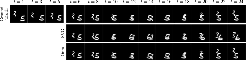
Figure 2: Conditioning frames and corresponding ground truth and best samples with respect to PSNR from SVG and our method for an example of the Stochastic Moving MNIST dataset.

Figure 1(c) depicts the full architecture of our temporal model, showing how the model is applied during testing. The first latent variables are inferred with the conditioning framed and are then predicted with the dynamic model. In contrast, during training, each frame of the input sequence is considered for inference, which is done as follows. Firstly, each frame $\bm{x}_{t}$ is independently encoded into a vector-valued representation $\widetilde{\bm{x}}_{t}$, with $\widetilde{\bm{x}}_{t}=h_{\phi}\left(\bm{x}_{t}\right)$. $\bm{y}_{1}$ is then inferred using an MLP on the first $k$ encoded frames $\widetilde{\bm{x}}_{1\mathrel{\mathop{\ordinarycolon}}k}$. Each $\bm{z}_{t}$ is inferred in a feed-forward fashion with an LSTM on the encoded frames. Inferring $\bm{z}$ this way experimentally performs better than, e.g., inferring them from the whole sequence $\bm{x}_{1\mathrel{\mathop{\ordinarycolon}}T}$; we hypothesize that this follows from the fact that this filtering scheme is closer to the prediction setting, where the future is not available.

4 Experiments

This section exposes the experimental results of our method on four standard stochastic video prediction datasets. We compare our method with state-of-the-art baselines on stochastic video prediction. Furthermore, we qualitatively study the dynamics and latent space learned by our model. Training details are described in Appendix C.

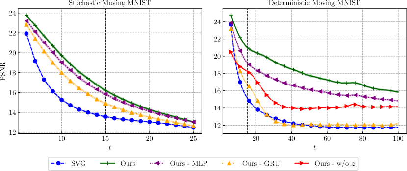
Figure 3: Mean PSNR scores with respect to $t$ for all tested models on the Moving MNIST dataset, with their $95\%$-confidence intervals. Vertical bars mark the length of training sequences.

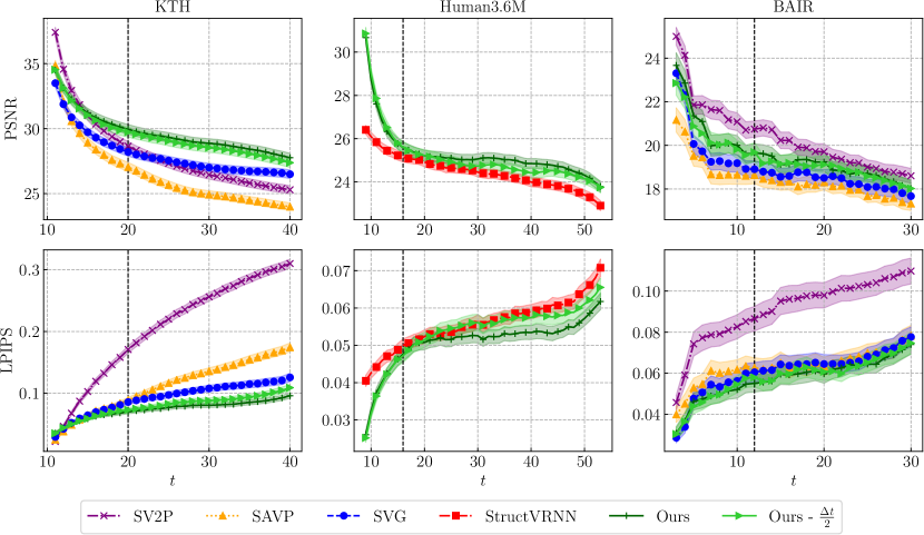
Figure 4: PSNR and LPIPS scores with respect to $t$ for all tested models on the KTH (left column), Human3.6M (center) and BAIR (right) datasets, with their $95\%$-confidence intervals. Vertical bars mark the length of training sequences.

Table 1: FVD scores for all tested methods on the KTH, Human3.6M and BAIR datasets with their $95\%$-confidence intervals over five different samples from the models. Bold scores indicate the best performing method for each dataset.

Dataset	SV2P	SAVP	SVG	StructVRNN	Ours	Ours - $\frac{\Delta t}{2}$	Ours - MLP	Ours - GRU
KTH	$636$ p m 1	$374$ p m 3	$377$ p m 6	—	$222$ p m 3	$244$ p m 3	$255$ p m 4	$240$ p m 5
Human3.6M	—	—	—	$556$ p m 9	$416$ p m 5	$415$ p m 3	$582$ p m 4	$1050$ p m 20
BAIR	$965$ p m 17	$152$ p m 9	$255$ p m 4	—	$163$ p m 4	$222$ p m 42	$162$ p m 4	$178$ p m 10

The stochastic nature and novelty of the task of stochastic video prediction make it challenging to evaluate (Lee et al., 2018): since videos and models are stochastic, comparing the ground truth and a predicted video is not adequate. We thus adopt the common approach (Denton & Fergus, 2018; Lee et al., 2018) consisting in, for each test sequence, sampling from the tested model a given number (here, $100$) of possible futures and reporting the best performing sample against the true video. We report this discrepancy for three commonly used metrics that are computed frame-wise and averaged over time: Peak Signal-to-Noise Ratio (PSNR, higher is better), Structured Similarity (SSIM, higher is better), and Learned Perceptual Image Patch Similarity (LPIPS, lower is better, Zhang et al., 2018). PSNR greatly penalizes errors in predicted dynamics, as it is a pixel-level measure derived from the $\ell_{2}$ distance, but might also favor blurry predictions. SSIM (only reported in Appendix D for the sake of concision) rather compares local frame patches to circumvent this issue, but loses some dynamics information. LPIPS compares images through a learned distance between activations of deep CNNs trained on image classification tasks, and has been shown to better correlate with human judgment on real images. Finally, the recently proposed Fréchet Video Distance (FVD, lower is better, Unterthiner et al., 2018) aims at directly comparing the distribution of predicted videos with the ground truth distribution through the representations computed by a deep CNN trained on action recognition tasks. It has been shown, independently from LPIPS, to better capture the realism of predicted videos than PSNR and SSIM. We treat all four metrics as complementary, as they capture different scales and modalities.

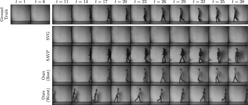
Figure 5: Conditioning frames and corresponding ground truth, best samples from SVG, SAVP and our method, and worst sample from our method, for a video of the KTH dataset. Samples are chosen according to their LPIPS with respect to the ground truth. SVG fails to make a person appear, unlike SAVP and our model. The latter better predicts the subject pose and produces more realistic predictions.

We present experimental results on a simulated dataset and three real-world datasets, that we briefly present in the following and detail in Appendix B. The corresponding numerical results can be found in Appendix D. For the sake of concision, we only display a handful of qualitative samples in this section, and refer to Appendix H and our website for additional samples. We compare our model against several variational state-of-the-art models: SV2P (Babaeizadeh et al., 2018), SVG (Denton & Fergus, 2018), SAVP (Lee et al., 2018), and StructVRNN (Minderer et al., 2019). Note that SVG has the closest training and architecture to ours among the state of the art. Therefore, we use the same neural architecture as SVG for our encoders and decoders in order to perform fair comparisons with this method.

All baseline results are presented only on the datasets on which they were tested in the original articles. They were obtained with pretrained models released by the authors, except those of SVG on the Moving MNIST dataset and StructVRNN on the Human3.6M dataset, for which we trained models using the code and hyperparameters provided by the authors (see Appendix B). Unless specified otherwise, our model is tested with the same $\Delta t$ as in training (see Equation 2).

Stochastic Moving MNIST.

This dataset consists of one or two MNIST digits (LeCun et al., 1998) moving linearly and randomly bouncing on walls with new direction and velocity sampled randomly at each bounce (Denton & Fergus, 2018).

Figure 3 (left) shows quantitative results with two digits. Our model outperforms SVG on both PSNR and SSIM; LPIPS and FVD are not reported as they are not relevant for this synthetic task. Decoupling dynamics from image synthesis allows our method to maintain temporal consistency despite high-uncertainty frames where crossing digits become indistinguishable. For instance in Figure 2, the digits shapes change after they cross in the SVG prediction, while our model predicts the correct digits. To evaluate the predictive ability on a longer horizon, we perform experiments on the deterministic version of the dataset (Srivastava et al., 2015) with only one prediction per model to compute PSNR and SSIM. We show the results up to $t+95$ in Figure 3 (right). We can see that our model better captures the dynamics of the problem compared to SVG as its performance decreases significantly less over time, especially at a long-term horizon.

We also compare to two alternative versions of our model in Figure 3, where the residual dynamic function is replaced by an MLP or a GRU (Gated Recurrent Unit, Cho et al., 2014). Our residual model outperforms both versions on the stochastic, and especially on the deterministic version of the dataset, showing its intrinsic advantage at modeling long-term dynamics. Finally, on the deterministic version of Moving MNIST, we compare to an alternative where $\bm{z}$ is entirely removed, resulting in a temporal model close to the one presented by Chen et al. (2018). The loss of performance of this alternative model is significant, showing that our stochastic residual model offers a substantial advantage even when used in a deterministic environment.

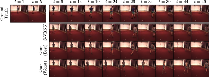
Figure 6: Conditioning frames and corresponding ground truth, best samples from StructVRNN and our method, and worst sample from our method, with respect to LPIPS, for a video of the Human3.6M dataset. Our method better captures the dynamic of the subject and produces less artefacts than StructVRNN.

KTH Action dataset (KTH).

This dataset is composed of real-world videos of people performing a single action per video in front of different backgrounds (Schüldt et al., 2004). Uncertainty lies in the appearance of subjects, the actions they perform, and how they are performed.

We substantially outperform on this dataset every considered baseline for each metric, as shown in Figures 4 and 1. In some videos, the subject only appears after the conditioning frames, requiring the model to sample the moment and location of the subject appearance, as well as its action. This critical case is illustrated in Figure 5. There, SVG fails to even generate a moving person; only SAVP and our model manage to do so, and our best sample is closer to the subject’s poses compared to SAVP. Moreover, the worst sample of our model demonstrates that it captures the diversity of the dataset by making a person appear at different time steps and with different speeds. An additional experiment on this dataset in Appendix G studies the influence of the encoder and decoder architecture on SVG and our model.

Finally, Table 1 and appendix Table 3 compare our method to its MLP and GRU alternative versions, leading to two conclusions. Firstly, it confirms the structural advantage of residual dynamics observed on Moving MNIST. Indeed, both MLP and GRU lose on all metrics, and especially in terms of realism according to LPIPS and FVD. Secondly, all three versions of our model (residual, MLP, GRU) outperform prior methods. Therefore, this improvement is due to their common inference method, latent nature and content variable, strengthening our motivation to propose a non-autoregressive model.

Human3.6M.

This dataset is also made of videos of subjects performing various actions (Ionescu et al., 2011, 2014). While there are more actions and details to capture with less training subjects than in KTH, the video backgrounds are less varied, and subjects always remain within the frames.

As reported in Figures 4 and 1, we significantly outperform, with respect to all considered metrics, StructVRNN, which is the state of the art on this dataset and has been shown to surpass both SAVP and SVG by Minderer et al. (2019). Figure 6 shows the dataset challenges; in particular, both methods do not capture well the subject appearance. Nonetheless, our model better captures its movements, and produces more realistic frames.

Comparisons to the MLP and GRU versions demonstrate once again the advantage of using residual dynamics. GRU obtains low scores on all metrics, which is coherent with similar results for SVG reported by Minderer et al. (2019). While the MLP version remains close to the residual model on PSNR, SSIM and LPIPS, it is largely beaten by the latter in terms of FVD.

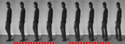
(a) Cropped KTH sample.

(b) Cropped Human3.6M sample.

(c) Cropped BAIR sample.

Figure 7: Generation examples at doubled or quadrupled frame rate, using a halved $\Delta t$ compared to training. Frames including a bottom red dashed bar are intermediate frames.

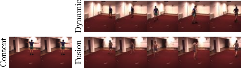
Figure 8: Video (bottom right) generated from the dynamic latent state $\bm{y}$ inferred with a video (top) and the content variable $\bm{w}$ computed with the conditioning frames of another video (left). The generated video keeps the same background as the bottom left frames, while the subject moves accordingly to the top frames.

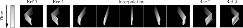
Figure 9: From left to right, $\bm{x}^{\mathrm{s}}$, $\widehat{\bm{x}}^{\mathrm{s}}$ (reconstruction of $\bm{x}^{\mathrm{s}}$ by the VAE of our model), results of the interpolation in the latent space between $\bm{x}^{\mathrm{s}}$ and $\bm{x}^{\mathrm{t}}$, $\widehat{\bm{x}}^{\mathrm{t}}$ and $\bm{x}^{\mathrm{t}}$. Each trajectory is materialized in shades of grey in the frames.

BAIR robot pushing dataset (BAIR).

This dataset contains videos of a Sawyer robotic arm pushing objects on a tabletop (Ebert et al., 2017). It is highly stochastic as the arm can change its direction at any moment. Our method achieves similar or better results compared to state-of-the-art models in terms of PSNR, SSIM and LPIPS, as shown in Figure 4, except for SV2P that produces very blurry samples, as seen in Appendix H, yielding good PSNR but prohibitive LPIPS scores. Our method obtains second-best FVD score, close to SAVP whose adversarial loss enables it to better model small objects, and outperforms SVG, whose variational architecture is closest to ours, demonstrating the advantage of non-autoregressive methods. Recent advances (Villegas et al., 2019) indicate that performance of such variational models can be improved by increasing networks capacities, but this is out of the scope of this paper.

Varying frame rate in testing.

We challenge here the ODE inspiration of our model. Equation 2 amounts to learning a residual function $f_{\bm{z}_{\lfloor t\rfloor+1}}$ over $t\in\left[\lfloor t\rfloor,\lfloor t\rfloor+1\right)$. We aim at testing whether this dynamics is close to its continuous generalization:

$$\dfrac{\operatorname{d\!}{}\bm{y}}{\operatorname{d\!}{t}}=f_{\bm{z}_{\lfloor t\rfloor+1}}\left(\bm{y}\right),$$ (9)

which is a piecewise ODE. To this end, we refine this Euler approximation during testing by halving $\Delta t$; if this maintains the performance of our model, then the dynamic rule of the latter is close to the piecewise ODE. As shown in Figures 4 and 1, prediction performances overall remain stable while generating twice as many frames (cf. Appendix F for further discussion). Therefore, the justification of the proposed update rule is supported by empirical evidence. This property can be used to generate videos at a higher frame rate, with the same model, and without supervision. We show in Figure 7 and Appendix F frames generated at a double and quadruple frame rate on KTH, Human3.6M and BAIR.

Disentangling dynamics and content.

Let us show that the proposed model actually separates content from dynamics as discussed in Section 3.2. To this end, two sequences $\bm{x}^{\mathrm{s}}$ and $\bm{x}^{\mathrm{t}}$ are drawn from the Human3.6M testing set. While $\bm{x}^{\mathrm{s}}$ is used for extracting our content variable $\bm{w}^{\mathrm{s}}$, dynamic states $\bm{y}^{\mathrm{t}}$ are inferred with our model from $\bm{x}^{\mathrm{t}}$. New frame sequences $\widehat{\bm{x}}$ are finally generated from the fusion of the content vector and the dynamics. This results in a content corresponding to the first sequence $\bm{x}^{\mathrm{s}}$ and a movement following the dynamics of the second sequence $\bm{x}^{\mathrm{t}}$, as observed in Figure 8. More samples for KTH, Human3.6M, and BAIR can be seen in Appendix H.

Interpolation of dynamics.

Our state-space structure allows us to learn semantic representations in $\bm{y}_{t}$. To highlight this feature, we test whether two deterministic Moving MNIST trajectories can be interpolated by linearly interpolating their inferred latent initial conditions. We begin by generating two trajectories $\bm{x}^{\mathrm{s}}$ and $\bm{x}^{\mathrm{t}}$ of a single moving digit. We infer their respective latent initial conditions $\bm{y}_{1}^{\mathrm{s}}$ and $\bm{y}_{1}^{\mathrm{t}}$. We then use our model to generate frame sequences from latent initial conditions linearly interpolated between $\bm{y}_{1}^{\mathrm{s}}$ and $\bm{y}_{1}^{\mathrm{t}}$. If it learned a meaningful latent space, the resulting trajectory should also be a smooth interpolation between the directions of reference trajectories $\bm{x}^{\mathrm{s}}$ and $\bm{x}^{\mathrm{t}}$, and this is what we observe in Figure 9. Additional examples can be found in Appendix H.

5 Conclusion

We introduce a novel dynamic latent model for stochastic video prediction which, unlike prior image-autoregressive models, decouples frame synthesis and dynamics. This temporal model is based on residual updates of a small latent state that is showed to perform better than RNN-based models. This endows our method with several desirable properties, such as temporal efficiency and latent space interpretability. We experimentally demonstrate the performance and advantages of the proposed model, which outperforms prior state-of-the-art methods for stochastic video prediction. This work is, to the best of our knowledge, the first to propose a latent dynamic model that scales for video prediction. The proposed model is also novel with respect to the recent line of work dealing with neural networks and ODEs for temporal modeling; it is the first such residual model to scale to complex stochastic data such as videos.

We believe that the general principles of our model (state-space, residual dynamic, static content variable) can be generally applied to other models as well. Interesting future works include replacing the VRNN of Minderer et al. (2019) with our residual dynamics in order to model the evolution of key-points, supplementing our model with more video-specific priors, or leveraging its state-space nature in model-based reinforcement learning.

Appendix A Evidence Lower Bound

We develop in this section the computations of the variational lower bound for the proposed model.

Using the original variational lower bound of Kingma & Welling (2014) in Equation 10:

$$\log p\left(\bm{x}_{1\mathrel{\mathop{\ordinarycolon}}T}\;\middle|\;\bm{w}\right)$$

$$\geq{} \mathbb{E}_{\left(\widetilde{\bm{z}}_{2\mathrel{\mathop{\ordinarycolon}}T},\widetilde{\bm{y}}_{1\mathrel{\mathop{\ordinarycolon}}T}\right)\sim q_{Z,Y}}\log p\left(\bm{x}_{1\mathrel{\mathop{\ordinarycolon}}T}\;\middle|\;\widetilde{\bm{z}}_{2\mathrel{\mathop{\ordinarycolon}}T},\widetilde{\bm{y}}_{1\mathrel{\mathop{\ordinarycolon}}T},\bm{w}\right)-D_{\mathrm{KL}}\left(q_{Z,Y}\;\middle\|\;p\left(\bm{y}_{1\mathrel{\mathop{\ordinarycolon}}T},\bm{z}_{2\mathrel{\mathop{\ordinarycolon}}T}\;\middle|\;\bm{w}\right)\right)$$ (10)

$$\begin{split}={}&\mathbb{E}_{\left(\widetilde{\bm{z}}_{2\mathrel{\mathop{\ordinarycolon}}T},\widetilde{\bm{y}}_{1\mathrel{\mathop{\ordinarycolon}}T}\right)\sim q_{Z,Y}}\log p\left(\bm{x}_{1\mathrel{\mathop{\ordinarycolon}}T}\;\middle|\;\widetilde{\bm{z}}_{2\mathrel{\mathop{\ordinarycolon}}T},\widetilde{\bm{y}}_{1\mathrel{\mathop{\ordinarycolon}}T},\bm{w}\right)-D_{\mathrm{KL}}\left(q\left(\bm{y}_{1},\bm{z}_{2\mathrel{\mathop{\ordinarycolon}}T}\;\middle|\;\bm{x}_{1\mathrel{\mathop{\ordinarycolon}}T}\right)\;\middle\|\;p\left(\bm{y}_{1},\bm{z}_{2\mathrel{\mathop{\ordinarycolon}}T}\right)\right)\end{split}$$ (11)

$$={} \mathbb{E}_{\left(\widetilde{\bm{z}}_{2\mathrel{\mathop{\ordinarycolon}}T},\widetilde{\bm{y}}_{1\mathrel{\mathop{\ordinarycolon}}T}\right)\sim q_{Z,Y}}\sum_{t=1}^{T}\log p\left(\bm{x}_{t}\;\middle|\;\widetilde{\bm{y}}_{t},\bm{w}\right)-D_{\mathrm{KL}}\left(q\left(\bm{y}_{1},\bm{z}_{2\mathrel{\mathop{\ordinarycolon}}T}\;\middle|\;\bm{x}_{1\mathrel{\mathop{\ordinarycolon}}T}\right)\;\middle\|\;p\left(\bm{y}_{1},\bm{z}_{2\mathrel{\mathop{\ordinarycolon}}T}\right)\right),$$ (12)

$$\log p\left(\bm{x}_{1\mathrel{\mathop{\ordinarycolon}}T}\;\middle|\;\bm{w}\right)$$

$$\begin{split}\geq{}&\mathbb{E}_{\left(\widetilde{\bm{z}}_{2\mathrel{\mathop{\ordinarycolon}}T},\widetilde{\bm{y}}_{1\mathrel{\mathop{\ordinarycolon}}T}\right)\sim q_{Z,Y}}\sum_{t=1}^{T}\log p\left(\bm{x}_{t}\;\middle|\;\widetilde{\bm{y}}_{t},\bm{w}\right)\\ &+\idotsint_{\bm{y}_{1},\bm{z}_{2\mathrel{\mathop{\ordinarycolon}}T}}q\left(\bm{y}_{1},\bm{z}_{2\mathrel{\mathop{\ordinarycolon}}T}\;\middle|\;\bm{x}_{1\mathrel{\mathop{\ordinarycolon}}T}\right)\log\frac{p\left(\bm{y}_{1},\bm{z}_{2\mathrel{\mathop{\ordinarycolon}}T}\right)}{q\left(\bm{y}_{1},\bm{z}_{2\mathrel{\mathop{\ordinarycolon}}T}\;\middle|\;\bm{x}_{1\mathrel{\mathop{\ordinarycolon}}T}\right)}\operatorname{d\!}\bm{z}_{2\mathrel{\mathop{\ordinarycolon}}T}\operatorname{d\!}\bm{y}_{1}\end{split}$$ (13)

$$\begin{split}={}&\mathbb{E}_{\left(\widetilde{\bm{z}}_{2\mathrel{\mathop{\ordinarycolon}}T},\widetilde{\bm{y}}_{1\mathrel{\mathop{\ordinarycolon}}T}\right)\sim q_{Z,Y}}\sum_{t=1}^{T}\log p\left(\bm{x}_{t}\;\middle|\;\widetilde{\bm{y}}_{t},\bm{w}\right)-D_{\mathrm{KL}}\left(q\left(\bm{y}_{1}\;\middle|\;\bm{x}_{1\mathrel{\mathop{\ordinarycolon}}T}\right)\;\middle\|\;p\left(\bm{y}_{1}\right)\right)\\ &+\mathbb{E}_{\widetilde{\bm{y}}_{1}\sim q\left(\bm{y}_{1}\;\middle|\;\bm{x}_{1\mathrel{\mathop{\ordinarycolon}}T}\right)}\left[\idotsint_{\bm{z}_{2\mathrel{\mathop{\ordinarycolon}}T}}q\left(\bm{z}_{2\mathrel{\mathop{\ordinarycolon}}T}\;\middle|\;\bm{x}_{1\mathrel{\mathop{\ordinarycolon}}T},\widetilde{\bm{y}}_{1}\right)\log\frac{p\left(\bm{z}_{2\mathrel{\mathop{\ordinarycolon}}T}\;\middle|\;\widetilde{\bm{y}}_{1}\right)}{q\left(\bm{z}_{2\mathrel{\mathop{\ordinarycolon}}T}\;\middle|\;\bm{x}_{1\mathrel{\mathop{\ordinarycolon}}T},\widetilde{\bm{y}}_{1}\right)}\operatorname{d\!}\bm{z}_{2\mathrel{\mathop{\ordinarycolon}}T}\right]\end{split}$$ (14)

$$\begin{split}={}&\mathbb{E}_{\left(\widetilde{\bm{z}}_{2\mathrel{\mathop{\ordinarycolon}}T},\widetilde{\bm{y}}_{1\mathrel{\mathop{\ordinarycolon}}T}\right)\sim q_{Z,Y}}\sum_{t=1}^{T}\log p\left(\bm{x}_{t}\;\middle|\;\widetilde{\bm{y}}_{t},\bm{w}\right)-D_{\mathrm{KL}}\left(q\left(\bm{y}_{1}\;\middle|\;\bm{x}_{1\mathrel{\mathop{\ordinarycolon}}k}\right)\;\middle\|\;p\left(\bm{y}_{1}\right)\right)\\ &+\mathbb{E}_{\widetilde{\bm{y}}_{1}\sim q\left(\bm{y}_{1}\;\middle|\;\bm{x}_{1\mathrel{\mathop{\ordinarycolon}}k}\right)}\left[\idotsint_{\bm{z}_{2\mathrel{\mathop{\ordinarycolon}}T}}q\left(\bm{z}_{2\mathrel{\mathop{\ordinarycolon}}T}\;\middle|\;\bm{x}_{1\mathrel{\mathop{\ordinarycolon}}T},\widetilde{\bm{y}}_{1}\right)\log\frac{p\left(\bm{z}_{2\mathrel{\mathop{\ordinarycolon}}T}\;\middle|\;\widetilde{\bm{y}}_{1}\right)}{q\left(\bm{z}_{2\mathrel{\mathop{\ordinarycolon}}T}\;\middle|\;\bm{x}_{1\mathrel{\mathop{\ordinarycolon}}T},\widetilde{\bm{y}}_{1}\right)}\operatorname{d\!}\bm{z}_{2\mathrel{\mathop{\ordinarycolon}}T}\right]\end{split}$$ (15)

$$\begin{split}={}&\mathbb{E}_{\left(\widetilde{\bm{z}}_{2\mathrel{\mathop{\ordinarycolon}}T},\widetilde{\bm{y}}_{1\mathrel{\mathop{\ordinarycolon}}T}\right)\sim q_{Z,Y}}\sum_{t=1}^{T}\log p\left(\bm{x}_{t}\;\middle|\;\widetilde{\bm{y}}_{t},\bm{w}\right)-D_{\mathrm{KL}}\left(q\left(\bm{y}_{1}\;\middle|\;\bm{x}_{1\mathrel{\mathop{\ordinarycolon}}k}\right)\;\middle\|\;p\left(\bm{y}_{1}\right)\right)\\ &+\mathbb{E}_{\widetilde{\bm{y}}_{1}\sim q\left(\bm{y}_{1}\;\middle|\;\bm{x}_{1\mathrel{\mathop{\ordinarycolon}}k}\right)}\left[\idotsint_{\bm{z}_{2\mathrel{\mathop{\ordinarycolon}}T}}\prod_{t=2}^{T}q\left(\bm{z}_{t}\;\middle|\;\bm{x}_{1\mathrel{\mathop{\ordinarycolon}}t}\right)\sum_{t=2}^{T}\log\frac{p\left(\bm{z}_{t}\;\middle|\;\widetilde{\bm{y}}_{1},\bm{z}_{2\mathrel{\mathop{\ordinarycolon}}t-1}\right)}{q\left(\bm{z}_{t}\;\middle|\;\bm{x}_{1\mathrel{\mathop{\ordinarycolon}}t}\right)}\operatorname{d\!}\bm{z}_{2\mathrel{\mathop{\ordinarycolon}}T}\right]\end{split}$$ (16)

$$\begin{split}={}&\mathbb{E}_{\left(\widetilde{\bm{z}}_{2\mathrel{\mathop{\ordinarycolon}}T},\widetilde{\bm{y}}_{1\mathrel{\mathop{\ordinarycolon}}T}\right)\sim q_{Z,Y}}\sum_{t=1}^{T}\log p\left(\bm{x}_{t}\;\middle|\;\widetilde{\bm{y}}_{t},\bm{w}\right)-D_{\mathrm{KL}}\left(q\left(\bm{y}_{1}\;\middle|\;\bm{x}_{1\mathrel{\mathop{\ordinarycolon}}k}\right)\;\middle\|\;p\left(\bm{y}_{1}\right)\right)\\ &-\mathbb{E}_{\widetilde{\bm{y}}_{1}\sim q\left(\bm{y}_{1}\;\middle|\;\bm{x}_{1\mathrel{\mathop{\ordinarycolon}}k}\right)}D_{\mathrm{KL}}\left(q\left(\bm{z}_{2}\;\middle|\;\bm{x}_{1\mathrel{\mathop{\ordinarycolon}}t}\right)\;\middle\|\;p\left(\bm{z}_{2}\;\middle|\;\widetilde{\bm{y}}_{1}\right)\right)\\ &+\mathbb{E}_{\widetilde{\bm{y}}_{1}\sim q\left(\bm{y}_{1}\;\middle|\;\bm{x}_{1\mathrel{\mathop{\ordinarycolon}}k}\right)}\mathbb{E}_{\widetilde{\bm{z}}_{2}\sim q\left(\bm{z}_{2}\;\middle|\;\bm{x}_{1\mathrel{\mathop{\ordinarycolon}}2}\right)}\left[\idotsint_{\bm{z}_{3\mathrel{\mathop{\ordinarycolon}}T}}\prod_{t=3}^{T}q\left(\bm{z}_{t}\;\middle|\;\bm{x}_{1\mathrel{\mathop{\ordinarycolon}}t}\right)\sum_{t=3}^{T}\log\frac{p\left(\bm{z}_{t}\;\middle|\;\bm{y}_{1},\widetilde{\bm{z}}_{2\mathrel{\mathop{\ordinarycolon}}t-1}\right)}{q\left(\bm{z}_{t}\;\middle|\;\bm{x}_{1\mathrel{\mathop{\ordinarycolon}}t}\right)}\operatorname{d\!}\bm{z}_{3\mathrel{\mathop{\ordinarycolon}}T}\right],\end{split}$$ (17)

$$\log p\left(\bm{x}_{1\mathrel{\mathop{\ordinarycolon}}T}\;\middle|\;\bm{w}\right)$$

$$\begin{split}\geq{}&\mathbb{E}_{\left(\widetilde{\bm{z}}_{2\mathrel{\mathop{\ordinarycolon}}T},\widetilde{\bm{y}}_{1\mathrel{\mathop{\ordinarycolon}}T}\right)\sim q_{Z,Y}}\sum_{t=1}^{T}\log p\left(\bm{x}_{t}\;\middle|\;\widetilde{\bm{y}}_{t},\bm{w}\right)-D_{\mathrm{KL}}\left(q\left(\bm{y}_{1}\;\middle|\;\bm{x}_{1\mathrel{\mathop{\ordinarycolon}}k}\right)\;\middle\|\;p\left(\bm{y}_{1}\right)\right)\\ &-\mathbb{E}_{\widetilde{\bm{y}}_{1}\sim q\left(\bm{y}_{1}\;\middle|\;\bm{x}_{\mathrm{c}}\right)}\left(\mathbb{E}_{\widetilde{\bm{z}}_{t}\sim q\left(\bm{z}_{t}\;\middle|\;\bm{x}_{1\mathrel{\mathop{\ordinarycolon}}t}\right)}\right)_{t=2}^{T}\sum_{t=2}^{T}D_{\mathrm{KL}}\left(q\left(\bm{z}_{t}\;\middle|\;\bm{x}_{1\mathrel{\mathop{\ordinarycolon}}t}\right)\;\middle\|\;p\left(\bm{z}_{t}\;\middle|\;\widetilde{\bm{y}}_{1},\widetilde{\bm{z}}_{1\mathrel{\mathop{\ordinarycolon}}t-1}\right)\right),\end{split}$$ (18)

and we finally retrieve Equation 7 by using the factorization of Equation 6:

$$\log p\left(\bm{x}_{1\mathrel{\mathop{\ordinarycolon}}T}\;\middle|\;\bm{w}\right)$$

$$\begin{split}\geq{}&\mathbb{E}_{\left(\widetilde{\bm{z}}_{2\mathrel{\mathop{\ordinarycolon}}T},\widetilde{\bm{y}}_{1\mathrel{\mathop{\ordinarycolon}}T}\right)\sim q_{Z,Y}}\sum_{t=1}^{T}\log p\left(\bm{x}_{t}\;\middle|\;\widetilde{\bm{y}}_{t},\bm{w}\right)-D_{\mathrm{KL}}\left(q\left(\bm{y}_{1}\;\middle|\;\bm{x}_{1\mathrel{\mathop{\ordinarycolon}}k}\right)\;\middle\|\;p\left(\bm{y}_{1}\right)\right)\\ &-\mathbb{E}_{\left(\widetilde{\bm{z}}_{2\mathrel{\mathop{\ordinarycolon}}T},\widetilde{\bm{y}}_{1\mathrel{\mathop{\ordinarycolon}}T}\right)\sim q_{Z,Y}}\sum_{t=2}^{T}D_{\mathrm{KL}}\left(q\left(\bm{z}_{t}\;\middle|\;\bm{x}_{1\mathrel{\mathop{\ordinarycolon}}t}\right)\;\middle\|\;p\left(\bm{z}_{t}\;\middle|\;\widetilde{\bm{y}}_{t-1}\right)\right).\end{split}$$ (19)

Appendix B Datasets Details

We detail in this section the datasets used in our experimental study.

B.1 Data Representation

For all datasets, video frames are represented by greyscale or RGB pixels with values within $\left[0,1\right]$ obtained by dividing by $255$ their original values lying in $\left\llbracket 0,255\right\rrbracket$.

B.2 Stochastic Moving MNIST

This monochrome dataset consists in one or two training MNIST digits (LeCun et al., 1998) of size $28\times 28$ moving linearly within a $64\times 64$ frame and randomly bouncing against its border, sampling a new direction and velocity at each bounce (Denton & Fergus, 2018). We use the same settings as Denton & Fergus (2018), train all models on $15$ timesteps, condition them at testing time on $5$ frames, and predict either $20$ (for the stochastic version) or $95$ (for the deterministic version) frames. Note that we adapted the dataset to sample more coherent bounces: the original dataset computes digit trajectories that are dependent on the chosen framerate, unlike our corrected version of the dataset. We consequently retrained SVG on this dataset, obtaining comparable results as those originally presented by Denton & Fergus (2018). Test data were produced by generating a trajectory for each testing digit, and randomly pairwise combining these trajectories to produce $5000$ testing sequences containing each two digits.

B.3 KTH Action Dataset (KTH)

This dataset is composed of real-world $64\times 64$ monochrome videos of $25$ people performing one of six actions (walking, jogging, running, boxing, handwaving and handclapping) in front of different backgrounds (Schüldt et al., 2004). Uncertainty lies in the appearance of subjects, the action they perform and how it is performed. We use the same settings as Denton & Fergus (2018), train all models on $20$ timesteps, condition them at testing time on $10$ frames, and predict $30$ frames. The training set is formed with actions from the first $20$ subjects, the remaining five being used for testing. Training is performed by sampling sub-sequences of size $20$ in the training set. The test set is composed of $1000$ randomly sampled sub-sequences of size $40$.

B.4 Human3.6M

This dataset is also made of videos of subjects performing various actions (Ionescu et al., 2011, 2014). While there are more actions and details to capture with less training subjects than in KTH, the video backgrounds are less varied, and subjects always remain within the frames. We use the same settings as Minderer et al. (2019) to train both our model and StructVRNN, for which there is no available pretrained model. We train all models on $16$ timesteps, condition them at testing time on $8$ frames, and predict $45$ frames. Videos used in our experiment are subsampled from the original videos at $6.25$Hz, center-cropped from $1000\times 1000$ to $800\times 800$ and resized to $64\times 64$ using the Lanczos filter of the Pillow library. The training set is composed of videos of subjects $1$, $5$, $6$, $7$, and $8$, and the testing set is made from subjects $9$ and $11$; videos showing more than one action, marked by “ALL” in the dataset, are excluded. Training is performed by sampling sub-sequences of size $16$ in the training set. The test set is composed of $1000$ randomly sampled sub-sequences of size $53$ from the testing videos.

B.5 BAIR Robot Pushing Dataset (BAIR)

This dataset contains $64\times 64$ videos of a Sawyer robotic arm pushing objects on a tabletop (Ebert et al., 2017). It is highly stochastic as the arm can change its direction at any moment. We use the same settings as Denton & Fergus (2018), train all models on $12$ timesteps, condition them at testing time on $2$ frames, and predict $28$ frames. Training and testing sets are the same as those used by Denton & Fergus (2018).

Appendix C Training Details

We expose in this section further information needed for the reproduction of our results.

C.1 Specifications

We used Python $3.7.6$ and PyTorch $1.4.0$ (Paszke et al., 2019) to implement our model. Each model was trained on Nvidia GPUs with CUDA $10.1$ using mixed-precision training (Micikevicius et al., 2018) with Apex.

C.2 Architecture

Encoder and decoder architecture.

Both $g_{\theta}$ and $h_{\phi}$ are chosen to have the same mirrored architecture that depends on the dataset. We used the same architectures as Denton & Fergus (2018): a DCGAN discriminator and generator architecture (Radford et al., 2016) for Moving MNIST, and a VGG16 (Simonyan & Zisserman, 2015) architecture (mirrored for $h_{\phi}$) for the other datasets. In both cases, the output of $h_{\phi}$ (i.e., $\widetilde{\bm{x}}$) is a vector of size $128$, and $g_{\theta}$ and $h_{\phi}$ weights are initialized using a centered Gaussian distribution with a standard deviation of $0.02$ (except for biases initialized to $0$, and batch normalization layers weights drawn from a Gaussian distribution with unit mean and a standard deviation of $0.02$). Additionally, we supplement $g_{\theta}$ with a last sigmoid activation in order to ensure its outputs lie within $\left[0,1\right]$ like the ground truth data.

Note that, during testing, predicted frames are directly generated by $g_{\theta}\left(\bm{y}_{t},\bm{w}\right)$ without sampling from the observation probability distribution ${\mathcal{G}}\left(g_{\theta}\left(\bm{y}_{t},\bm{w}\right)\right)={\mathcal{N}}\left(g_{\theta}\left(\bm{y}_{t},\bm{w}\right),\nu I\right)$. This is a common practice for Gaussian decoders in VAEs that is adopted by our competitors (Lee et al., 2018; Denton & Fergus, 2018; Minderer et al., 2019).

Content variable.

For the Moving MNIST dataset, the content variable $\bm{w}$ is obtained directly from $\widetilde{\bm{x}}$ and is a vector of size $128$. For KTH, Human3.6M, and BAIR, we supplement this vectorial variable with skip connections from all layers of the encoder $g_{\theta}$ that are then fed to the decoder $h_{\phi}$ to handle complex backgrounds. For Moving MNIST, the number of frames $k$ used to compute the content variable is $5$; for KTH and Human3.6M, it is $3$; for BAIR, it is $2$.

The vectorial content variable $\bm{w}$ is computed from $k$ input frames $\bm{x}_{\mathrm{c}}^{\left(k\right)}=\left(\bm{x}_{i_{1}},\ldots,\bm{x}_{i_{k}}\right)$ with $c_{\psi}$ defined as follows:

$$\bm{w}=c_{\psi}\left(\bm{x}_{\mathrm{c}}^{\left(k\right)}\right)=c_{\psi}^{2}\left(\sum_{j=1}^{k}c_{\psi}^{1}\left(\widetilde{\bm{x}}_{i_{j}}\right)\right).$$ (20)

In other words, $c_{\psi}$ transforms each frame representation using $c_{\psi}^{1}$, sums these transformations and outputs the application of $c_{\psi}^{2}$ to this sum. Since frame representations $\widetilde{\bm{x}}_{i_{j}}=h_{\phi}\left(\bm{x}_{i_{j}}\right)$ are computed independently from each other, $c_{\psi}$ is indeed permutation-invariant. In practice, $c_{\psi}^{1}$ consists in a linear layer of output size $256$ followed by a rectified linear unit (ReLU) activation, while $c_{\psi}^{2}$ is a linear layer of output size $256$ (making $\bm{w}$ of size $256$) followed by a hyperbolic tangent activation.

LSTM architecture.

The LSTM used for all datasets has a single layer of LSTM cells with a hidden state size of $256$.

MLP architecture.

All MLPs used in inference (with parameters $\phi$) have three linear layers with hidden size $256$ and ReLU activations. All MLPs used in the forward model (with parameters $\theta$) have four linear layers with hidden size 512 and ReLU activations. Any MLP outputting Gaussian distribution parameters $\left(\mu,\sigma\right)$ additionally includes a softplus (Dugas et al., 2001) applied to its output dimensions that are used to obtain $\sigma$. Weights of $f_{\theta}$ are orthogonally initialized with a gain of $1.2$ for KTH and Human3.6M, and $1.41$ for the other datasets (except for biases which are initialized to $0$), while the other MLPs are initialized with the default weight initialization of PyTorch.

Sizes of latent variables.

The sizes of the latent variables in our model are the following: for Moving MNIST, $\bm{y}$ and $\bm{z}$ have size $20$; for KTH, Human3.6M, and BAIR, $\bm{y}$ and $\bm{z}$ have size $50$.

Euler step size

Models are trained with $\Delta t=1$ on Moving MNIST, and with $\Delta t=\frac{1}{2}$ on the others datasets.

C.3 Optimization

Models are trained using the Adam optimizer (Kingma & Ba, 2015) with learning rate $3\text{\times}{10}^{-4}$, and decay rates $\beta_{1}=0.9$ and $\beta_{2}=0.999$.

Loss function.

The batch size is chosen to be $128$ for Moving MNIST, $100$ for KTH and Human3.6M, and $192$ for BAIR. The regularization coefficient $\lambda$ is always set to $1$. Logarithms used in the loss are natural logarithms.

For the Moving MNIST dataset, we follow Higgins et al. (2017) by weighting the KL divergence terms on $\bm{z}$ (i.e., the sum of KL divergences in Equation 7) with a multiplication factor $\beta=2$.

Variance of the observation.

The variance $\nu$ considered in the observation probability distribution ${\mathcal{G}}\left(g_{\theta}\left(\bm{y},\bm{w}\right)\right)={\mathcal{N}}\left(g_{\theta}\left(\bm{y}_{t},\bm{w}\right),\nu I\right)$ is chosen as follows:

• for Moving MNIST, $\nu=1$;

• for KTH and Human3.6M, $\nu=$ $4\text{\times}{10}^{-2}$;

• for BAIR, $\nu=\frac{1}{2}$.

Number of optimization steps.

The number of optimization steps for each dataset is the following:

• Stochastic Moving MNIST: $1\,000\,000$ steps, with additional $100\,000$ steps where the learning rate is linearly decreased to $0$;

• Deterministic Moving MNIST: $800\,000$ steps, with additional $100\,000$ steps where the learning rate is linearly decreased to $0$;

• KTH: $150\,000$ steps, with additional $50\,000$ steps where the learning rate is linearly decreased to $0$;

• Human3.6M: $325\,000$ steps, with additional $25\,000$ steps where the learning rate is linearly decreased to $0$;

• BAIR: $1\,000\,000$ steps, with additional $500\,000$ steps where the learning rate is linearly decreased to $0$.

Furthermore, the final models for KTH and Human3.6M are chosen among several checkpoints, computed every $5000$ iterations for KTH and $20\,000$ iterations for Human3.6M, as the ones obtaining the best evaluation PSNR. This evaluation score differs from the test score as we extract from the training set an evaluation set by randomly selecting $5\%$ of the training videos from the training set of each dataset. More precisely, the evaluation PSNR for a checkpoint is computed as the mean best prediction PSNR for $400$ (for KTH) or $200$ (for Human3.6M) randomly extracted sequences of length $30$ (for KTH) or $53$ (for Human3.6M) from the videos of the evaluation set.

Appendix D Additional Numerical Results

Table 2: Numerical results (mean and $95\%$-confidence interval) for PSNR and SSIM of tested methods on the two-digits Moving MNIST dataset. Bold scores indicate the best performing method for each metric and, where appropriate, scores whose means lie in the confidence interval of the best performing method.

Models	Stochastic		Deterministic
	PSNR	SSIM	PSNR	SSIM
SVG	$14.50$ p m 0.04	$0.7090$ p m 0.0015	$12.85$ p m 0.03	$0.6185$ p m 0.0011
Ours	$16.93$ p m 0.07	$0.7799$ p m 0.0020	$18.25$ p m 0.06	$0.8300$ p m 0.0017
Ours - MLP	$16.55$ p m 0.06	$0.7694$ p m 0.0019	$16.70$ p m 0.05	$0.7876$ p m 0.0015
Ours - GRU	$15.80$ p m 0.05	$0.7464$ p m 0.0016	$13.17$ p m 0.03	$0.6237$ p m 0.0011
Ours - w/o $\bm{z}$	—	—	$14.99$ p m 0.03	$0.4757$ p m 0.0019

Table 3: Numerical results (mean and $95\%$-confidence interval, when relevant) for PSNR, SSIM, and LPIPS of tested methods on the KTH dataset. Bold scores indicate the best performing method for each metric and, where appropriate, scores whose means lie in the confidence interval of the best performing method.

Models	PSNR	SSIM	LPIPS
SV2P	$28.19$ p m 0.31	$0.8141$ p m 0.0050	$0.2049$ p m 0.0053
SAVP	$26.51$ p m 0.29	$0.7564$ p m 0.0062	$0.1120$ p m 0.0039
SVG	$28.06$ p m 0.29	$0.8438$ p m 0.0054	$0.0923$ p m 0.0038
Ours	$29.69$ p m 0.32	$0.8697$ p m 0.0046	$0.0736$ p m 0.0029
Ours - $\frac{\Delta t}{2}$	$29.43$ p m 0.33	$0.8633$ p m 0.0049	$0.0790$ p m 0.0034
Ours - MLP	$28.91$ p m 0.34	$0.8527$ p m 0.0051	$0.0799$ p m 0.0032
Ours - GRU	$29.14$ p m 0.33	$0.8590$ p m 0.0050	$0.0790$ p m 0.0032

Table 4: Numerical results (mean and $95\%$-confidence interval, when relevant) for PSNR, SSIM, and LPIPS of tested methods on the Human3.6M dataset. Bold scores indicate the best performing method for each metric and, where appropriate, scores whose means lie in the confidence interval of the best performing method.

Models	PSNR	SSIM	LPIPS
StructVRNN	$24.46$ p m 0.17	$0.8868$ p m 0.0025	$0.0557$ p m 0.0013
Ours	$25.30$ p m 0.19	$0.9074$ p m 0.0022	$0.0509$ p m 0.0013
Ours - $\frac{\Delta t}{2}$	$25.14$ p m 0.21	$0.9049$ p m 0.0024	$0.0534$ p m 0.0015
Ours - MLP	$25.00$ p m 0.19	$0.9047$ p m 0.0021	$0.0529$ p m 0.0013
Ours - GRU	$23.54$ p m 0.18	$0.8868$ p m 0.0022	$0.0683$ p m 0.0014

Table 5: Numerical results (mean and $95\%$-confidence interval, when relevant) with respect to PSNR, SSIM, and LPIPS of tested methods on the BAIR dataset. Bold scores indicate the best performing method for each metric and, where appropriate, scores whose means lie in the confidence interval of the best performing method.

Models	PSNR	SSIM	LPIPS
SV2P	$20.39$ p m 0.27	$0.8169$ p m 0.0086	$0.0912$ p m 0.0053
SAVP	$18.44$ p m 0.25	$0.7887$ p m 0.0092	$0.0634$ p m 0.0026
SVG	$18.95$ p m 0.26	$0.8058$ p m 0.0088	$0.0609$ p m 0.0034
Ours	$19.59$ p m 0.27	$0.8196$ p m 0.0084	$0.0574$ p m 0.0032
Ours - $\frac{\Delta t}{2}$	$19.45$ p m 0.26	$0.8196$ p m 0.0082	$0.0579$ p m 0.0032
Ours - MLP	$19.56$ p m 0.26	$0.8194$ p m 0.0084	$0.0572$ p m 0.0032
Ours - GRU	$19.41$ p m 0.26	$0.8170$ p m 0.0084	$0.0585$ p m 0.0032

Tables 2, 3, 4 and 5 present, respectively, numerical results for PSNR, SSIM and LPIPS averaged over all time steps for our methods and considered baselines on the Moving MNIST, KTH, Human3.6M, and BAIR datasets, corresponding to Figures 3 and 4.

Note that we choose the learned prior version of SVG for all datasets but KTH, for which we choose the fixed prior version, as done by its authors (Denton & Fergus, 2018).

Appendix E Pendulum Experiments

We test the ability of our model to model the dynamics of a common dataset used in the literature of state-space models (Karl et al., 2017; Fraccaro et al., 2017), Pendulum (Karl et al., 2017). It consists of noisy observations of a dynamic torque-controlled pendulum; it is stochastic as the information of this control is not available. We test our model, without the content variable $\bm{w}$, in the same setting as DVBF (Karl et al., 2017) and KVAE (Fraccaro et al., 2017) and report the corresponding ELBO scores in Table 6. The encoders and decoders for all methods are MLPs.

Our model outperforms DVBF and is merely beaten by KVAE. This can be explained by the nature of the KVAE model, whose sequential model is learned using a Kalman filter rather than a VAE, allowing exact inference in the latent space. On the contrary, DVBF is learned, like our model, by a sequential VAE, and is thus closer to our model than KVAE. This result then shows that the dynamic model that we propose in the context of sequential VAEs is more adapted on this dataset than the one of DVBF, and achieve results close to a method taking advantage of exact inference using adapted tools such as Kalman filters.

Table 6: ELBO, in nats, achieved by DVBF, KVAE and our model on the Pendulum dataset. The bold score indicates the best performing method.

DVBF	KVAE	Ours
$798.56$	$807.02$	$806.12$

Appendix F Influence of the Euler step size

Table 7 details the numerical results of our model trained on BAIR with $\Delta t=\frac{1}{2}$ and tested with different values of $\Delta t$. It shows that, when refining the Euler approximation, our model maintains its performances in settings unseen during training.

Tables 8 and 9 detail the numerical results of our model trained on KTH with, respectively, $\Delta t=1$ and $\Delta t=\frac{1}{2}$, and tested with different values of $\Delta t$. They show that if $\Delta t$ is chosen too high when training (here, $\Delta t=1$), the model performance drops when refining the Euler approximation. We assume that this phenomenon arises because the Euler approximation used in training is too rough, making the model adapt to an overly discretized dynamic that cannot be transferred to smaller Euler step sizes. Indeed, when training with a smaller step size (here, $\Delta t=\frac{1}{2}$), results in the training settings are equivalent while results obtained with a lower $\Delta t$ are now much closer, if not equivalent, to the nominal ones. This shows that the model learns a continuous dynamic if learned with a small enough step size.

Note that the loss of performance using a higher $\Delta t$ in testing than in training, like in Tables 7 and 9, is expected as it corresponds to loosening the Euler approximation compared to training. However, even in this challenging setting, our model maintains state-of-the-art results, demonstrating the quality of the learned dynamic as it can be further discretized if needed at the cost of a reasonable drop in performance.

Table 7: Numerical results for PSNR, SSIM, and LPIPS on BAIR of our model trained with $\Delta t=\frac{1}{2}$ and tested with different values of $\Delta t$.

Step size $\Delta t$	PSNR	SSIM	LPIPS
$\Delta t=1$	$18.95$ p m 0.25	$0.8139$ p m 0.0081	$0.0640$ p m 0.0036
$\bm{\Delta t=}\frac{\bm{1}}{\bm{2}}$	$19.59$ p m 0.27	$0.8196$ p m 0.0084	$0.0574$ p m 0.0032
$\Delta t=\frac{1}{3}$	$19.49$ p m 0.25	$0.8201$ p m 0.0082	$0.0574$ p m 0.0032
$\Delta t=\frac{1}{4}$	$19.45$ p m 0.26	$0.8196$ p m 0.0082	$0.0579$ p m 0.0032
$\Delta t=\frac{1}{5}$	$19.46$ p m 0.26	$0.8197$ p m 0.0082	$0.0584$ p m 0.0032

Table 8: Numerical results for PSNR, SSIM, and LPIPS on KTH of our model trained with $\Delta t=1$ and tested with different values of $\Delta t$.

Step size $\Delta t$	PSNR	SSIM	LPIPS
$\bm{\Delta t=1}$	$29.77$ p m 0.33	$0.8681$ p m 0.0046	$0.0742$ p m 0.0029
$\Delta t=\frac{1}{2}$	$29.18$ p m 0.35	$0.8539$ p m 0.0054	$0.0882$ p m 0.0040
$\Delta t=\frac{1}{3}$	$29.05$ p m 0.36	$0.8509$ p m 0.0056	$0.0924$ p m 0.0043
$\Delta t=\frac{1}{4}$	$28.98$ p m 0.37	$0.8496$ p m 0.0057	$0.0939$ p m 0.0045
$\Delta t=\frac{1}{5}$	$28.95$ p m 0.37	$0.8490$ p m 0.0058	$0.0948$ p m 0.0045

Table 9: Numerical results for PSNR, SSIM, and LPIPS on KTH of our model trained with $\Delta t=\frac{1}{2}$ and tested with different values of $\Delta t$.

Step size $\Delta t$	PSNR	SSIM	LPIPS
$\Delta t=1$	$28.80$ p m 0.25	$0.8495$ p m 0.0053	$0.0994$ p m 0.0044
$\bm{\Delta t=}\frac{\bm{1}}{\bm{2}}$	$29.69$ p m 0.32	$0.8697$ p m 0.0046	$0.0736$ p m 0.0029
$\Delta t=\frac{1}{3}$	$29.52$ p m 0.33	$0.8656$ p m 0.0048	$0.0777$ p m 0.0033
$\Delta t=\frac{1}{4}$	$29.43$ p m 0.33	$0.8633$ p m 0.0049	$0.0790$ p m 0.0034
$\Delta t=\frac{1}{5}$	$29.35$ p m 0.34	$0.8615$ p m 0.0050	$0.0811$ p m 0.0036

Appendix G Autoregressivity and Impact of Encoder and Decoder Architecture

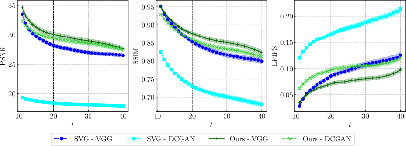
Figure 10: PNSR, SSIM and LPIPS scores with respect to $t$, with their $95\%$-confidence intervals, on the KTH dataset for SVG and our model with two choices of encoder and decoder architecture for each model: DCGAN and VGG. Vertical bars mark the length of training sequences.

Figures 10 and 10 expose the numerical results on KTH of our model trained with $\Delta t=1$ and SVG for two choices of encoder and decoder architectures: DCGAN and VGG.

Since DCGAN is a less powerful architecture than VGG, results of each method with VGG are expectedly better than those of the same method with DCGAN. Moreover, our model outperforms SVG for any fixed choice of encoder and decoder architecture, which is coherent with Figure 4.

We observe, however, that the difference between a method using VGG and its DCGAN counterpart differs depending on the model. Ours shows more robustness to the choice of encoder and decoder architecture, as it its performance decreases less than SVG when switching to a less powerful architecture. This loss is particularly pronounced with respect to PSNR, which is the metric that most penalizes dynamics errors. This shows that reducing the capacity of the encoders and decoders of SVG not only hurts its ability to produce realistic frames, as expected, but also substantially lowers its ability to learn a good dynamic. We assume that this phenomenon is caused by the autoregressive nature of SVG, which makes it reliant on the performance of its encoders and decoders. This supports our motivation to propose a non-autoregressive model for stochastic video prediction.

Table 10: FVD scores for SVG and our method on KTH, trained either with DCGAN or VGG encoders and decoders, with their $95\%$-confidence intervals over five different samples from the models.

SVG		Ours
VGG	DCGAN	VGG	DCGAN
$377$ p m 6	$542$ p m 6	$220$ p m 2	$371$ p m 3

Appendix H Additional Samples

This section includes additional samples corresponding to experiments described in Section 4.

H.1 Stochastic Moving MNIST

	Ground Truth
	SVG
	Ours (Best)
	Ours (Worst)
	Ours (Random)

Figure 11: Conditioning frames and corresponding ground truth and best samples with respect to PSNR from SVG and our method, and worst and random samples from our method, for an example of the Stochastic Moving MNIST dataset.

	Ground Truth
	SVG
	Ours (Best)
	Ours (Worst)
	Ours (Random)

Figure 12: Additional samples for the Stochastic Moving MNIST dataset (cf. Figure 11).

	Ground Truth
	SVG
	Ours (Best)
	Ours (Worst)
	Ours (Random)

Figure 13: Additional samples for the Stochastic Moving MNIST dataset (cf. Figure 11). SVG fails to maintain the shape of a digit, while ours is temporally coherent.

	Ground Truth
	SVG
	Ours (Best)
	Ours (Worst)
	Ours (Random)

Figure 14: Additional samples for the Stochastic Moving MNIST dataset (cf. Figure 11). This example was chosen in the worst $1\%$ testing examples of our model with respect to PSNR. Despite this adversarial criterion, our model maintains temporal consistency as digits are not deformed in the course of the video.

We present in Figures 11, 12, 13 and 14 additional samples from SVG and our model on Stochastic Moving MNIST.

In particular, Figure 13 shows SVG changing a digit shape in the course of a prediction even though it does not cross another digit, whereas ours maintain the digit shape. We assume that the advantage of our model comes from the latent nature of its dynamic and the use of a static content variable that is prevented from containing temporal information. Indeed, even when the best sample from our model is not close from the ground truth of the dataset, like in Figure 14, it still maintains the shapes of the digits.

H.2 KTH

	Ground Truth
	SV2P
	SVG
	SAVP
	Ours (Best)
	Ours (Worst)
	Ours (Random)

Figure 15: Conditioning frames and corresponding ground truth, best samples from SVG, SAVP and our method, and worst and random samples from our method, for an example of the KTH dataset. Samples are chosen according to their LPIPS with respect to the ground truth. On this specific task (clapping), all methods but SV2P (which produces blurry predictions) perform well, even though ours stays closer to the ground truth.

	Ground Truth
	SV2P
	SVG
	SAVP
	Ours (Best)
	Ours (Worst)
	Ours (Random)

Figure 16: Additional samples for the KTH dataset (cf. Figure 15). In this example, the shadow of the subject is visible in the last conditioning frames, foreshadowing its appearance. This is a failure case for SV2P and SVG which only produce an indistinct shadow, whereas SAVP and our model make the subject appear. Yet, SAVP produces the wrong action and an inconsistent subject in its best sample, while ours is correct.

	Ground Truth
	SV2P
	SVG
	SAVP
	Ours (Best)
	Ours (Worst)
	Ours (Random)

Figure 17: Additional samples for the KTH dataset (cf. Figure 15). This example is a failure case for all methods: SV2P produces blurry frames, SVG and SAVP are not consistent (change of action or subject appearance in the video), and our model produces a ghost image at the end of the prediction on the worst sample only.

	Ground Truth
	SV2P
	SVG
	SAVP
	Ours (Best)
	Ours (Worst)
	Ours (Random)

Figure 18: Additional samples for the KTH dataset (cf. Figure 15). Our model is the only one to make a subject appear, like in the ground truth.

	Ground Truth
	SV2P
	SVG
	SAVP
	Ours (Best)
	Ours (Worst)
	Ours (Random)

Figure 19: Additional samples for the KTH dataset (cf. Figure 15). The subject in this example is boxing, which is a challenging action in the dataset as all methods are far from the ground truth, even though ours remain closer in this case as well.

We present in Figures 15, 16, 17, 18 and 19 additional samples from SV2P, SVG, SAVP and our model on KTH, with additional insights.

H.3 Human3.6M

	Ground Truth
	S-VRNN
	Ours (Best)
	Ours (Worst)
	Ours (Random)

Figure 20: Conditioning frames and corresponding ground truth, best samples from StructVRNN and our method, and worst and random samples from our method, for an example of the Human3.6M dataset. Samples are chosen according to their LPIPS with respect to the ground truth. We better capture the movements of the subject as well as their diversity, predict more realistic subjects, and present frames with less artefacts.

	Ground Truth
	S-VRNN
	Ours (Best)
	Ours (Worst)
	Ours (Random)

Figure 21: Additional samples for the Human3.6M dataset (cf. Figure 20). This action is better captured by our model, which is able to produce diverse realistic predictions.

We present in Figures 20 and 21 additional samples from StructVRNN and our model on Human3.6M, with additional insights.

H.4 BAIR

	Ground Truth
	SV2P
	SVG
	SAVP
	Ours (Best)
	Ours (Worst)
	Ours (Random)

Figure 22: Conditioning frames and corresponding ground truth, best samples from SVG, SAVP and our method, and worst and random samples from our method, for an example of the BAIR dataset. Samples are chosen according to their LPIPS with respect to the ground truth.

	Ground Truth
	SV2P
	SVG
	SAVP
	Ours (Best)
	Ours (Worst)
	Ours (Random)

Figure 23: Additional samples for the BAIR dataset (cf. Figure 22).

	Ground Truth
	SV2P
	SVG
	SAVP
	Ours (Best)
	Ours (Worst)
	Ours (Random)

Figure 24: Additional samples for the BAIR dataset (cf. Figure 22).

We present in Figures 22, 23 and 24 additional samples from SV2P, SVG, SAVP and our model on BAIR.

H.5 Oversampling

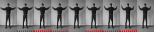
(a) Cropped KTH sample, centered on the subject.

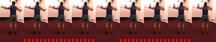
(b) Cropped Human3.6M sample, centered on the subject.

(c) Cropped BAIR sample, centered on the robot arm.

Figure 25: Generation examples at doubled or quadrupled frame rate, using a halved $\Delta t$ compared to training. Frames including a bottom red dashed bar are intermediate frames.

We present in Figure 25 additional examples of video generation at a doubled and quadrupled frame rate by our model.

H.6 Content Swap

		Dynamic
Content		Swap

Figure 26: Video (bottom right) generated from the combination of dynamic variables ($\bm{y}$, $\bm{z}$) inferred with a video (top) and a content variable ($\bm{w}$) computed with the conditioning frames of another video (bottom left).

		Dynamic
Content		Swap

Figure 27: Additional example of content swap (cf. Figure 26).

		Dynamic
Content		Swap

Figure 28: Additional example of content swap (cf. Figure 26). In this example, the extracted content is the video background, which is successfully transferred to the target video.

		Dynamic
Content		Swap

Figure 29: Additional example of content swap (cf. Figure 26). In this example, the extracted content is the video background and the subject appearance, which are successfully transferred to the target video.

		Dynamic
Content		Swap

Figure 30: Additional example of content swap (cf. Figure 26). This example shows a failure case of content swapping.

		Dynamic
Content		Swap

Figure 31: Additional example of content swap (cf. Figure 26).

We present in Figures 26, 27, 28, 29, 30 and 31 additional examples of content swap as in Figure 8.

H.7 Interpolation in the Latent Space

(a) Ref 1

(b) Rec 1

(c) Interpolation

(d) Rec 2

(e) Ref 2

Figure 32: From left to right, $\bm{x}^{\mathrm{s}}$, $\widehat{\bm{x}}^{\mathrm{s}}$ (reconstruction of $\bm{x}^{\mathrm{s}}$ by the VAE of our model), results of the interpolation in the latent space between $\bm{x}^{\mathrm{s}}$ and $\bm{x}^{\mathrm{t}}$, $\widehat{\bm{x}}^{\mathrm{t}}$ and $\bm{x}^{\mathrm{t}}$. Each trajectory is materialized in shades of grey in the frames.

(a) Ref 1

(b) Rec 1

(c) Interpolation

(d) Rec 2

(e) Ref 2

Figure 33: Additional example of interpolation in the latent space between two trajectories (cf. Figure 32).

We present in Figures 32 and 33 additional examples of interpolation in the latent space between two trajectories as in Figure 9.

References

- Babaeizadeh et al. (2018) Babaeizadeh, M., Finn, C., Erhan, D., Campbell, R., and Levine, S. Stochastic variational video prediction. In International Conference on Learning Representations, 2018.
- Bayer & Osendorfer (2014) Bayer, J. and Osendorfer, C. Learning stochastic recurrent networks. arXiv preprint arXiv:1411.7610, 2014.
- Behrmann et al. (2019) Behrmann, J., Grathwohl, W., Chen, R. T. Q., Duvenaud, D., and Jacobsen, J.-H. Invertible residual networks. In Chaudhuri, K. and Salakhutdinov, R. (eds.), Proceedings of the 36th International Conference on Machine Learning, volume 97 of Proceedings of Machine Learning Research, pp. 573–582, Long Beach, California, USA, June 2019. PMLR.
- Caballero et al. (2017) Caballero, J., Ledig, C., Aitken, A., Acosta, A., Totz, J., Wang, Z., and Shi, W. Real-time video super-resolution with spatio-temporal networks and motion compensation. In The IEEE Conference on Computer Vision and Pattern Recognition (CVPR), pp. 2848–2857, July 2017.
- Castrejon et al. (2019) Castrejon, L., Ballas, N., and Courville, A. Improved conditional VRNNs for video prediction. In The IEEE International Conference on Computer Vision (ICCV), pp. 7608–7617, October 2019.
- Chen et al. (2018) Chen, R. T. Q., Rubanova, Y., Bettencourt, J., and Duvenaud, D. Neural ordinary differential equations. In Bengio, S., Wallach, H., Larochelle, H., Grauman, K., Cesa-Bianchi, N., and Garnett, R. (eds.), Advances in Neural Information Processing Systems 31, pp. 6571–6583. Curran Associates, Inc., 2018.
- Cho et al. (2014) Cho, K., van Merriënboer, B., Gulcehre, C., Bahdanau, D., Bougares, F., Schwenk, H., and Bengio, Y. Learning phrase representations using RNN encoder-decoder for statistical machine translation. In Proceedings of the 2014 Conference on Empirical Methods in Natural Language Processing (EMNLP), pp. 1724–1734, Doha, Qatar, October 2014. Association for Computational Linguistics.
- Chung et al. (2015) Chung, J., Kastner, K., Dinh, L., Goel, K., Courville, A., and Bengio, Y. A recurrent latent variable model for sequential data. In Cortes, C., Lawrence, N. D., Lee, D. D., Sugiyama, M., and Garnett, R. (eds.), Advances in Neural Information Processing Systems 28, pp. 2980–2988. Curran Associates, Inc., 2015.
- De Brouwer et al. (2019) De Brouwer, E., Simm, J., Arany, A., and Moreau, Y. GRU-ODE-Bayes: Continuous modeling of sporadically-observed time series. In Wallach, H., Larochelle, H., Beygelzimer, A., d’Alché Buc, F., Fox, E., and Garnett, R. (eds.), Advances in Neural Information Processing Systems 32, pp. 7379–7390. Curran Associates, Inc., 2019.
- de Bézenac et al. (2019) de Bézenac, E., Ayed, I., and Gallinari, P. Optimal unsupervised domain translation. 2019.
- Denton & Birodkar (2017) Denton, E. and Birodkar, V. Unsupervised learning of disentangled representations from video. In Guyon, I., von Luxburg, U., Bengio, S., Wallach, H., Fergus, R., Vishwanathan, S. V. N., and Garnett, R. (eds.), Advances in Neural Information Processing Systems 30, pp. 4414–4423. Curran Associates, Inc., 2017.
- Denton & Fergus (2018) Denton, E. and Fergus, R. Stochastic video generation with a learned prior. In Dy, J. and Krause, A. (eds.), Proceedings of the 35th International Conference on Machine Learning, volume 80 of Proceedings of Machine Learning Research, pp. 1174–1183, Stockholmsmässan, Stockholm, Sweden, July 2018. PMLR.
- Dugas et al. (2001) Dugas, C., Bengio, Y., Bélisle, F., Nadeau, C., and Garcia, R. Incorporating second-order functional knowledge for better option pricing. In Leen, T. K., Dietterich, T. G., and Tresp, V. (eds.), Advances in Neural Information Processing Systems 13, pp. 472–478. MIT Press, 2001.
- Ebert et al. (2017) Ebert, F., Finn, C., Lee, A. X., and Levine, S. Self-supervised visual planning with temporal skip connections. In Levine, S., Vanhoucke, V., and Goldberg, K. (eds.), Proceedings of the 1st Annual Conference on Robot Learning, volume 78 of Proceedings of Machine Learning Research, pp. 344–356. PMLR, November 2017.
- Fan et al. (2019) Fan, H., Zhu, L., and Yang, Y. Cubic LSTMs for video prediction. In Proceedings of the AAAI Conference on Artificial Intelligence, volume 33, pp. 8263–8270, 2019.
- Finn et al. (2016) Finn, C., Goodfellow, I., and Levine, S. Unsupervised learning for physical interaction through video prediction. In Lee, D. D., Sugiyama, M., von Luxburg, U., Guyon, I., and Garnett, R. (eds.), Advances in Neural Information Processing Systems 29, pp. 64–72. Curran Associates, Inc., 2016.
- Fraccaro et al. (2016) Fraccaro, M., Sønderby, S. K., Paquet, U., and Winther, O. Sequential neural models with stochastic layers. In Lee, D. D., Sugiyama, M., von Luxburg, U., Guyon, I., and Garnett, R. (eds.), Advances in Neural Information Processing Systems 29, pp. 2199–2207. Curran Associates, Inc., 2016.
- Fraccaro et al. (2017) Fraccaro, M., Kamronn, S., Paquet, U., and Winther, O. A disentangled recognition and nonlinear dynamics model for unsupervised learning. In Guyon, I., von Luxburg, U., Bengio, S., Wallach, H., Fergus, R., Vishwanathan, S. V. N., and Garnett, R. (eds.), Advances in Neural Information Processing Systems 30, pp. 3601–3610. Curran Associates, Inc., 2017.
- Gao et al. (2019) Gao, H., Xu, H., Cai, Q.-Z., Wang, R., Yu, F., and Darrell, T. Disentangling propagation and generation for video prediction. In The IEEE International Conference on Computer Vision (ICCV), pp. 9006–9015, October 2019.
- Goodfellow (2016) Goodfellow, I. NIPS 2016 tutorial: Generative adversarial networks. arXiv preprint arXiv:1701.00160, 2016.
- Goodfellow et al. (2014) Goodfellow, I., Pouget-Abadie, J., Mirza, M., Xu, B., Warde-Farley, D., Ozair, S., Courville, A., and Bengio, Y. Generative adversarial nets. In Ghahramani, Z., Welling, M., Cortes, C., Lawrence, N. D., and Weinberger, K. Q. (eds.), Advances in Neural Information Processing Systems 27, pp. 2672–2680. Curran Associates, Inc., 2014.
- Graves (2013) Graves, A. Generating sequences with recurrent neural networks. arXiv preprint arXiv:1308.0850, 2013.
- Gregor et al. (2019) Gregor, K., Papamakarios, G., Besse, F., Buesing, L., and Weber, T. Temporal difference variational auto-encoder. In International Conference on Learning Representations, 2019.
- Hafner et al. (2019) Hafner, D., Lillicrap, T., Fischer, I., Villegas, R., Ha, D., Lee, H., and Davidson, J. Learning latent dynamics for planning from pixels. In Chaudhuri, K. and Salakhutdinov, R. (eds.), Proceedings of the 36th International Conference on Machine Learning, volume 97 of Proceedings of Machine Learning Research, pp. 2555–2565, Long Beach, California, USA, June 2019. PMLR.
- He et al. (2018) He, J., Lehrmann, A., Marino, J., Mori, G., and Sigal, L. Probabilistic video generation using holistic attribute control. In Ferrari, V., Hebert, M., Sminchisescu, C., and Weiss, Y. (eds.), The European Conference on Computer Vision (ECCV), pp. 466–483. Springer International Publishing, September 2018.
- He et al. (2016) He, K., Zhang, X., Ren, S., and Sun, J. Deep residual learning for image recognition. In The IEEE Conference on Computer Vision and Pattern Recognition (CVPR), pp. 770–778, June 2016.
- Higgins et al. (2017) Higgins, I., Matthey, L., Pal, A., Burgess, C., Glorot, X., Botvinick, M., Mohamed, S., and Lerchner, A. -VAE: Learning basic visual concepts with a constrained variational framework. In International Conference on Learning Representations, 2017.
- Hochreiter & Schmidhuber (1997) Hochreiter, S. and Schmidhuber, J. Long short-term memory. Neural Computation, 9(8):1735–1780, 1997.
- Ionescu et al. (2011) Ionescu, C., Li, F., and Sminchisescu, C. Latent structured models for human pose estimation. In 2011 International Conference on Computer Vision, pp. 2220–2227, November 2011.
- Ionescu et al. (2014) Ionescu, C., Papava, D., Olaru, V., and Sminchisescu, C. Human3.6M: Large scale datasets and predictive methods for 3D human sensing in natural environments. IEEE Transactions on Pattern Analysis and Machine Intelligence, 36(7):1325–1339, July 2014.
- Jia et al. (2016) Jia, X., De Brabandere, B., Tuytelaars, T., and Van Gool, L. Dynamic filter networks. In Lee, D. D., Sugiyama, M., von Luxburg, U., Guyon, I., and Garnett, R. (eds.), Advances in Neural Information Processing Systems 29, pp. 667–675. Curran Associates, Inc., 2016.
- Jiang et al. (2018) Jiang, H., Sun, D., Jampani, V., Yang, M.-H., Learned-Miller, E., and Kautz, J. Super SloMo: High quality estimation of multiple intermediate frames for video interpolation. In The IEEE Conference on Computer Vision and Pattern Recognition (CVPR), pp. 9000–9008, June 2018.
- Jin et al. (2020) Jin, B., Hu, Y., Tang, Q., Niu, J., Shi, Z., Han, Y., and Li, X. Exploring spatial-temporal multi-frequency analysis for high-fidelity and temporal-consistency video prediction. In IEEE/CVF Conference on Computer Vision and Pattern Recognition (CVPR), pp. 4554–4563, June 2020.
- Kalchbrenner et al. (2017) Kalchbrenner, N., van den Oord, A., Simonyan, K., Danihelka, I., Vinyals, O., Graves, A., and Kavukcuoglu, K. Video pixel networks. In Precup, D. and Teh, Y. W. (eds.), Proceedings of the 34th International Conference on Machine Learning, volume 70 of Proceedings of Machine Learning Research, pp. 1771–1779, International Convention Centre, Sydney, Australia, August 2017. PMLR.
- Karl et al. (2017) Karl, M., Soelch, M., Bayer, J., and van der Smagt, P. Deep variational Bayes filters: Unsupervised learning of state space models from raw data. In International Conference on Learning Representations, 2017.
- Kingma & Ba (2015) Kingma, D. P. and Ba, J. Adam: A method for stochastic optimization. In International Conference on Learning Representations, 2015.
- Kingma & Dhariwal (2018) Kingma, D. P. and Dhariwal, P. Glow: Generative flow with invertible 1x1 convolutions. In Bengio, S., Wallach, H., Larochelle, H., Grauman, K., Cesa-Bianchi, N., and Garnett, R. (eds.), Advances in Neural Information Processing Systems 31, pp. 10215–10224. Curran Associates, Inc., 2018.
- Kingma & Welling (2014) Kingma, D. P. and Welling, M. Auto-encoding variational Bayes. In International Conference on Learning Representations, 2014.
- Krishnan et al. (2017) Krishnan, R. G., Shalit, U., and Sontag, D. Structured inference networks for nonlinear state space models. In Proceedings of the AAAI Conference on Artificial Intelligence, volume 31, pp. 2101–2109, 2017.
- Kullback & Leibler (1951) Kullback, S. and Leibler, R. A. On information and sufficiency. The Annals of Mathematical Statistics, 22(1):79–86, 1951.
- Kumar et al. (2020) Kumar, M., Babaeizadeh, M., Erhan, D., Finn, C., Levine, S., Dinh, L., and Kingma, D. VideoFlow: A conditional flow-based model for stochastic video generation. In International Conference on Learning Representations, 2020.
- Le Guen & Thome (2020) Le Guen, V. and Thome, N. Disentangling physical dynamics from unknown factors for unsupervised video prediction. In The IEEE/CVF Conference on Computer Vision and Pattern Recognition (CVPR), pp. 11474–11484, June 2020.
- LeCun et al. (1998) LeCun, Y., Bottou, L., Bengio, Y., and Haffner, P. Gradient-based learning applied to document recognition. Proceedings of the IEEE, 86(11):2278–2324, November 1998.
- Lee et al. (2018) Lee, A. X., Zhang, R., Ebert, F., Abbeel, P., Finn, C., and Levine, S. Stochastic adversarial video prediction. arXiv preprint arXiv:1804.01523, 2018.
- Liang et al. (2017) Liang, X., Lee, L., Dai, W., and Xing, E. P. Dual motion GAN for future-flow embedded video prediction. In The IEEE International Conference on Computer Vision (ICCV), pp. 1762–1770, October 2017.
- Liu et al. (2017) Liu, Z., Yeh, R. A., Tang, X., Liu, Y., and Agarwala, A. Video frame synthesis using deep voxel flow. In The IEEE International Conference on Computer Vision (ICCV), pp. 4473–4481, October 2017.
- Liu et al. (2019) Liu, Z., Wu, J., Xu, Z., Sun, C., Murphy, K., Freeman, W. T., and Tenenbaum, J. B. Modeling parts, structure, and system dynamics via predictive learning. In International Conference on Learning Representations, 2019.
- Long et al. (2018) Long, Z., Lu, Y., Ma, X., and Dong, B. PDE-net: Learning PDEs from data. In Dy, J. and Krause, A. (eds.), Proceedings of the 35th International Conference on Machine Learning, volume 80 of Proceedings of Machine Learning Research, pp. 3208–3216, Stockholmsmässan, Stockholm Sweden, July 2018. PMLR.
- Lotter et al. (2017) Lotter, W., Kreiman, G., and Cox, D. Deep predictive coding networks for video prediction and unsupervised learning. In International Conference on Learning Representations, 2017.
- Lu et al. (2017a) Lu, C., Hirsch, M., and Schölkopf, B. Flexible spatio-temporal networks for video prediction. In The IEEE Conference on Computer Vision and Pattern Recognition (CVPR), pp. 2137–2145, July 2017a.
- Lu et al. (2017b) Lu, Y., Zhong, A., Li, Q., and Dong, B. Beyond finite layer neural networks: Bridging deep architectures and numerical differential equations. arXiv preprint arXiv:1710.10121, 2017b.
- Mathieu et al. (2016) Mathieu, M., Couprie, C., and LeCun, Y. Deep multi-scale video prediction beyond mean square error. In International Conference on Learning Representations, 2016.
- Micikevicius et al. (2018) Micikevicius, P., Narang, S., Alben, J., Diamos, G., Elsen, E., Garcia, D., Ginsburg, B., Houston, M., Kuchaiev, O., Venkatesh, G., and Wu, H. Mixed precision training. In International Conference on Learning Representations, 2018.
- Minderer et al. (2019) Minderer, M., Sun, C., Villegas, R., Cole, F., Murphy, K., and Lee, H. Unsupervised learning of object structure and dynamics from videos. In Wallach, H., Larochelle, H., Beygelzimer, A., d’Alché Buc, F., Fox, E., and Garnett, R. (eds.), Advances in Neural Information Processing Systems 32, pp. 92–102. Curran Associates, Inc., 2019.
- Paszke et al. (2019) Paszke, A., Gross, S., Massa, F., Lerer, A., Bradbury, J., Chanan, G., Killeen, T., Lin, Z., Gimelshein, N., Antiga, L., Desmaison, A., Kopf, A., Yang, E., DeVito, Z., Raison, M., Tejani, A., Chilamkurthy, S., Steiner, B., Fang, L., Bai, J., and Chintala, S. PyTorch: An imperative style, high-performance deep learning library. In Wallach, H., Larochelle, H., Beygelzimer, A., d’Alché Buc, F., Fox, E., and Garnett, R. (eds.), Advances in Neural Information Processing Systems 32, pp. 8026–8037. Curran Associates, Inc., 2019.
- Radford et al. (2016) Radford, A., Metz, L., and Chintala, S. Unsupervised representation learning with deep convolutional generative adversarial networks. In International Conference on Learning Representations, 2016.
- Ranzato et al. (2014) Ranzato, M., Szlam, A., Bruna, J., Mathieu, M., Collobert, R., and Chopra, S. Video (language) modeling: a baseline for generative models of natural videos. arXiv preprint arXiv:1412.6604, 2014.
- Rezende et al. (2014) Rezende, D. J., Mohamed, S., and Wierstra, D. Stochastic backpropagation and approximate inference in deep generative models. In Xing, E. P. and Jebara, T. (eds.), Proceedings of the 31st International Conference on Machine Learning, volume 32 of Proceedings of Machine Learning Research, pp. 1278–1286, Bejing, China, June 2014. PMLR.
- Ronneberger et al. (2015) Ronneberger, O., Fischer, P., and Brox, T. U-net: Convolutional networks for biomedical image segmentation. In Navab, N., Hornegger, J., Wells, W. M., and Frangi, A. F. (eds.), Medical Image Computing and Computer-Assisted Intervention – MICCAI 2015, pp. 234–241, Cham, 2015. Springer International Publishing.
- Rousseau et al. (2019) Rousseau, F., Drumetz, L., and Fablet, R. Residual networks as flows of diffeomorphisms. Journal of Mathematical Imaging and Vision, May 2019.
- Rubanova et al. (2019) Rubanova, Y., Chen, R. T. Q., and Duvenaud, D. Latent ordinary differential equations for irregularly-sampled time series. In Wallach, H., Larochelle, H., Beygelzimer, A., d’Alché Buc, F., Fox, E., and Garnett, R. (eds.), Advances in Neural Information Processing Systems 32, pp. 5320–5330. Curran Associates, Inc., 2019.
- Rumelhart et al. (1988) Rumelhart, D. E., Hinton, G. E., and Williams, R. J. Neurocomputing: Foundations of Research, chapter Learning Representations by Back-Propagating Errors, pp. 696–699. MIT Press, Cambridge, MA, USA, 1988.
- Ryder et al. (2018) Ryder, T., Golightly, A., McGough, A. S., and Prangle, D. Black-box variational inference for stochastic differential equations. In Dy, J. and Krause, A. (eds.), Proceedings of the 35th International Conference on Machine Learning, volume 80 of Proceedings of Machine Learning Research, pp. 4423–4432, Stockholmsmässan, Stockholm Sweden, July 2018. PMLR.
- Santoro et al. (2017) Santoro, A., Raposo, D., Barrett, D. G. T., Malinowski, M., Pascanu, R., Battaglia, P., and Lillicrap, T. A simple neural network module for relational reasoning. In Guyon, I., von Luxburg, U., Bengio, S., Wallach, H., Fergus, R., Vishwanathan, S. V. N., and Garnett, R. (eds.), Advances in Neural Information Processing Systems 30, pp. 4967–4976. Curran Associates, Inc., 2017.
- Schüldt et al. (2004) Schüldt, C., Laptev, I., and Caputo, B. Recognizing human actions: A local SVM approach. In Proceedings of the 17th International Conference on Pattern Recognition, 2004. ICPR 2004., volume 3, pp. 32–36, August 2004.
- Shi et al. (2015) Shi, X., Chen, Z., Wang, H., Yeung, D.-Y., Wong, W.-k., and Woo, W.-c. Convolutional LSTM network: A machine learning approach for precipitation nowcasting. In Cortes, C., Lawrence, N. D., Lee, D. D., Sugiyama, M., and Garnett, R. (eds.), Advances in Neural Information Processing Systems 28, pp. 802–810. Curran Associates, Inc., 2015.
- Simonyan & Zisserman (2015) Simonyan, K. and Zisserman, A. Very deep convolutional networks for large-scale image recognition. In International Conference on Learning Representations, 2015.
- Srivastava et al. (2015) Srivastava, N., Mansimov, E., and Salakhudinov, R. Unsupervised learning of video representations using LSTMs. In Bach, F. and Blei, D. (eds.), Proceedings of the 32nd International Conference on Machine Learning, volume 37 of Proceedings of Machine Learning Research, pp. 843–852, Lille, France, July 2015. PMLR.
- Tulyakov et al. (2018) Tulyakov, S., Liu, M.-Y., Yang, X., and Kautz, J. MoCoGAN: Decomposing motion and content for video generation. In The IEEE Conference on Computer Vision and Pattern Recognition (CVPR), pp. 1526–1535, June 2018.
- Unterthiner et al. (2018) Unterthiner, T., van Steenkiste, S., Kurach, K., Marinier, R., Michalski, M., and Gelly, S. Towards accurate generative models of video: A new metric & challenges. arXiv preprint arXiv:1812.01717, 2018.
- van den Oord et al. (2016) van den Oord, A., Kalchbrenner, N., Espeholt, L., Kavukcuoglu, K., Vinyals, O., and Graves, A. Conditional image generation with PixelCNN decoders. In Lee, D. D., Sugiyama, M., von Luxburg, U., Guyon, I., and Garnett, R. (eds.), Advances in Neural Information Processing Systems 29, pp. 4790–4798. Curran Associates, Inc., 2016.
- van Steenkiste et al. (2018) van Steenkiste, S., Chang, M., Greff, K., and Schmidhuber, J. Relational neural expectation maximization: Unsupervised discovery of objects and their interactions. In International Conference on Learning Representations, 2018.
- Villegas et al. (2017) Villegas, R., Yang, J., Hong, S., Lin, X., and Lee, H. Decomposing motion and content for natural video sequence prediction. In International Conference on Learning Representations, 2017.
- Villegas et al. (2019) Villegas, R., Pathak, A., Kannan, H., Erhan, D., Le, Q. V., and Lee, H. High fidelity video prediction with large stochastic recurrent neural networks. In Wallach, H., Larochelle, H., Beygelzimer, A., d’Alché Buc, F., Fox, E., and Garnett, R. (eds.), Advances in Neural Information Processing Systems 32, pp. 81–91. Curran Associates, Inc., 2019.
- Vondrick & Torralba (2017) Vondrick, C. and Torralba, A. Generating the future with adversarial transformers. In The IEEE Conference on Computer Vision and Pattern Recognition (CVPR), pp. 2992–3000, July 2017.
- Walker et al. (2015) Walker, J., Gupta, A., and Hebert, M. Dense optical flow prediction from a static image. In The IEEE International Conference on Computer Vision (ICCV), pp. 2443–2451, December 2015.
- Walker et al. (2016) Walker, J., Doersch, C., Gupta, A., and Hebert, M. An uncertain future: Forecasting from static images using variational autoencoders. In Leibe, B., Matas, J., Sebe, N., and Welling, M. (eds.), The European Conference on Computer Vision (ECCV), pp. 835–851. Springer International Publishing, October 2016.
- Wang et al. (2018) Wang, T.-C., Liu, M.-Y., Zhu, J.-Y., Liu, G., Tao, A., Kautz, J., and Catanzaro, B. Video-to-video synthesis. In Bengio, S., Wallach, H., Larochelle, H., Grauman, K., Cesa-Bianchi, N., and Garnett, R. (eds.), Advances in Neural Information Processing Systems 31, pp. 1144–1156. Curran Associates, Inc., 2018.
- Weissenborn et al. (2020) Weissenborn, D., Täckström, O., and Uszkoreit, J. Scaling autoregressive video models. In International Conference on Learning Representations, 2020.
- Wichers et al. (2018) Wichers, N., Villegas, R., Erhan, D., and Lee, H. Hierarchical long-term video prediction without supervision. In Dy, J. and Krause, A. (eds.), Proceedings of the 35th International Conference on Machine Learning, volume 80 of Proceedings of Machine Learning Research, pp. 6038–6046, Stockholmsmässan, Stockholm Sweden, July 2018. PMLR.
- Wu et al. (2020) Wu, Y., Gao, R., Park, J., and Chen, Q. Future video synthesis with object motion prediction. In IEEE/CVF Conference on Computer Vision and Pattern Recognition (CVPR), pp. 5539–5548, June 2020.
- Xu et al. (2018a) Xu, J., Ni, B., Li, Z., Cheng, S., and Yang, X. Structure preserving video prediction. In The IEEE Conference on Computer Vision and Pattern Recognition (CVPR), pp. 1460–1469, June 2018a.
- Xu et al. (2018b) Xu, J., Ni, B., and Yang, X. Video prediction via selective sampling. In Bengio, S., Wallach, H., Larochelle, H., Grauman, K., Cesa-Bianchi, N., and Garnett, R. (eds.), Advances in Neural Information Processing Systems 31, pp. 1705–1715. Curran Associates, Inc., 2018b.
- Xue et al. (2016) Xue, T., Wu, J., Bouman, K. L., and Freeman, W. T. Visual dynamics: Probabilistic future frame synthesis via cross convolutional networks. In Lee, D. D., Sugiyama, M., von Luxburg, U., Guyon, I., and Garnett, R. (eds.), Advances in Neural Information Processing Systems 29, pp. 91–99. Curran Associates, Inc., 2016.
- Yingzhen & Mandt (2018) Yingzhen, L. and Mandt, S. Disentangled sequential autoencoder. In Dy, J. and Krause, A. (eds.), Proceedings of the 35th International Conference on Machine Learning, volume 80 of Proceedings of Machine Learning Research, pp. 5670–5679, Stockholmsmässan, Stockholm Sweden, July 2018. PMLR.
- Yıldız et al. (2019) Yıldız, C., Heinonen, M., and Lahdesmaki, H. ODE2VAE: Deep generative second order odes with Bayesian neural networks. In Wallach, H., Larochelle, H., Beygelzimer, A., d’Alché Buc, F., Fox, E., and Garnett, R. (eds.), Advances in Neural Information Processing Systems 32, pp. 13412–13421. Curran Associates, Inc., 2019.
- Zaheer et al. (2017) Zaheer, M., Kottur, S., Ravanbakhsh, S., Póczos, B., Salakhutdinov, R., and Smola, A. J. Deep sets. In Guyon, I., von Luxburg, U., Bengio, S., Wallach, H., Fergus, R., Vishwanathan, S. V. N., and Garnett, R. (eds.), Advances in Neural Information Processing Systems 30, pp. 3391–3401. Curran Associates, Inc., 2017.
- Zhang et al. (2018) Zhang, R., Isola, P., Efros, A. A., Shechtman, E., and Wang, O. The unreasonable effectiveness of deep features as a perceptual metric. In The IEEE Conference on Computer Vision and Pattern Recognition (CVPR), pp. 586–595, June 2018.