Numerical solution of the dynamical mean field theory
of infinite-dimensional equilibrium liquids

Abstract

We present a numerical solution of the dynamical mean field theory of infinite-dimensional equilibrium liquids established in [Phys. Rev. Lett. 116, 015902 (2016)]. For soft sphere interactions, we obtain the numerical solution by an iterative algorithm and a straightforward discretization of time. We also discuss the case of hard spheres, for which we first derive analytically the dynamical mean field theory as a non-trivial limit of that of soft spheres. We present numerical results for the memory function and the mean square displacement. Our results reproduce and extend kinetic theory in the dilute or short-time limit, while they also describe dynamical arrest towards the glass phase in the dense strongly-interacting regime.

I Introduction

Solving the dynamics of dense equilibrium liquids is a notoriously difficult problem Hansen and McDonald (1986). In the low-density limit, or at short times, the solution is obtained via kinetic theory, which allows one to obtain microscopic expressions for the correlation functions and transport coefficients, while at any density, hydrodynamics provides a description of the dynamics at large length and time scales taking the transport coefficients as input. However, at high densities or low temperatures, kinetic theory breaks down, and the hydrodynamic regime is pushed to scales that are much larger than any experimentally relevant scale. In this strongly interacting “supercooled liquid” regime, dynamics is slow, viscosity is high, and both correlation functions and transport coefficients display non-trivial behavior that is not captured by kinetic theory. The only microscopic description of this regime is obtained by the Mode-Coupling Theory (MCT) Bengtzelius et al. (1984); Götze (2008), which is a set of closed equations derived from a series of poorly controlled approximations of the true dynamics. Despite its non-systematic nature Das and Mazenko (1986); Andreanov et al. (2006); Kim and Kawasaki (2007); Jacquin and Van Wijland (2011), MCT accurately describes the initial slowing down of liquid dynamics upon supercooling, including the wavevector dependence of correlation functions Götze (1999).

Interestingly, in the formal limit in which the spatial dimension $d$ goes to infinity, liquid thermodynamics reduces to the calculation of the second virial coefficient Frisch et al. (1985); Frisch and Percus (1987); Wyler et al. (1987); Frisch and Percus (1999). Based on this observation, a first attempt to solve exactly liquid dynamics for $d\rightarrow\infty$ was presented in Kirkpatrick and Wolynes (1987) (see also Elskens and Frisch (1988)), but the full dynamical mean field theory (DMFT) that describes exactly the equilibrium dynamics in $d\rightarrow\infty$ was only derived recently, via a second-order virial expansion on trajectories Maimbourg et al. (2016) or via a dynamic cavity method Szamel (2017); Agoritsas et al. (2018); Agoritsas et al. (2019a). The DMFT provides a set of closed one-dimensional integro-differential equations, which exactly describe the many-body liquid dynamics in the thermodynamic limit, and are similar in structure to those obtained for quantum systems in the same limit Georges et al. (1996). We refer the reader to Charbonneau et al. (2017); Agoritsas et al. (2019a, b); Parisi et al. (2020) for a detailed review of the solution of liquid dynamics in infinite dimensions, including its extension to the out-of-equilibrium setting (see also de Pirey et al. (2019) for a related approach).

Unfortunately, the analytical solution of the DMFT equations is out of reach. In this work, we present their numerical solution, obtained through an iterative method and a straightforward discretization of time. This strategy, however, only works for differentiable interaction potentials. We thus discuss how to derive the DMFT of hard spheres via a non-trivial limit of a soft sphere interaction. We present numerical results for soft and hard spheres, supported by analytical computations at low densities, in the short time limit, and at long times in the glass phase.

The paper is organized as follows. In section II we review the basic equations of the DMFT of liquids. In section III, we discuss the hard sphere limit of DMFT. In section IV, we discuss the discretization and convergence algorithms used in this work. In section V, we present the numerical solution for soft and hard spheres. Finally, in section VI we draw our conclusions and present some perspectives for future work. A few technical discussions are presented in Appendix. Note that the theoretical analysis developed in sections II and III and the numerical methods and results reported in sections IV and V can also be read independently; we present them jointly for the sake of completeness.

II Dynamical mean field theory

II.1 General formulation

In the following, we consider a liquid of interacting particles in $d$ dimensions, with pair interaction potential $v(r)$ having a typical interaction scale $\ell$, at temperature $T$ and number density $\rho$ in the thermodynamic limit. We denote by $\widehat{\varphi}=2^{d}\varphi/d=\rho V_{d}\ell^{d}/d$ the scaled packing fraction, where $V_{d}=\pi^{d/2}/\Gamma(1+d/2)$ is the volume of a unit sphere in $d$ dimensions. In the infinite dimensional limit, it is convenient to describe the dynamics in terms of the inter-particle gap $h=d(r/\ell-1)$, defining as well the rescaled potential $\bar{v}(h)=v[\ell(1+h/d)]$, which is assumed to have a finite limit when $d\rightarrow\infty$ Parisi et al. (2020).

In the most general case, we consider the Langevin dynamics of the system, being $\widehat{m}=(\ell^{2}/2d^{2})m$ and $\widehat{\zeta}=(\ell^{2}/2d^{2})\zeta$ respectively the scaled mass and friction coefficient, which are kept finite in the limit $d\rightarrow\infty$ in order to obtain a non-trivial dynamics Maimbourg et al. (2016); Agoritsas et al. (2019a); Parisi et al. (2020). Denoting a time derivative by a dot, $\dot{h}(t)=\mathrm{d}h/\mathrm{d}t$, DMFT leads to the following set of self-consistent equations, which describe exactly the equilibrium dynamics when $d\rightarrow\infty$ Maimbourg et al. (2016); Szamel (2017); Agoritsas et al. (2019a); Parisi et al. (2020):

$$\begin{split}\widehat{m}\ddot{h}(t)+\widehat{\zeta}\dot{h}(t)&=T-\bar{v}^{\prime}(h(t))-\beta\int_{0}^{t}\mathrm{d}u\,{\cal M}(t-u)\dot{h}(u)+\Xi(t)\ ,\\ h(t=0)&=h_{0}\ ,\\ \dot{h}(t=0)&={\dot{h}_{0}}\ ,\\ \langle\Xi(t)\Xi(u)\rangle&=2\widehat{\zeta}T\delta(t-u)+{\cal M}(t-u)\ ,\end{split}$$ (1)

where $\Xi(t)$ is a colored Gaussian noise with zero mean and a memory kernel ${\cal M}(t)$ self-consistently determined by

$${\cal M}(t)=\frac{\widehat{\varphi}}{2}\int\mathrm{d}{\dot{h}_{0}}\,\sqrt{\frac{\beta\widehat{m}}{2\pi}}e^{-\beta\widehat{m}{\dot{h}_{0}}^{2}/2}\int\mathrm{d}h_{0}\,e^{h_{0}-\beta\bar{v}(h_{0})}\bar{v}^{\prime}(h_{0})\langle\bar{v}^{\prime}(h(t))\rangle_{h_{0},{\dot{h}_{0}}}\ ,$$ (2)

where $\langle\rangle_{h_{0},{\dot{h}_{0}}}$ is the average over the noise in the dynamical process starting in $h_{0}$ with velocity ${\dot{h}_{0}}$ (see Appendix A.1 for a discussion of the initial distribution of $\dot{h}_{0}$). The integrals over $h_{0}$ and $\dot{h}_{0}$ are performed over the real axis, as it will be implicitly understood for all the following integrals, whenever the integration bounds are not explicitly specified.

From the knowledge of the memory kernel ${\cal M}(t)$ one can derive all the dynamical observables, such as the scaled mean square displacement, $\frac{1}{N}\sum_{i}\left\langle|\mathbf{r}_{i}(t)-\mathbf{r}_{i}(0)|^{2}\right\rangle=\ell^{2}\Delta(t)/d$, which is the solution of the equation

$$\widehat{m}\ddot{\Delta}(t)+\widehat{\zeta}\dot{\Delta}(t)=T-\beta\int_{0}^{t}\mathrm{d}u\;{\cal M}(t-u)\dot{\Delta}(u)\ ,$$ (3)

the associated scaled diffusion constant

$$\widehat{D}=\frac{2d^{2}}{\ell^{2}}D=\lim_{t\rightarrow\infty}\frac{\Delta(t)}{t}=\frac{T}{\widehat{\zeta}+\beta\int_{0}^{\infty}\mathrm{d}t\,{\cal M}(t)}\ ,$$ (4)

and the scaled shear viscosity (see Appendix A.2)

$$\frac{\widehat{\eta}_{s}}{\widehat{\varphi}}=\frac{\eta_{s}}{d\,\rho}=\frac{\beta\widehat{m}^{2}}{d}\int_{0}^{\infty}\mathrm{d}t\,\ddot{\Delta}(t)^{2}+\beta\int_{0}^{\infty}\mathrm{d}t\,{\cal M}(t)\ .$$ (5)

We note that the kinetic contribution, i.e. the first term in Eq. (5), is subleading when $d\rightarrow\infty$ at constant density. However, it also diverges in the dilute limit $\rho\rightarrow 0$, in which the motion becomes ballistic, so it will be useful to keep this term to compare the DMFT results with finite-dimensional simulation data and with kinetic theory (see section V.3). We emphasize that the limit $d\rightarrow\infty$ with finite $\widehat{\varphi}$ implies that $\rho\rightarrow\infty$, because the volume of the $d$-dimensional hypersphere vanishes faster than exponentially upon increasing $d$. For this reason, the two limits ($\rho\rightarrow 0$ followed by $d\rightarrow\infty$ and $d\rightarrow\infty$ followed by $\widehat{\varphi}\rightarrow 0$) do not commute, and we need to keep $d$ finite when sending $\rho$ (or $\widehat{\varphi}$) to zero to observe the low-density divergence of the scaled viscosity. We also stress that the divergence occurs only for $\widehat{\eta}_{s}/\widehat{\varphi}\propto\eta_{s}/\rho$, while the low density limit of the shear viscosity $\eta_{s}$ (or $\widehat{\eta}_{s}$) is finite, as predicted e.g. by the Boltzmann equation.

The DMFT Eqs. (1) and (2) involve a potential term $\bar{v}^{\prime}(h)$, a non-Markovian memory contribution from the integral term, and a Gaussian colored noise $\Xi(t)$. The goal of the present study is to determine ${\cal M}(t)$ as a self-consistent solution of these equations. The knowledge of ${\cal M}(t)$ is the fundamental step to compute the dynamical observables of the system as a function of the control parameters $\widehat{\varphi},T$.

The physics of the system also strongly depends on the potential $\bar{v}(h)$. In the following, we will restrict ourselves to three kind of potentials: 1) a linear soft sphere (SLS) potential, $\bar{v}_{\rm SLS}(h)=\varepsilon h\,\theta(-h)$; 2) a quadratic soft sphere (SQS) potential, $\bar{v}_{\rm SQS}(h)=\varepsilon h^{2}\theta(-h)/2$; 3) a hard sphere potential (HS), $\exp[-\bar{v}_{\rm HS}(h)]=\theta(h)$, being $\theta(x)$ the Heaviside step function. All those potentials are short-ranged, with vanishing interaction for $h>0$ (no overlap between particles), they are purely repulsive and both SLS and SQS tend to HS in the limit $\varepsilon\rightarrow\infty$. The energy scale $\varepsilon$ gives the strength of the interactions, and its ratio with the temperature $T$ will be one of the dimensionless control parameters of our model.

It is clear that the DMFT equations, as written in Eqs. (1) and (2), cannot be straightforwardly applied to the HS case, in which the potential is not differentiable and the $\bar{v}^{\prime}(h)$ terms are ill-defined. In section III, we will show how to regularize these equations to have a well-defined memory function ${\cal M}(t)$. The introduction of two kinds of soft sphere potentials (SLS and SQS) is motivated by the need of simple analytical calculations and unambiguous numerical solutions. Indeed, in section III we will show how the short-time or low-density limit of ${\cal M}(t)$ for hard spheres can be approached analytically, using the SLS potential for the sake of simplicity. Viceversa, the numerical solutions shown in section V.1 have been found with a SQS potential. The latter has a regular derivative in $h=0$ - at variance with the SLS potential - and, therefore, the force changes continuously when particles get in contact and the numerical results are much clearer. Of course, the HS limit should not depend on the particular soft spheres potential chosen.

II.2 Dimensionless equations

We now briefly discuss what are the dimensionless parameters that control the dynamical behavior, in the Brownian and Newtonian case, obtained as particular limits of the general Langevin dynamics. The discussion of the general (mixed) case is a straightforward extension of the ones below and is not reported for conciseness.

II.2.1 The Brownian case

In the Brownian (overdamped) case, one takes $\widehat{m}=0$; the evolution Eq. (1) becomes then a first-order differential equation, so the initial condition on the velocity ${\dot{h}_{0}}$ disappears from the dynamics and from ${\cal M}(t)$ in Eq. (2). If $\widehat{m}=0$, the characteristic time of Eq. (1) reads $\tau_{B}=\widehat{\zeta}/T$, which will be set to 1 in this case with the rescaling $t/\tau_{B}\rightarrow t$. The dimensionless potential, memory kernel and noise are also rescaled as $\beta\,\bar{v}(h)\rightarrow\bar{v}(h)$, $\beta^{2}{\cal M}(t\,\tau_{B})\rightarrow{\cal M}(t)$ and $\beta\,\Xi(t\,\tau_{B})\rightarrow\Xi(t)$. Substituting the rescaled variables into the dynamical evolution in Eq. (1) multiplied by $\beta$ one gets

$$\begin{split}\dot{h}(t)&=1-\bar{v}^{\prime}(h(t))-\int_{0}^{t}\mathrm{d}u\,{\cal M}(t-u)\dot{h}(u)+\Xi(t)\ ,\\ h(t=0)&=h_{0}\ ,\\ \langle\Xi(t)\Xi(u)\rangle&=2\delta(t-u)+{\cal M}(t-u)\ ,\end{split}$$ (6)

with the dimensionless self-consistent equation:

$${\cal M}(t)=\frac{\widehat{\varphi}}{2}\int\mathrm{d}h_{0}\,e^{h_{0}-\bar{v}(h_{0})}\bar{v}^{\prime}(h_{0})\langle\bar{v}^{\prime}(h(t))\rangle_{h_{0}}\ .$$ (7)

It is evident that the dynamics is then governed by two dimensionless parameters only: the rescaled packing fraction $\widehat{\varphi}$ and the rescaled interaction strength or inverse temperature $\widehat{\varepsilon}=\beta\varepsilon$. Note that these rescalings are equivalent to setting $\ell=1$, $\tau_{B}=1$ and $\varepsilon=1$ as units of length, time and energy, respectively.

II.2.2 The Newtonian case

Setting $\widehat{m}>0$ and $\widehat{\zeta}=0$ in the dynamical Eqs. (1) gives Newtonian dynamics. The dimensionless equations can be obtained as in the Brownian case, but the characteristic time now reads $\tau_{N}=\sqrt{\widehat{m}/T}$ while the potential, memory and noise scale as in the Brownian case. For the initial velocity, one can define $\dot{h}_{0}=g_{0}/\tau_{N}$, being $g_{0}$ a Gaussian variable of zero average and unit variance. Again, one substitutes the rescaled variables into the Newtonian dynamical Eq. (1) and gets

$$\begin{split}\ddot{h}(t)&=1-\bar{v}^{\prime}(h(t))-\int_{0}^{t}\mathrm{d}u\,{\cal M}(t-u)\dot{h}(u)+\Xi(t)\ ,\\ h(t=0)&=h_{0}\ ,\\ \dot{h}(t=0)&=g_{0}\ ,\\ \langle\Xi(t)\Xi(u)\rangle&={\cal M}(t-u)\ ,\end{split}$$ (8)

with the dimensionless self-consistent equation

$${\cal M}(t)=\frac{\widehat{\varphi}}{2}\int\frac{\mathrm{d}g_{0}}{\sqrt{2\pi}}e^{-g^{2}_{0}/2}\int\mathrm{d}h_{0}\,e^{h_{0}-\bar{v}(h_{0})}\bar{v}^{\prime}(h_{0})\langle\bar{v}^{\prime}(h(t))\rangle_{h_{0},g_{0}}\ .$$ (9)

We emphasize that the Newtonian and Brownian equations have a similar structure, but the time scales are totally unrelated, as they depend on different physical coefficients. As in the Brownian case, the dimensionless parameters characterizing the system are $\widehat{\varphi}$ and $\widehat{\varepsilon}$. The transformation to dimensionless equations is now equivalent to setting $\ell=1$, $\tau_{N}=1$ and $\varepsilon=1$.

II.3 Iterative solution

As in the DMFT of quantum systems Georges et al. (1996), finding ${\cal M}(t)$ for all times $t$ by means of an analytical solution is beyond current possibilities. A numerical solution can be found, however, by means of the following iterative procedure: 1) define an initial memory kernel ${\cal M}(t)=0$ (or any other more convenient initial condition); 2) simulate the stochastic trajectories $h(t)$ from Eq. (1) with ${\cal M}(t)$; 3) compute the new memory kernel ${\cal M}(t)$ through Eq. (2); 4) repeat until convergence is achieved. If the potential is differentiable, this procedure can be implemented by a straightforward discretization of time.

The iterative procedure introduced above is, however, not guaranteed to be convergent. Still, we can observe that the self-consistent Eq. (2) takes the form ${\cal M}=\widehat{\varphi}{\cal F}_{\rm DMFT}[{\cal M}]$, with an explicit factor of density in front of the implicit functional ${\cal F}_{\rm DMFT}[{\cal M}]$. Hence, writing the memory kernel in a low density expansion as ${\cal M}=\widehat{\varphi}{\cal M}^{(1)}+\widehat{\varphi}^{2}{\cal M}^{(2)}+\ldots$, the first-order term ${\cal M}^{(1)}=\widehat{\varphi}{\cal F}_{\rm DMFT}[0]$ is precisely obtained by setting ${\cal M}=0$ in the dynamical process, ${\cal M}^{(2)}=\widehat{\varphi}{\cal F}_{\rm DMFT}[{\cal M}^{(1)}]$ is obtained by setting ${\cal M}={\cal M}^{(1)}$, and so on, recursively. So, the solution of the iterative procedure after $n$ iterations gives the low-density expansion of ${\cal M}(t)$ at order $n$, and the convergence of the iterative procedure is equivalent to the convergence of the low-density expansion.

II.4 Dynamical glass transition

The DMFT equations can exhibit a dynamically arrested phase, in which the memory function does not decay to zero but to a finite plateau, and the mean square displacement reaches a plateau without showing any diffusive regime. This “dynamical glass transition” belongs to the same universality class as that of MCT. We briefly recall here how a closed equation for the plateau of ${\cal M}(t)$ can be derived, see Maimbourg et al. (2016); Agoritsas et al. (2019a); Parisi et al. (2020) for details.

Let us assume that the memory can be decomposed into a constant component ${\cal M}_{\infty}$ (the plateau) and a “fast” component ${\cal M}_{f}(t)$ that decays to zero over a finite time scale, i.e.

$${\cal M}(t)={\cal M}_{\infty}+{\cal M}_{f}(t)\ ,\qquad\lim_{t\rightarrow\infty}{\cal M}_{f}(t)=0\ .$$ (10)

Correspondingly, we can decompose the noise as $\Xi(t)=\Xi_{f}(t)+\Xi_{\infty}$, where the two components are independent and have variance $\left\langle\Xi_{f}(t)\Xi_{f}(u)\right\rangle=2\widehat{\zeta}T\delta(t-u)+{\cal M}_{f}(t-u)$ and $\left\langle\Xi_{\infty}^{2}\right\rangle={\cal M}_{\infty}$, respectively. Plugging this in Eq. (1) and moving the fast components of the retarded friction and noise to the left hand side, we obtain the general dynamical equation

$${\cal L}[h]\equiv\widehat{m}\,\ddot{h}(t)+\widehat{\zeta}\,\dot{h}(t)+\beta\int_{0}^{t}\mathrm{d}s\,{\cal M}_{f}(t-s)\,\dot{h}(s)-\Xi_{f}(t)=T-\bar{v}^{\prime}(h)-\beta{\cal M}_{\infty}(h-h_{0})+\Xi_{\infty}\equiv-w^{\prime}(h)\ ,$$ (11)

where ${\cal L}[h]$ is a dynamical operator that encodes all the time derivatives together with the fast components of the noise and friction. Because the noise and friction are in equilibrium at temperature $T$ (i.e. they satisfy the fluctuation-dissipation theorem Cugliandolo (2003)), at long times the system equilibrates in the potential $w(h)$, thus reaching the conditional distribution

$$p(h|h_{0},\Xi_{\infty})=\frac{e^{-\beta w(h)}}{\int\mathrm{d}ze^{-\beta w(z)}}\ ,\qquad w(h)=\bar{v}(h)-Th+\frac{\beta{\cal M}_{\infty}}{2}(h-h_{0})^{2}-\Xi_{\infty}h\ .$$ (12)

The presence of a finite plateau adds a harmonic trap to the potential, which confines the particle in a finite region and prevents diffusion. Hence,

$$\lim_{t\rightarrow\infty}\left\langle\bar{v}^{\prime}(h(t)\right\rangle_{h_{0},\dot{h}_{0}}=\int\mathrm{d}\Xi_{\infty}p(\Xi_{\infty})\int\mathrm{d}h\,p(h|h_{0},\Xi_{\infty})\bar{v}^{\prime}(h)\ ,$$ (13)

where $p(\Xi_{\infty})$ is a Gaussian with zero mean and variance ${\cal M}_{\infty}$. Taking the limit $t\rightarrow\infty$ of Eq. (2) gives a closed equation for ${\cal M}_{\infty}$ in the form

$${\cal M}_{\infty}=\frac{\widehat{\varphi}}{2}\int\mathrm{d}h_{0}\,e^{h_{0}-\beta\bar{v}(h_{0})}\bar{v}^{\prime}(h_{0})\int\mathrm{d}\Xi_{\infty}p(\Xi_{\infty})\int\mathrm{d}h\,p(h|h_{0},\Xi_{\infty})\bar{v}^{\prime}(h)\ .$$ (14)

Note that one of the three integrals can be eliminated by some simple manipulation Szamel (2017); Parisi et al. (2020). At low density or high temperature, Eq. (14) admits ${\cal M}_{\infty}=0$ as unique solution; at high density or low temperature, instead, a finite solution ${\cal M}_{\infty}>0$ appears, usually in a discontinuous way. The line in the temperature-density plane separating the two situations is called the “dynamical glass transition line”, $\widehat{\varphi}_{\rm d}(T)$. Note that the long time distribution in Eq. (12) does not depend on the details of the short-time dynamics, encoded in ${\cal L}[h]$, provided the equilibrium conditions are satisfied. As a result, the plateau equation is the same for Brownian and Newtonian dynamics.

III Hard sphere limit

In this section, we derive the DMFT for hard spheres, by taking the $\widehat{\varepsilon}\rightarrow\infty$ limit of the DMFT equations for the SLS potential. We discuss separately the Brownian and Newtonian cases because the physical and mathematical properties of the equations are very different in the two cases.

III.1 Brownian dynamics

Recall that we work here in dimensionless units as discussed in section II.2.1. For a Brownian SLS system, the DMFT Eqs. (6-7) become

$$\begin{split}\dot{h}(t)&=1+\widehat{\varepsilon}\,\theta(-h(t))-\int_{0}^{t}\mathrm{d}u\,{\cal M}(t-u)\dot{h}(u)+\Xi(t)\ ,\\ h(t=0)&=h_{0}\ ,\\ \langle\Xi(t)\Xi(u)\rangle&=2\,\delta(t-u)+{\cal M}(t-u)\ ,\end{split}$$ (15)

with

$${\cal M}(t)=\frac{\widehat{\varphi}}{2}\int_{-\infty}^{0}\mathrm{d}h_{0}\,e^{h_{0}+\widehat{\varepsilon}h_{0}}\widehat{\varepsilon}^{2}G(h_{0},t)\ ,\qquad G(h_{0},t)=\langle\theta(-h(t))\rangle_{h_{0}}\ ,$$ (16)

where $G(h_{0},t)$ is the probability for the dynamical process starting at $h_{0}$ to end at any $h<0$ at time $t$. Note that the factor $\bar{v}^{\prime}(h_{0})$ enforces the condition $h_{0}<0$ in the memory function.

To gain some insight on the $\widehat{\varepsilon}\rightarrow\infty$ limit, we will begin by considering the first iteration of the algorithm described in section II.3, which corresponds to setting ${\cal M}(t)={\cal M}^{(0)}(t)\equiv 0$ in Eq. (15). We then have

$$\dot{h}(t)=1+\widehat{\varepsilon}\theta(-h(t))+\Xi(t)\ ,\qquad\langle\Xi(t)\Xi(u)\rangle=2\,\delta(t-u)\ ,$$ (17)

and we want to compute $G(h_{0},t)$, which follows the backward Kolmogorov evolution equation (see e.g. Bray et al. (2013))

$$\begin{split}&\dot{G}(h_{0},t)=G^{\prime\prime}(h_{0},t)+(1+\widehat{\varepsilon})G^{\prime}(h_{0},t)\ ,\qquad h_{0}<0\ ,\\ &\dot{G}(h_{0},t)=G^{\prime\prime}(h_{0},t)+G^{\prime}(h_{0},t)\ ,\qquad\qquad\quad h_{0}>0\ ,\end{split}$$ (18)

where primes denote derivatives with respect to $h_{0}$, and with boundary conditions

$$G(h_{0},t=0)=\theta(-h_{0})\ ,\qquad G(h_{0}\rightarrow-\infty,t)=1\ ,\qquad G(h_{0}\rightarrow\infty,t)=0\ .$$ (19)

The evolution Eq. (18) can be solved in Laplace space for $h_{0}<0$ and $h_{0}>0$ separately. Imposing the continuity of $G(h_{0},t)$ and $G^{\prime}(h_{0},t)$ at $h_{0}=0$ (see Appendix B.2), we then obtain

$$\begin{split}\widetilde{G}(h_{0},s)&=\begin{cases}\frac{1}{s}+c_{-}(s)e^{\lambda_{-}(s)h_{0}}\ ,&h_{0}<0\ ,\\ c_{+}(s)e^{\lambda_{+}(s)h_{0}}\ ,&h_{0}>0\ ,\\ \end{cases}\\ \lambda_{-}(s)&=\frac{1}{2}\left(-1-\widehat{\varepsilon}+\sqrt{(1+\widehat{\varepsilon})^{2}+4s}\right)\ ,\qquad c_{-}(s)=\frac{\lambda_{+}(s)}{s[\lambda_{-}(s)-\lambda_{+}(s)]}\ ,\\ \lambda_{+}(s)&=\frac{1}{2}\left(-1-\sqrt{1+4s}\right)\ ,\qquad\qquad\qquad\quad c_{+}(s)=\frac{\lambda_{-}(s)}{s[\lambda_{-}(s)-\lambda_{+}(s)]}\ .\end{split}$$ (20)

The Laplace transform of ${\cal M}^{(1)}(t)$, corresponding to the first iteration (or first-order in density), is therefore

$$\widetilde{\cal M}^{(1)}(s)=\frac{\widehat{\varphi}}{2}\int_{-\infty}^{0}\mathrm{d}h_{0}\,e^{h_{0}+\widehat{\varepsilon}y_{0}}\widehat{\varepsilon}^{2}\widetilde{G}(h_{0},s)=\frac{\widehat{\varphi}}{2}\widehat{\varepsilon}^{2}\left[\frac{1}{s(1+\widehat{\varepsilon})}+\frac{c_{-}(s)}{1+\widehat{\varepsilon}+\lambda_{-}(s)}\right].$$ (21)

Note that from $\widetilde{\cal M}^{(1)}(s)$ we immediately get the lowest order density correction to the diffusion constant via Eq. (4):

$$\widetilde{\cal M}^{(1)}(s=0)=\frac{\widehat{\varphi}}{2}\frac{\widehat{\varepsilon}^{2}(2+\widehat{\varepsilon})}{(1+\widehat{\varepsilon})^{3}}\qquad\Rightarrow\qquad\widehat{D}^{(1)}=\frac{1}{1+\frac{\widehat{\varphi}}{2}\frac{\widehat{\varepsilon}^{2}(2+\widehat{\varepsilon})}{(1+\widehat{\varepsilon})^{3}}}\ ,$$ (22)

which in the HS limit reads

$$\widehat{D}^{(1)}_{\rm HS}=\lim_{\widehat{\varepsilon}\rightarrow\infty}\widehat{D}^{(1)}(\widehat{\varepsilon})=\frac{1}{1+\frac{\widehat{\varphi}}{2}}.$$ (23)

The HS limit of the Laplace transform in Eq. (21) can be inverted analytically, yielding

$$\widetilde{\cal M}^{(1)}_{\rm HS}(s)=\frac{\widehat{\varphi}}{1+\sqrt{1+4s}}\qquad\Rightarrow\qquad{\cal M}^{(1)}_{\rm HS}(t)=\frac{\widehat{\varphi}}{2}\left[\frac{e^{-t/4}}{\sqrt{\pi t}}-\frac{1}{2}\text{erfc}\left(\sqrt{t}/2\right)\right]\ ,$$ (24)

where $\text{erfc}(x)=1-\text{erf}(x)$ is the complementary error function. We stress that this is not yet the solution of the dynamical Eqs. (15-16), because we performed only one iteration, which corresponds to the lowest order expansion in $\widehat{\varphi}$. However, Eq. (24) provides an important information: for Brownian hard spheres, ${\cal M}(t)\sim\widehat{\varphi}/\sqrt{4\pi t}$ is divergent for small times $t\rightarrow 0$.

Before proceeding, we note that Eqs. (23) and (24) are consistent with a series of well-known results:

• In the $d\rightarrow\infty$ limit the memory function also corresponds to the stress autocorrelation Maimbourg et al. (2016); Parisi et al. (2020). The short-time behavior of Eq. (24) is indeed in agreement with the exact short-time behavior of the stress autocorrelation of Brownian hard spheres, as obtained from kinetic theory Lionberger and Russel (1994); Verberg et al. (1997); Lange et al. (2009) (see Appendix B.3).

• The short-time divergence is integrable, and it is thus consistent with a liquid phase having finite diffusivity, given by Eq. (23). This result can be interpreted as the first-order low-density expansion for Brownian hard spheres, i.e. $\widehat{D}^{(1)}_{\rm HS}\sim 1-\widehat{\varphi}/2$. It can be compared to previous results from kinetic and linear response theory Hanna et al. (1982); Ackerson and Fleishman (1982); Lekkerkerker and Dhont (1984), which predict $D\propto 1-2\varphi$ at $d=2,3$. The prediction from linear response can be generalized at any $d$ and proven to be consistent with our result when $d\rightarrow\infty$, see Appendix B.4 for details.

• The velocity autocorrelation of hard spheres, and hence the memory function, have long-time tails $\sim t^{-d/2}$ Ackerson and Fleishman (1982); Alder and Wainwright (1970). These tails disappear when $d\rightarrow\infty$ and indeed ${\cal M}^{(1)}_{\rm HS}(t)$ decays exponentially at long times. Unfortunately, we were unable to generalize the calculation of the memory function given in Ackerson and Fleishman (1982), which should correspond to the result in Eq. (24), to arbitrary dimension.

Based on the above results, and on physical intuition, we conjecture that the Brownian HS dynamics is described by the process

$$\begin{split}\dot{h}(t)&=1-\int_{0}^{t}\mathrm{d}u\,{\cal M}(t-u)\dot{h}(u)+\Xi(t)\ ,\\ h(t=0)&=0\ ,\\ \langle\Xi(t)\Xi(u)\rangle&=2\delta(t-u)+{\cal M}(t-u)\ ,\\ {\cal M}(t)&=\frac{\widehat{\varphi}}{2}p(0,t|0)\ ,\end{split}$$ (25)

where the process is restricted to $h\geq 0$ with reflecting boundary conditions in $h=0$. We call $p(h,t|h_{0})$ its propagator, i.e. the probability of starting in $h_{0}$ at time $t=0$ and arriving in $h$ after a time $t$. The problem of computing ${\cal M}(t)$ then reduces to the computation of the return probability $p(0,t|0)$ for the stochastic process defined in Eq. (25).

To support this conjecture, we first note that it is consistent with the exact analysis of the first iteration, as given in Eq. (24). Indeed, assuming ${\cal M}^{(0)}(t)\equiv 0$, the propagator of a Brownian motion with drift and reflecting barrier in $h=0$ is exactly known (Borodin and Salminen, 2012, Appendix 1.16, p. 133), and one finds

$$p^{(0)}(0,t|0)=\frac{e^{-t/4}}{\sqrt{\pi t}}-\frac{1}{2}\text{erfc}(\sqrt{t}/2)\qquad\Rightarrow\qquad{\cal M}^{(1)}(t)=\frac{\widehat{\varphi}}{2}p^{(0)}(0,t|0)\ .$$ (26)

A second and more precise argument, valid to all orders in density, is as follows. We start from the exact formula for ${\cal M}(t)$ in Eq. (16), where

$$G(h_{0},t)=\langle\theta(-h)\rangle_{h_{0}}=\int_{-\infty}^{0}\mathrm{d}h\,p_{\widehat{\varepsilon}}(h,t|h_{0})\ ,$$ (27)

and $p_{\widehat{\varepsilon}}(h,t|h_{0})$ is the propagator in the presence of the SLS potential. We first perform the change of variable $x=\,\widehat{\varepsilon}h_{0}$ to obtain

$${\cal M}(t)=\frac{\widehat{\varphi}}{2}\int_{-\infty}^{0}\mathrm{d}x\,e^{\frac{x}{\widehat{\varepsilon}}+x}\,\widehat{\varepsilon}\,G\left(\frac{x}{\widehat{\varepsilon}},t\right)\underset{\widehat{\varepsilon}\rightarrow\infty}{\approx}\frac{\widehat{\varphi}}{2}\int_{-\infty}^{0}\mathrm{d}x\,e^{x}\,\widehat{\varepsilon}\,G\left(0,t\right)=\frac{\widehat{\varphi}}{2}\widehat{\varepsilon}G\left(0,t\right)\;.$$ (28)

We now need to estimate $G(0,t)=\int_{-\infty}^{0}\mathrm{d}h\,p_{\widehat{\varepsilon}}(h,t|0)$ in the limit $\widehat{\varepsilon}\rightarrow\infty$. In the presence of a strongly repulsive potential $\bar{v}(h)=-\widehat{\varepsilon}\,h$ for negative $h$, it is clear that the trajectories that contribute to this integral start from $h_{0}=0$, stay on the positive side up to time $t^{-}$ and end up on the negative side at some typical value $h<0$ such that $h\sim{\cal O}(1/\widehat{\varepsilon})$ or $\widehat{\varepsilon}\,h\sim{\cal O}(1)$. Hence, it is reasonable to assume that on the negative side we have $p_{\widehat{\varepsilon}}(h,t|0)\sim p_{\widehat{\varepsilon}}(0,t|0)A(\widehat{\varepsilon}h)$. Because the motion on the negative side is dominated by the potential repulsion for $\widehat{\varepsilon}\gg 1$, the memory and noise terms are thus negligible, and it is natural to expect that the function $A(x)$ is independent of time and of density, as it only depends on the short time dynamics and on how far the particle can penetrate on the negative axis in the presence of $\bar{v}(h)$. Therefore one has

$$G(0,t)=\int_{-\infty}^{0}\mathrm{d}h\,p_{\widehat{\varepsilon}}(h,t|0)\underset{\widehat{\varepsilon}\rightarrow\infty}{\approx}p_{\widehat{\varepsilon}\rightarrow\infty}(0,t|0)\int_{-\infty}^{0}\mathrm{d}hA(\widehat{\varepsilon}h)\underset{\widehat{\varepsilon}\rightarrow\infty}{\approx}\frac{{\cal A}}{\widehat{\varepsilon}}p_{\widehat{\varepsilon}\rightarrow\infty}(0,t|0)\;,$$ (29)

where ${\cal A}=\int_{-\infty}^{0}\mathrm{d}xA(x)$. In the limit $\widehat{\varepsilon}\rightarrow\infty$, because of the repulsive potential, the particle gets immediately reflected on the positive axis as soon as it touches $h=0^{-}$: therefore $p_{\widehat{\varepsilon}\rightarrow\infty}(0,t|0)$ coincides with the propagator $p(0,t|0)$ of the stochastic process in the presence of a reflecting boundary at the origin. Combining Eq. (28) and (29) we obtain

$${\cal M}_{\rm HS}(t)=\frac{\widehat{\varphi}}{2}{\cal A}\,p(0,t|0)\;,$$ (30)

where we have argued that ${\cal A}$ is time-independent. Its value can thus be fixed by the low-density approximation, for which we can explicitly compute ${\cal A}=1$.

In conclusion, we have shown that the DMFT equations for infinite dimensional Brownian hard spheres are those given in Eq. (25).

III.2 Newtonian dynamics

In order to approach the HS limit of the Newtonian dynamical Eqs. (8-9), we will proceed in several steps. First, using a SLS potential, the purely Newtonian dynamics reads

$$\begin{split}\ddot{h}(t)&=1+\widehat{\varepsilon}\theta(-h(t))-\int_{0}^{t}\mathrm{d}u\,{\cal M}(t-u)\dot{h}(u)+\Xi(t)\ ,\\ h(t=0)&=h_{0}\ ,\\ \dot{h}(t=0)&=g_{0}\ ,\\ \langle\Xi(t)\Xi(u)\rangle&={\cal M}(t-u)\ ,\end{split}$$ (31)

with the self-consistent condition on the memory function

$${\cal M}(t)=\frac{\widehat{\varphi}}{2}\int_{-\infty}^{\infty}\frac{\mathrm{d}g_{0}}{\sqrt{2\pi}}e^{-g^{2}_{0}/2}\int_{-\infty}^{0}\mathrm{d}h_{0}\,e^{h_{0}+\widehat{\varepsilon}h_{0}}\widehat{\varepsilon}^{2}\langle\theta(-h(t))\rangle_{h_{0},g_{0}}\ .$$ (32)

Setting ${\cal M}^{(0)}(t)\equiv 0$, the dynamics in Eq. (31) becomes deterministic. In the absence of memory, particles follow a piecewise uniformly accelerated motion, with acceleration equal to 1 for $h>0$ and to $1+\widehat{\varepsilon}$ for $h<0$. Therefore, the only trajectories contributing to ${\cal M}(t)$ in Eq. (32) are those starting with $h_{0}<0$, moving across the negative side until they reach $h=0$, and leaving it with positive velocity after the given time $t$. Once a trajectory has left the negative side, it will never return to the origin in the absence of noise. The condition $h(t)<0$ then becomes equivalent to $h_{0}+g_{0}t+(1+\widehat{\varepsilon})t^{2}/2<0$. The integral in Eq. (32) can thus be analytically computed and gives

$${\cal M}^{(1)}(t)=\frac{\widehat{\varphi}}{2}\int_{-\infty}^{\infty}\frac{\mathrm{d}g_{0}}{\sqrt{2\pi}}e^{-g^{2}_{0}/2}\int_{-\infty}^{\mathrm{min}(0,-g_{0}t-(1+\widehat{\varepsilon})t^{2}/2)}\mathrm{d}h_{0}\,e^{h_{0}+\widehat{\varepsilon}h_{0}}\widehat{\varepsilon}^{2}=\widehat{\varphi}\frac{\widehat{\varepsilon}^{2}}{1+\widehat{\varepsilon}}\Theta\left(-\frac{1+\widehat{\varepsilon}}{2}t\right)\ ,$$ (33)

being $\Theta(x)=\int^{x}_{-\infty}\mathrm{d}z\,e^{-z^{2}/2}/\sqrt{2\pi}$ the normal cumulative distribution function. In the HS limit $\widehat{\varepsilon}\rightarrow\infty$, one finds

$${\cal M}^{(1)}_{\mathrm{HS}}(t)=\sqrt{\frac{8}{\pi}}\widehat{\varphi}\,\delta(t)\ .$$ (34)

This result has a clear physical interpretation. Whenever a trajectory coming from $h>0$ arrives to $h=0$, it undergoes an elastic collision (remember that $h$ is the interparticle gap and $h=0$ thus corresponds to two particles being in contact). In the absence of noise (coming from the self-consistent bath of surrounding particles) it is impossible to have multiple collisions, and the first iteration for the memory kernel thus gives the force-force correlation during the first (and only) collision that the particles are possibly undergoing. This correlation decays over time scales of order $1/\widehat{\varepsilon}$, and it is delta-peaked in the HS limit as one expects for instantaneous collisions. The same result can be obtained for the SQS potential, leading to a memory function which is different from Eq. (33) but which, as expected, also converges to Eq. (34) in the HS limit. From the first iteration one can also compute the diffusion coefficient $\widehat{D}^{(1)}$, which for Newtonian HS reads

$$\widehat{D}^{(1)}_{\mathrm{HS}}=\left[\int^{\infty}_{0}{\cal M}(t)\,\mathrm{d}t\right]^{-1}=\sqrt{\frac{\pi}{2}}\,\frac{1}{\widehat{\varphi}}\ .$$ (35)

We conclude that, at the lowest order in density, the effect of particle collisions in the HS limit is to add a white noise to the deterministic, Newtonian motion.

The presence of a delta function in the stress-stress correlation (which coincides with the memory function in infinite dimensions) is well known from kinetic theory Dufty (2002); Brańka and Heyes (2004); Lange et al. (2009). The coefficient of the delta function is given by $2/\widehat{D}^{(1)}_{\rm HS}$, as derived above. Note that $\widehat{D}^{(1)}_{\rm HS}$ coincides with the lowest-order density expansion of the diffusion coefficient for hard spheres at $d=\infty$, which can be derived equivalently from the Enskog (or Boltzmann) equation Hansen and McDonald (1986) or from kinetic theory De Schepper et al. (1981); Bishop et al. (1985); Miyazaki et al. (2001); Charbonneau et al. (2013), see Appendix C.1 for details. The short-time expansion in any dimension also shows that

$${\cal M}_{\rm HS}(t)=2\zeta_{0}\,\delta(t)+B+Ct+\cdots\ ,\qquad\zeta_{0}=\sqrt{\frac{2}{\pi}}\widehat{\varphi}=\frac{1}{\widehat{D}^{(1)}_{\mathrm{HS}}}\ ,$$ (36)

but the coefficient $B$ vanishes when $d\rightarrow\infty$, see Appendix C.1 for a detailed discussion. Hence, the memory function in $d\rightarrow\infty$ is expected to be the sum of a delta function and a regular part that vanishes linearly at short times.

Based on these observations, we conjecture that the memory function time scales separate for large $\widehat{\varepsilon}$, namely

$${\cal M}(t)\sim 2\zeta_{0}\widehat{\varepsilon}{\cal M}_{\rm sing}(t\widehat{\varepsilon})+{\cal M}_{\rm reg}(t)\ ,\qquad\int_{-\infty}^{\infty}\mathrm{d}t{\cal M}_{\rm sing}(t)=1\ ,$$ (37)

where the first term becomes a delta function for $\widehat{\varepsilon}\rightarrow\infty$, and the second term is not singular. Because at short times the motion is ballistic and dominated by the initial velocity, the regular part of the memory function plays no role, and at all orders in density we expect the result of the first iteration to remain correct, hence $\zeta_{0}=\sqrt{2/\pi}\,\widehat{\varphi}$, in agreement with kinetic theory. On the other hand, for the calculation of the regular part of the memory, we can safely consider ${\cal M}_{\rm sing}(t)$ to be a delta function when $\widehat{\varepsilon}$ is large enough. We can thus write the effective process as

$$\begin{split}\ddot{h}(t)+\zeta_{0}\dot{h}(t)&=1+\widehat{\varepsilon}\theta(-h(t))-\int_{0}^{t}\mathrm{d}u\,{\cal M}_{\rm reg}(t-u)\dot{h}(u)+\Xi(t)\ ,\\ \langle\Xi(t)\Xi(u)\rangle&=2\zeta_{0}\delta(t-u)+{\cal M}_{\rm reg}(t-u)\ ,\end{split}$$ (38)

in which $\zeta_{0}$ plays the role of an effective friction coefficient and white noise term.

At very short times, the motion is given, for large $\widehat{\varepsilon}$, by

$$h(t)=h_{0}+g_{0}t+\frac{1}{2}\widehat{\varepsilon}t^{2}+{\cal O}(\sqrt{\zeta_{0}}\,t^{3/2})\ .$$ (39)

Note that the leading correction is a ${\cal O}(\sqrt{\zeta_{0}}t^{3/2})$ term coming from the white noise term in $\ddot{h}(t)$, which induces a $\dot{h}(t)\sim(\zeta_{0}t)^{1/2}$ scaling. Because the typical initial condition is $h_{0}=-x_{0}/\widehat{\varepsilon}$ with $x_{0}\sim{\cal O}(1)$, the trajectory exits from the negative side at a time $t_{ex}$ with velocity $g_{ex}$, given respectively by

$$t_{ex}=\frac{-g_{0}+\sqrt{g_{0}^{2}+2x_{0}}}{\widehat{\varepsilon}}\ ,\qquad g_{ex}=\sqrt{g_{0}^{2}+2x_{0}}\geq 0\ .$$ (40)

Note that the term ${\cal O}(\sqrt{\zeta_{0}}\,t^{3/2})$ in Eq. (39) can be neglected because $t\sim 1/\widehat{\varepsilon}$. The motion for $t<t_{ex}\rightarrow 0$ in the region $h<0$ contributes to the delta peak and is not affected by noise, while the motion for $t>t_{ex}$ contributes to the regular part of the memory function. For the calculation of the regular part of the memory function, we can thus consider that trajectories start at $t=0$ in $h_{0}=0$ with initial postcollisional - i.e. positive - velocity $g_{ex}$ given in Eq. (40). We thus need to compute the initial distribution of $g_{ex}$. The initial distribution of $(h_{0},g_{0})$ is, for large $\widehat{\varepsilon}$,

$$p(h_{0},g_{0})=\frac{1}{\sqrt{2\pi}}e^{-g^{2}_{0}/2}e^{\widehat{\varepsilon}h_{0}}\widehat{\varepsilon}\theta(-h_{0})\ ,$$ (41)

which implies

$$p_{ex}(g_{ex})=\int\mathrm{d}h_{0}\mathrm{d}g_{0}p(h_{0},g_{0})\delta\left(g_{ex}-\sqrt{g_{0}^{2}-2\widehat{\varepsilon}h_{0}}\right)=2g_{ex}^{2}\frac{1}{\sqrt{2\pi}}e^{-g^{2}_{ex}/2}\ .$$ (42)

To summarize, we can now consider $g_{ex}\rightarrow g_{0}$ as the initial velocity, with $h_{0}=0$, and write the regular part from Eq. (32) as

$${\cal M}_{\rm reg}(t)=\frac{\widehat{\varphi}}{2}\int_{0}^{\infty}\mathrm{d}g_{0}p_{ex}(g_{0})\lim_{\widehat{\varepsilon}\rightarrow\infty}\widehat{\varepsilon}\langle\theta(-h(t))\rangle_{h_{0}=0,g_{0}}\ ,$$ (43)

where the trajectories evolve according to Eq. (38) in the large $\widehat{\varepsilon}$ limit. Physically, while the singular memory contribution is given by the instantaneous collisions, the regular part is counting how many trajectories starting after a collision at $t=0$ with postcollisional velocity $g_{0}$ will come back to collide again at finite time $t>0$ because of the noise.

Finally, we need to treat the collision with the barrier that appears at time $t$ in Eq. (43). The trajectory starts in $h_{0}=0$ with velocity $g_{0}\geq 0$ and can undergo multiple collisions in $[0,t]$. We are interested in trajectories that are negative at time $t$, so let us call $t_{1}$ the time at which $h(t_{1})=0$ for the last time, and $g_{1}=\dot{h}(t_{1})$ the velocity at that time. We can assume that the colliding motion between $t_{1}$ and $t$ is again dominated by the deterministic part, as in Eq. (39); then, this motion is statistically independent from what happened before $t_{1}$, and we can write

$$\langle\theta(-h(t))\rangle_{0,g_{0}}=\int_{-\infty}^{0}\mathrm{d}g_{1}\int_{0}^{t}\mathrm{d}t_{1}f(g_{1},t_{1}|g_{0})P_{\widehat{\varepsilon}}(t-t_{1}|g_{1})\ ,$$ (44)

where

• $f(g_{1},t_{1}|g_{0})\mathrm{d}t_{1}\mathrm{d}g_{1}$ is the return probability to $h=0$ at a time ${\in[t_{1},t_{1}+\mathrm{d}t_{1}]}$ with (negative) velocity ${\in[g_{1},g_{1}+\mathrm{d}g_{1}]}$. Note that this probability can also be expressed in terms of the probability $p(g_{1},h_{1},t|g_{0})\mathrm{d}g_{1}\mathrm{d}h_{1}$, which is the probability of finding the particle at time $t$ in a point $\in[h_{1},h_{1}+\mathrm{d}h_{1}]$ with velocity $\in[g_{1},g_{1}+\mathrm{d}g_{1}]$, for the limiting process, which is restricted to $h\geq 0$ with a reflecting barrier in $h=0$ Singer and Schuss (2005); Burkhardt (2007). The relation between $f(g_{1},t_{1}|g_{0})$ and the propagator $p(g_{1},h_{1},t|g_{0})$ reads Singer and Schuss (2005); Burkhardt (2007)

  $$f(g_{1},t_{1}|g_{0})=|g_{1}|p(g_{1},0,t_{1}|g_{0})\ ,\qquad g_{1}\leq 0\ .$$ (45)

  Indeed, every particle that at time $t_{1}$ is in $h\in[0,|g_{1}|\mathrm{d}t_{1}]$ will be found in $h=0$ in a time $t\in[t_{1},t_{1}+\mathrm{d}t_{1}]$.

• $P_{\widehat{\varepsilon}}(t-t_{1}|g_{1})$ is the probability that $h(t)\leq 0$, given that the trajectory has $h(t_{1})=0$ and $g(t_{1})=g_{1}$. This quantity is immediately computed because

  $$h(t)=g_{1}(t-t_{1})+\frac{\widehat{\varepsilon}}{2}(t-t_{1})^{2}\leq 0\qquad\Leftrightarrow\qquad t+\frac{2g_{1}}{\widehat{\varepsilon}}\leq t_{1}\leq t\ .$$ (46)

  We thus obtain $P_{\widehat{\varepsilon}}(t-t_{1}|g_{1})=\mathbbm{1}\left(t+\frac{2g_{1}}{\widehat{\varepsilon}}\leq t_{1}\leq t\right)$, where $\mathbbm{1}({\cal E})$ is the indicator function of event ${\cal E}$.

Hence,

$$\widehat{\varepsilon}\langle\theta(-h(t))\rangle_{0,g_{0}}=\widehat{\varepsilon}\int_{-\infty}^{0}\mathrm{d}g_{1}\int_{t+\frac{2g_{1}}{\widehat{\varepsilon}}}^{t}\mathrm{d}t_{1}f(g_{1},t_{1}|g_{0})\approx\int_{-\infty}^{0}\mathrm{d}g_{1}2|g_{1}|f(g_{1},t|g_{0})=\int_{-\infty}^{0}\mathrm{d}g_{1}2g_{1}^{2}p(g_{1},0,t|g_{0})\ .$$ (47)

Plugging this in Eq. (43), we obtain that

$${\cal M}_{\rm reg}(t)=\frac{\widehat{\varphi}}{2}\int_{0}^{\infty}\mathrm{d}g_{0}2g_{0}^{2}\frac{1}{\sqrt{2\pi}}e^{-g^{2}_{0}/2}\int_{-\infty}^{0}\mathrm{d}g_{1}2g_{1}^{2}\,p(g_{1},0,t|g_{0})\ ,$$ (48)

which is well defined and regular in the HS limit $\widehat{\varepsilon}\rightarrow\infty$.

In conclusion, we have shown that infinite dimensional Newtonian hard spheres are described by the simple DMFT equations

$$\begin{split}\ddot{h}(t)+\zeta_{0}\dot{h}(t)&=1-\int_{0}^{t}\mathrm{d}u\,{\cal M}_{\rm reg}(t-u)\dot{h}(u)+\Xi(t)\ ,\\ h(t=0)&=0\ ,\\ \dot{h}(t=0)&=g_{0}\ ,\\ \langle\Xi(t)\Xi(u)\rangle&=2\zeta_{0}\delta(t-u)+{\cal M}_{\rm reg}(t-u)\ ,\end{split}$$ (49)

with a reflecting (elastic) barrier at $h=0$, $\zeta_{0}=\sqrt{2/\pi}\,\widehat{\varphi}$ and the self-consistent condition in Eq. (48) for the regular part of the memory kernel. A short time expansion of Eqs. (49) shows that ${\cal M}_{\rm reg}(t)\sim Ct$ at short times, hence in Eq. (36) the coefficient $B=0$ consistently with the kinetic theory expression. Furthermore, we obtain an analytic expression of the coefficient $C=0.1578\cdot\widehat{\varphi}^{3}$, which to the best of our knowledge has not been obtained via kinetic theory. See Appendix C.2 for details.

III.3 Plateau equation

We now check that the DMFT equations for hard spheres give the correct equation for the plateau of the memory function in the glass phase, as derived from a thermodynamic analysis Parisi et al. (2020). With the same decomposition of ${\cal M}(t)$ and $\Xi(t)$ as in section II.4, we obtain

$${\cal L}[h]=1-{\cal M}_{\infty}h+\Xi_{\infty}=-w^{\prime}(h)\ ,$$ (50)

recalling that for hard spheres $h_{0}=0$, and that here we are using dimensionless equations. Because there is a reflecting barrier in $h=0$, the long time distribution is

$$p(h|\Xi_{\infty})=\frac{e^{-w(h)}\theta(h)}{\int_{0}^{\infty}\mathrm{d}ze^{-w(z)}}\ ,\qquad w(h)=-h+\frac{{\cal M}_{\infty}}{2}h^{2}-\Xi_{\infty}h\ .$$ (51)

In the Brownian case, the long-time limit of the memory function is given by

$${\cal M}_{\infty}=\frac{\widehat{\varphi}}{2}p(0,t\rightarrow\infty|0)=\frac{\widehat{\varphi}}{2}\int\mathrm{d}\Xi_{\infty}p(\Xi_{\infty})p(0|\Xi_{\infty})=\frac{\widehat{\varphi}}{2}\int\mathrm{d}\Xi_{\infty}p(\Xi_{\infty})\frac{1}{\int_{0}^{\infty}\mathrm{d}h\,e^{h-\frac{{\cal M}_{\infty}}{2}h^{2}+\Xi_{\infty}h}}\ ,$$ (52)

which provides a simple self-consistent equation for ${\cal M}_{\infty}$, recalling that $p(\Xi_{\infty})$ is a Gaussian with zero mean and variance ${\cal M}_{\infty}$. In the Newtonian case, the distribution of $p(g,h,t|g_{0})$ at long times is given by $p(h|\Xi_{\infty})p(g)$, where $p(g)$ is a centered unit Gaussian. Plugging this in Eq. (48), the integrals over $g_{0}$ and $g_{1}$ evaluate to one, and we obtain the same result as in the Brownian case. Note that Eq. (52) is indeed the hard sphere limit of Eq. (13), as one can check explicitly using the SLS potential in Eq. (13) and taking the limit $\widehat{\varepsilon}\rightarrow\infty$. The plateau Eq. (52) admits only the liquid solution ${\cal M}_{\infty}=0$ for $\widehat{\varphi}<4.8067\ldots$ and admits a non-trivial solution ${\cal M}_{\infty}>0$ for $\widehat{\varphi}>4.8067\ldots$ Parisi et al. (2020).

IV Numerical algorithms

In this section, we give some details on how to compute ${\cal M}(t)$ through the numerical integration of the stochastic differential equations of DMFT. The numerical scheme is close to that used in Roy et al. (2019).

IV.1 Solution scheme

In order to compute ${\cal M}(t)$ numerically, one needs to solve the stochastic process in Eq. (1), in proper units as discussed in section II.2. For numerical convenience, we used the quadratic (harmonic) soft sphere potential (SQS), $\bar{v}(h)=\widehat{\varepsilon}h^{2}\theta(-h)/2$, where $\theta(x)$ denotes the Heaviside step function. This potential reduces to the hard sphere potential when $\widehat{\varepsilon}\rightarrow\infty$, it has a continuous derivative in $h=0$, and it grows quickly when $h\rightarrow-\infty$. This choice allows one to restrict the integration over $h_{0}$ to a small region, because only the terms with $h_{0}<0$ contribute to Eq. (2), and those are weighted by a Gaussian-shaped distribution, namely

$${\cal M}(t)=\frac{\widehat{\varphi}}{2}\widehat{\varepsilon}^{2}\int^{\infty}_{-\infty}\frac{\mathrm{d}g_{0}}{\sqrt{2\pi}}e^{-g^{2}_{0}/2}\int^{0}_{-\infty}\mathrm{d}h_{0}\,e^{h_{0}-\widehat{\varepsilon}h^{2}_{0}/2}h_{0}\left\langle h(t)\theta(-h(t))\right\rangle_{h_{0},g_{0}}\ .$$ (53)

The integrals in Eq. (53) are numerically computed by running trajectories starting in $h_{\mathrm{min}}<h_{0}<0$, with a typical cut-off $h_{\mathrm{min}}=-5/\sqrt{\widehat{\varepsilon}}$, in such a way that the contributions coming from $h_{0}<h_{\mathrm{min}}$ are bounded by $e^{-\widehat{\varepsilon}h_{\mathrm{min}}^{2}/2}<4\times 10^{-6}$, and drawing a random Gaussian initial velocity $g_{0}$ in the Newtonian case. Conversely, in the hard sphere case one needs to compute ${\cal M}(t)$ through Eqs. (25) or (48). Therefore, all the trajectories start at $h_{0}=0$ (postcollisional condition), with a $g_{0}$ distributed according to Eq. (42) in the Newtonian case.

Being at equilibrium, the system is time-translational invariant (TTI) and this property can be exploited to generate the correlated noise; indeed, if the noise correlation ${\cal K}(t)$ is TTI, the associated noise will be delta-correlated in frequency, namely $\left\langle\Xi(\omega)\Xi^{*}(\omega^{\prime})\right\rangle={\cal K}(\omega)\delta(\omega-\omega^{\prime})$. One can generate independently the noise in Fourier space, $\Xi(\omega)$, with zero mean and variance ${\cal K}(\omega)$, and its inverse Fourier transform thus generates a correlated Gaussian noise $\Xi(t)$ with the desired correlation $\left\langle\Xi(t)\Xi(t^{\prime})\right\rangle={\cal K}(t-t^{\prime})$. Note that, depending on the context, the white noise part can be generated independently and ${\cal K}(t)={\cal M}(t)$, or it can be included in the Fourier transform and ${\cal K}(t)=2\delta(t)+{\cal M}(t)$. The noise is generated at the beginning and it is then injected in the equation of motion for $h(t)$, which is then integrated to obtain the trajectory.

The iterations stop when a convergence criterion is reached: in our algorithm, we typically required that the rescaled viscosity $\widehat{\eta}_{s}\propto\int^{\infty}_{0}{\cal M}(t)\,\mathrm{d}t$ does not change significantly between iterations $i$ and $i+1$, namely $|(\widehat{\eta}^{i+1}_{s}-\widehat{\eta}_{s}^{i})/\widehat{\eta}_{s}^{i}|<\delta$, where $\delta$ is a small parameter fixing the relative error. Obviously, many other convergence criteria can be chosen and some others have been tested to ensure that the results do not depend significantly on this arbitrary choice. We typically report numerical solutions with $\delta=10^{-3}$, which is a compromise between a satisfyingly low relative error and a reasonable number of trajectories being needed to reduce fluctuations. One can also achieve smaller values of $\delta$ by increasing the number of trajectories while approaching convergence, which however increases the convergence time.

IV.2 Convergence algorithms

The convergence algorithm discussed in section II.3 has been implemented on a fixed time grid, which yields a solution for ${\cal M}_{n}={\cal M}(n\Delta t)$ with $0\leq t<t_{\mathrm{max}}=N_{S}\Delta t$, being $N_{S}$ the total number of time steps. This is the most straightforward way to approach the problem, but the maximum value of $N_{S}$ is constrained by the computation of the retarded friction in Eq. (1), which has a time complexity scaling as $N^{2}_{S}$.

More sophisticated algorithms can be developed to improve the computational efficiency and at the same time check the validity of the results. The main observation is that the DMFT equations are causal, i.e. the solution ${\cal M}_{n}$ is independent on future times $m\Delta t>n\Delta t$. One can then compute a solution up to a final time $t_{1}$, then fix the value of ${\cal M}(t)$ for $0\leq t<t_{1}$ and extend the trajectories up to $t_{2}>t_{1}$, compute ${\cal M}(t)$ in the new time window and so on. In our study, we also developed two algorithms exploiting causality: a step-by-step algorithm and a decimation algorithm.

The step-by-step algorithm computes recursively ${\cal M}_{n}$ starting from ${\cal M}_{0}$ -which is analytically known from Eq. (2)-, keeping track of the noise realizations for $m=0,1,\ldots,n-1$ and drawing the noise at the $n$-th step conditioned to the previous ones. This method does not require any convergence criterion for the global memory function, but only on the fluctuations of the new memory value being computed. However, the generation of the trajectories cannot be performed in Fourier space as explained above because of the bias introduced by the past realizations, and one needs to invert a correlation matrix at any time step. This method suffers, however, a serious limitation when applied to equilibrium dynamics. In fact, computing the matrix ${\cal M}_{m,n}$ using the TTI assumption as in Eq. (2), which gives ${\cal M}_{m,n}={\cal M}_{0,|m-n|}$, preserves the positivity of ${\cal M}_{m,n}$ only in the limit of an infinite number of trajectories. With a finite number of trajectories, ${\cal M}_{m,n}={\cal M}_{0,|m-n|}$ can have negative eigenvalues because of statistical fluctuations in the numerical solution. This issue would not be present if the memory function was computed without assuming TTI, because in that case it is easy to show that ${\cal M}_{m,n}\propto\langle\bar{v}^{\prime}(h(m\Delta t))\bar{v}^{\prime}(h(n\Delta t))\rangle$ (where the average is over trajectories with the proper initial conditions) is a positive-definite matrix for any number of simulated trajectories. However, calculating the memory in this way is more difficult, because it receives contributions from trajectories starting in any $h_{0}>0$, which introduces the non-trivial problem of finding an upper cutoff $h_{0}^{\mathrm{max}}$ for the $h_{0}$ integral. Therefore, we only used this method to simulate short-time trajectories; the results we found agree with the fixed time grid method. Note that in future non-equilibrium studies Agoritsas et al. (2019a, b) the TTI hypothesis will have to be relaxed anyway, and this method is then more interesting than the fixed-grid method.

Another algorithm we considered is the so-called decimation algorithm Kim and Latz (2001): because of the causality, one can compute ${\cal M}_{n}$ on a fixed grid up to a final time $t_{1}$ with time steps $\Delta t_{1}$; then, one can double the time step and the final time, defining $\Delta t_{2}=2\Delta t_{1}$ and $t_{2}=2t_{1}$. The memory function is computed iteratively as on the fixed time grid, but keeping fixed the part of ${\cal M}_{n}$ corresponding to $n\Delta t_{2}<t_{1}$, using an exponential fit as initial condition on the second half, and so on, iteratively. This method has the great advantage of providing a higher resolution at short times, i.e. starting with a $\Delta t_{1}\sim 10^{-5}$, and reaching final times $t_{\mathrm{max}}\sim 100$ with an increased efficiency with respect to the fixed time grid algorithm; however, at variance with the decimation algorithm used in numerical solutions of MCT-like equations Kim and Latz (2001), here we cannot increase $\Delta t$ indefinitely because, while the memory function decays slowly at large times, the individual trajectories $h(t)$ still fluctuate wildly. Because we do not know the explicit time propagator of the probability density of $h$, the time step $\Delta t$ must be kept small enough to ensure a correct integration of the equation of motion for $h(t)$. Furthermore, the main advantage of decimation algorithms is the speedup of the computation of the memory integral through the decomposition in a slow and a fast part Kim and Latz (2001); unfortunately, this is not possible in our model because, once again, trajectories $h(t)$ cannot be split in a slow and fast decay, as it is usually done for correlation functions. Another minor problem of the decimation algorithm is the appearance of discontinuities in the solution for ${\cal M}(t)$ at the boundary of each grid, indicating an imperfect matching of numerical solutions when changing the time step $\Delta t$.

For all these reasons, most of the numerical results shown in section V are obtained via the fixed grid algorithm. In the specific case of Brownian hard spheres, however, we will show that because of the divergence of ${\cal M}(t)$ at short times, a decimation algorithm provides better solutions than the fixed grid algorithm.

IV.3 Dynamical equation in discrete time

We now discuss how the DMFT Eqs. (1) can be discretized over a fixed time grid with time steps $\Delta t$. We will use both the SQS potential and a HS potential, in the Brownian and Newtonian cases.

IV.3.1 Soft spheres

We obtained $N_{T}=N_{H}\times N_{P}$ trajectories determined by Eq. (1), integrating $N_{P}$ independent noise realizations for each of $N_{H}$ values of $h_{0}$ chosen on a uniform grid between $h_{\mathrm{min}}$ and 0. Because the correlation of the noise $\Xi(t)$ has both a white and a colored contribution, we splitted it into two independent Gaussian noises $\Xi(t)=\xi(t)+\chi(t)$, having respectively $\left\langle\xi(t)\xi(u)\right\rangle=2\delta(t-u)$ and $\left\langle\chi(t)\chi(u)\right\rangle={\cal M}(t-u)$.

The Brownian dynamical Eq. (6), discretized within Itô calculus by the Euler-Maruyama method, reads

$$\begin{split}h_{n+1}&=h_{n}+\left(1-\widehat{\varepsilon}\,h_{n}\,\theta(-h_{n})-I_{n}+\chi_{n}\right)\Delta t+\sqrt{2\Delta t}\,\xi_{n}=h_{n}+\Delta h_{n}\>,\\ I_{n}&=\sum^{n-1}_{m=0}{\cal M}_{n-m}\Delta h_{m}\>.\end{split}$$ (54)

Here $\xi_{n}$ and $\chi_{n}$ are independent random variables with zero average and correlations $\left\langle\xi_{m}\xi_{n}\right\rangle=\delta_{m,n}$ and $\left\langle\chi_{m}\chi_{n}\right\rangle={\cal M}_{|m-n|}$. The memory kernel ${\cal M}_{n}$ is updated after one iteration through the numerical evaluation of Eq. (53), namely

$${\cal M}_{n}=\frac{\widehat{\varphi}}{2}\widehat{\varepsilon}^{2}\sum_{i=1}^{N_{H}}e^{h_{i}-\widehat{\varepsilon}h^{2}_{i}/2}\,h_{i}\,\Delta h\frac{1}{N_{P}}\sum_{p=1}^{N_{P}}h_{n}^{(p,i)}\,\theta\left(-h_{n}^{(p,i)}\right),$$ (55)

where $\Delta h=|h_{\mathrm{min}}|/N_{H}$ and $h_{i}=h_{\mathrm{min}}+(i-1/2)\Delta h$, while $h_{n}^{(p,i)}$ is the $p$-th stochastic trajectory realized starting from $h_{i}$. The iterations are repeated until convergence, as explained in section IV.2.

Within Newtonian dynamics, the second-order Eq. (8) can be written as a system of two coupled first-order equations for $h(t)$ and $g(t)=\dot{h}(t)$. The scheme is the same as for Brownian dynamics, except that one must draw an initial velocity $g_{0}$ from a normal distribution with unit variance, and we discretize the motion through a stochastic Verlet algorithm, which reads

$$\begin{split}f_{n}&=1-\widehat{\varepsilon}\,h_{n}\,\theta(-h_{n})-I_{n}+\chi_{n}\>,\\ \widetilde{g}_{n}&=g_{n}+\frac{1}{2}f_{n}\Delta t\>,\\ h_{n+1}&=h_{n}+\widetilde{g}_{n}\Delta t\>,\\ g_{n+1}&=\widetilde{g}_{n}+\frac{1}{2}f_{n+1}\Delta t\>,\\ I_{n}&=\sum^{n-1}_{m=0}{\cal M}_{n-m}\Delta h_{m}\>,\end{split}$$ (56)

with $\left\langle\chi_{m}\chi_{n}\right\rangle={\cal M}_{|m-n|}$. The numerical evaluation of ${\cal M}_{n}$ is again obtained via Eq. (55), with an additional average over the random initial velocity, randomly drawn from a unit centered Gaussian.

IV.3.2 Hard spheres

In order to integrate the HS dynamics, one needs to implement an appropriate reflecting boundary condition at $h=0$. Contrary to the soft spheres case, all the trajectories that contribute to ${\cal M}(t)$ start from $h=0$ and eventually collide with the boundary between $t$ and $t+\Delta t$. Therefore one has $N_{T}=N_{P}$ because $N_{H}=1$. Another problem is given by the interpretation of ${\cal M}_{0}$, which is infinite for hard spheres, but that must be set equal to a physically meaningful value in the discretization.

For Brownian dynamics, we include the white component of the noise in the definition of the noise kernel. Therefore, we have $\langle\Xi_{m}\Xi_{n}\rangle=(2/\Delta t)\,\delta_{m,n}+{\cal M}_{|m-n|}$, we fix ${\cal M}_{0}=2/\Delta t$, and we only update the memory for $n>0$. The infinite value of ${\cal M}_{0}$ and the short-time singularity ${\cal M}(t)\propto t^{-1/2}$ could in principle also affect the memory integral $I_{n}$; however, when we approximate the retarded friction with a rectangle sum as in the last lines of Eqs. (54), (56), we then make an error of order $\sqrt{\Delta t}$ in the integration, which becomes an error of order $\Delta t^{3/2}$ in the dynamical equation. For this reason, we neglect it as a first approximation. The Brownian dynamics is thus discretized with the rule

$$\begin{split}h_{n+1}&=|h_{n}+\left(1-I_{n}+\Xi_{n}\right)\Delta t|=h_{n}+\Delta h_{n}\>,\\ I_{n}&=\sum^{n-1}_{m=0}{\cal M}_{n-m}\Delta h_{m}\>,\end{split}$$ (57)

where the modulus enforces the reflecting boundary condition in $h=0$. A collision occurs between $n\Delta t$ and $(n+1)\Delta t$ if the argument of the modulus in Eq. (57) is negative; in this case, we add a count to the collisional probability at time $n$, which we call $P_{n}$. The latter quantity is related to the continuous-time return probability $p(0,t|0)$ defined in Eq. (25) observing that, for $\Delta t\ll 1$, a collision occur if $h_{n}+\sqrt{2\Delta t}\,\xi_{n}<0$ (considering only the white part of the noise which dominates the short time motion). Therefore

$$\begin{split}P_{n}&\simeq\int^{\infty}_{0}\mathrm{d}h\,p(h,t=n\Delta t|0)\int^{\infty}_{-\infty}\frac{\mathrm{d}\xi}{\sqrt{2\pi}}e^{-\xi^{2}/2}\,\theta\left(-h-\sqrt{2\Delta t}\,\xi\right)\\ &=\int^{\infty}_{0}\mathrm{d}h\,p(h,t|0)\,\Theta\left(-h/\sqrt{2\Delta t}\right)\simeq\sqrt{\frac{\Delta t}{\pi}}p(0,t|0)\ ,\end{split}$$ (58)

being $\Theta(x)=(2\pi)^{-1/2}\int^{x}_{-\infty}\mathrm{d}z\,e^{-z^{2}/2}$ the normal cumulative distribution function and having also assumed that $p(h,t|0)$ is continuous for $h\rightarrow 0^{+}$. The numerical estimate of $P_{n}$ is given by

$$P_{n}=\frac{1}{N_{P}}\sum^{N_{P}}_{p=1}C^{(p)}_{n}$$ (59)

being $C^{(p)}_{n}=1$ if the $p$-th trajectory collides between $n\Delta t$ and $(n+1)\Delta t$, and 0 otherwise. Therefore, the memory kernel is computed at every iteration through the collisional probability $P_{n}$ with the following expression, derived from Eq. (25):

$${\cal M}_{n}=\frac{\widehat{\varphi}}{2}\sqrt{\frac{\pi}{\Delta t}}P_{n}.$$ (60)

The algorithm for Newtonian hard spheres is similar. In this case, we only need to compute the regular part of the memory function as defined in Eq. (48), while we already know that there is a delta peak at $t=0$ with amplitude $\zeta_{0}=\sqrt{2/\pi}\widehat{\varphi}$ as derived in section III.2. We thus set ${\cal M}_{0}=\zeta_{0}/\Delta t$ analogously to the Brownian case, and we simulate the dynamics with a single noise term $\Xi_{n}$ having correlation $\langle\Xi_{m}\Xi_{n}\rangle=(\zeta_{0}/\Delta t)\,\delta_{m,n}+{\cal M}_{|m-n|}$. In this case, we discretize Eq. (49) with a stochastic Verlet algorithm, which reads

$$\begin{split}f_{n}(g_{n})&=1-\zeta_{0}\,g_{n}-I_{n}+\Xi_{n}\>,\\ \widetilde{g}_{n}&=g_{n}+\frac{1}{2}f_{n}(g_{n})\Delta t\>,\\ h_{n+1}&=|h_{n}+\widetilde{g}_{n}\Delta t|\>,\\ g_{n+1}&=\begin{cases}\widetilde{g}_{n}+\frac{1}{2}f_{n}(\widetilde{g}_{n})\Delta t&\text{if}\quad h_{n}+\widetilde{g}_{n}\Delta t>0\>,\\ -g_{n}&\text{if}\quad h_{n}+\widetilde{g}_{n}\Delta t<0\ ,\end{cases}\\ I_{n}&=\sum^{n-1}_{m=0}{\cal M}_{n-m}\Delta h_{m}\>.\end{split}$$ (61)

Note that in case of a collision we simply reflect both the final position of the particle -as in the Brownian case- and the velocity, $g_{n+1}=-g_{n}$, i.e. in that case we do not use the Verlet construction. Because collisions happen at times that are separated by a ${\cal O}(1)$ interval, errors during collisions do not accumulate and it is safe to discard higher order corrections.

When a collision occurs, the collisional probability is updated as in the Brownian case; however, because in the Newtonian dynamics the memory function is given by Eq. (48), the collisions must be weighted. From Eq. (44), we know that the probability to collide between $t$ and $t+\Delta t$ with velocity $g_{1}$ having started at $h=0$ with velocity $g_{0}$ is equivalent to $f(g_{1},t|g_{0})$. Thus, from the third equivalence of Eq. (47) we need to measure the average of $2|g_{1}|C_{n}$, being $C_{n}$ the collisional event defined in the Brownian case and $g_{1}$ the precollisional velocity. The memory function is then given by

$${\cal M}_{n}=\frac{\widehat{\varphi}}{2}\frac{1}{N_{P}\,\Delta t}\sum^{N_{P}}_{p=1}2\,|g^{(p)}_{n-1}|\,C^{(p)}_{n}\ ,$$ (62)

having started the trajectories in $h=0$ with an initial velocity $g_{0}$ distributed as $P(g_{0})=\sqrt{2/\pi}\,g^{2}_{0}\,\exp(-g^{2}_{0}/2)\,\theta(g_{0})$.

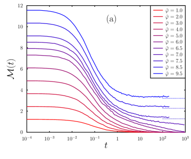
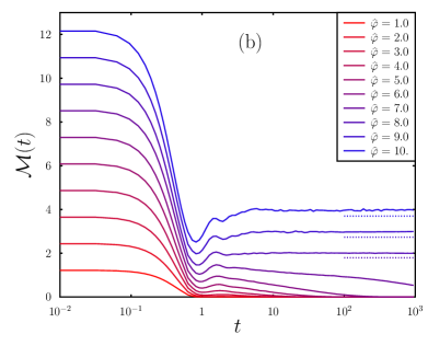
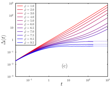
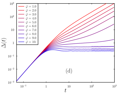
Figure 1: Numerical solution of the DMFT equations for the quadratic soft sphere potential at $\widehat{\varepsilon}=10$ and several densities $\widehat{\varphi}$. Top panels: memory kernels ${\cal M}(t)$ for Brownian (a) and Newtonian (b) dynamics. The memory functions in the liquid phase $\widehat{\varphi}<{\widehat{\varphi}}_{\rm d}\simeq 7.2458$ decays over a time scale that increases upon approaching the dynamical transition. In the dynamically arrested phase $\widehat{\varphi}>{\widehat{\varphi}}_{\rm d}$, a plateau emerges and ${\cal M}(t)\rightarrow{\cal M}_{\infty}>0$ for long times. The value of ${\cal M}_{\infty}(\widehat{\varphi})$ obtained from the plateau equation is plotted as a dashed lines with the same color as the corresponding density. Bottom panels: mean square displacement $\Delta(t)$ for Brownian (c) and Newtonian (d) dynamics. The long-time limit $\Delta_{\infty}=T^{2}/{\cal M}_{\infty}$ in the dynamically arrested phase is plotted as a dashed line.

V Results

In this section, we present results for ${\cal M}(t)$ and $\Delta(t)$ for soft and hard spheres, in both cases for Brownian and Newtonian dynamics. For soft spheres, we always use the quadratic potential, SQS with $\widehat{\varepsilon}=10$, unless otherwise specified. From the analysis of the plateau equations derived in section II.4, the dynamical glass transition happens at density $\widehat{\varphi}_{\rm d}\simeq 7.2458\ldots$ in this case. For hard spheres, the dynamical glass transition is at $\widehat{\varphi}^{\rm HS}_{\rm d}=4.8067\ldots$. Note that the dynamical glass transition line for SQS scales as $\widehat{\varphi}_{\rm d}-\widehat{\varphi}_{\rm d}^{\rm HS}\sim 6.13/\sqrt{\widehat{\varepsilon}}$ for $\widehat{\varepsilon}\rightarrow\infty$ Scalliet et al. (2019), which explains why the dynamical transition of SQS is quite distinct from that of hard spheres even at rather large $\widehat{\varepsilon}$.

V.1 Soft spheres

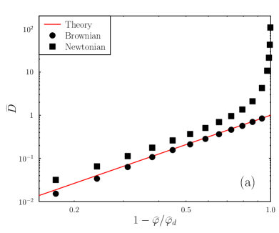
Figure 2: Numerical solution of the DMFT equations for the quadratic soft sphere potential at $\widehat{\varepsilon}=10$ and several densities $\widehat{\varphi}$. (a) Critical scaling of the diffusivity $\widehat{D}\sim(\widehat{\varphi}_{d}-\widehat{\varphi})^{\gamma}$ for $\widehat{\varphi}\rightarrow\widehat{\varphi}_{d}^{-}$, for Brownian (circles) and Newtonian (squares) dynamics. The line is the analytical prediction with ${\widehat{\varphi}}_{\rm d}=7.2458$ and $\gamma\simeq 2.25844$; the height of the line is adjusted to the plot. (b) Stokes-Einstein relation for Brownian and Newtonian dynamics, same key as left panel.

Results for ${\cal M}(t)$ obtained in Brownian and Newtonian dynamics are shown in Figs. 1a, 1b, respectively. The characteristic decay time of ${\cal M}(t)$ increases upon increasing density $\widehat{\varphi}$, corresponding to a dynamical slowing down, which becomes heavily pronounced for $\widehat{\varphi}=7.0$. For $\widehat{\varphi}\geq 7.50$, the memory exhibits a plateau as expected in the dynamically arrested phase. The numerical values of the memory can be compared to the analytical result for the plateau obtained from Eq. (13). The comparison is shown in Figs. 1a, 1b, with a fair agreement between analytical and numerical results. Note that while in the Brownian case ${\cal M}(t)$ is a monotonically decreasing function of $t$, in the Newtonian case we observe characteristic oscillations at intermediate times.

From the knowledge of ${\cal M}(t)$, the mean square displacement (MSD) can be easily computed through Eq. (3): the numerical results for the MSD versus time are shown in Figs. 1c, 1d. For $\widehat{\varphi}<{\widehat{\varphi}}_{\rm d}$, one finds the free particle behavior (diffusive for the Brownian and ballistic for the Newtonian dynamics) at short times and diffusive behavior at long times. Upon approaching the critical density ${\widehat{\varphi}}_{\rm d}$, the diffusion starts slowing down until the diffusion coefficient vanishes at ${\widehat{\varphi}}_{\rm d}$. A finite plateau, $\lim_{t\rightarrow\infty}\Delta(t)=\Delta_{\infty}$, is observed in the MSD at long times for $\widehat{\varphi}>{\widehat{\varphi}}_{\rm d}$. The long-time limit $\Delta_{\infty}$ can be compared to the asymptotic result from the plateau equation, which is given by $\Delta_{\infty}=T^{2}/{\cal M}_{\infty}$ from Eq. (3) Parisi et al. (2020).

We next discuss the critical behavior of the diffusivity upon approaching the dynamical transition. It is expected from the asymptotic analysis of the DMFT equations Kurchan et al. (2013); Parisi et al. (2020) that the diffusion coefficient $\widehat{D}$ defined in Eq. (4) follows a power-law behavior, i.e. $\widehat{D}\sim|{\widehat{\varphi}}_{\rm d}-\widehat{\varphi}|^{\gamma}$ when $\widehat{\varphi}\rightarrow{\widehat{\varphi}}_{\rm d}^{-}$, as in Mode Coupling Theory (MCT) Götze (2008). The critical exponent $\gamma$ can be computed for the SQS potential at $\widehat{\varepsilon}=10$, returning the value $\gamma\simeq 2.25844$ Kurchan et al. (2013); Parisi et al. (2020). The critical behavior is clearly seen in Fig. 2a. Interestingly, we find that in the Brownian case the power-law behavior is observed also for packing fractions rather distant from the critical point. On the other hand, the Newtonian diffusivity is diverging for low densities because of the ballistic motion in the absence of interactions. However, in both cases the agreement with the predicted critical scaling is very good; the difference in the prefactor is due to the difference in microscopic time units in Brownian and Newtonian dynamics. Note that for the points closest to ${\widehat{\varphi}}_{\rm d}$, the numerical estimate of ${\cal M}(t)$ at long times is less precise, which explains the slight deviation of the diffusivity from the expected power-law.

In the $d\rightarrow\infty$ limit, the diffusion coefficient and the viscosity are related by a generalized Stokes-Einstein relation Maimbourg et al. (2016); Charbonneau et al. (2018); Parisi et al. (2020). Indeed, the rescaled shear viscosity defined in Eq. (5) is given by the interaction term only when $d\rightarrow\infty$; therefore, Eqs. (4) and (5) lead to a slightly modified Stokes-Einstein relation (SER)

$$\beta\widehat{D}\widehat{\eta}_{s}=\frac{\beta\widehat{\varphi}\int_{0}^{\infty}\mathrm{d}t\,{\cal M}(t)}{\widehat{\zeta}+\beta\int_{0}^{\infty}\mathrm{d}t\,{\cal M}(t)}=\frac{\widehat{\varphi}}{1+\widehat{\zeta}\widehat{\varphi}/\widehat{\eta}_{s}}\ ,$$ (63)

which is plotted as a function of $\widehat{\varphi}$ in Fig. 2b. While this relation is trivial for the Newtonian case, in which $\beta\widehat{D}\widehat{\eta}_{s}=\widehat{\varphi}$ because $\widehat{\zeta}=0$, the same is not true for Brownian dynamics, in which the linear behavior is only recovered asymptotically close to the dynamical transition, where the viscosity diverges.

V.2 Brownian hard spheres

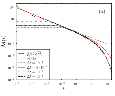
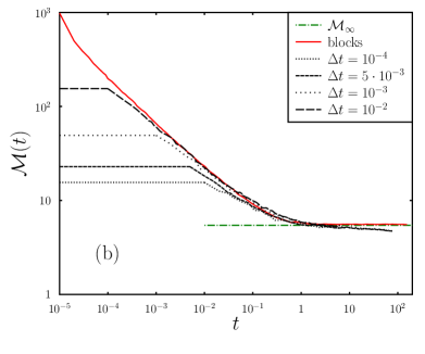
Figure 3: Numerical solution of the DMFT for Brownian hard spheres. Comparison between ${\cal M}(t)$ obtained on a fixed grid (black lines) and with a decimation algorithm (continuous red line), at $\widehat{\varphi}=$1.0 (a) and 7.0 (b). The simulations with fixed time grid are plotted for several time steps $\Delta t$. The decimation algorithm has $\Delta t_{\mathrm{min}}=10^{-5}$ and $\Delta t_{\mathrm{max}}=2\cdot 10^{-2}$. The dot-dashed green lines represent the short-time behavior from Eq. (24) (left), and the analytical plateau ${\cal M}_{\infty}$ at $\widehat{\varphi}=7.0$ (right) respectively.

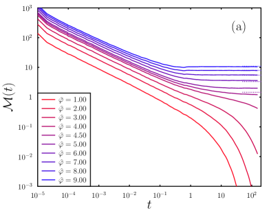
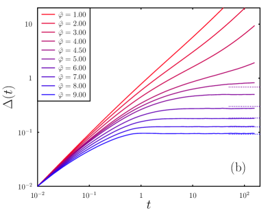
Figure 4: Numerical solution of the DMFT for Brownian hard spheres obtained via the decimation algorithm. (a) Memory function ${\cal M}(t)$ for several packing fractions given in the legend. Dashed lines correspond to the plateaus ${\cal M}_{\infty}$ when $\widehat{\varphi}>{\widehat{\varphi}}_{\rm d}\simeq 4.8067$. (b) Mean square displacement $\Delta(t)$ computed from the corresponding ${\cal M}(t)$, and comparison with the plateau $\Delta_{\infty}$.

The numerical results are less clear for Brownian hard spheres. In this case, we know from Eq. (24) that the short-time memory diverges as $t^{-1/2}$. We find that the numerical solution for ${\cal M}(t)$ depends on the discretization: in fact, the memory functions obtained through a fixed time grid and a decimation algorithm differ. The discrepancy is shown in Fig. 3, in which we show two cases with $\widehat{\varphi}=1.0$ and $\widehat{\varphi}=7.0$. Knowing that the critical density for hard spheres is ${\widehat{\varphi}}_{\rm d}\simeq 4.8067$, we expect to observe a complete decay in the dilute case and a plateau in the dense case. While the fixed-grid solutions approach the decimation solution for short times, there is a clear discrepancy at long times, which does not seem to depend on the time step $\Delta t$ chosen for the fixed-grid algorithm. Moreover, the fixed-grid solution at $\widehat{\varphi}=7.0$ slowly decays below the plateau, while the decimation algorithm solution is going to the expected plateau ${\cal M}_{\infty}\simeq 5.45227$ obtained from Eq. (52). While we do not have a clear explanation for this discrepancy, we suspect that the short-time cutoff to the square root divergence imposed by the fixed time step affects the memory function even at long times. The decimation algorithm is able to partially cure this problem because the short-time part of the memory function is integrated more accurately. The results obtained with the decimation algorithm are thus closer to the expected asymptotic limits.

The memory function ${\cal M}(t)$ obtained via the decimation algorithm is shown in Fig. 4, for $\widehat{\varphi}=1.0,2.0,\ldots,9.0$, and we observe a decay to zero in the liquid phase $\widehat{\varphi}<{\widehat{\varphi}}_{\rm d}$ and a plateau in the solid phase $\widehat{\varphi}>{\widehat{\varphi}}_{\rm d}$. However, the results display two main issues: first, there is a clear jump in the solution around $t\sim 1$ when we rescale $\Delta t\rightarrow 2\Delta t$, yielding an unphysical discontinuity in ${\cal M}(t)$. Second, the plateau is far from that obtained from Eq. (52) when $\widehat{\varphi}\rightarrow{\widehat{\varphi}}_{\rm d}^{+}$. The reason for these discrepancies is unclear, and we unfortunately must conclude that our numerical integration schemes are not reliable for Brownian hard spheres.

V.3 Newtonian hard spheres

The fixed time grid algorithm works well when considering Newtonian hard spheres. Indeed, in this case the memory kernel can be separated into a singular and a regular part, see Eq. (37). The singular part provides a white noise contribution in the dynamics in Eq. (43) which can be discretized in a standard way, so we only need to compute self-consistently the regular part ${\cal M}_{\rm reg}(t)$. We recall that a short-time exact analysis gives ${\cal M}_{\rm reg}(t)\sim 0.1578\,\widehat{\varphi}^{3}\,t$, see Appendix C.2. At long times, the memory function is expected to exhibit a plateau for $\widehat{\varphi}>{\widehat{\varphi}}_{\rm d}\simeq 4.8067$. These asymptotic results are well reproduced by the numerical solution, as it can be seen in Fig. 5a. The mean square displacements is shown in Fig. 5b. The scaling of the diffusivity is shown in Fig. 6a. The critical scaling $\widehat{D}\sim|\widehat{\varphi}_{d}-\widehat{\varphi}|^{\gamma}$ is confirmed, with the expected critical exponent $\gamma\simeq 2.33786$ Kurchan et al. (2013).

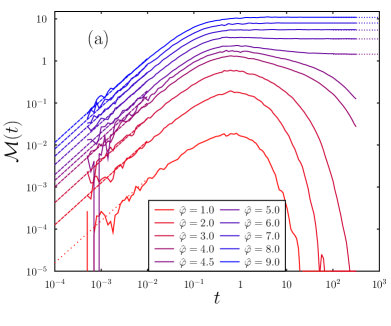
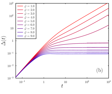
Figure 5: Numerical solution of the DMFT equations for Newtonian hard spheres. (a) Memory kernel ${\cal M}(t)$. The numerical solution (continuous lines) is compared to the short-time prediction ${\cal M}(t)\sim Ct$ with the constant $C$ obtained from Eq. (91) (dashed lines) and the expected plateau in the dynamically arrested phase (dotted lines). The curves are obtained by piecewise concatenation of the solution found with $\Delta t=10^{-4}$ up to $t_{\mathrm{max}}=1$ (short times) and the solution with $\Delta t=5\cdot 10^{-3}$ and $t_{\mathrm{max}}\sim 3\cdot 10^{2}$. (b) Mean square displacement computed from the numerical ${\cal M}(t)$. The dotted lines correspond to the static plateau $\Delta_{\infty}=T^{2}/{\cal M}_{\infty}$.

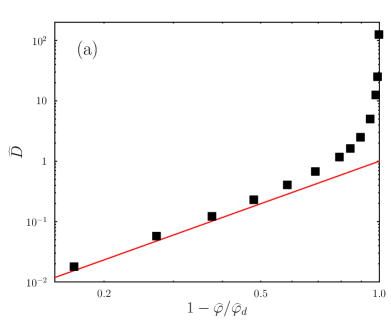
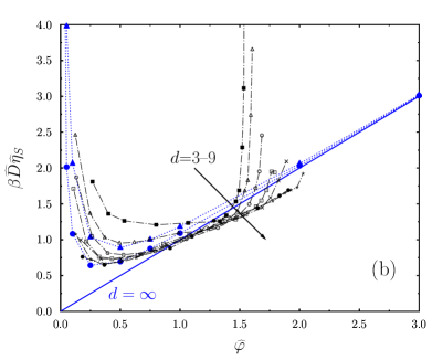
Figure 6: Numerical solution of the DMFT equations for Newtonian hard spheres. (a) Critical scaling of the diffusivity $\widehat{D}\sim({\widehat{\varphi}}_{\rm d}-\widehat{\varphi})^{\gamma}$ for $\widehat{\varphi}\rightarrow{\widehat{\varphi}}_{\rm d}^{-}$, as in Fig. 2a but with ${\widehat{\varphi}}_{\rm d}=4.8067$ and $\gamma=2.33786$. (b) Stokes-Einstein relation including the kinetic viscosity for Newtonian hard spheres, computed from Eq. (64) with $d=8$ and $d=12$ (blue points) and its $d=\infty$ limit (blue line). The black points correspond to MD simulations with $3\leq d\leq 9$, from Charbonneau et al. (2013).

In this paper we did not report any direct comparison between the $d\rightarrow\infty$ results and numerical data in finite $d$ because the latter are only available for $d\leq 10$ and finite $d$ corrections are usually too large to prevent a quantitative comparison with the $d\rightarrow\infty$ solution, except for the critical scaling around the dynamical glass transition Charbonneau et al. (2012, 2013). However, an exception is given by the Stokes-Einstein relation for Newtonian dynamics, for which the finite $d$ corrections seem unusually mild Charbonneau et al. (2013), which motivated us to attempt a systematic comparison with the solution of the DMFT equations. Note that in $d\rightarrow\infty$ the exact solution trivially gives $\beta\widehat{D}\widehat{\eta}_{s}=\widehat{\varphi}$ for any potential. However, the kinetic term provides a $1/d$ correction that diverges in the dilute regime, leading to

$$\beta\widehat{D}\widehat{\eta}_{s}=\widehat{\varphi}\left[1+\frac{1}{d}\frac{\int^{\infty}_{0}\mathrm{d}u\,\ddot{\Delta}(u)^{2}}{\int^{\infty}_{0}\mathrm{d}u\,{\cal M}(u)}\right]\ ,$$ (64)

where the integrals are computed on the dimensionless times $u=t/\tau_{N}$ and memory functions ${\cal M}(u)=\beta^{2}{\cal M}(u\cdot\tau_{N})$. The kinetic term vanishes in the $d\rightarrow\infty$ limit, but it also diverges in the dilute limit when $\widehat{\varphi}\rightarrow 0$ because the motion becomes ballistic at all times and the integral of $\ddot{\Delta}(t)^{2}$ diverges (see Appendix C.3). In Fig. 6b we plot our results from Eq. (64) together with finite-dimensional data from Ref. Charbonneau et al. (2013). The divergence of $\beta\widehat{D}\widehat{\eta}_{s}$ in the low-density regime is well visible, and the region over which it is observed shrinks upon increasing $d$, as expected. At finite value of $\widehat{\varphi}$, the results from Eq. (64) thus converge to the line $\beta\widehat{D}\widehat{\eta}_{s}=\widehat{\varphi}$ when $d\rightarrow\infty$. The finite-$d$ numerical data agree well with Eq. (64) in the low-density regime, while they seem to accumulate on a straight line with slope slightly smaller than one at higher density. We attribute this difference to the fact that $d$ is not large enough, so other subleading terms in $1/d$ could play a role. Note that the value of ${\widehat{\varphi}}_{\rm d}$ for $d=8$ is around ${\widehat{\varphi}}_{\rm d}\sim 2$, hence still quite distant from the asymptotic limit. In the vicinity of ${\widehat{\varphi}}_{\rm d}$, a steep increase of $\beta\widehat{D}\widehat{\eta}_{s}$ above the mean field prediction is observed. This “Stokes-Einstein relation breakdown” is a genuinely non-mean-field effect, related to dynamical heterogeneities Biroli and Bouchaud (2007); Berthier et al. (2011), and it vanishes in the limit $d\rightarrow\infty$ Charbonneau et al. (2013).

VI Conclusions

In this work, we analyzed the DMFT equations for infinite-dimensional equilibrium liquids derived in Maimbourg et al. (2016); Szamel (2017); Agoritsas et al. (2019a). We derived the DMFT equations for hard spheres as a limit of those for regular potentials, and we presented some methods to solve the DMFT equations numerically and analyze them analytically in some asymptotic limits. Our numerical solution algorithm is based on a straightforward discretization of time and an iterative calculation of the kernel ${\cal M}(t)$ via the self-consistent condition.

For soft spheres (both Brownian and Newtonian) and Newtonian hard spheres, we obtain accurate numerical solutions which agree well with the expected asymptotic limits (short times, long times, low density). The results confirm the presence of a dynamical glass transition with the same critical properties as Mode-Coupling Theory (although with different exponents), and provide the shape of the memory function and of the mean square displacement both in the liquid and glass phases. For Brownian hard spheres, the numerical integration scheme seems unable to properly handle the short-time divergence of the memory function, and the resulting numerical solutions are not fully consistent with the asymptotic limit. Better discretization schemes should then be developed, which is a non-trivial problem in stochastic calculus.

Unfortunately, the algorithm is limited to relatively short times, as it is often the case in the study of DMFT equations, which prevents us to investigate long-time phenomena such as the dynamic criticality around the glass transition (e.g. the stretching exponent of the memory function) and the aging dynamics in the glass phase Cugliandolo and Kurchan (1993); Cugliandolo (2003); Folena et al. (2019). A possible improvement would be the implementation of a decimation algorithm, which allows one to take exponentially growing time steps in the numerics and to observe the dynamics over several decades of time. Altough this method is well-established, e.g. in the numerical solution of Mode-Coupling Theory equations Fuchs et al. (1991); Liluashvili et al. (2017); Gruber et al. (2020), its extension to stochastic dynamics is missing. Such algorithm would represent a powerful tool for future investigations.

This work opens the way to the numerical solution of the DMFT equations in the non-equilibrium case Agoritsas et al. (2019a, b), which hopefully will give insight on a variety of phenomena such as yielding, jamming, and glass melting, both in passive and active systems. The simplest case is that of active matter in infinite dimensions de Pirey et al. (2019). While the approach of Ref. de Pirey et al. (2019) focuses on the stationary state distribution, DMFT also describes time-dependent correlations, as in the MCT approach of Refs. Berthier and Kurchan (2013); Szamel et al. (2015), and the approach to the stationary state itself. Work is currently in progress to solve, both analytically and numerically, the DMFT equations for the same model investigated in Ref. de Pirey et al. (2019). Another interesting case is that of rheology. Recently, MCT has been extended to describe the rheology of liquids and glasses, either in stationary state in the schematic limit Berthier et al. (2000), or via an integration-through-transient approach in the general setting Fuchs and Cates (2002); Brader et al. (2009, 2012). The same problem can be approached more phenomenologically via elastoplastic models Nicolas et al. (2018). It would be very interesting to compare DMFT with these complementary approaches.

Finally, a very important direction for future research is that of understanding the finite-$d$ corrections to DMFT in a systematic way. Ref. Baity-Jesi and Reichman (2019) reported a numerical calculation of ${\cal M}(t)$ in $d=3$, and a direct comparison with its DMFT approximation. This study should provide important insight on which terms have to be added to DMFT to obtain a more quantitative theory in finite $d$ Janssen and Reichman (2015); Charbonneau et al. (2018). Several groups are working in this direction to formulate a “cluster DMFT” Kotliar et al. (2001) of the glass transition. Another independent direction to tackle the same problem is that of looking for systematic deviations between DMFT and numerical results in high dimensions Biroli et al. (2020). This should allow one to identify the dominant corrections, such as hopping events (instantonic corrections) Charbonneau et al. (2014), facilitation effects Bhattacharyya et al. (2008), or fluctuations due to disorder Biroli and Bouchaud (2007); Sarlat et al. (2009); Franz et al. (2011); Rizzo and Voigtmann (2015, 2019).

Data availability statement

The data that support the findings of this study are available from the corresponding author upon reasonable request.

Appendix A Some details on Newtonian dynamics

We provide here some additional details on the formulation of the DMFT equations in the Newtonian case.

A.1 Distribution of the initial velocity

The distribution of the initial velocity $\dot{h}_{0}$ was not specified in Maimbourg et al. (2016); Agoritsas et al. (2019a, b) because it easily follows from the Maxwellian statistics of velocities in equilibrium. We provide some details here for completeness. Following (Agoritsas et al., 2019a, section 5.1), we define $y(t)=(d/\ell)\hat{\mathbf{r}}_{0}\cdot(\mathbf{u}_{1}(t)-\mathbf{u}_{2}(t))$, where $\hat{\mathbf{r}}_{0}$ is the unit vector along the initial distance between two particles (essentially a random unit vector by isotropy), and $\mathbf{u}_{1,2}$ are the displacements of the two particles with respect to their initial position at time $t=0$. According to the Maxwell distribution, each component of $\dot{\mathbf{u}}_{1,2}$ is an independent Gaussian variable with zero mean and variance $T/m$. As a consequence, $\dot{y}(t)$ is also a random Gaussian variable with zero mean and variance $(d^{2}/\ell^{2})2T/m=T/\widehat{m}$. Finally, $h(t)=h_{0}+y(t)+\Delta(t)$ and $\Delta(t)$ is ballistic at short times, hence $\dot{\Delta}(0)=0$, which implies that $\dot{h}_{0}=\dot{h}(0)=\dot{y}(0)$ is also a Gaussian variable with zero mean and standard deviation $T/\widehat{m}$. This justifies the probability distribution of $\dot{h}_{0}$ in Eq. (2).

A.2 Viscosity

The derivation of the viscosity in $d\rightarrow\infty$ is discussed in Maimbourg et al. (2016); Parisi et al. (2020) where, however, the kinetic term has been omitted. We provide here a more detailed discussion that is needed to compare with simulation results.

The shear viscosity is given in terms of the autocorrelation of the stress tensor in (Hansen and McDonald, 1986, Eq.(8.4.10)). The stress tensor, as given in (Hansen and McDonald, 1986, Eq.(8.4.14)), is the sum of a kinetic and an interaction terms. The contribution of the autocorrelation of the interaction term has been discussed in (Parisi et al., 2020, section 3.4.1), and is given by $\eta_{s}=\beta\rho d\int_{0}^{\infty}\mathrm{d}t\,{\cal M}(t)$. The other terms are subdominant when $d\rightarrow\infty$, but the autocorrelation of the kinetic term provides a divergent contribution for $\widehat{\varphi}\rightarrow 0$ that we need to add if we want to properly reproduce the ideal gas limit.

We are then going to neglect the cross-correlation of the kinetic and interaction terms, because it is subdominant both in $1/d\rightarrow 0$ and in $\widehat{\varphi}\rightarrow 0$, as deduced from  (Hansen and McDonald, 1986, Eq.(8.4.21)) and (Charbonneau et al., 2013, Eq.(D2)). The autocorrelation of the kinetic term can be written, neglecting velocity correlations between distinct particles in the limit $\widehat{\varphi}\rightarrow 0$, as

$$\eta_{\rm K}=\beta\rho m^{2}\int_{0}^{\infty}\mathrm{d}t\,Z(t)^{2}\ ,\qquad Z(t)=\left\langle v_{\mu}(t)v_{\mu}(0)\right\rangle=\frac{1}{2d}\frac{\mathrm{d}^{2}}{\mathrm{d}t^{2}}\left\langle|\mathbf{r}(t)-\mathbf{r}(0)|^{2}\right\rangle\ ,$$ (65)

where $Z(t)$ is the autocorrelation of a single spatial component of the velocity (Hansen and McDonald, 1986, Eq.(7.2.1)), related to the mean square displacement by (Hansen and McDonald, 1986, Eq.(7.2.5)) (here we considered a representative particle, without indicating explicitly the average over the $N$ particles). Recalling the scaling of mass and mean square displacement defined in section II.1, we obtain

$$\eta_{\rm K}=\beta\rho\widehat{m}^{2}\int_{0}^{\infty}\mathrm{d}t\,\ddot{\Delta}(t)^{2}\ .$$ (66)

Summing the kinetic and interaction contributions, we obtain Eq. (5).

Appendix B Brownian hard spheres

B.1 Backward Kolmogorov equation after the first iteration

We first provide some details on the backward Kolmogorov equation satisfied by the central quantity $G(h_{0},t)=\langle\theta(-h)\rangle_{h_{0}}$, i.e. the probability for a particle starting from $h_{0}$ to end up on the negative axis at time $t$. Here we consider the first iteration for the Brownian case, as studied in section III.1. By definition, this probability $G(h_{0},t)=\langle\theta(-h)\rangle_{h_{0}}$ can be computed by integrating the propagator $p_{\widehat{\varepsilon}}(h,t|h_{0})$ over the final position, i.e.,

$$G(h_{0},t)=\langle\theta(-h)\rangle_{h_{0}}=\int_{-\infty}^{0}\mathrm{d}h\,p_{\widehat{\varepsilon}}(h,t|h_{0})\;.$$ (67)

A natural way to compute $G(h_{0},t)$ would then be to write the standard (i.e. forward) Kolmogorov equation for the propagator $p_{\widehat{\varepsilon}}(h,t|h_{0})$, which, roughly speaking, amounts to study the dependence of $p_{\widehat{\varepsilon}}(h,t|h_{0})$ on the final position $h$. One would then solve this forward equation to obtain the propagator $p_{\widehat{\varepsilon}}(h,t|h_{0})$, insert this expression in (67) and integrate over the final position $h\in(-\infty,0)$ to get finally $G(h_{0},t)$. In such cases, there exists however a simpler way to do this computation, which avoids the explicit evaluation of the integral over the final position. It amounts to write instead the backward Kolmogorov equation for $p_{\widehat{\varepsilon}}(h,t|h_{0})$, which describes the dependence of $p_{\widehat{\varepsilon}}(h,t|h_{0})$ in the initial position $h_{0}$ (see e.g. Bray et al. (2013)). For a general Langevin equation as in (17) of the form

$$\dot{h}(t)=F[h(t)]+\Xi(t)\ ,\qquad\langle\Xi(t)\Xi(u)\rangle=2\,\delta(t-u)\ ,$$ (68)

for some force field $F[h(t)]$, it is well known that this backward Kolmogorov equation reads

$$\partial_{t}p_{\widehat{\varepsilon}}(h,t|h_{0})=\frac{\partial^{2}}{\partial h_{0}^{2}}p_{\widehat{\varepsilon}}(h,t|h_{0})+F[h_{0}]\frac{\partial}{\partial h_{0}}p_{\widehat{\varepsilon}}(h,t|h_{0})\;.$$ (69)

The interesting feature of this backward approach is that, by integrating this equation (69) over the final position $h\in(-\infty,0)$, one finds that $G(h_{0},t)$ in (67) actually satisfies exactly the same equation (69), namely

$$\partial_{t}G(h_{0},t)=\frac{\partial^{2}}{\partial h_{0}^{2}}G(h_{0},t)+F[h_{0}]\frac{\partial}{\partial h_{0}}G(h_{0},t)\;.$$ (70)

By specifying this equation (70) to the case $F[h_{0}]=1+\hat{\varepsilon}\theta(-h_{0})$, one obtains the equations given in (18). The initial and boundary conditions in (19) are then obtained by natural physical considerations.

B.2 Derivation of the Laplace transform of the first iteration

We provide here some details on the solution of Eq. (18) with boundary conditions in Eq. (19). Consider the Laplace transform $\widetilde{G}(h_{0},s)=\int_{0}^{\infty}\mathrm{d}te^{-st}G(h_{0},t)$. Using an integration by parts,

$$\int_{0}^{\infty}\mathrm{d}te^{-st}\dot{G}(h_{0},t)=s\widetilde{G}(h_{0},s)+[e^{-st}G(h_{0},t)]_{0}^{\infty}=s\widetilde{G}(h_{0},s)-G(h_{0},0)\ ,$$ (71)

and taking into account the first boundary condition in Eq. (19), we get

$$\begin{split}s\widetilde{G}(h_{0},s)-1&=\widetilde{G}^{\prime\prime}(h_{0},s)+(1+\widehat{\varepsilon})\widetilde{G}^{\prime}(h_{0},s)\ ,\qquad h_{0}<0\ ,\\ s\widetilde{G}(h_{0},s)&=\widetilde{G}^{\prime\prime}(h_{0},s)+\widetilde{G}^{\prime}(h_{0},s)\ ,\qquad\qquad\quad h_{0}>0\ .\end{split}$$ (72)

Taking into account the two other boundary conditions in Eq. (19), the solution is given by Eq. (20) with yet unknown functions $c_{\pm}(s)$. Now we should impose the continuity conditions in $h_{0}=0$. The leading singularity in Eq. (72) is of the form $\widetilde{G}^{\prime\prime}(h_{0},s)\approx\theta(h_{0})$ (note that a jump singularity comes from both the right and left hand sides of the equation), which implies that $\widetilde{G}(h_{0},s)$ and $\widetilde{G}^{\prime}(h_{0},s)$ are both continuous functions of $h_{0}$. This gives the conditions

$$\begin{split}\frac{1}{s}+c_{-}(s)&=c_{+}(s)\ ,\\ c_{-}(s)\lambda_{-}(s)&=c_{+}(s)\lambda_{+}(s)\ ,\end{split}$$ (73)

which imply

$$c_{-}(s)=\frac{\lambda_{+}(s)}{s[\lambda_{-}(s)-\lambda_{+}(s)]}\ ,\qquad c_{+}(s)=\frac{\lambda_{-}(s)}{s[\lambda_{-}(s)-\lambda_{+}(s)]}\ ,$$ (74)

thus completing the proof of Eq. (20).

B.3 Short-time behavior of the stress-stress correlation

The short-time behavior of the stress autocorrelation function $C_{\sigma\sigma}(t)=\beta\left\langle\Pi_{\mu\nu}(t)\Pi_{\mu\nu}(0)\right\rangle/V$ Hansen and McDonald (1986); Parisi et al. (2020) for Brownian hard spheres is given by kinetic theory for $d=3$ Lionberger and Russel (1994); Verberg et al. (1997); Lange et al. (2009), as

$$C_{\sigma\sigma}(t\rightarrow 0)=\frac{18}{5}\varphi^{2}g(\ell)\frac{\eta_{0}}{\tau}\sqrt{\frac{2\tau}{\pi t}}=\frac{24}{5\pi}\varphi^{2}g(\ell)\frac{T}{\ell^{3}}\sqrt{\frac{2\tau}{\pi t}}\ ,$$ (75)

where $\ell$ is the sphere diameter, $\varphi$ is the packing fraction, $g(\ell)$ is the contact value of the pair correlation function, $D_{0}=T/\zeta$ is the free particle diffusion coefficient, $\tau=\ell^{2}/(4D_{0})$, and $\eta_{0}$ is given by the Stokes expression $D_{0}=T/(3\pi\eta_{0}\ell)$.

According to Maimbourg et al. (2016); Parisi et al. (2020), when $d\rightarrow\infty$, the stress-stress autocorrelation is simply related to the memory function by

$$C_{\sigma\sigma}(t)=\beta\rho d{\cal M}(t)\ ,\qquad{\cal M}(t\rightarrow 0)\sim\frac{\widehat{\varphi}}{2}T^{2}\sqrt{\frac{\tau_{B}}{\pi t}}\qquad\Rightarrow\qquad C_{\sigma\sigma}(t\rightarrow 0)\sim\frac{2^{2d}\Gamma(1+d/2)}{2d\pi^{d/2}}\varphi^{2}\frac{T}{\ell^{d}}\sqrt{\frac{2\tau}{\pi t}}\ ,$$ (76)

where we used the short-time result for Brownian hard spheres reintroducing physical dimensions, with $\tau_{B}=\widehat{\zeta}/T=(\ell^{2}/2d^{2})\zeta/T=(\ell^{2}/2d^{2})/D_{0}=2\tau/d^{2}$, and $\rho=2^{d}\varphi/(V_{d}\ell^{d})$ with $V_{d}=\pi^{d/2}/\Gamma(1+d/2)$.

The two expressions in Eq. (75) and (76) match if we recall that $g(\ell)\rightarrow 1$ when $d\rightarrow\infty$ Parisi et al. (2020), and if we interpret the factor $5$ as $d+2$ in Eq. (75). This leads us to conjecture that in generic dimension $d$,

$$C_{\sigma\sigma}(t\rightarrow 0)\sim\frac{2^{2d}\Gamma(1+d/2)}{2(d+2)\pi^{d/2}}\varphi^{2}g(\ell)\frac{T}{\ell^{d}}\sqrt{\frac{2\tau}{\pi t}}\ ,$$ (77)

which coincides with Eq. (75) in $d=3$ and with Eq. (76) when $d\rightarrow\infty$, hence $d+2\approx d$. We were unable to find Eq. (77) in the literature, but it should follow from a straightforward generalization of the results of Refs. Lionberger and Russel (1994); Verberg et al. (1997); Lange et al. (2009) to arbitrary $d$.

B.4 Low-density limit of the diffusion coefficient

The calculation of the diffusion coefficient for Brownian hard spheres has been previously done for systems up to three dimensions Hanna et al. (1982); Ackerson and Fleishman (1982); Lekkerkerker and Dhont (1984). A first method consists in solving the Smoluchowski equation for the relative dynamics of two particles, and get the mean-square displacement and the diffusion coefficient from the calculation of the self-intermediate scattering function and the memory function; the second method requires to compute the mobility $\mu$ of a tagged particle under the action of a small force $\mathbf{F}$, and use the Einstein relation $D=T\mu$. Both methods agree that, when $d=2,3$, one finds at the first order in $\varphi$

$$D=D_{0}(1-2\varphi)\ ,$$ (78)

being $D_{0}$ the diffusion at $\varphi=0$ and $\varphi$ the packing fraction Lekkerkerker and Dhont (1984).

This second method can be extended to any dimension $d$: from (Lekkerkerker and Dhont, 1984, Eq. (17)), the pair distribution function $g(\mathbf{r})$ has the general form

$$g(\mathbf{r})=e^{-\beta v(r)}\left[1+\beta\ell\frac{Q(r)}{4r}\mathbf{r}\cdot\mathbf{F}\right]\ .$$ (79)

The radial function $Q(r)$ is determined by the differential equation in (Lekkerkerker and Dhont, 1984, Eq. (16)), which can be generalised to arbitrary dimension $d$ as

$$\frac{\mathrm{d}}{\mathrm{d}r}\left(e^{-\beta v(r)}r^{d-1}\frac{\mathrm{d}Q}{\mathrm{d}r}\right)-(d-1)r^{d-3}Q(r)e^{-\beta v(r)}+2\frac{r^{d-1}}{\ell}\frac{\mathrm{d}}{\mathrm{d}r}e^{-\beta v(r)}=0\ ,$$ (80)

with the boundary conditions $Q(r=\infty)=0$ and $Q^{\prime}(r=\ell)=-2/\ell$ for a hard sphere potential, leading to the general solution

$$Q(r)=\frac{2}{d-1}\left(\frac{\ell}{r}\right)^{d-1}\theta(r-\ell)\ .$$ (81)

The following result can be used to compute the force $\mathbf{F}_{\text{relax}}$ exerted on the tagged particle by the surrounding ones, given by (Lekkerkerker and Dhont, 1984, Eq. (24)), i.e.

$$\mathbf{F}_{\text{relax}}=\rho\int\mathrm{d}\mathbf{r}\,g(\mathbf{r})\,v^{\prime}(r)\frac{\mathbf{r}}{r}=-\frac{2^{d}}{2(d-1)}\varphi\,\mathbf{F}\ .$$ (82)

The total force acting on the tagged particle is therefore $\mathbf{F}_{\text{total}}=\mathbf{F}+\mathbf{F}_{\text{relax}}=[1-2^{d}\varphi/(2(d-1))]\mathbf{F}$. The coefficient of $\mathbf{F}$ coincides with the low-density correction to the mobility $\mu$ and the diffusion coefficient then reads

$$D=D_{0}\left(1-\frac{2^{d}}{2(d-1)}\varphi\right)=\begin{cases}D_{0}\left(1-2\varphi\right)&d=2,\,3\\[5.69046pt] D_{0}\left(1-\frac{1}{2}\widehat{\varphi}\right)&d\rightarrow\infty\end{cases}\ ,$$ (83)

recalling that $\widehat{\varphi}=2^{d}\varphi/d$. This result generalizes the low-density correction obtained for $d=2,3$ and extends it towards the infinite-dimensional limit, consistently with the DMFT result given in Eq. (23).

Appendix C Newtonian hard spheres

C.1 Short-time expansion from kinetic theory

In infinite dimensions, the memory function is related to the velocity autocorrelation Baity-Jesi and Reichman (2019). We follow the notations of Parisi et al. (2020) and denote the non-scaled mean square displacement by $\operatorname{\mathsf{D}}(t)=\left\langle|\mathbf{r}(t)-\mathbf{r}(0)|^{2}\right\rangle$. According to Eq. (65), the velocity autocorrelation is $Z(t)=\ddot{\operatorname{\mathsf{D}}}(t)/(2d)$ Hansen and McDonald (1986). In the infinite dimensional limit, for Newtonian dynamics, the non-scaled memory function $M(t)=(2d^{2}/\ell^{2}){\cal M}(t)$ is related to $\operatorname{\mathsf{D}}(t)$ by Parisi et al. (2020)

$$m\ddot{\operatorname{\mathsf{D}}}(t)=2dT-\beta\int_{0}^{t}\mathrm{d}uM(t-u)\dot{\operatorname{\mathsf{D}}}(u)\ ,$$ (84)

which in Laplace space, using $s^{2}\widetilde{\operatorname{\mathsf{D}}}(s)=2d\widetilde{Z}(s)$, reads

$$m\widetilde{Z}(s)=T/s-\beta\widetilde{M}(s)\widetilde{Z}(s)/s\qquad\Rightarrow\qquad\widetilde{M}(s)=\frac{T-ms\widetilde{Z}(s)}{\beta\widetilde{Z}(s)}\ .$$ (85)

Kinetic theory De Schepper et al. (1981); Bishop et al. (1985); Leegwater and van Beijeren (1989); Dufty and Ernst (2004) gives the short-time expansion of $Z(t)$ in arbitrary dimension as

$$\frac{Z(t)}{Z(0)}=1-\frac{2|t|}{d\,\tau_{E}}+A_{d}\left(\frac{t}{\tau_{E}}\right)^{2}+{\cal O}(t^{3})\ ,\qquad\tau_{E}=\frac{\sqrt{\pi\beta m}}{d\,2^{d}\varphi}\frac{\ell}{g(\ell)}\ ,\qquad A_{d}=\frac{2}{d^{2}}{}_{2}F_{1}\left(-\frac{1}{2},-\frac{1}{2};\frac{1}{2}(d+2);\frac{1}{4}\right)\ ,$$ (86)

where $Z(0)=T/m$. Moving to Laplace space and plugging this expansion in Eq. (85) we get

$$\widetilde{M}(s)=\frac{2Tm}{d\,\tau_{E}}\left[1+\frac{2(1-A_{d})}{d\,\tau_{E}}\frac{1}{s}+{\cal O}\left(\frac{1}{s^{2}}\right)\right]\ .$$ (87)

This result shows that $M(t)$ is indeed the sum of a delta function and a regular function, which admits a short time expansion in integer powers of $t$. Taking the $d\rightarrow\infty$ limit with the rescaling $\widehat{m}=(\ell^{2}/2d^{2})m$, $2^{d}\varphi=d\widehat{\varphi}$, ${\cal M}(t)=(\ell^{2}/2d^{2})M(t)$, and using $g(\ell)\rightarrow 1$ and $A_{d}=1+\alpha/d+\cdots$, we obtain

$$\widetilde{\cal M}(s)=\widehat{\varphi}\sqrt{\frac{2T\widehat{m}}{\pi}}\left[1-\frac{2\alpha}{d\,\tau}\frac{1}{s}+{\cal O}\left(\frac{1}{s^{2}}\right)\right]\ ,\qquad\tau=d\,\tau_{E}=\frac{\sqrt{2\pi\beta\widehat{m}}}{\widehat{\varphi}}\ .$$ (88)

This result proves Eq. (36) when transformed back to the time domain. In particular, the coefficient of the delta peak coincides with the result obtained from DMFT, and the value of ${\cal M}_{\rm reg}(t=0)$ is found to vanish proportionally to $1/d$ for $d\rightarrow\infty$. Unfortunately, to our knowledge the next term of the short-time expansion has not been computed in finite $d$.

C.2 Short-time expansion of the regular part of the memory function within DMFT

The regular part of the memory function ${\cal M}_{\text{reg}}(t)$ for Newtonian hard spheres can be analytically computed for short times. Keeping only the leading short-time singularity ${\cal M}(t)=2\zeta_{0}\delta(t)$ as given in Eq. (34), the evolution of $h(t)$ reads

$$\begin{split}\ddot{h}(t)+\zeta_{0}\dot{h}(t)&=1+\Xi(t)\ ,\quad h(t)>0\\ h(t=0)&=0\ ,\quad\dot{h}(t=0)=g_{0}\ ,\\ \langle\Xi(t)\Xi(u)\rangle&=2\zeta_{0}\delta(t-u)\ .\end{split}$$ (89)

Because this white noise dominates at short times, we expect that in order to obtain the short-time behavior of ${\cal M}_{\text{reg}}(t)$ we can neglect the regular part in the stochastic process, i.e. we use the process in Eq. (89). Furthermore, at short times we can approximate the return probability by the first return probability, i.e. neglect multiple returns. The computation of the first return probability density $f(g_{1},t|g_{0})$ defined in Eq. (45) is a Wang-Uhlenbeck recurrence time problem. Note that in the absence of the term $\zeta_{0}\dot{h}(t)$, Eq. (89) reduces to the random acceleration process in the presence of a linear drift Burkhardt (2007), for which the first passage time distribution can be computed exactly Burkhardt (2008). In presence of the linear drift, the problem can be solved analytically for short times. In our units, we obtain Singer and Schuss (2005) (see also McKean (1962); Burkhardt (2008))

$$f(g_{1},t|g_{0})\sim\frac{\sqrt{3}\,|g_{1}|}{2\pi\zeta_{0}t^{2}}\exp\left(\frac{g^{2}_{0}-g^{2}_{1}}{4}-\frac{g_{0}-g_{1}}{2\zeta_{0}}-\frac{g_{1}^{2}+g_{1}g_{0}+g_{0}^{2}}{\zeta_{0}t}\right)\text{erf}\left(\sqrt{\frac{3|g_{1}|g_{0}}{\zeta_{0}t}}\right).$$ (90)

The latter result can be plugged into Eq. (48), and the integral can be performed with the change of variables $u_{i}=|g_{i}|/\sqrt{\zeta_{0}t}$ for $i=0,1$ and expanding around $t=0$. Setting now $\zeta_{0}=\sqrt{2/\pi}\widehat{\varphi}$, one finds

$${\cal M}_{\text{reg}}(t)\sim\frac{\sqrt{6}}{\pi^{5/2}}\left[\int^{\infty}_{0}\mathrm{d}u_{0}\int_{0}^{\infty}\mathrm{d}u_{1}u_{0}^{2}\,u_{1}^{2}\,e^{-(u_{1}^{2}-u_{0}u_{1}+u_{0}^{2})}\,\text{erf}\left(\sqrt{3u_{1}u_{0}}\right)\right]\,\widehat{\varphi}^{3}\,t=C_{0}\,\widehat{\varphi}^{3}\,t\ ,$$ (91)

with $C_{0}\simeq 0.1578$. This result confirms that $B=0$ and $C=C_{0}\,\widehat{\varphi}^{3}$ when $d=\infty$ in Eq. (36). This short-time behavior has been plotted in Fig. 5a, showing a good agreement with the numerical solution of DMFT.

C.3 Low-density regime of the DMFT equations

When $\widehat{\varphi}\ll 1$, the regular part of the memory function is negligible, therefore ${\cal M}(t)=2\zeta_{0}\,\delta(t)$. Using Eq. (3) in dimensionless units, with the above-mentioned memory kernel and $\widehat{\zeta}=0$ one finds the solution

$$\Delta(t)=\frac{1}{\zeta_{0}}\left[t-\frac{1}{\zeta_{0}}\left(1-e^{-\zeta_{0}\,t}\right)\right]\ ,$$ (92)

corresponding to the characteristic MSD of underdamped, dilute dynamics, with a ballistic regime for $t\ll\zeta_{0}^{-1}$ and a diffusive regime for $t\gg\zeta_{0}^{-1}$. This allows one to compute analytically the viscosity and diffusion constant. The two integrals in Eq. (64) can be explicitly computed and give $\int_{0}^{\infty}\mathrm{d}u\,\ddot{\Delta}(u)^{2}=(2\zeta_{0})^{-1}$ and $\int_{0}^{\infty}\mathrm{d}u\,{\cal M}(u)=\zeta_{0}$. Recalling that $\zeta_{0}=\sqrt{2/\pi}\,\widehat{\varphi}$, one finds

$$\beta\widehat{D}\widehat{\eta}_{s}=\widehat{\varphi}\left(1+\frac{\pi}{4d\widehat{\varphi}^{2}}\right)\ ,$$ (93)

leading to the dilute-limit divergence $\beta\widehat{D}\widehat{\eta}_{s}\approx\pi/(4d\,\widehat{\varphi})$ when $\widehat{\varphi}\rightarrow 0$ in any finite dimension. This divergence disappears when $d\rightarrow\infty$.

References

- Hansen and McDonald (1986) J.-P. Hansen and I. R. McDonald, Theory of simple liquids (Third edition) (Academic Press, 1986).
- Bengtzelius et al. (1984) U. Bengtzelius, W. Götze, and A. Sjolander, Journal of Physics C: Solid State Physics 17, 5915 (1984).
- Götze (2008) W. Götze, Complex dynamics of glass-forming liquids: a mode-coupling theory (Oxford University Press, 2008).
- Das and Mazenko (1986) S. P. Das and G. F. Mazenko, Physical Review A 34, 2265 (1986).
- Andreanov et al. (2006) A. Andreanov, G. Biroli, and A. Lefèvre, Journal of Statistical Mechanics: Theory and Experiment 2006, P07008 (2006).
- Kim and Kawasaki (2007) B. Kim and K. Kawasaki, Journal of Physics A: Mathematical and Theoretical 40, F33 (2007).
- Jacquin and Van Wijland (2011) H. Jacquin and F. Van Wijland, Physical Review Letters 106, 210602 (2011).
- Götze (1999) W. Götze, Journal of Physics: Condensed Matter 11, A1 (1999).
- Frisch et al. (1985) H. L. Frisch, N. Rivier, and D. Wyler, Physical Review Letters 54, 2061 (1985).
- Frisch and Percus (1987) H. Frisch and J. Percus, Physical Review A 35, 4696 (1987).
- Wyler et al. (1987) D. Wyler, N. Rivier, and H. L. Frisch, Physical Review A 36, 2422 (1987).
- Frisch and Percus (1999) H. L. Frisch and J. K. Percus, Physical Review E 60, 2942 (1999).
- Kirkpatrick and Wolynes (1987) T. R. Kirkpatrick and P. G. Wolynes, Physical Review A 35, 3072 (1987).
- Elskens and Frisch (1988) Y. Elskens and H. L. Frisch, Physical Review A 37, 4351 (1988).
- Maimbourg et al. (2016) T. Maimbourg, J. Kurchan, and F. Zamponi, Physical Review Letters 116, 015902 (2016).
- Szamel (2017) G. Szamel, Physical Review Letters 119, 155502 (2017).
- Agoritsas et al. (2018) E. Agoritsas, G. Biroli, P. Urbani, and F. Zamponi, Journal of Physics A: Mathematical and Theoretical 51, 085002 (2018).
- Agoritsas et al. (2019a) E. Agoritsas, T. Maimbourg, and F. Zamponi, Journal of Physics A: Mathematical and Theoretical 52, 144002 (2019a).
- Georges et al. (1996) A. Georges, G. Kotliar, W. Krauth, and M. J. Rozenberg, Reviews of Modern Physics 68, 13 (1996).
- Charbonneau et al. (2017) P. Charbonneau, J. Kurchan, G. Parisi, P. Urbani, and F. Zamponi, Ann. Rev. of Cond. Matter Physics 8, 265 (2017).
- Agoritsas et al. (2019b) E. Agoritsas, T. Maimbourg, and F. Zamponi, Journal of Physics A: Mathematical and Theoretical 52, 334001 (2019b).
- Parisi et al. (2020) G. Parisi, P. Urbani, and F. Zamponi, Theory of Simple Glasses: Exact Solutions in Infinite Dimensions (Cambridge University Press, 2020).
- de Pirey et al. (2019) T. A. de Pirey, G. Lozano, and F. van Wijland, Physical Review Letters 123, 260602 (2019).
- Cugliandolo (2003) L. F. Cugliandolo, in Slow relaxations and nonequilibrium dynamics in condensed matter, edited by J. Barrat, M. Feigelman, J. Kurchan, and J. Dalibard (Springer-Verlag, 2003), eprint arXiv.org:cond-mat/0210312.
- Bray et al. (2013) A. J. Bray, S. N. Majumdar, and G. Schehr, Advances in Physics 62, 225 (2013).
- Lionberger and Russel (1994) R. A. Lionberger and W. B. Russel, Journal of Rheology 38, 1885 (1994).
- Verberg et al. (1997) R. Verberg, I. M. De Schepper, M. J. Feigenbaum, and E. G. D. Cohen, Journal of Statistical Physics 87, 1037 (1997).
- Lange et al. (2009) E. Lange, J. B. Caballero, A. M. Puertas, and M. Fuchs, The Journal of Chemical Physics 130, 174903 (2009).
- Hanna et al. (1982) S. Hanna, W. Hess, and R. Klein, Physica A: Statistical Mechanics and its Applications 111, 181 (1982).
- Ackerson and Fleishman (1982) B. J. Ackerson and L. Fleishman, The Journal of Chemical Physics 76, 2675 (1982).
- Lekkerkerker and Dhont (1984) H. Lekkerkerker and J. Dhont, The Journal of chemical physics 80, 5790 (1984).
- Alder and Wainwright (1970) B. Alder and T. Wainwright, Physical review A 1, 18 (1970).
- Borodin and Salminen (2012) A. N. Borodin and P. Salminen, Handbook of Brownian motion - facts and formulae (Birkhäuser, 2012).
- Dufty (2002) J. W. Dufty, Molecular Physics 100, 2331 (2002).
- Brańka and Heyes (2004) A. Brańka and D. M. Heyes, Physical Review E 69, 021202 (2004).
- De Schepper et al. (1981) I. M. De Schepper, M. H. Ernst, and E. G. D. Cohen, Journal of Statistical Physics 25, 321 (1981).
- Bishop et al. (1985) M. Bishop, J. Michels, and I. De Schepper, Physics Letters A 111, 169 (1985).
- Miyazaki et al. (2001) K. Miyazaki, G. Srinivas, and B. Bagchi, The Journal of Chemical Physics 114, 6276 (2001).
- Charbonneau et al. (2013) B. Charbonneau, P. Charbonneau, Y. Jin, G. Parisi, and F. Zamponi, Journal of Chemical Physics 139, 164502 (2013).
- Singer and Schuss (2005) A. Singer and Z. Schuss, Physical Review Letters 95, 110601 (2005).
- Burkhardt (2007) T. W. Burkhardt, Journal of Statistical Mechanics: Theory and Experiment 2007, P07004 (2007).
- Roy et al. (2019) F. Roy, G. Biroli, G. Bunin, and C. Cammarota, Journal of Physics A: Mathematical and Theoretical 52, 484001 (2019).
- Kim and Latz (2001) B. Kim and A. Latz, EPL (Europhysics Letters) 53, 660 (2001).
- Scalliet et al. (2019) C. Scalliet, L. Berthier, and F. Zamponi, Physical Review E 99, 012107 (2019).
- Kurchan et al. (2013) J. Kurchan, G. Parisi, P. Urbani, and F. Zamponi, The Journal of Physical Chemistry B 117, 12979 (2013).
- Charbonneau et al. (2018) B. Charbonneau, P. Charbonneau, and G. Szamel, The Journal of Chemical Physics 148, 224503 (2018).
- Charbonneau et al. (2012) P. Charbonneau, E. I. Corwin, G. Parisi, and F. Zamponi, Physical Review Letters 109, 205501 (2012).
- Biroli and Bouchaud (2007) G. Biroli and J. Bouchaud, J. Phys.: Cond. Matt. 19, 205101 (2007).
- Berthier et al. (2011) L. Berthier, G. Biroli, J.-P. Bouchaud, L. Cipelletti, and W. van Saarloos, Dynamical heterogeneities and glasses (Oxford University Press, 2011).
- Cugliandolo and Kurchan (1993) L. F. Cugliandolo and J. Kurchan, Physical Review Letters 71, 173 (1993).
- Folena et al. (2019) G. Folena, S. Franz, and F. Ricci-Tersenghi, arXiv:1903.01421 (2019).
- Fuchs et al. (1991) M. Fuchs, W. Götze, I. Hofacker, and A. Latz, Journal of Physics: Condensed Matter 3, 5047 (1991).
- Liluashvili et al. (2017) A. Liluashvili, J. Ónody, and T. Voigtmann, Phys. Rev. E 96, 062608 (2017).
- Gruber et al. (2020) M. Gruber, A. M. Puertas, and M. Fuchs, Phys. Rev. E 101, 012612 (2020).
- Berthier and Kurchan (2013) L. Berthier and J. Kurchan, Nature Physics 9, 310 (2013).
- Szamel et al. (2015) G. Szamel, E. Flenner, and L. Berthier, Phys. Rev. E 91, 062304 (2015).
- Berthier et al. (2000) L. Berthier, J.-L. Barrat, and J. Kurchan, Physical Review E 61, 5464 (2000).
- Fuchs and Cates (2002) M. Fuchs and M. E. Cates, Physical Review Letters 89, 248304 (2002).
- Brader et al. (2009) J. M. Brader, T. Voigtmann, M. Fuchs, R. G. Larson, and M. E. Cates, Proceedings of the National Academy of Sciences 106, 15186 (2009).
- Brader et al. (2012) J. M. Brader, M. E. Cates, and M. Fuchs, Physical Review E 86, 021403 (2012).
- Nicolas et al. (2018) A. Nicolas, E. E. Ferrero, K. Martens, and J.-L. Barrat, Reviews of Modern Physics 90, 045006 (2018).
- Baity-Jesi and Reichman (2019) M. Baity-Jesi and D. R. Reichman, The Journal of Chemical Physics 151, 084503 (2019).
- Janssen and Reichman (2015) L. M. C. Janssen and D. R. Reichman, Physical Review Letters 115, 205701 (2015).
- Kotliar et al. (2001) G. Kotliar, S. Y. Savrasov, G. Pálsson, and G. Biroli, Physical review letters 87, 186401 (2001).
- Biroli et al. (2020) G. Biroli, P. Charbonneau, E. I. Corwin, Y. Hu, H. Ikeda, G. Szamel, and F. Zamponi, arXiv:2003.11179 (2020).
- Charbonneau et al. (2014) P. Charbonneau, Y. Jin, G. Parisi, and F. Zamponi, Proceedings of the National Academy of Sciences 111, 15025 (2014).
- Bhattacharyya et al. (2008) S. M. Bhattacharyya, B. Bagchi, and P. G. Wolynes, Proceedings of the National Academy of Sciences 105, 16077 (2008).
- Sarlat et al. (2009) T. Sarlat, A. Billoire, G. Biroli, and J.-P. Bouchaud, Journal of Statistical Mechanics: Theory and Experiment 2009, P08014 (2009).
- Franz et al. (2011) S. Franz, G. Parisi, F. Ricci-Tersenghi, and T. Rizzo, The European Physical Journal E 34, 1 (2011).
- Rizzo and Voigtmann (2015) T. Rizzo and T. Voigtmann, Europhysics Letters 111, 56008 (2015).
- Rizzo and Voigtmann (2019) T. Rizzo and T. Voigtmann, arXiv:1903.01773 (2019).
- Leegwater and van Beijeren (1989) J. A. Leegwater and H. van Beijeren, Journal of Statistical Physics 57, 595 (1989).
- Dufty and Ernst (2004) J. W. Dufty and M. H. Ernst, Molecular Physics 102, 2123 (2004).
- Burkhardt (2008) T. W. Burkhardt, Journal of Statistical Physics 133, 217 (2008).
- McKean (1962) H. P. McKean, Journal of mathematics of Kyoto University 2, 227 (1962).