cutpointr: Improved Estimation and Validation of Optimal Cutpoints in R

Christian Thiele, Gerrit Hirschfeld cutpointr: Improved estimation and validation of optimal cutpoints in R cutpointr: Improved Estimation and Validation of Optimal Cutpoints in R “Optimal cutpoints” for binary classification tasks are often established by testing which cutpoint yields the best discrimination, for example the Youden index, in a specific sample. This results in “optimal” cutpoints that are highly variable and systematically overestimate the out-of-sample performance. To address these concerns, the cutpointr package offers robust methods for estimating optimal cutpoints and the out-of-sample performance. The robust methods include bootstrapping and smoothing based on kernel estimation, generalized additive models, smoothing splines, and local regression. These methods can be applied to a wide range of binary-classification and cost-based metrics. cutpointr also provides mechanisms to utilize user-defined metrics and estimation methods. The package has capabilities for parallelization of the bootstrapping, including reproducible random number generation. Furthermore, it is pipe-friendly, for example for compatibility with functions from tidyverse. Various functions for plotting receiver operating characteristic curves, precision recall graphs, bootstrap results and other representations of the data are included. The package contains example data from a study on psychological characteristics and suicide attempts suitable for applying binary classification algorithms. optimal cutpoint, ROC curve, bootstrap, R optimal cutpoint, ROC curve, bootstrap, R Christian Thiele
University of Applied Sciences Bielefeld
Interaktion 1 33619 Bielefeld, Germany
E-mail:
URL: http://www.fh-bielefeld.de
 

1 Introduction

In many applied fields “optimal cutpoints” are used to aid the interpretation of continuous test results or measurements. In medicine, optimal cutpoints are used to determine the level of a laboratory marker at which specific interventions should be triggered. In psychology, optimal cutpoints are used to screen for disorders, for example for depression or suicidality. Given the importance of cutpoints, a lot of research is focused on empirically determining “optimal cutpoints”. Usually, applied researchers collect data both on the continuous measure for which a cutpoint is being developed and on a reference test (gold standard). An optimal cutpoint is then determined by computing a measure of discriminative ability at all cutpoints and choosing the cutpoint as “optimal” that optimizes this measure in the sample.

Unfortunately, cutpoints that are determined this way are highly sample-specific and overestimate the diagnostic utility of the measure. Altman et al. observed more than twenty years ago that different studies which empirically determined optimal cutpoints for prognostic markers in breast cancer (Altman et al., 1994) yield highly conflicting optimal cutpoints. Furthermore, the post-hoc choice of optimal cutpoints introduces a positive bias to the estimated discriminative ability (Ewald, 2006; Hirschfeld and do Brasil, 2014). To overcome the former problem, more robust methods to estimate optimal cutpoints have been developed (Fluss et al., 2005; Leeflang et al., 2008). In parallel, methods to estimate the out-of-sample performance of predictive models have been developed but have not been applied to the estimation of cutpoint performance. cutpointr is an R (R Core Team, 2018) package that was developed to make robust estimation procedures for optimal cutpoints and their out-of-sample performance more accessible (see Section 2 and Section 3). It is available from the Comprehensive R Archive Network (CRAN) at https://cran.r-project.org/package=cutpointr.

Furthermore, cutpointr was developed with three design goals in mind. First, to make computationally demanding methods such as bootstrapping feasible, we wanted to improve the performance and scalability of optimal cutpoint procedures. With larger data (say, more than 1 million observations) some of the existing solutions and packages are prohibitively slow or not memory-efficient enough. The cutpointr package aims at better performance with larger data. The included bootstrapping routine can easily be run in parallel by setting the allowParallel parameter to TRUE and registering a parallel backend before running cutpointr. Second, for convenient integration into workflows that employ functions from the “tidyverse” cutpointr is pipe-friendly by making data the first argument and providing the output as a data frame which can be easily piped to further functions. The output is tidy (Wickham et al., 2014) in the sense that every column represents a variable and every observation is a row. It may on the other hand be untidy in the sense that it contains some columns that are observations on the level of the model or data set and thus constant over subgroups (e.g., AUC), if subgroups are specified. The original data, the receiver operating characteristic (ROC) curve and, if desired, the results of the bootstrapping are returned in nested tibbles. Third, cutpointr tries to offer an intuitive interface. For example, it allows for control over the positive and negative classes as well as the direction that defines whether higher or lower values of the predictor stand for the positive class. If these are left out, cutpointr will attempt to determine these parameters automatically and use sensible defaults. The package should be applicable in a wide variety of tasks and tries to avoid focusing on a specific field of study, for example by a wording of the documentation and function arguments that is as general as possible.

At present, several other packages for the R environment for statistical computing and graphics exist that calculate optimal cutpoints or ROC curves. Most notably, OptimalCutpoints (López-Ratón et al., 2014) was specifically designed to calculate cutpoints. While this package implements a wide range of metrics for diagnostic utility, it lacks the ability for robust cutpoint estimation and out-of-sample validation. Additionally, GsymPoint (López-Ratón et al., 2017) provides alternative estimation procedures for the generalized symmetry point and ThresholdROC (Perez-Jaume et al., 2017) offers several optimization methods for application on two- and three-class problems. ROCR (Sing et al., 2005), that was developed for ROC curve analysis, can also be used to calculate optimal cutpoints after writing short functions that search for the optimal metric value and return the corresponding cutpoint. pROC (Robin et al., 2011) offers cutpoint estimation in terms of two metrics including weighting of false positives and false negatives. Most of these packages do not offer functions that perform robust estimation of optimal cutpoints or provide procedures to assess the variability and out-of-sample performance of the optimal cutpoints.

Furthermore, the packages differ widely in their choice of and control over the specifics of the cutpoint calculation, such as the direction and the use of midpoints (table 1). Only some packages offer the choice of the direction, that is whether higher or lower values of the predictor stand for the positive or negative class, or in other words the direction of the ROC curve. Some packages allow for the automatic detection of a plausible direction. All of the packages except for cutpointr make the choice of whether or not to use midpoints implicitly. These seemingly minute choices become relevant when small datasets are analyzed (simulation results can be found in the package vignette, see vignette("cutpointr")). cutpointr supports either choosing the direction of the ROC curve manually or detecting it automatically. Whether or not midpoints are returned can be specified.

	Cutpoint	Robust	Direction			Returns
Package	optimization	cutpoints	Settings	Behavior	Automatic	midpoints
					available
cutpointr	yes	yes	>=	>=	yes	selectable
			<=	<=
OptimalCutpoints	yes	no	>	>	no	no
			<	<
pROC	yes	no	>	>	yes	yes
			<	<
ROCR	no	no	none	>	no	no
ThresholdROC	yes	yes	none	>=	yes	no
				<=

Table 1: Features, settings and actual behavior regarding direction and midpoints of relevant packages for ROC curve analysis or cutpoint optimization.

The rest of the article is structured as follows. In section 2 we describe the different methods to determine optimal cutpoints, focusing on both the metrics used to determine cutpoints, for example the Youden index or cost based methods, as well as the methods to select a cutpoint, for example LOESS-based smoothing or bootstrapping. In section 3 we describe the bootstrapping method to estimate the out-of sample performance and the variability of the cutpoints. In section 4 we compare the performance of different estimation methods on simulated data. In section 5 we show how these methods are implemented in cutpointr. In section 6 we show how these can be used to analyze an example dataset on optimal cutpoints for suicide. In section 7 we offer some concluding remarks.

2 Estimating optimal cutpoints

Optimal cutpoints are estimated by choosing a specific metric that is being used to quantify the discriminatory ability and a specific method to select a cutpoint as optimal based on this metric. The most widely-used combination of these two is to use the Youden index as a metric and to select the cutpoint as optimal that empirically maximizes the Youden index in-sample. In the following, we discuss several alternative metrics and methods. While the choice of metrics has received ample attention, the methods to determine optimal cutpoints have been largely neglected.

2.1 Metrics to quantify discriminatory ability

Most of the metrics to assess the discriminatory ability of a cutpoint rely on the elements of the $2\times 2$ confusion matrix, that is true positives ($TP$), false positives ($FP$), true negatives ($TN$), and false negatives ($FN$). Sensitivity is defined as ($TP$) divided by the total number of positives $Se=\frac{TP}{TP+FN}$. Specificity is defined as $TN$ divided by the total number of negatives $Sp=\frac{TN}{TN+FP}$. When searching over different cutpoints, there is a trade-off between $Se$ and $Sp$ and thus the researcher often tries to optimize both of these measures simultaneously. This can, for example, be achieved by maximizing the Youden- or J-Index (available in the function youden), that is $Se+Sp-1$. Alternatively, $Se+Sp$ can be maximized (available in the function sum_sens_spec) which leads to the selection of the same cutpoint. As a way to balance $Se$ and $Sp$ the absolute difference $|Se-Sp|$ can be minimized (available in the function abs_d_sens_spec). An alternative to $Se$ and $Sp$ are the positive and negative predictive values. The positive predictive value is defined as $PPV=\frac{TP}{TP+FP}$ and the negative predictive value as $NPV=\frac{TN}{TN+FN}$. Again, metrics such as the sum of $PPV$ and $NPV$ (available in the function sum_ppv_npv) and the absolute difference between the two (available in the function abs_d_ppv_npv) can be optimized.

Sometimes it may be useful to optimize $Se$ for a desired minimum value of $Sp$ or the other way around. For example, to restrict misclassification of negative cases in a clinical setting, the cutpoint of a test may be expected to satisfy $Sp>0.9$ while maximizing $Se$. This type of metric is implemented in sens_constrain and, more general and applicable for all metric functions, in metric_constrain. These functions will return $0$ at cutpoints where the constraint is not met. In a similar vein, different costs can be assigned to $FP$ and $FN$ via misclassification_cost.

Furthermore, cutpointr includes some metrics that are common in document retrieval and some utility metrics, for example tp for the number of true positives, that are mainly useful in plotting. See table 2 for a complete overview of included metrics.

Since many metrics rely on $Se$ and $Sp$, it can be informative to inspect the ROC curve, which is defined as the plot of $1-Sp$ on the x-axis and $Se$ on the y-axis or analogously the false positive rate on the x-axis and the true positive rate on the y-axis. Usually, this plot is displayed on the unit square. All points on the ROC curve correspond to a combination of $Se$ and $Sp$ and thus to a combination of $TP$, $FP$, $TN$ and $FN$ depending on a cutpoint. That way, any metric that is calculated from these values can be calculated for all points on the ROC curve and it is straightforward to display the chosen cutpoint on the ROC curve. Since the ROC curve is the visualization of a binary classification depending on possible cutoff values to achieve that classification, it only depends on the ranking of the predictions and is insensitive to monotone transformations of those values.

Metric	Description
tp	True Positives: $TP$
fp	False Positives: $FP$
tn	True Negatives: $TN$
fn	False Negatives: $FN$
tpr	True Positive Rate: $TPR$
fpr	False Positive Rate: $FPR$
tnr	True Negative Rate: $TNR$
fnr	False Negative Rate: $FNR$
plr	Positive Likelihood Ratio: $PLR=TPR/FPR$
nlr	Negative Likelihood Ratio: $NLR=FNR/TNR$
accuracy	Fraction correctly classified: $\frac{TP+TN}{TP+FP+TN+FN}$
sensitivity or recall	Sensitivity: $Se=TP/(TP+FN)$
specificity	Specificity: $Sp=TN/(TN+FP)$
sum_sens_spec	Sum of sensitivity and specificity: $Se+Sp$
youden	Youden- or J-Index: $Se+Sp-1$
abs_d_sens_spec	Absolute difference between sensitivity and specificity: $|Se-Sp|$
prod_sens_spec	Product of sensitivity and specificity: $Se*Sp$
ppv or precision	Positive Predictive Value: $PPV=TP/(TP+FP)$
npv	Negative Predictive Value: $NPV=TN/(TN+FN)$
sum_ppv_npv	Sum of Positive Predictive Value and Negative Predictive Value: $PPV+NPV$
abs_d_ppv_npv	Absolute difference between PPV and NPV: $|PPV-NPV|$
prod_ppv_npv	Product of PPV and NPV: $PPV*NPV$
metric_constrain	Value of a selected metric when constrained by another metric, i.e., $main\_metric=0$ if $constrain\_metric<min\_constrain$
sens_constrain	Sensitivity constrained by specificity: $Se=0$ if $Sp<min\_constrain$
spec_constrain	Specificity constrained by sensitivity: $Sp=0$ if $Se<min\_constrain$
acc_constrain	Accuracy constrained by sensitivity: $Acc=0$ if $Se<min\_constrain$
roc01	Distance of the ROC curve to the point of perfect discrimination $(0,1)$: $\sqrt{(1-Se)^{2}+(1-Sp)^{2}}$
F1_score	F1-Score: $(2*TP)/(2*TP+FP+FN)$
cohens_kappa	Cohen’s Kappa
p_chisquared	p-value of a $\chi^{2}$-test on the confusion matrix
odds_ratio	Odds Ratio: $\frac{TP/FP}{FN/TN}$
risk_ratio	Risk Ratio: $\frac{TP}{TP+FN}/\frac{FP}{FP+TN}$
misclassification_cost	Misclassification Cost: $cost_{FP}*FP+cost_{FN}*FN$
total_utility	Total Utility: $utility_{TP}*TP+utility_{TN}*TN-cost_{FP}*{FP}-cost_{FN}*FN$
false_omission_rate	False Omission Rate: $FN/(TN+FN)$
false_discovery_rate	False Discovery Rate: $FP/(TP+FP)$

Table 2: Metrics in cutpointr.

2.2 Methods to select optimal cutpoints

Most of the methods to estimate optimal cutpoints have been developed using the Youden index as metric (Fluss et al., 2005; Hirschfeld and do Brasil, 2014; Leeflang et al., 2008). Regarding these methods and the ones that are included in cutpointr, the nonparametric empirical method, local regression (LOESS) smoothing, spline smoothing, generalized additive model (GAM) smoothing and bootstrapping can be applied to other metrics as well, while the Normal method and kernel-based smoothing are specific to the estimation of the Youden index. The former methods rely on optimizing the function of metric value per cutpoint, denote that function by $m(c)$. The nonparametric empirical method picks the cutpoint that yields the optimal metric value in-sample, the smoothing methods (LOESS, spline smoothing and GAM) do so after smoothing $m(c)$.

Since some of the methods do not simply select a cutpoint from the observed predictor values by optimizing $m(c)$, it is questionable which values for $Se$ and $Sp$ should be reported. However, since there exist several methods that do not select cutpoints from the available observations and in order to unify the reporting of metrics for these methods, cutpointr reports all standard metrics, for example $Se$ and $Sp$, based on the unsmoothed ROC curve. The main metric is reported after smoothing and prefixed according to the applied method function. For example, a method may smooth $m(c)$ using a GAM and select a cutpoint that leads to a metric value of $Se+Sp=1.7$ after smoothing, which will be returned in gam_sum_sens_spec. When looking up the corresponding point on the unsmoothed ROC curve, that cutpoint may lead to $Se=0.8$ and $Sp=0.75$. The latter values will be returned in sensitivity and specificity. Additional metrics based on the unsmoothed ROC curve can be added with add_metric. If estimates of the variability of the metrics are sought, the user is referred to the available bootstrapping routine that will be introduced later. If a method is superior, this should lead to a better in- and out-of-sample performance in the bootstrap validation.

2.2.1 Nonparametric empirical method

The most simple method to optimize a metric is the search over all cutpoints and picking the cutpoint that yields the optimal metric value in-sample, optimizing $m(c)$. This is equivalent to selecting a cutpoint based on analysis of the (unsmoothed) ROC curve. When applied to the Youden index, this kind of empirical optimization has been shown to lead to highly variable results as it is sensitive to randomness in the sample (Ewald, 2006; Fluss et al., 2005; Hirschfeld and do Brasil, 2014; Leeflang et al., 2008).

2.2.2 Bootstrapping for cutpoint estimation

Aggregating bootstrapped results of multiple models (“bagging”) can substantially improve performance of a wide range of models in regression as well as in classification tasks. In the context of generating a numerical output, a number of bootstrap samples is drawn and the final result is the average of all models that were fit to the bootstrap samples (Breiman, 1996). This principle is available for cutpoint estimation via the maximize_boot_metric and minimize_boot_metric functions. If one of these functions is used as method, boot_cut bootstrap samples are drawn and the nonparametric empirical method is carried out in each one of them. Finally, a summary function, by default the mean, is applied to the optimal cutpoints that were obtained in the bootstrap samples and returned as the optimal cutpoint. If bootstrap validation is run, i.e., if boot_runs is larger zero, an outer bootstrap will be executed, so that boot_runs bootstrap samples are generated and each one is again bootstrapped boot_cut times for the cutpoint estimation. This may lead to long run times, so activating the built-in parallelization may be advisable. The advantages of the bootstrap method are that it doesn’t have tuneable parameters, unlike for example the LOESS smoothing, that it doesn’t rely on assumptions, unlike for example the Normal method, and that it is applicable to every metric that can be used with minimize_metric or maximize_metric, unlike the Kernel and Normal methods. Furthermore, the bootstrapped cutpoints cannot be overfit by running an excessive amount of repetitions (Breiman, 2001).

2.2.3 Smoothing via Generalized Additive Models

The function $m(c)$ can be smoothed using Generalized Additive Models (GAM) with smooth terms. This is akin to robust ROC curve fitting in which a nonparametric curve is fit over the empirical ROC curve. Subsequently, an estimate of the maximally obtainable sum of $Se$ and $Sp$ can be obtained from that curve. Internally, gam from the mgcv package carries out the smoothing which can be customized via the arguments formula and optimizer, see help("gam", package = "mgcv"). Most importantly, the GAM can be specified by altering the default formula, for example the smoothing function s can be configured to utilize cubic regression splines ("cr") as the smooth term. The default GAM is of the form

$$m_{i}\sim f(c_{i})+\epsilon_{i}$$

where $m$ are the metric values per cutpoint $c$, $f$ is a thin plate regression spline and $\epsilon$ is i.i.d. $N(0,\sigma^{2})$ (Wood, 2001). An attractive feature of the GAM smoothing is that the default values tend to work quite well, see section 4, and usually require no tuning, eliminating researcher degrees of freedom.

2.2.4 Spline smoothing

In the same fashion $m(c)$ can be smoothed using smoothing splines which is implemented using smooth.spline from the stats package in maximize_spline_metric and minimize_spline_metric. The function to calculate the number of knots is by default equivalent to the function from stats but alternatively the number of knots can be set manually and also the other smoothing parameters of stats::smooth.spline can be set as desired. For details see ?maximize_spline_metric. Spline smoothing finds a cubic spline $g$ that minimizes

$$\sum^{n}_{1}(y_{i}-g(x_{i}))^{2}+\lambda\int^{+\infty}_{-\infty}[g^{{}^{\prime\prime}}(z)]^{2}dz$$

where the smoothing parameter $\lambda$ is a fixed tuning constant (Buja et al., 1989). That makes spline smoothing intuitively appealing, especially for data with a large number of unique cutpoints, as the true $m(c)$ should usually be expected to be quite smooth in that case and large second derivatives can be directly penalized via $\lambda$. However, based on our experience, there is no value of $\lambda$ that can be generally recommended and thus it may have to be tuned, preferably via a validation routine such as cross-validation or bootstrapping. We assume that smoothing is most attractive for the aforementioned case of many unique cutpoints in which a large smoothing parameter can be chosen, which is why in cutpointr the smoothing parameter spar is by default set to 1. In our simulations, spline smoothing represents an improvement over the nonparametric empirical method but seems to be inferior to GAM smoothing or bootstrapping, see section 4.

2.2.5 LOESS method

Additionally, LOESS can be used to smooth $m(c)$. In simulation studies this procedure performed favorably in comparison to the nonparametric empirical method when an automatic LOESS smoothing was used (Leeflang et al., 2008) which is available in the loess.as function from the fANCOVA package(Wang, 2010). Here, the smoothing parameter (span) is automatically determined using a corrected AIC. This is attractive in the case of cutpoint selection since it is less susceptible to undersmoothing than other methods (Hurvich et al., 1998). However, based on our simulations, the LOESS method for cutpoint selection with smoothing parameter selection based on AICc still tends to undersmooth $m(c)$. Importantly, the automatic smoothing is sensitive to the number of unique cutpoints. Sparse data with a low number of possible cutpoints is often smoothed appropriately while for example large samples from a normal distribution are often undersmoothed. In that scenario the automatically smoothed function tends to follow $m(c)$ quite closely which defies the purpose of the smoothing. Since there is no other rule to apply for the selection of the optimal smoothing parameters, for example the degree of the function, this has to be done by hand or by grid search and cross-validation if the automatic procedure leads to undesirable results. In cutpointr $m(c)$ can be smoothed using LOESS and automatic smoothing parameter selection via the minimize_loess_metric and maximize_loess_metric method functions.

2.2.6 Parametric method assuming normality

In addition to these general methods, two methods to specifically estimate the Youden index are included, the parametric Normal method and a method based on kernel smoothing. The Normal method in oc_youden_normal is a parametric method for maximizing the Youden index or analogously $Se+Sp$ (Fluss et al., 2005). It relies on the assumption that the predictor for both the negative and positive observations is normally distributed. In that case it can be shown that

$$c^{*}=\frac{(\mu_{P}\sigma_{N}^{2}-\mu_{N}\sigma_{P}^{2})-\sigma_{N}\sigma_{P}\sqrt{(\mu_{N}-\mu_{P})^{2}+(\sigma_{N}^{2}-\sigma_{P}^{2})log(\sigma_{N}^{2}/\sigma_{P}^{2})}}{\sigma_{N}^{2}-\sigma_{P}^{2}}$$

where the negative class is normally distributed with $\sim N(\mu_{N},\sigma_{N}^{2})$ and the positive class independently normally distributed with $\sim N(\mu_{P},\sigma_{P}^{2})$ provides the optimal cutpoint $c^{*}$. If $\sigma_{N}$ and $\sigma_{P}$ are equal, the expression can be simplified to $c^{*}=\frac{\mu_{N}+\mu_{P}}{2}$. The oc_youden_normal method in cutpointr always assumes unequal standard deviations.

2.2.7 Nonparametric Kernel method

A nonparametric method to optimize the Youden index is the Kernel method. Here, the empirical distribution functions are smoothed using the Gaussian kernel functions

$$\hat{F}_{N}(t)=\frac{1}{n}\sum^{n}_{i=1}\Phi(\frac{t-y_{i}}{h_{y}})\text{ and }\hat{G}_{P}(t)=\frac{1}{m}\sum^{m}_{i=1}\Phi(\frac{t-x_{i}}{h_{x}})$$

for the negative and positive classes respectively. Following Silverman’s plug-in “rule of thumb” the bandwidths are selected as $h_{y}=0.9*min\{s_{y},iqr_{y}/1.34\}*n^{-0.2}$ and $h_{x}=0.9*min\{s_{x},iqr_{x}/1.34\}*m^{-0.2}$ where $s$ is the sample standard deviation and $iqr$ is the inter quartile range (Fluss et al., 2005).

It has been demonstrated that AUC estimation is rather insensitive to the choice of the bandwidth procedure (Faraggi and Reiser, 2002). Indeed, as simulations have shown, the choices of the bandwidth and the kernel function do not seem to exhibit a considerable influence on the variance or bias of the estimated cutpoints (results not shown). Thus, the oc_youden_kernel function in cutpointr uses a Gaussian kernel and the direct plug-in method for selecting the bandwidths. The kernel smoothing is done via the bkde function from the KernSmooth package (Wand and Ripley, 2015).

Again, there is a way to calculate the Youden index from the results of this method (Fluss et al., 2005) which is

$$\hat{J}=max_{c}\{\hat{F}_{N}(c)-\hat{G}_{N}(c)\}$$

but as before we prefer to report all metrics based on applying the cutpoint that was estimated using the Kernel method to the unsmoothed ROC curve.

2.2.8 Manual, mean and median methods

Lastly, the functions oc_mean and oc_median pick the mean or median, respectively, as the optimal cutpoint. These functions are mainly useful, if the performance of these methods in the bootstrap validation is desired, perhaps as a benchmark. Via these functions, the estimation of the mean or median can be carried out in every bootstrap sample to avoid biasing the results by setting the cutpoint to the known values from the full sample. A fixed cutpoint can be set via the oc_manual function.

3 Bootstrap estimates of performance and cutpoint variability

An important aspect to evaluating an optimal cutpoint is estimating its out-of-sample performance. Popular validation methods include training / test splits, k-fold cross-validation, and different variations of the bootstrap (Altman and Royston, 2000; Arlot and Celisse, 2010). There have been numerous attempts at quantifying the bias and variance of validation methods and to improve existing methods. In general, most validation methods that rely on data splitting and thus train a model on a subset of the original data are pessimistically biased, e.g., underestimate accuracy or overestimate RMSE (Dougherty et al., 2010). Some variants of the bootstrap try to alleviate that bias, for example the .632-bootstrap that combines in- and out-of-bag estimations of the performance (Efron and Tibshirani, 1997). In general, the regular (or Leave-one-out) bootstrap is pessimistically biased. In comparison to k-fold cross-validation the bootstrap is usually more pessimistically biased but offers a lower variance (Molinaro et al., 2005). All in all, it is a legitimate alternative to cross-validation or other splitting schemes and may even be regarded as the superior method for internal validation (Steyerberg et al., 2001). In cutpointr we prefer to be conservative by using the regular Leave-one-out bootstrap instead of attempting to correct for the bias. For calculation of confidence intervals between 1000 and 2000 repeats of the bootstrap are recommended (Carpenter and Bithell, 2000).

The bootstrap routine proceeds as follows: A sample from the original data with the same size as the original data is drawn with replacement. This represents the bootstrap or “in-bag” sample. On average, a bootstrap sample contains 63.2% of all observations of the full data set as some observations are drawn multiple times (Efron and Tibshirani, 1997). The cutpoint estimation is carried out on the in-bag sample and the obtained cutpoint is applied to the in- and out-of-bag observations and $TP$, $FP$, $TN$ and $FN$ are recorded to obtain in- and out-of-bag estimates of various performance metrics. The results are returned in the boot column of the cutpointr object and can be summarized for example via the summary or plot_metric_boot functions. In some plotting functions cutpointr refers to “in-sample” data which is the complete data set in data, not the in-bag data. Whether a metric was calculated on the in-bag or out-of-bag data is indicated by the suffix _b or _oob in the data frame of bootstrap results.

As the cutpoint that was identified as optimal depends on the sample at hand, a researcher might be interested in a measure of the variability of this cutpoint (Altman et al., 1994; Hirschfeld and Thielsch, 2015). Additionally, as was pointed out, different estimation procedures, which are in the context of cutpointr comprised of the cutpoint estimation method and possibly also the chosen metric, are likely to exhibit different amounts of variability. For example, maximizing the odds ratio is likely to suffer from a larger variance than maximizing the sum of $Se$ and $Sp$. During bootstrapping, the optimal cutpoints on the in-bag samples are recorded, returned in the boot column of the cutpointr object and their distribution can be inspected via the summary or plot_cut_boot functions.

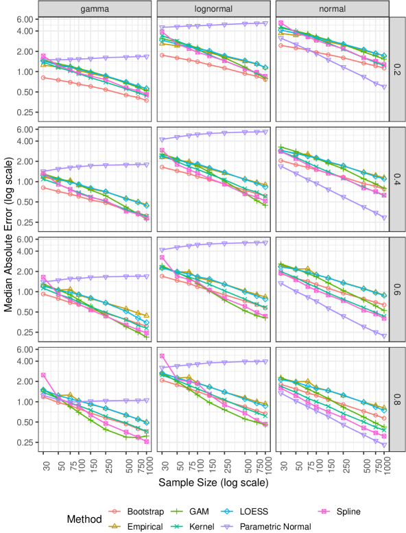
Figure 1: Comparative performance of cutpoint estimation methods on normal and lognormal data.

4 Performance of different cutpoint estimation methods

In order to compare the performance of the different estimation methods, we performed a simulation study similar to the one by Fluss et al. (Fluss et al., 2005). In the present study we used the aforementioned seven different methods (excluding the mean, median and manual methods) to determine the optimal cutpoint for the Youden index. Specifically, we drew samples from three types of distributions (normal, log-normal, and gamma) and at four different levels of separation (Youden index values of 0.2, 0.4, 0.6 and 0.8). In the case of normally distributed data the target separation was achieved by keeping the mean of the control group constant at 100 and manipulating the mean of the experimental group (105.05, 110.49, 116.83 and 125.63). The standard deviation for both groups was constant at 10. In the case of log-normally distributed data the target separation was achieved by keeping the mean of the control group constant at 2.5 and manipulating the mean of the experimental group (2.76, 3.02, 3.34 and 3.78). The standard deviation for both groups was constant at 2.5. In the case of gamma distributed data the target separation was achieved by keeping the rate parameter of the control group constant at 0.5 and manipulating the rate parameter of the experimental group (0.344, 0.233, 0.143, 0.072). The shape parameter for both groups was constant at 2. In all scenarios the prevalence was held constant at 50 percent without loss of generalizability (Leeflang et al., 2008). The overall sample sizes were 30, 50, 75, 100, 150, 250, 500, 750 and 1.000, resulting in 108 different scenarios. For each scenario 10.000 samples were generated. In each sample we compared the optimal cutpoint identified by the different methods to the true optimal cutpoint according to the scenario parameters. To describe the performance, we calculated the median absolute error within the scenarios. Figure 1 shows the performance of the different methods.

Mirroring earlier results (Fluss et al., 2005; Leeflang et al., 2008), the most efficient method to estimate optimal cutpoints depends on the underlying distribution, sample size and level of separation. When the underlying distributions are normal, the Normal method and for small samples bootstrapping yield the best results. However, the Normal method gives erroneous optimal cutpoints with lognormal and gamma distributions. The empirical and LOESS methods show the highest levels of error when the data is normally distributed. In that scenario, the level of error of the empirical method with 1.000 observations is about as high as the error of the Normal method with 30 observations. In scenarios with non-normal distributions either bootstrapping or GAM give the best results. Bootstrapping is better for small levels of separation and small sample sizes while GAM outperforms all other methods for larger levels of separation combined with larger sample sizes. While more work is needed to tease apart the different conditions under which the individual methods are optimal, it seems that more advanced methods are preferable to the empirical method (Fluss et al., 2005; Leeflang et al., 2008; Hirschfeld and do Brasil, 2014).

5 Software

5.1 Overview of functions, classes and data

The package consists of several main functions. Some of these functions may serve as inputs to other functions or may also be used individually, for example the cutpoint estimation methods and roc.

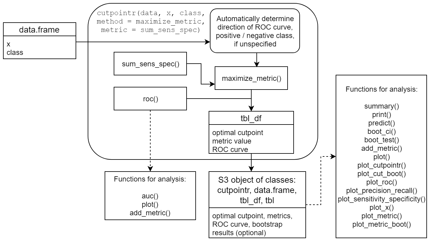
Figure 2: Interplay of functions and classes in cutpointr.

5.1.1 Main functions

The main function of the package is cutpointr. There are two ways to invoke cutpointr. First, the data can be supplied as a data frame in the data argument and the predictor, outcome, and grouping variables then must be given in x, class, and subgroup. This interface uses nonstandard evaluation via the rlang package. For programming purposes, supplied variables can be unquoted using !!. Second, the data argument can be left as NULL and the predictor, outcome, and grouping variables then have to be supplied as raw vectors of any suitable type. Further arguments control the choice of estimation method, which metric shall be optimized, if bootstrapping should be run and more. Arguments to these downstream functions are passed to ... directly in cutpointr. Some methods are prefixed with oc_ to make them distinguishable from metrics, the maximization and minimization methods are not. The functions for calculating metrics and for finding cutpoints can easily be user-defined. For example, the function that is supplied as the metric argument should return a numeric vector, a matrix, or a data frame with one column. If the column is named, the name will be included in the output and plots. The inputs are vectors of $TP$, $FP$, $TN$ and $FN$. See vignette("cutpointr") for more details on how to write functions that are suitable inputs for method or metric. For a complete overview of metrics included in cutpointr see table 2.

The multi_cutpointr function is a wrapper that by default runs cutpointr using all numeric columns in data as predictors, except for the class column, or using the columns in the x argument. All other arguments are simply passed to cutpointr. The rows of the resulting data frame represent the output of cutpointr per predictor variable. There is a summary method for objects of class multi_cutpointr, however the plotting functions do not support multi_cutpointr objects.

Both cutpointr and multi_cutpointr return ROC curves. If bootstrapping was run, also ROC curves based on the in- and out-of-bag observations are returned within the boot column. Internally, the roc function is used which is also exported so that it can be used on its own if only a ROC curve is desired. It returns the ROC curve as a data.frame with all unique cutpoints and the associated numbers of correct and false classifications, the associated rates and the obtained metric value in the column m as calculated using the function in the metric argument. The results can be inspected for example with summary, plot or plot_cutpointr. The latter function allows for flexibly plotting metrics per cutpoint or against each other, including confidence intervals if bootstrapping was run.

5.1.2 Classes

The object returned by cutpointr is an object of the classes cutpointr, tbl_df, tbl, and data.frame. It is returned and printed unaltered as a tbl_df to make sure that the output is comprehensible at a glance, clearly arranged, and also easy to pass to subsequent functions. In addition to the model parameters and some metrics, the object also includes data frames in list columns that contain the original data and the ROC curve. If a subgroup was defined, the aforementioned data are split per subgroup and returned in the respective rows. The ROC curve is returned as a nested data frame in the roc_curve column with the metric at each cutpoint x.sorted in the m column. If bootstrapping was run, the boot column contains a data frame with the bootstrap results. Each row represents one bootstrap repetition. For each repetition, the AUC, the metric in metric, several other metrics, the numbers of true or false classifications and the in- and out-of-bag ROC curves, again in nested data frames, are returned. For all of these metrics cutpointr returns the in- and out-of-bag value, as indicated by the suffix _b or _oob. The output of the summary method for cutpointr objects is an object of the classes summary_cutpointr, tbl_df, tbl and data.frame.

The object returned by multi_cutpointr is an object of the classes multi_cutpointr, tbl_df, tbl, and data.frame that has a corresponding summary method, but no plotting methods. The roc function also returns a tbl_df that carries an additional roc_cutpointr class.

5.1.3 Data

The data set suicide which is suitable for running binary classification tasks is included in cutpointr. Various personality and clinical psychological characteristics of 532 participants were assessed as part of an online-study determining optimal cutpoints (Glischinski et al., 2016). To identify persons at risk for attempting suicide, various demographic and clinical characteristics were assessed. Depressive Symptom Inventory - Suicidality Subscale (DSI-SS) sum scores and whether the subject had previously attempted suicide were recorded. Two additional demographic variables (age and gender) are also included to test estimation of different cutpoints per subgroup.

6 Example: Suicide dataset

To showcase the functionality, we’ll use the included suicide data set and calculate possible cutpoints for the DSI-SS. To estimate a cutpoint maximizing $Se+Sp$, various in-sample metrics, and the ROC-curve cutpointr can be run with minimal inputs.

R> library("cutpointr") R> opt_cut <- cutpointr(suicide, dsi, suicide, silent = TRUE) R> opt_cut

# A tibble: 1 x 16 direction optimal_cutpoint method sum_sens_spec acc sensitivity <chr> <dbl> <chr> <dbl> <dbl> <dbl> 1 >= 2 maximize_metric 1.75179 0.864662 0.888889 specificity AUC pos_class neg_class prevalence outcome predictor <dbl> <dbl> <fct> <fct> <dbl> <chr> <chr> 1 0.862903 0.923779 yes no 0.0676692 suicide dsi data roc_curve boot <list<df[,2]>> <list> <lgl> 1 [532 x 2] <tibble [13 x 10]> NA

The determined “optimal” cutpoint in this case is 2, thus all subjects with a score of at least 2 would be classified as positives, indicating a history of at least one suicide attempt. Based on this sample, this leads to a sum of $Se$ and $Sp$ of 1.75. Furthermore, we receive outputs that are independent of the determined cutpoint such as the AUC, the prevalence, or the ROC curve.

cutpointr makes assumptions about the direction of the dependency between class and x based on the median, if direction and / or pos_class and neg_class are not specified. Thus, the same result can be achieved by manually defining direction and the positive / negative classes which is slightly faster:

R> cutpointr(suicide, dsi, suicide, direction = ">=", pos_class = "yes",
+    neg_class = "no", method = maximize_metric, metric = sum_sens_spec)

To receive additional descriptive statistics, summary can be run on the cutpointr object (output omitted).

6.0.1 Reproducible Bootstrapping and parallelization

If boot_runs is larger than zero, cutpointr will carry out the usual cutpoint calculation on the full sample, just as before, and additionally on boot_runs bootstrap samples. The bootstrapping can be parallelized by setting allowParallel = TRUE and starting a parallel backend. Internally, the parallelization is carried out using foreach (Microsoft and Weston, 2017) and doRNG (Gaujoux, 2017) for reproducible parallel loops. An example of a suitable parallel backend is a SOCK cluster that can be started using the snow package (Tierney et al., 2009). Reproducibility can be achieved by setting a seed using set.seed, both in the case of sequential or parallel execution.

R> library("doSNOW")
R> library("tidyverse")
R> cl <- makeCluster(2) # 2 cores
R> registerDoSNOW(cl)
R> set.seed(100)
R> opt_cut_b <- cutpointr(suicide, dsi, suicide, boot_runs = 1000,
+    silent = TRUE, allowParallel = TRUE)
R> stopCluster(cl)
R> opt_cut_b %>% select(optimal_cutpoint, data, boot)

# A tibble: 1 x 3 optimal_cutpoint data boot <dbl> <list<df[,2]>> <list> 1 2 [532 x 2] <tibble [1,000 x 23]>

The returned object includes a nested data frame in the column boot that contains the optimal cutpoint per bootstrap sample along with the metric calculated using the function in metric and various additional metrics. The metrics are suffixed by _b to indicate in-bag results or _oob to indicate out-of-bag results. Now we receive a larger summary and additional plots upon applying summary and plot (see figure 3).

R> summary(opt_cut_b)

Method: maximize_metric
Predictor: dsi
Outcome: suicide
Direction: >=
Nr. of bootstraps: 1000

    AUC   n n_pos n_neg
 0.9238 532    36   496

 optimal_cutpoint sum_sens_spec    acc sensitivity specificity tp fn fp  tn
                2        1.7518 0.8647      0.8889      0.8629 32  4 68 428

Predictor summary:
        Min.   5% 1st Qu. Median  Mean 3rd Qu.  95% Max.    SD NAs
overall    0 0.00       0      0 0.921       1 5.00   11 1.853   0
no         0 0.00       0      0 0.633       0 4.00   10 1.412   0
yes        0 0.75       4      5 4.889       6 9.25   11 2.550   0

Bootstrap summary:
          Variable  Min.    5% 1st Qu. Median  Mean 3rd Qu.   95%  Max.    SD
  optimal_cutpoint 1.000 1.000   2.000  2.000 2.078   2.000 4.000 4.000 0.668
             AUC_b 0.832 0.878   0.907  0.926 0.923   0.941 0.960 0.981 0.025
           AUC_oob 0.796 0.867   0.901  0.923 0.924   0.955 0.974 0.990 0.034
   sum_sens_spec_b 1.552 1.661   1.722  1.760 1.757   1.794 1.837 1.925 0.054
 sum_sens_spec_oob 1.393 1.569   1.667  1.724 1.722   1.782 1.867 1.905 0.089
             acc_b 0.724 0.776   0.852  0.867 0.860   0.880 0.904 0.942 0.035
           acc_oob 0.704 0.763   0.845  0.862 0.855   0.879 0.900 0.928 0.038
     sensitivity_b 0.657 0.808   0.865  0.903 0.900   0.938 0.974 1.000 0.052
   sensitivity_oob 0.500 0.688   0.818  0.875 0.868   0.929 1.000 1.000 0.097
     specificity_b 0.709 0.762   0.849  0.864 0.857   0.878 0.908 0.951 0.039
   specificity_oob 0.691 0.751   0.845  0.861 0.854   0.879 0.911 0.948 0.044
    cohens_kappa_b 0.174 0.280   0.367  0.414 0.410   0.456 0.525 0.643 0.072
  cohens_kappa_oob 0.125 0.247   0.336  0.390 0.388   0.443 0.520 0.641 0.082

R> plot(opt_cut_b)

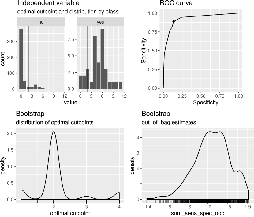
Figure 3: Main plotting function of cutpointr, the top left showing the distribution of the predictor values per class, the top right showing the ROC-curve, the bottom left showing the bootstrapped cutpoint variability, and the bottom right showing the distribution of the out-of-bag metric values.

This allows us to form expectations about the performance on unseen data and to compare these expectations to the in-sample performance. First, the cutpoints that are obtained via the chosen method - maximizing the sum of sensitivity and specificity - are quite stable here. In the majority of bootstrap samples (777 out of 1000 times) the chosen cutpoint is 2 as can be estimated from the plot or simply by inspecting the results, for example using opt_cut_b %>% select(boot) %>% unnest(boot) %>% count(optimal_cutpoint). 2 is also the cutpoint that was determined on the full sample. Second, the distribution of the out-of-bag performance, namely $Se+Sp$, can be assessed from the plot. Summary statistics for the in- and out-of-bag metrics are returned by the summary function, for example the first and third quartiles of the out-of-bag values of $Se+Sp$ are 1.67 and 1.78, respectively, which could also be calculated with boot_ci(opt_cut_b, sum_sens_spec, in_bag = FALSE, alpha = 0.5). Furthermore, since both in- and out-of-bag results are returned, we can confirm the optimism of the in-sample performance estimation. The median of the in-bag metric is 1.76 while the median of the out-of-bag metric is 1.72. The optimal cutpoint of 2 yields $Se+Sp=1.75$ on the full sample. The other metrics can be compared in a similar fashion. Third, to inspect the in-sample fit, the chosen cutpoint is displayed on a histogram of the predictor per class and on the ROC-curve.

The individual plots can be reproduced using plot_x, plot_roc, plot_cut_boot and plot_metric_boot. Another way of inspecting the selection of the optimal cutpoint is to plot all possible cutpoints along with the corresponding metric values. This can be achieved using the plot_metric function which also plots bootstrapped confidence intervals of the in-sample metric at each cutpoint, if bootstrapping was run (see figure 4).

R> plot_metric(opt_cut_b, conf_lvl = 0.95) +
+    ylab("Sensitivity + Specificity") +
+    theme_bw()

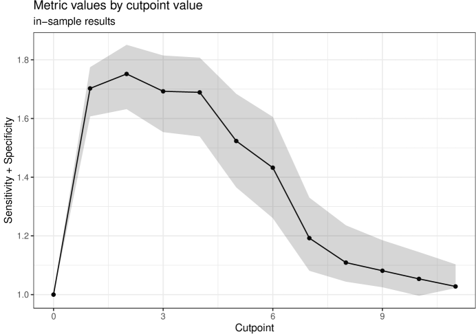
Figure 4: Values of the metric function per cutpoint with 95 percent bootstrap confidence interval.

6.0.2 Subgroups

If the data contains a grouping variable that is assumed to play a role in determining the cutpoint, the complete selection and validation procedure can be conveniently run on separate subgroups by specifying the subgroup argument.

R> set.seed(100)
R> opt_cut_b_g <- cutpointr(suicide, dsi, suicide, gender, boot_runs = 1000,
+    boot_stratify = TRUE, pos_class = "yes", direction = ">=")
R> opt_cut_b_g %>% select(subgroup, optimal_cutpoint, sum_sens_spec, data)

# A tibble: 2 x 4 subgroup optimal_cutpoint sum_sens_spec data <chr> <dbl> <dbl> <list<df[,2]>> 1 female 2 1.80812 [392 x 2] 2 male 3 1.62511 [140 x 2]

This time the output contains one row per subgroup. In this case, we receive different optimal cutpoints for the female and male group. As we can also see from the in-sample results, the performance seems to be superior in the female group. To confirm this, we can again inspect the summary, particularly the bootstrap results.

R> summary(opt_cut_b_g)

Method: maximize_metric
Predictor: dsi
Outcome: suicide
Direction: >=
Subgroups: female, male
Nr. of bootstraps: 1000

Subgroup: female
--------------------------------------
[...]
Bootstrap summary:
          Variable  Min.    5% 1st Qu. Median  Mean 3rd Qu.   95%  Max.    SD
[...]
 sum_sens_spec_oob 1.338 1.609   1.729  1.783 1.779   1.864 1.903 1.945 0.095
[...]

Subgroup: male
-------------------------------------
[...]
Bootstrap summary:
          Variable  Min.    5% 1st Qu. Median  Mean 3rd Qu.   95%  Max.    SD
[...]
 sum_sens_spec_oob 0.786 0.981   1.332  1.504 1.479   1.659 1.860 2.000 0.248
[...]

The out-of-bag value of the mean of the sum of sensitivity and specificity in the female group is about 0.29 larger than in the male group. Additionally, the selected cutpoints by simple maximization are less variable in the female group (see also figure 5).

R> plot(opt_cut_b_g)

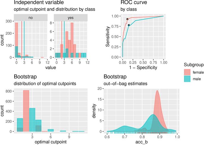
Figure 5: Main plotting function of cutpointr with subgroups showing the distribution of the predictor values per class, the ROC-curve, the bootstrapped cutpoint variability, and the distribution of the out-of-bag metric values.

The higher predictive performance of the predictor variable in the female group is furthermore emphasized by the larger AUC. The summary of AUC_b summarizes the AUC in all bootstrap samples which can be informative for comparing the general predictive ability of the predictor variable in all subgroups.

The observed variability of the selected cutpoints showcases the need for methods that estimate optimal cutpoints with less variability. cutpointr offers maximize_boot_metric, minimize_boot_metric, maximize_gam_metric, minimize_gam_metric, maximize_spline_metric, minimize_spline_metric, maximize_loess_metric, minimize_loess_metric, oc_youden_normal and oc_youden_kernel for that purpose. Since we can not assume the predictor in the positive and negative class to be normally distributed, we will use the Kernel method for determining optimal cutpoints to maximize the Youden index. In our experience, the Kernel method is more suitable for data with a small number of unique predictor values than the smoothing methods. The function oc_youden_kernel does not return a metric value at the estimated cutpoint on its own, but instead the estimated cutpoint is applied to the ROC curve, see chapter 2.2. The function in metric is only used for validation purposes so that we can compare these results to the previous ones.

R> set.seed(100)
R> opt_cut_k_b_g <- cutpointr(suicide, dsi, suicide, gender,
+    method = oc_youden_kernel, metric = sum_sens_spec, boot_runs = 1000)
R> summary(opt_cut_k_b_g)

Method: oc_youden_kernel
Predictor: dsi
Outcome: suicide
Direction: >=
Subgroups: female, male
Nr. of bootstraps: 1000

Subgroup: female
--------------------------------------
[...]
Bootstrap summary:
          Variable  Min.    5% 1st Qu. Median  Mean 3rd Qu.   95%  Max.    SD
[...]
 sum_sens_spec_oob 1.338 1.590   1.741  1.792 1.785   1.873 1.906 1.945 0.102
[...]

Subgroup: male
-------------------------------------
[...]
Bootstrap summary:

          Variable  Min.    5% 1st Qu. Median  Mean 3rd Qu.   95%  Max.    SD
[...]
 sum_sens_spec_oob 0.732 0.975   1.378  1.542 1.537   1.787 1.857 2.000 0.263
[...]

The plot of opt_cut_k_b_g (not shown) reveals that the determined cutpoints are again much less variable in the female than in the male group. Since the Kernel method should exhibit a lower variability than the previously used maximization method, we expect better validation results in the bootstrapping. Indeed, in both subgroups $Se+Sp$ in the out-of-bag observations is slightly larger than before with the nonparametric empirical method (for example, the mean of $Se+Sp$ in the male group is 1.54 here instead of 1.48).

6.0.3 Alternative metric function

Various alternative metric functions are available and in the example dataset it is reasonable to assign different costs to false positives and false negatives. A false positive may lead to someone being treated without an urgent need to do so, while a false negative may lead to someone not being treated who may attempt suicide or suffer from a considerably lower quality of life. cutpointr offers the possibility to define these separate costs using the misclassification_cost metric. Since we want to minimize the costs we use the minimize_metric function as method. If also separate utilities for true positives and true negatives should be defined, we could use the total_utility function. In practice, the ratio of the costs or the actual costs may be known exactly but for the purpose of this example we assume that a false negative is ten times more costly than a false positive. Incidentally, this leads to cutpoints that are comparable to the previously obtained ones.

R> set.seed(100)
R> opt_cut_c_g_b <- cutpointr(suicide, dsi, suicide, gender,
+    method = minimize_metric, metric = misclassification_cost, cost_fp = 1,
+    cost_fn = 10, pos_class = "yes", direction = ">=", boot_runs = 1000)
R> opt_cut_c_g_b %>%
+    select(subgroup, optimal_cutpoint, misclassification_cost)

# A tibble: 2 x 3 subgroup optimal_cutpoint misclassification_cost <chr> <dbl> <dbl> 1 female 2 63 2 male 3 40

6.1 Midpoints as optimal cutpoints

So far - which is the default in cutpointr - we have considered all unique values of the predictor as possible cutpoints. An alternative could be to use a sequence of equidistant values instead, for example in the preceding application all integers in $[0,12]$ and the additional cutpoint $Inf$ to allow for classifying all observations as negative. However, in the case of very sparse data and small intervals between the defined candidate cutpoints (i.e., a “dense” sequence like seq(0, 12, by = 0.01)) this leads to the uninformative evaluation of large ranges of cutpoints that all result in the same metric value. A more elegant alternative, not only for the case of sparse data, that is supported by cutpointr is the use of a mean value of the optimal cutpoint and the next highest (if direction = ">=") or the next lowest (if direction = "<=") predictor value in the data. The result is an optimal cutpoint that is equal to the cutpoint that would be obtained using an infinitely dense sequence of candidate cutpoints and is thus more computationally efficient. This behavior can be activated by setting use_midpoints = TRUE. If we use this setting, we obtain an optimal cutpoint of 1.5 for the complete sample on the suicide data instead of 2 when maximizing $Se+Sp$. In practice, this would not make a difference here as the DSI-SS takes on only integer values.

Furthermore, not using midpoints but the values found in the data may lead to a positive or negative bias of the estimation procedure, depending on direction. For example, if direction = ">=" and use_midpoints = FALSE, the returned optimal cutpoint represents the highest possible cutpoint that leads to the optimal metric, because all values that are below the optimal cutpoint and are larger than the next lowest value in the data result in the same metric value. This bias only applies to estimation methods that use the ROC curve for selecting a cutpoint and are mainly relevant with small and sparse data. See vignette("cutpointr") for more details and some simulation results regarding the bias and its reduction using midpoints.

6.2 Benchmarks

To offer a comparison to established solutions, cutpointr 1.0.0 was benchmarked against optimal.cutpoints from OptimalCutpoints 1.1-4 (López-Ratón et al., 2014), thres2 from ThresholdROC 2.7 (Perez-Jaume et al., 2017), a custom function using the functions prediction and performance from ROCR 1.0-7 (Sing et al., 2005) and a custom function using roc from pROC v1.15.0 (Robin et al., 2011) with the setting algo = 2 which is the fastest one in this application. As the results will be identical for empirical maximization and more advanced methods are not included in most other packages, the benchmark focuses on a timing comparison. By generating data sets of different sizes, the benchmarks offer a comparison of the scalability of the different solutions and their performance on small and larger data.

The benchmarking was carried out unparallelised on Windows 10 v10.0.17763 Build 17763 with a 6-Core AMD CPU at 4GHz and 32GB of memory running R 3.6.0. The runtime of the functions was assessed using microbenchmark (Mersmann, 2018). The values of the predictor variable were drawn from a normal distribution, leading to a number of possible cutpoints that is close or equal to the sample size. Accordingly, the search for an optimal cutpoint is relatively demanding.

Benchmarks are run for sample sizes of 100, 1000, 10000, $1e5$, $1e6$, and $1e7$. In small samples cutpointr is slower than the other packages. This disadvantage seems to be caused mainly by certain functions from tidyr that are used to nest the input data and produce the compact output. The C++ functions in cutpointr lead to a sizeable speedup with larger data, but some are slightly slower with small data. While the speed disadvantage with small data should be of low practical importance, since it usually amounts to only minimal delays, cutpointr scales more favorably than the other solutions and is the fastest solution for sample sizes $\geq 1e6$. For data as large as $1e7$ observations cutpointr takes about 70% of the runtime of ROCR and pROC. This phenomenon is illustrated also by the performance in the task of ROC curve calculation, in which roc from cutpointr is fast also in small samples but has an advantage over ROCR and pROC again only in larger samples (see figure 6).

All of cutpointr, pROC and ROCR are generally faster than OptimalCutpoints and ThresholdROC with the exception of small samples. OptimalCutpoints and ThresholdROC had to be excluded from benchmarks with more than 10000 observations due to high memory requirements. Upon inspection of the source code of the different packages, it seems that the differences in speed and memory consumption are mainly due to the way the ROC curve is built or whether a ROC curve is built at all. A search over the complete vector of predictor values is obviously inefficient, so a search over the points on the ROC curve (which represent combinations of $Se$ and $Sp$ for all unique predictor values) will offer a faster solution. For building the ROC curve, a binary vector representing whether an observation is a $TP$ can be sorted according to the order of the predictor variable and cumulatively summed up. The solutions by cutpointr and ROCR rely on this algorithm.

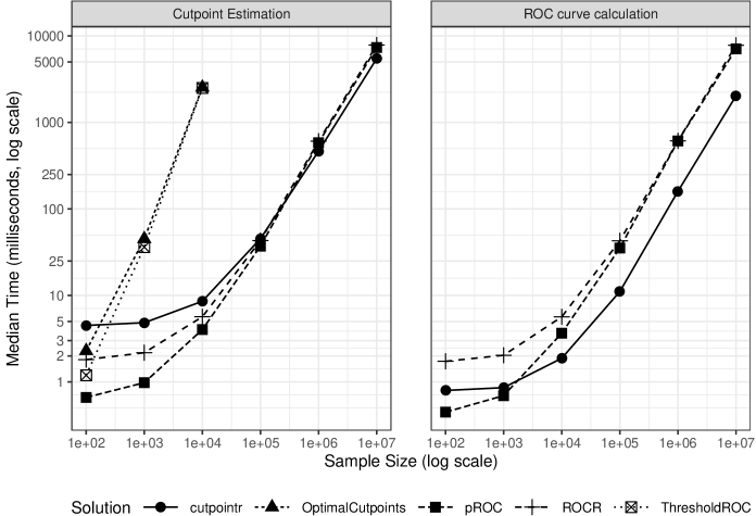
Figure 6: Benchmark results.

7 Conclusion

The aim in developing cutpointr was to make improved methods to estimate and validate optimal cutpoints available. While there are already several packages that aid the calculation of a wide range of metrics (López-Ratón et al., 2014, 2017; Perez-Jaume et al., 2017), some of these rely on suboptimal procedures to estimate a cutpoint. Most use the empirical method, which is prone to high variability an to overestimating the diagnostic utility of optimal cutpoints. cutpointr incorporates several methods to choose cutpoints that are not necessarily optimal in the specific sample but perform relatively well in the population from which the sample was drawn and are more stable.

It is beyond the scope of the present manuscript to determine the best estimation method, since this will likely depend on characteristics of the study as well as the chosen metric. However, we believe that cutpointr may prove useful for simulation studies because of its scalability as well as applied research because of its ability to estimate the cutpoint variability and out-of-sample performance.

8 Acknowledgements

The study was supported by the German Federal Ministry for Education and Research to GH (BMBF #01EK1501).

References

- Altman et al. (1994) Altman DG, Lausen B, Sauerbrei W, Schumacher M (1994). “Dangers of Using “Optimal” Cutpoints in the Evaluation of Prognostic Factors.” JNCI: Journal of the National Cancer Institute, 86(11), 829–835. ISSN 0027-8874. 10.1093/jnci/86.11.829. URL https://academic.oup.com/jnci/article/86/11/829/955201/Dangers-of-Using-Optimal-Cutpoints-in-the.
- Altman and Royston (2000) Altman DG, Royston P (2000). “What Do We Mean by Validating a Prognostic Model?” Statistics in Medicine, 19(4), 453–473.
- Arlot and Celisse (2010) Arlot S, Celisse A (2010). “A Survey of Cross-Validation Procedures for Model Selection.” Statistics Surveys, 4, 40–79. URL https://hal-ens.archives-ouvertes.fr/docs/00/40/79/06/PDF/preprintLilleArlotCelisse.pdf.
- Breiman (1996) Breiman L (1996). “Bagging Predictors.” Machine Learning, 24(2), 123–140. URL http://www.springerlink.com/index/L4780124W2874025.pdf.
- Breiman (2001) Breiman L (2001). “Random Forests.” Machine Learning, 45(1), 5–32. URL http://www.springerlink.com/index/U0P06167N6173512.pdf.
- Buja et al. (1989) Buja A, Hastie T, Tibshirani R (1989). “Linear Smoothers and Additive Models.” The Annals of Statistics, pp. 453–510.
- Carpenter and Bithell (2000) Carpenter J, Bithell J (2000). “Bootstrap Confidence Intervals: When, Which, What? A Practical Guide for Medical Statisticians.” Statistics in Medicine, 19(9), 1141–1164. ISSN 1097-0258. 10.1002/(SICI)1097-0258(20000515)19:9<1141::AID-SIM479>3.0.CO;2-F. URL https://onlinelibrary.wiley.com/doi/abs/10.1002/%28SICI%291097-0258%2820000515%2919%3A9%3C1141%3A%3AAID-SIM479%3E3.0.CO%3B2-F.
- Dougherty et al. (2010) Dougherty ER, Sima C, Hanczar B, Braga-Neto UM, others (2010). “Performance of Error Estimators for Classification.” Current Bioinformatics, 5(1), 53–67. URL http://www.ingentaconnect.com/content/ben/cbio/2010/00000005/00000001/art00005.
- Efron and Tibshirani (1997) Efron B, Tibshirani R (1997). “Improvements on Cross-Validation: The. 632+ Bootstrap Method.” Journal of the American Statistical Association, 92(438), 548.
- Ewald (2006) Ewald B (2006). “Post Hoc Choice of Cut Points Introduced Bias to Diagnostic Research.” Journal of Clinical Epidemiology, 59(8), 798–801. ISSN 0895-4356, 1878-5921. 10.1016/j.jclinepi.2005.11.025. URL http://www.jclinepi.com/article/S0895435606000308/abstract.
- Faraggi and Reiser (2002) Faraggi D, Reiser B (2002). “Estimation of the Area Under the ROC Curve.” Statistics in Medicine, 21(20), 3093–3106. URL http://onlinelibrary.wiley.com/doi/10.1002/sim.1228/full.
- Fluss et al. (2005) Fluss R, Faraggi D, Reiser B (2005). “Estimation of the Youden Index and its Associated Cutoff Point.” Biometrical Journal, 47(4), 458–472. URL http://onlinelibrary.wiley.com/doi/10.1002/bimj.200410135/full.
- Gaujoux (2017) Gaujoux R (2017). “\pkgdoRNG: Generic Reproducible Parallel Backend for \codeforeach Loops.” \proglangR package version 1.7.1. URL https://CRAN.R-project.org/package=doRNG.
- Glischinski et al. (2016) Glischinski M, Teismann T, Prinz S, Gebauer JE, Hirschfeld G (2016). “Depressive Symptom Inventory Suicidality Subscale: Optimal Cut Points for Clinical and Non-Clinical Samples.” Clinical psychology & psychotherapy, 23(6), 543–549.
- Hirschfeld and do Brasil (2014) Hirschfeld G, do Brasil PEAA (2014). “A Simulation Study into the Performance of “Optimal” Diagnostic Thresholds in the Population:“Large” Effect Sizes are not Enough.” Journal of Clinical Epidemiology, 67(4), 449–453. URL http://www.sciencedirect.com/science/article/pii/S089543561300348X.
- Hirschfeld and Thielsch (2015) Hirschfeld G, Thielsch MT (2015). “Establishing Meaningful Cut Points for Online User Ratings.” Ergonomics, 58(2), 310–320. ISSN 0014-0139. 10.1080/00140139.2014.965228. URL http://dx.doi.org/10.1080/00140139.2014.965228.
- Hurvich et al. (1998) Hurvich CM, Simonoff JS, Tsai CL (1998). “Smoothing Parameter Selection in Nonparametric Regression Using an Improved Akaike Information Criterion.” Journal of the Royal Statistical Society: Series B (Statistical Methodology), 60(2), 271–293. URL http://onlinelibrary.wiley.com/doi/10.1111/1467-9868.00125/full.
- Leeflang et al. (2008) Leeflang MM, Moons KG, Reitsma JB, Zwinderman AH (2008). “Bias in Sensitivity and Specificity Caused by Data-Driven Selection of Optimal Cutoff Values: Mechanisms, Magnitude, and Solutions.” Clinical Chemistry, (4), 729–738.
- López-Ratón et al. (2017) López-Ratón M, Molanes-López EM, Letón E, Cadarso-Suárez C (2017). “\pkgGsymPoint: An \proglangR Package to Estimate the Generalized Symmetry Point, an Optimal Cut-off Point for Binary Classification in Continuous Diagnostic Tests.” R Journal, 9(1), 262–283.
- López-Ratón et al. (2014) López-Ratón M, Rodríguez-Álvarez MX, Cadarso-Suárez C, Gude-Sampedro F (2014). “\pkgOptimalCutpoints: An \proglangR Package for Selecting Optimal Cutpoints in Diagnostic Tests.” Journal of Statistical Software, 061(i08). URL http://econpapers.repec.org/article/jssjstsof/v_3a061_3ai08.htm.
- Mersmann (2018) Mersmann O (2018). \pkgmicrobenchmark: Accurate Timing Functions. \proglangR package version 1.4-4, URL https://CRAN.R-project.org/package=microbenchmark.
- Microsoft and Weston (2017) Microsoft, Weston S (2017). \pkgforeach: Provides Foreach Looping Construct for \proglangR. \proglangR package version 1.4.4, URL https://CRAN.R-project.org/package=foreach.
- Molinaro et al. (2005) Molinaro AM, Simon R, Pfeiffer RM (2005). “Prediction Error Estimation: A Comparison of Resampling Methods.” Bioinformatics, 21(15), 3301–3307.
- Perez-Jaume et al. (2017) Perez-Jaume S, Skaltsa K, Pallarès N, Carrasco JL (2017). “\pkgThresholdROC: Optimum Threshold Estimation Tools for Continuous Diagnostic Tests in \proglangR.” Journal of Statistical Software, 82(1), 1–21.
- R Core Team (2018) R Core Team (2018). \proglangR: A Language and Environment for Statistical Computing. \proglangR Foundation for Statistical Computing, Vienna, Austria. URL https://www.R-project.org/.
- Robin et al. (2011) Robin X, Turck N, Hainard A, Tiberti N, Lisacek F, Sanchez JC, Müller M (2011). “\pkgpROC: An Open-Source Package for \proglangR and \proglangS+ to Analyze and Compare ROC Curves.” BMC bioinformatics, 12(1), 77. URL https://bmcbioinformatics.biomedcentral.com/articles/10.1186/1471-2105-12-77.
- Sing et al. (2005) Sing T, Sander O, Beerenwinkel N, Lengauer T (2005). “\pkgROCR: Visualizing Classifier Performance in \proglangR.” Bioinformatics, 21(20), 3940–3941. URL https://academic.oup.com/bioinformatics/article-abstract/21/20/3940/202693.
- Steyerberg et al. (2001) Steyerberg EW, Borsbooma GJ, Eijkemansa MR, Vergouwea Y, Habbemaa JDF (2001). “Internal Validation of Predictive Models: Efficiency of Some Procedures for Logistic Regression Analysis.” Journal of Clinical Epidemiology, 54, 774–781.
- Tierney et al. (2009) Tierney L, Rossini AJ, Li N (2009). “\pkgSnow: A Parallel Computing Framework for the \proglangR System.” International Journal of Parallel Programming, 37(1), 78–90. URL http://www.springerlink.com/index/3v37mg0k63053567.pdf.
- Wand and Ripley (2015) Wand MP, Ripley BD (2015). \pkgKernSmooth: Functions for Kernel Smoothing for Wand and Jones. \proglangR package version 2.23-15. URL https://CRAN.R-project.org/package=KernSmooth.
- Wang (2010) Wang XF (2010). “\pkgfANCOVA: Nonparametric Analysis of Covariance.” \proglangR package version 0.5-1. URL https://CRAN.R-project.org/package=fANCOVA.
- Wickham et al. (2014) Wickham H, et al. (2014). “Tidy Data.” Journal of Statistical Software, 59(10), 1–23.
- Wood (2001) Wood SN (2001). “\pkgmgcv: GAMs and Generalized Ridge Regression for \proglangR.” \proglangR news, 1(2), 20–25.