An Evolutionary Deep Learning Method for Short-term Wind Speed Prediction: A Case Study of the Lillgrund Offshore Wind Farm

Abstract

Accurate short-term wind speed forecasting is essential for large-scale integration of wind power generation. However, the seasonal and stochastic characteristics of wind speed make forecasting a challenging task. This study uses a new hybrid evolutionary approach that uses a popular evolutionary search algorithm, CMA-ES, to tune the hyper-parameters of two long-term-short-term (LSTM) ANN models for wind prediction.

The proposed hybrid approach is trained on data gathered from an offshore wind turbine installed in a Swedish wind farm located in the Baltic Sea. Two forecasting horizons including ten-minutes ahead (absolute short term) and one-hour ahead (short term) are considered in our experiments. Our experimental results indicate that the new approach is superior to five other applied machine learning models, i.e., polynomial neural network (PNN), feed-forward neural network (FNN), nonlinear autoregressive neural network (NAR) and adaptive neuro-fuzzy inference system (ANFIS), as measured by five performance criteria.

Keywords Wind speed prediction model $\cdot$ short-term forecasting $\cdot$ evolutionary algorithms $\cdot$ deep learning  $\cdot$ sequential deep learning  $\cdot$ long short term memory neural network $\cdot$ hybrid evolutionary deep learning method  $\cdot$ covariance matrix adaptation evolution strategy.

1 Introduction

Concerning trajectories for global warming and environmental pollution have motivated intensive efforts to replace fossil fuels[1]. One of the most important clean energy sources is wind. Wind energy has key advantages in terms of technological maturity, cost, and life-cycle greenhouse gas emissions[2]. However, wind is a variable resource, so accurate wind power forecasts are crucial in reducing the incidence of costly curtailments, and in protecting system integrity and worker-safety[3]. However, obtaining an accurate local wind speed prediction can be difficult. This is because the wind speed characteristics are stochastic, intermittent and non-stationary which can defeat simple models[4].

In this paper, we propose a hybrid evolutionary deep forecasting model combining a recurrent deep learning model (LSTM network)[5], coupled with the CMA-ES algorithm[6], (called CMAES-LSTM) for predicting the short-term wind speed with high accuracy.

As there is no straightforward theory governing the design of an LSTM network for a given problem[7], we tune model structure and hyper-parameters using a combination of grid search and CMA-ES. We demonstrate the performance of the proposed hybrid (CMAES-LSTM) model using a real case study using data collected from the Lillgrund offshore wind-farm to predict wind speeds ten-minutes ahead and one hour ahead. The proposed method is compared with the FNN model, ANFIS model, PNN model, NAR model and a static LSTM model. Statistical analyses show that the proposed adaptive method exhibits better performance than these current (static) models.

The remainder this article is structured as follows. The next section briefly surveys related work in the field of predictive wind models. Section 3 presents current methodologies, theories and our proposed hybrid evolutionary deep learning (CMAES-LSTM) model. Section 4 exhibits the performance indices applied for evaluating the introduced models. After this, Section 5 gives a brief description of the offshore wind farm applied in this paper. Section 6 describes and analyses our experimental results. Lastly, we provide a summary and outline future work in Section 7.

2 Related Work

Today, wind turbine generators (WTGs) are installed in onshore, nearshore and offshore areas worldwide[8, 9, 10, 11]. Sweden is one of the leading countries harnessing offshore wind power due to its geographical location, access to shallow seas and strong North winds on the Baltic Sea. Wind energy is variable wind resources that are influenced by several factors including: the location of the turbines (on-, near-, offshore); turbine height; seasons, meso-scale and diurnal variations; and climate change. All of which can affect the stable operation of the power grid [12]. Studies have shown how these factors can impact on the the reliability of wind energy[13].

The short-term predictive models of wind speed based on historical data have been developed using autoregressive moving average models [14], autoregressive integrated moving average models [15]. Related work by Gani et. al.[16] combined non-linear models with support vector machines. Wind forecast methodologies using ANNs include Elman neural networks [17], polynomial neural networks (PNN)[18], feed-forward neural networks (FNN)[19] and long short-term memory Network (LSTM)[7], hybrid artificial neural network[20].

Recently deep-learned ANNs solutions for wind forecasting have proven popular. Hu et al. [21] used transfer learning for short term prediction. Wang et al. [22] introduced a new wind speed forecasting approach using a deep belief network (DBN) based on the deterministic and probabilistic variables. Liu used recurrent deep learning models based on Long Short Term Memory (LSTM) network for forecasting wind speed in different time-scales [23, 24]. Chen et al.  [25] recommended an ensemble of six different LSTM networks configurations for wind speed forecasting with ten-min and one-hour interval. More broadly hybrid nonlinear forecasting models have been explored for the prediction of wind energy generation, solar energy forecasting and energy market forecasting [26, 27, 28, 29, 30, 31].

The work in this paper differs from the previous work in wind-prediction in the use of global heuristic search methods to optimise both network structure and tune hyper-parameters. Our approach customises known methodologies from neuro-evolution[32] to improve the performance of predictive wind models.

3 Methodology

In this section, we introduce the proposed methodologies and related concepts, including LSTM network details, CMA-ES and the combined LSTM network and the CMA-ES algorithm.

3.1 Long short-term memory network (LSTM)

An LSTM is a type of recurrent neural network (RNN) which has the capacity to model time series data with different long-term and short-term dependencies [5]. The core of the LSTM network is the memory cell, which regards the hidden layers place of the of traditional neurons LSTM is equipped with three gates (input, output and forget gates), therefore it is able to add or remove information to the cell state. For calculating the estimated outputs and updating the state of the cell, the following equations can be used:

$$i_{t}=\sigma(W_{ix}x_{t}+W_{im}m_{t-1}+W_{ic}c_{t-1}+b_{i})$$ (1)

$$i_{t}=\sigma(W_{fx}x_{t}+W_{fm}m_{t-1}+W_{fc}c_{t-1}+b_{f})$$ (2)

$$c_{t}=f\odot c_{t-1}+i_{t}\odot g(W_{cx}x_{t}+W_{cm}m_{t-1}+b_{c})$$ (3)

$$o_{t}=\sigma(W_{ox}x_{t}+W_{om}m_{t-1}+W_{oc}c_{t}+b_{o})$$ (4)

$$m_{t}=o_{t}\odot h(c_{t})$$ (5)

$$y_{t}=W_{ym}m_{t}+b_{y}$$ (6)

where $x_{t}$ is the input and $y_{t}$ is the output; $i_{t}$, $o_{t}$ and $f_{t}$ indicate the input gate, output gate and forget gate. The activation vectors of each cell is shown by $c_{t}$, while $m_{t}$ denotes the activation vectors for any memory block. $\sigma$, $g$ and $h$ express the activation function of the gate, input and output (the logistic sigmoid and $tanh$ function are assigned). Lastly, $\odot$ (Hadamard product) indicates the element-wise multiplication between two vectors. Furthermore, $b_{i}$, $b_{f}$,$b_{c}$, $b_{o}$ are the corresponding bias vectors. $W_{ox}$,$W_{om}$, $W_{oc}$, $W_{ix}$, $W_{im}$, $W_{ic}$, $W_{fx}$, $W_{fm}$, $W_{fc}$, $W_{cx}$, $W_{cm}$, and $W_{ym}$ are the corresponding weight coefficients.

3.2 Covariance Matrix Adaptation Evolution Strategy (CMA-ES)

The CMA-ES [6] search process for an $n$-dimensional problem works by adapting an $n\times n$ covariance-matrix $C$ which defines the shape and orientation of a Gaussian distribution in the search space and a vector $x$ that describes the location of the centre of the distribution. Search is conducted by sampling this distribution for a population of $\mu$ individual solutions. These solutions are then evaluated and the relative performance of these solutions is used to update both $C$ and $x$. This process of sampling and adaptation continues until search converges or a fixed number of iterations has expired.

CMA-ES relies on three principal operations, which are selection, mutation, and recombination. Recombination and mutation are employed for exploration of the search space and creating genetic variations, whereas the operator of selection is for exploiting and converging to an optimal solution. The mutation operator plays a significant role in CMA-ES, which utilizes a multivariate Gaussian distribution. For a thorough explanation of the different selection operators, we refer the interested reader to [33].

CMA-ES can explore and exploit search spaces due to its self-adaptive mechanism for setting the vector of mutation step sizes ($\sigma$) instead of having just one global mutation step size. Self-adaptation can also improve convergence speed [6]. The covariance matrix is computed based on the differences in the mean values of two progressive generations. In which case, it expects that the current population includes sufficient information to estimate the correlations. After calculating the covariance matrix, the rotation matrix will derive from the covariance matrix with regard to expanding the distribution of the multivariate Gaussian in the estimated direction of the global optimum. This can be accomplished by conducting an eigen-decomposition of the covariance matrix to receive an orthogonal basis for the matrix [34].

3.3 Adaptive Tuning Process

One of the primary challenges in designing an ANN is setting appropriate values for the hyper-parameters such as the number of the hidden layers, number of neurons in each layer, batch size, learning rate and type of the optimizer[7]. Tuning the hyper-parameters plays a significant role in improving the performance of the DNN with respect to problem domain. In the domain of wind forecasting Chen[25] has noted that the forecasting accuracy of LSTM networks influenced by structural parameters. There are three main techniques for tuning hyper-parameters. These include 1) manual trial and error which is costly and cannot be practised adequately, 2) systematic grid search, and 3) meta-heuristic search. In this paper, we compare the performance of both grid search and a meta-heuristic approach (CMAES-LSTM) in tuning LSTM networks for wind forecasting.

Table 1: Summary of the predictive models tested in this paper.

Models	Descriptions
LSTM [7] + grid search	Long Short-term memory Network: • LSTM hyper-parameters – miniBatchSize=512 – LearningRate= $10^{-3}$ – numHiddenUnits1 = 125; – numHiddenUnits2 = 100; – Epochs = 100 – Optimizer= ’adam’
ANFIS [35]	Adaptive neuro-fuzzy inference system: • OptMethod= Backpropagation • Training settings – Epochs=100; – ErrorGoal=0; – InitialStepSize=0.01; – StepSizeDecrease=0.9; – StepSizeIncrease=1.1; • FIS features – mf number=5; – mf type=’gaussmf’;
PNN [18]	Polynomial neural network: • PNN parameters – MaxNeurons=20 – MaxLayers= 5 – SelectionPressure= 0.2; – TrainRatio= 0.8;
FNN [19]	Feed-forward neural network • FNN settings – hiddenSizes= 100 – hiddenLayers= 2 – trainFcn= ’trainlm’;
NAR [36]	Nonlinear autoregressive neural network (is similar to FNN settings)
CMAES-LSTM	• CMAES-LSTM hyper-parameters (Best configuration) – miniBatchSize=$655$ – LearningRate=$10^{-3}$ – numHiddenUnits1=$177$ ; – numHiddenUnits2=$151$ ; – Epochs = 100 – Optimizer= ’adam’ – PopulationSize=12 – MaxEvaluation =1000

In the grid search method, we assign a fixed value for the optimizer type (’adam’) [37], the number of LSTM hidden layers and also the number of neurons to the values in Table 1. The grid search process determines the batch size and learning rate can to within ranges of ($10^{-5}\leq LR\leq 10^{-1}$, and $8\leq BS\leq 1024$). For search using CMA-ES we all of the listed hyper-parameters of the LSTM networks listed in the corresponding section of Table 1.In order to avoid search just converging toward complex network designs that take too long to train we add penalty term for model training time to the fitness function $f$. We frame the optimisation process as:

$$\begin{split}Argmin\to f&=fitness(N_{h_{1}},N_{h_{2}},...,N_{h_{D}},N_{n_{1}h_{1}},N_{n_{2}h_{2}},...N_{n_{D}h_{D}},L_{R},B_{S},Op),\\ Subject-to&:\\ LN_{h}&\leq N_{h}\leq UN_{h},\\ LN_{n}&\leq N_{n}\leq UN_{n},\\ 10^{-5}&\leq L_{R}\leq 10^{-1},\\ 8&\leq B_{S}\leq 1024.\end{split}$$ (7)

where $N_{h_{i}},\{i=1,\ldots,D\}$ is the number of hidden layers for the $i-^{th}$ LSTM network and $N_{n_{i},h_{j}},\{j=1,\ldots,D_{l}\}$ is the number of neurons in the $i^{th}$ hidden layer of this network. The lower and upper bounds of $N_{h}$ are shown by $LN_{h}$ and $UN_{h}$ , while $LN_{n}$ and $UN_{n}$ are the lower and upper bounds of neuron number. The final fitness function is:

$$\begin{split}f&=f_{1}+\omega f_{2}\\ f_{1}&=RMSE=\sqrt{\frac{1}{N}\sum_{i=1}^{N}(f_{p}(i)-f_{o}(i))^{2}}\end{split}$$ (8)

$$\mathit{f_{2}}=\begin{cases}Tr_{runtime}-\rho,&if(Tr_{runtime}>\rho)\\ 0,&\mathit{otherwise}\end{cases}$$ (9)

where RMSE is the root mean square error of the test samples; $\rho$ is the threshold of training runtime by 600(s). $\omega$ is the weight coefficient to penalise long training times. In this work we set $\omega$ to $10^{-3}$ because the range of RMSE is between $0.5$ and $1.5$. The value $N$ is the number of test data. Using the results of recent investigations of the lower and upper bounds the $N_{h}$ and $N_{n}$ which represent the desirable learning performance of LSTM networks [38, 39, 40], we set the upper and lower bounds of $N_{h}$ and $N_{n}$ in the range $\{1,2\}$ and $\{30,230\}$ respectively.

The optimisation process is initialised by providing CMA-ES with the search space bounds above and starting parameters of $\sigma=0.25$ and $\lambda=12$ (population size). Meanwhile the hyper-parameters of other forecasting models are initialised by the references.

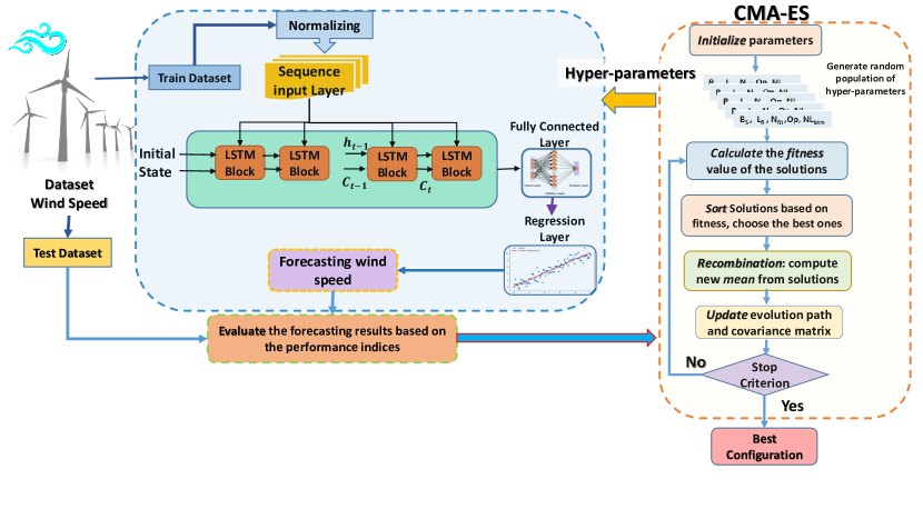
Figure 1: The forecasting framework of the proposed hybrid CMAES-LSTM model.

Figure 1 shows the overall optimization process of our hybrid model.

4 Performance indices of forecasting models

We use five broadly considered performance to assess the forecasting performance: the mean square error (MSE), the root mean square error (RMSE), mean absolute error (MAE), the mean absolute percentage error (MAPE) and the Pearson correlation coefficient (R) [41]. The equations of MAE, RMSE, MAPE and R are represented as follows :

$$MAE=\frac{1}{N}\sum_{i=1}^{N}|f_{p}(i)-f_{o}(i)|$$ (10)

$$RMSE=\sqrt{\frac{1}{N}\sum_{i=1}^{N}(f_{p}(i)-f_{o}(i))^{2}}$$ (11)

$$MAPE=\frac{1}{N}\sum_{i=1}^{N}\frac{(f_{p}(i)-f_{o}(i))}{f_{o}(i)}\times 100\%$$ (12)

$$R=\frac{\frac{1}{N}\sum_{i=1}^{N}(f_{p}(i)-\overline{f}_{p})(f_{o}(i)-\overline{f}_{o})}{\sqrt{\frac{1}{N}\sum_{i=1}^{N}(f_{p}(i)-\overline{f}_{p})^{2}}\times\sqrt{\frac{1}{N}\sum_{i=1}^{N}(f_{o}(i)-\overline{f}_{o})^{2}}}$$ (13)

where $f_{p}(i)$ and $f_{o}(i)$ signify the predicted and observed wind speed values at the $i^{th}$ data point. The total number of observed data points in $N$. In addition, $\overline{f}_{p}$ and $\overline{f}_{o}$ are the average of the projected and observed consequences, respectively. For improving the performance of the predicted model, MSE, RMSE, MAE and MAPE should be minimised, while R needs to be maximized.

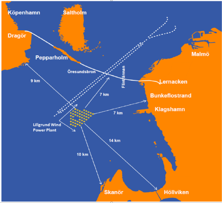
Figure 2: Location of the Lillgrund offshore wind power plant [42].

5 Case Study

In this paper, we use the original wind speed data gathered from a large offshore wind farm called Lillgrund [42] , which is situated in a shallow area of Oresund, located 7 km off the coast of Sweden and 7 km south from the Oresund Bridge connecting Sweden and Denmark (see Figure 2). The mean wind speed is around 8,5 m/s at hub height. This wind, together with the low water depth of 4 to 8 (m), makes the installation of wind turbines economically feasible. The Lillgrund offshore wind farm consists of 48 wind turbines, each rated at 2.3 (MW), resulting in a total wind power plant potential of 110 (MW) [43]. A SCADA collects wind power plant information at a 10-minute interval [44]. The wind power system also includes an offshore substation, an onshore substation and a 130 (kV) sea and land cable for connecting to shore.

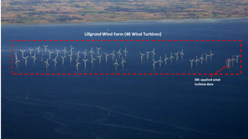
Figure 3: Lillgrund offshore wind farm in Baltic Sea and the wind turbine position is showed with red cycle which is applied for collecting the real wind speed data [42].

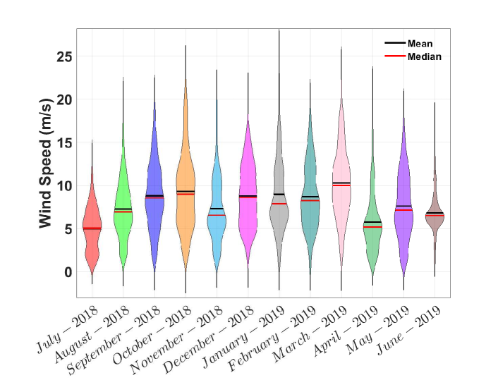
Figure 4: the distribution and frequency of the wind speed data in Lillgrund Wind coastal site per 12 months.

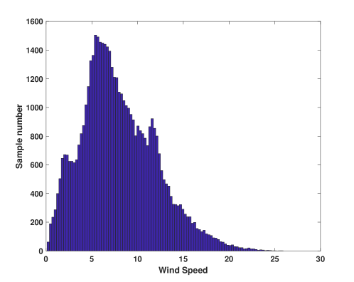
Figure 5: Total distribution and frequency of the wind speed in Lillgrund Wind coastal site .

The wind speed data collected from the Lillgrund wind farm (D3 wind turbine position can be seen in Figure 3) consists of the period from July 2018 to July 2019 at a ten-minute resolution. Figures 4 and 5 show the distribution and frequency of the recorded wind speed in Lillgrund Wind farm during these 12 months. The distribution and frequency of the wind speed is strongly anisotropic[45].

Figure 6 shows that the dominating wind direction is south-west, and a secondary prevailing direction is south-east. However, there are also occasional North-west winds and sporadic north-east storms.

We use two horizons to predict wind speeds: ten minutes and one hour. The wind speed data are randomly divided into three sets using blocks of indices including 80% of the data is used as the training set, and the other 20% is allocated as the test (10%) and validation (10%) set. And also We apply k-fold cross-validation for training the LSTM network in order to predict the time series data.

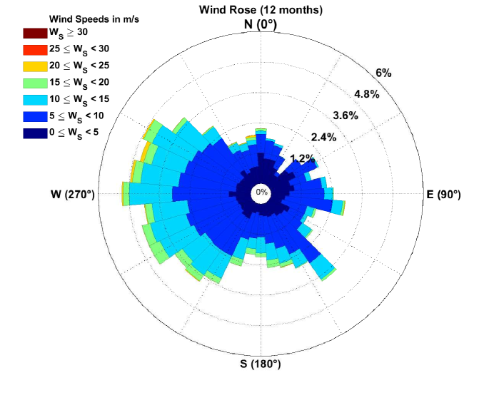
Figure 6: Wind rose: the speed and directional distribution of wind for the Lillgrund Wind coastal site. The dataset for generating this graph was obtained from [42]

6 Experiments and analysis

For assessing the performance of the proposed CMAES-LSTM hybrid model, we compare its performance with four well-known conventional forecasting techniques including FNN, ANFIS, PNN, NAR and one DNN forecasting model (the grid-search tuned LSTM network).

In the first step of this study, a grid search algorithm is used to explore the search space of the hyper-parameters’ impact on LSTM Network performance. Conventionally, tuning hyper-parameters is done by hand and requires skilled practitioners[46]. Here the grid search is limited to tuning learning rate and batch size. Other parameters are fixed to allow the search to complete in reasonable time.

Table 1 shows the final hyper-parameters of the models. We repeat each experiment ten times to ensure to allow for a reasonable sampling of each method’s performance.

Figure 7 demonstrates the forecasting results of tuning both batch size and learning rate in LSTM model performance for the two time-interval prediction dataset. According to the observations, the minimum learning error occurs where the learning rate is between $10^{-4}$ and $10^{-2}$. The optimal size of batches is highly dependent on the selected learning rate values.

Figure 8 shows the correlation between the original wind speed data with predicted ones for the ten-minute and one-hour forecast period.

The average errors of the testing model obtained by the best configuration of the grid-search tuned LSTM model are shown in Figure 8.

One of the best forecasting models is adaptive neuro-fuzzy inference system (ANFIS) [35]. For modelling the wind speed by proper membership functions, five Gaussian membership functions are defined to cover all range of the wind speed dataset (Figure 9). The performance of ANFIS is represented in Figure 10. We can see that the ANFIS estimation results are competitive.

Figure 11 shows the results of the four performance indices applied in this work for short term wind speed forecasting (ten-minute ahead) received by five other models and the proposed hybrid model. Concerning this experiment, the hybrid evolutionary model can outperform the other five competitors for short term wind speed forecasting with the minimum value of RMSE as $0.695(m/s)$, MAE as $0.495(m/s)$, and MAPE as $8.2\%$ as well as the highest rate of R as $98.7$.

Tables 2 and 3 summarise the statistical forecasting results for ten-minute and one-hour intervals. For both time intervals, our CMAES-LSTM can accomplish better forecasting outcomes than other applied models.

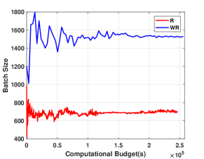
(a)

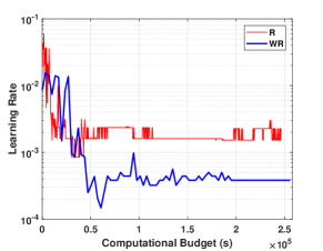
(b)

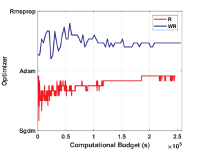
(c)

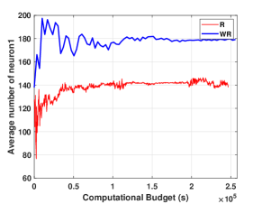
(d)

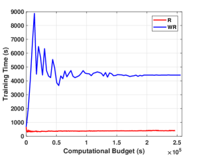
(e)

Figure 13: Comparison of CMAES performance for optimising the Hyper-parameters of the applied LSTM network for forecasting the short-term wind speed (10-minute ahead). For evaluating the performance of the LSTM model, two approaches are employed: applying a penalty for time consuming training runtime experiment (R) and without this penalty (WR). (a) the average of Batch Size (b) the average of learning rate, (c) Optimiser (Sgdm, Adam and Rmsprop), (d) average number of neurons in the first LSTM layer, (e) average of training runtime

In addition, in Figure 12 can be seen that CMAES-LSTM stands the first rank based on the Friedman statistic test with p-values less than $0.0001$, which signifies that the proposed forecasting method considerably performs better than other models. For evaluating the impact of the penalty factor on the Hybrid forecasting model performance, Figure 13 shows the comparison convergence of the hyper-parameters tuning process within (WR) and without (R) applying the penalty factor of the training runtime. Interestingly, both cases are converged to the same learning rate at $10^{-3}$; however, in other parameters, the optimization results are different. It is noted that the whole allocated budget for both cases is the same, but the performance of CMAES-LSTM model with a training runtime penalty is better than another strategy.

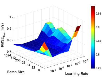
(a)

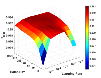
(b)

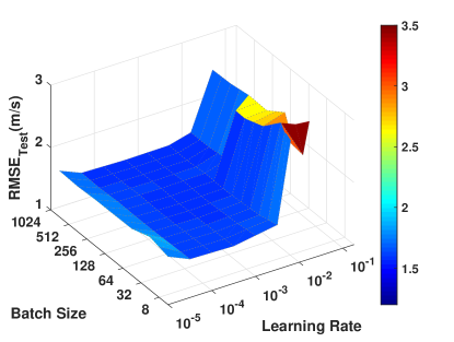
(c)

(d)

Figure 7: Hyper-parameters tuning of the applied LSTM network for forecasting the short-term wind speed .(a) the average of RMSE test-set (ten-minute ahead) (b) the average of R-value test-set (ten-minute ahead), (c) the average of RMSE test-set (one-hour ahead) (d) the average of R-value test-set (one-hour ahead)

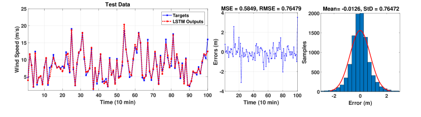
(a)

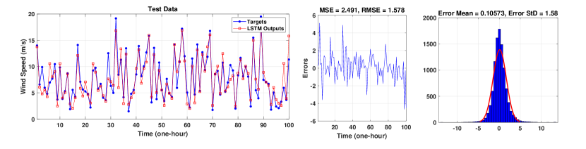
(b)

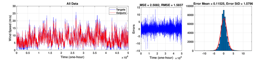
(c)

Figure 8: The wind speed forecasting results achieved by LSTM network with the best tuned hyper-parameters on (a) ten-minute ahead, (b) one-hour ahead (test data-set) and (c) one-hour ahead (all data-set)

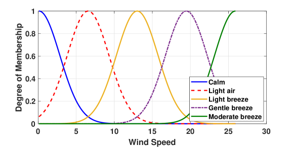
Figure 9: fuzzy memberships applied for modelling the wind speed in ANFIS.

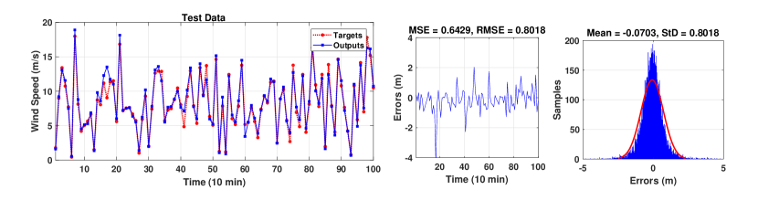
Figure 10: The wind speed forecasting results achieved by ANFIS network with the best tuned hyper-parameters on ten-minute ahead

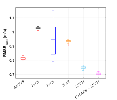
(a)

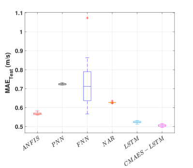
(b)

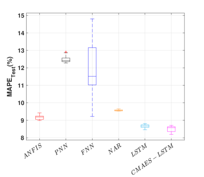
(c)

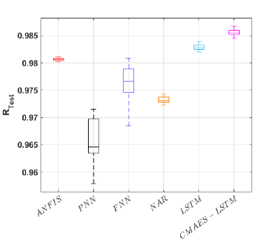
(d)

Figure 11: The performance of different forecasting models results of ten-minute ahead (a) RMSE (b) MAE (c) MAPE and (d) R-value .

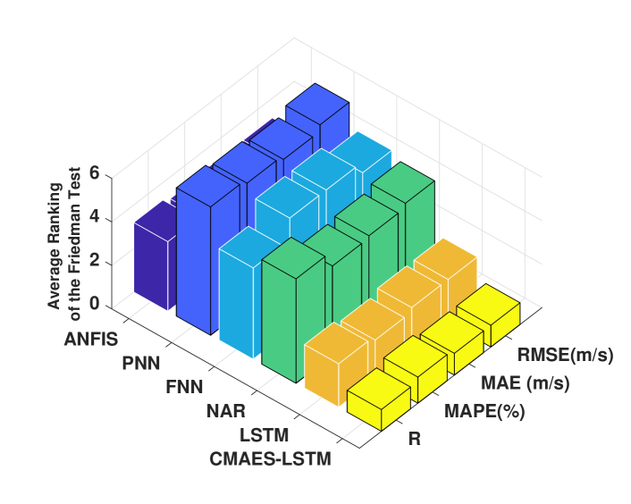
Figure 12: Average ranking of the Friedman test for performance indices statistical tests achieved by various applied forecasting models (ten-minute ahead).

Table 2: Performance indices of forecasting outcomes achieved by different models on case ten-minute ahead.

4		MSE(m/s)		RMSE(m/s)		MAE(m/s)		MAPE(%)		R
Model		Train	Test	Train	Test	Train	Test	Train	Test	Train	Test
	Mean	6.60E-01	6.64E-01	8.13E-01	8.15E-01	5.69E-01	5.69E-01	9.19E+00	9.17E+00	9.81E-01	9.81E-01
ANFIS	Min	6.53E-01	6.43E-01	8.08E-01	8.02E-01	5.66E-01	5.61E-01	9.12E+00	8.99E+00	9.80E-01	9.80E-01
	Max	6.71E-01	6.96E-01	8.19E-01	8.34E-01	5.75E-01	5.82E-01	9.27E+00	9.42E+00	9.81E-01	9.81E-01
	Std	4.58E-03	1.55E-02	2.82E-03	9.47E-03	2.49E-03	7.07E-03	4.83E-02	1.39E-01	1.99E-04	3.23E-04
4	Mean	1.06E+00	1.06E+00	1.03E+00	1.03E+00	7.25E-01	7.24E-01	1.25E+01	1.25E+01	9.67E-01	9.67E-01
PNN	Min	1.05E+00	1.02E+00	1.03E+00	1.01E+00	7.22E-01	7.19E-01	1.24E+01	1.23E+01	9.66E-01	9.66E-01
	Max	1.08E+00	1.08E+00	1.04E+00	1.04E+00	7.28E-01	7.32E-01	1.26E+01	1.29E+01	9.69E-01	9.70E-01
	Std	7.64E-03	1.78E-02	3.70E-03	8.70E-03	2.04E-03	4.69E-03	7.40E-02	2.22E-01	2.40E-03	3.10E-03
4	Mean	9.73E-01	9.56E-01	9.78E-01	9.68E-01	7.24E-01	7.19E-01	1.22E+01	1.22E+01	9.76E-01	9.77E-01
FFNN	Min	6.26E-01	6.28E-01	7.91E-01	7.92E-01	5.61E-01	5.61E-01	9.11E+00	9.22E+00	9.68E-01	9.68E-01
	Max	1.25E+00	1.24E+00	1.12E+00	1.11E+00	8.56E-01	8.53E-01	1.45E+01	1.44E+01	9.81E-01	9.82E-01
	Std	2.77E-01	2.84E-01	1.38E-01	1.42E-01	1.32E-01	1.34E-01	2.30E+00	2.24E+00	5.04E-03	4.84E-03
4	Mean	8.69E-01	8.69E-01	9.32E-01	9.32E-01	6.27E-01	6.28E-01	9.57E+00	9.51E+00	9.73E-01	9.73E-01
NAR	Min	8.56E-01	8.47E-01	9.25E-01	9.20E-01	6.24E-01	6.21E-01	9.54E+00	9.30E+00	9.73E-01	9.72E-01
	Max	8.78E-01	8.87E-01	9.37E-01	9.42E-01	6.29E-01	6.32E-01	9.61E+00	9.60E+00	9.74E-01	9.74E-01
	Std	8.83E-03	1.87E-02	4.73E-03	9.98E-03	2.65E-03	4.44E-03	3.66E-02	8.70E-02	3.39E-04	5.43E-04
4	Mean	5.64E-01	5.60E-01	7.51E-01	7.48E-01	5.23E-01	5.24E-01	8.65E+00	8.66E+00	9.83E-01	9.83E-01
LSTM	Min	5.55E-01	5.31E-01	7.45E-01	7.29E-01	5.19E-01	5.13E-01	8.50E+00	8.46E+00	9.83E-01	9.82E-01
	Max	5.70E-01	5.76E-01	7.55E-01	7.59E-01	5.26E-01	5.29E-01	8.74E+00	8.77E+00	9.83E-01	9.83E-01
	Std	5.35E-03	1.61E-02	3.56E-03	1.08E-02	2.64E-03	5.60E-03	8.93E-02	1.10E-01	1.42E-04	5.48E-04
4	Mean	5.59E-01	5.00E-01	7.61E-01	7.27E-01	5.20E-01	5.07E-01	8.70E+00	8.57E+00	9.83E-01	9.85E-01
CMAES-LSTM	Min	5.46E-01	4.83E-01	7.39E-01	7.19E-01	5.12E-01	4.95E-01	8.58E+00	8.20E+00	9.83E-01	9.84E-01
	Max	5.65E-01	5.22E-01	7.52E-01	7.30E-01	5.25E-01	5.16E-01	8.76E+00	8.71E+00	9.84E-01	9.87E-01
	Std	4.45E-03	1.41E-02	3.56E-03	1.28E-02	3.64E-03	7.60E-03	5.93E-02	1.60E-01	4.42E-04	2.48E-04
4

Table 3: Performance indices of forecasting outcomes achieved by different models on the case of one-hour ahead.

4		MSE(m/s)		RMSE(m/s)		MAE(m/s)		MAPE(%)		R
Model		Train	Test	Train	Test	Train	Test	Train	Test	Train	Test
ANFIS	Mean	2.60E+00	2.59E+00	1.61E+00	1.61E+00	1.16E+00	1.16E+00	2.05E+01	2.05E+01	9.19E-01	9.19E-01
	Min	2.58E+00	2.49E+00	1.61E+00	1.58E+00	1.16E+00	1.15E+00	2.04E+01	2.02E+01	9.18E-01	9.16E-01
	Max	2.62E+00	2.66E+00	1.62E+00	1.63E+00	1.17E+00	1.17E+00	2.06E+01	2.08E+01	9.20E-01	9.21E-01
	Std	1.55E-02	6.62E-02	4.80E-03	2.05E-02	2.54E-03	1.09E-02	7.18E-02	2.59E-01	4.99E-04	1.94E-03
4 PNN	Mean	3.93E+00	3.91E+00	1.98E+00	1.98E+00	1.48E+00	1.48E+00	3.01E+01	3.03E+01	8.73E-01	8.73E-01
	Min	3.90E+00	3.85E+00	1.97E+00	1.96E+00	1.48E+00	1.47E+00	2.98E+01	2.97E+01	8.70E-01	8.72E-01
	Max	3.95E+00	3.96E+00	1.99E+00	1.99E+00	1.49E+00	1.49E+00	3.03E+01	3.06E+01	8.75E-01	8.74E-01
	Std	2.02E-02	4.72E-02	5.10E-03	1.19E-02	3.63E-03	8.71E-03	1.52E-01	3.80E-01	1.90E-03	9.00E-04
4 FFNN	Mean	3.39E+00	3.41E+00	1.82E+00	1.82E+00	1.36E+00	1.36E+00	2.61E+01	2.62E+01	9.15E-01	8.95E-01
	Min	2.65E+00	2.59E+00	1.63E+00	1.61E+00	1.17E+00	1.14E+00	2.04E+01	1.97E+01	9.05E-01	8.95E-01
	Max	4.65E+00	4.66E+00	2.12E+00	2.12E+00	1.61E+00	1.62E+00	3.20E+01	3.24E+01	9.20E-01	8.99E-01
	Std	1.26E+00	1.26E+00	2.97E-01	2.96E-01	2.56E-01	2.59E-01	5.99E+00	6.22E+00	5.03E-03	4.70E-03
4 NAR	Mean	3.55E+00	3.57E+00	1.88E+00	1.89E+00	1.44E+00	1.44E+00	3.49E+01	3.59E+01	8.95E-01	8.95E-01
	Min	3.49E+00	3.46E+00	1.87E+00	1.86E+00	1.43E+00	1.41E+00	3.46E+01	3.46E+01	8.95E-01	8.93E-01
	Max	3.59E+00	3.65E+00	1.90E+00	1.91E+00	1.45E+00	1.46E+00	3.52E+01	3.67E+01	8.96E-01	8.97E-01
	Std	3.83E-02	8.08E-02	1.01E-02	2.14E-02	8.42E-03	1.89E-02	2.20E-01	8.66E-01	5.59E-04	1.49E-03
4 LSTM	Mean	2.50E+00	2.49E+00	1.58E+00	1.58E+00	1.15E+00	1.15E+00	2.27E+01	2.23E+01	9.21E-01	9.22E-01
	Min	2.47E+00	2.43E+00	1.57E+00	1.56E+00	1.15E+00	1.14E+00	2.23E+01	2.15E+01	9.20E-01	9.18E-01
	Max	2.52E+00	2.54E+00	1.59E+00	1.59E+00	1.15E+00	1.16E+00	2.29E+01	2.28E+01	9.22E-01	9.24E-01
	Std	1.80E-02	5.18E-02	5.68E-03	1.64E-02	4.23E-03	1.05E-02	2.50E-01	5.43E-01	5.70E-04	2.29E-03
4 CMAES-LSTM	Mean	2.46E+00	2.46E+00	1.57E+00	1.57E+00	1.14E+00	1.14E+00	2.15E+01	2.18E+01	9.30E-01	9.28E-01
	Min	2.44E+00	2.40E+00	1.56E+00	1.55E+00	1.14E+00	1.13E+00	2.11E+01	2.13E+01	9.30E-01	9.25E-01
	Max	2.48E+00	2.51E+00	1.57E+00	1.58E+00	1.14E+00	1.15E+00	2.18E+01	2.22E+01	9.31E-01	9.31E-01
	Std	1.59E-02	5.49E-02	5.02E-03	1.74E-02	3.92E-03	9.00E-03	3.65E-01	4.19E-01	6.42E-04	2.63E-03
4

7 Conclusions

Wind speed forecasting plays an essential role in the wind energy industry. In this paper, we introduce a hybrid evolutionary deep learning approach (CMAES-LSTM) to acquire highly accurate and more stationary wind speed forecasting results. For tuning the LSTM network hyper-parameters, we propose two different techniques, a grid search and a well-known evolutionary method (CMA-ES). We evaluated the effectiveness of our approach we use data from the Lillgrund offshore wind farm and we use 10-minute and 1-hour time horizons.

Our experiments show that our approach outperforms others using all five performance indices, and that the performance difference is statistically significant.

In the future, we are going to develop the proposed hybrid model by applying a decomposition approach to divide the time series wind speed data to some sub-groups which have more interrelated features. Then each sub-group is absorbed by one independent hybrid method to learn the nonlinear model of wind speed. Another future plan can be further investigations to compare the efficiency of different hybrid evolutionary algorithms and deep learning model based on the nonlinear combined mechanism.

References

- [1] M Majidi Nezhad, D Groppi, P Marzialetti, L Fusilli, G Laneve, F Cumo, and D Astiaso Garcia. Wind energy potential analysis using sentinel-1 satellite: A review and a case study on mediterranean islands. Renewable and Sustainable Energy Reviews, 109:499–513, 2019.
- [2] M Majidi Nezhad, D Groppi, F Rosa, G Piras, F Cumo, and D Astiaso Garcia. Nearshore wave energy converters comparison and mediterranean small island grid integration. Sustainable Energy Technologies and Assessments, 30:68–76, 2018.
- [3] Jeff Lerner, Michael Grundmeyer, and Matt Garvert. The importance of wind forecasting. Renewable Energy Focus, 10(2):64–66, 2009.
- [4] Vikas Khare, Savita Nema, and Prashant Baredar. Solar–wind hybrid renewable energy system: A review. Renewable and Sustainable Energy Reviews, 58:23–33, 2016.
- [5] Jürgen Schmidhuber and Sepp Hochreiter. Long short-term memory. Neural Comput, 9(8):1735–1780, 1997.
- [6] Nikolaus Hansen and Stefan Kern. Evaluating the cma evolution strategy on multimodal test functions. In International Conference on Parallel Problem Solving from Nature, pages 282–291. Springer, 2004.
- [7] Ya-Lan Hu and Liang Chen. A nonlinear hybrid wind speed forecasting model using lstm network, hysteretic elm and differential evolution algorithm. Energy conversion and management, 173:123–142, 2018.
- [8] Guoliang Luo, Erli Dan, Xiaochun Zhang, and Yiwei Guo. Why the wind curtailment of northwest china remains high. Sustainability, 10(2):570, 2018.
- [9] Kurian J Vachaparambil, Eric Aby Philips, Karan Issar, Vaidehi Parab, Divya Bahadur, and Sat Gosh. Optimal siting considerations for proposed and extant wind farms in india. Energy Procedia, 52:48–58, 2014.
- [10] US Fish, Wildlife Service, et al. Biological opinion on the alta east wind project, kern county, california.(3031 (p), caca-052537, cad000. 06)(8-8-13-f-19). memorandum to supervisory projects manager. Renewable Energy, 8, 2013.
- [11] Vinodh K Natarajan and Jebagnanam Cyril Kanmony. Sustainability in india through wind: a case study of muppandal wind farm in india. International Journal of Green Economics, 8(1):19–36, 2014.
- [12] Shiwei Xia, KW Chan, Xiao Luo, Siqi Bu, Zhaohao Ding, and Bin Zhou. Optimal sizing of energy storage system and its cost-benefit analysis for power grid planning with intermittent wind generation. Renewable energy, 122:472–486, 2018.
- [13] Hüseyin Akçay and Tansu Filik. Short-term wind speed forecasting by spectral analysis from long-term observations with missing values. Applied energy, 191:653–662, 2017.
- [14] Ergin Erdem and Jing Shi. Arma based approaches for forecasting the tuple of wind speed and direction. Applied Energy, 88(4):1405–1414, 2011.
- [15] Chuanjin Yu, Yongle Li, Huoyue Xiang, and Mingjin Zhang. Data mining-assisted short-term wind speed forecasting by wavelet packet decomposition and elman neural network. Journal of Wind Engineering and Industrial Aerodynamics, 175:136–143, 2018.
- [16] Abdullah Gani, Kasra Mohammadi, Shahaboddin Shamshirband, Torki A Altameem, Dalibor Petković, and Sudheer Ch. A combined method to estimate wind speed distribution based on integrating the support vector machine with firefly algorithm. Environmental Progress & Sustainable Energy, 35(3):867–875, 2016.
- [17] Chuanjin Yu, Yongle Li, and Mingjin Zhang. An improved wavelet transform using singular spectrum analysis for wind speed forecasting based on elman neural network. Energy Conversion and Management, 148:895–904, 2017.
- [18] Ladislav Zjavka. Wind speed forecast correction models using polynomial neural networks. Renewable Energy, 83:998–1006, 2015.
- [19] Hasan Masrur, Meas Nimol, Mohammad Faisal, and Sk Md Golam Mostafa. Short term wind speed forecasting using artificial neural network: A case study. In 2016 International Conference on Innovations in Science, Engineering and Technology (ICISET), pages 1–5. IEEE, 2016.
- [20] Shouxiang Wang, Na Zhang, Lei Wu, and Yamin Wang. Wind speed forecasting based on the hybrid ensemble empirical mode decomposition and ga-bp neural network method. Renewable Energy, 94:629–636, 2016.
- [21] Qinghua Hu, Rujia Zhang, and Yucan Zhou. Transfer learning for short-term wind speed prediction with deep neural networks. Renewable Energy, 85:83–95, 2016.
- [22] HZ Wang, GB Wang, GQ Li, JC Peng, and YT Liu. Deep belief network based deterministic and probabilistic wind speed forecasting approach. Applied Energy, 182:80–93, 2016.
- [23] Hui Liu, Xi-wei Mi, and Yan-fei Li. Wind speed forecasting method based on deep learning strategy using empirical wavelet transform, long short term memory neural network and elman neural network. Energy conversion and management, 156:498–514, 2018.
- [24] Hui Liu, Xiwei Mi, and Yanfei Li. Smart multi-step deep learning model for wind speed forecasting based on variational mode decomposition, singular spectrum analysis, lstm network and elm. Energy Conversion and Management, 159:54–64, 2018.
- [25] Jie Chen, Guo-Qiang Zeng, Wuneng Zhou, Wei Du, and Kang-Di Lu. Wind speed forecasting using nonlinear-learning ensemble of deep learning time series prediction and extremal optimization. Energy conversion and management, 165:681–695, 2018.
- [26] Wenyu Zhang, Jujie Wang, Jianzhou Wang, Zengbao Zhao, and Meng Tian. Short-term wind speed forecasting based on a hybrid model. Applied Soft Computing, 13(7):3225–3233, 2013.
- [27] Mahdi Khodayar and Jianhui Wang. Spatio-temporal graph deep neural network for short-term wind speed forecasting. IEEE Transactions on Sustainable Energy, 10(2):670–681, 2018.
- [28] You Lin, Ming Yang, Can Wan, Jianhui Wang, and Yonghua Song. A multi-model combination approach for probabilistic wind power forecasting. IEEE Transactions on Sustainable Energy, 10(1):226–237, 2018.
- [29] Ekaterina Vladislavleva, Tobias Friedrich, Frank Neumann, and Markus Wagner. Predicting the energy output of wind farms based on weather data: Important variables and their correlation. Renewable energy, 50:236–243, 2013.
- [30] Sinvaldo Rodrigues Moreno and Leandro dos Santos Coelho. Wind speed forecasting approach based on singular spectrum analysis and adaptive neuro fuzzy inference system. Renewable energy, 126:736–754, 2018.
- [31] S Belaid and A Mellit. Prediction of daily and mean monthly global solar radiation using support vector machine in an arid climate. Energy Conversion and Management, 118:105–118, 2016.
- [32] Kenneth O Stanley, Jeff Clune, Joel Lehman, and Risto Miikkulainen. Designing neural networks through neuroevolution. Nature Machine Intelligence, 1(1):24–35, 2019.
- [33] Hans-Georg Beyer and Hans-Paul Schwefel. Evolution strategies–a comprehensive introduction. Natural computing, 1(1):3–52, 2002.
- [34] Nikolaus Hansen and Anne Auger. Principled design of continuous stochastic search: From theory to practice. In Theory and principled methods for the design of metaheuristics, pages 145–180. Springer, 2014.
- [35] Hugo Miguel Inácio Pousinho, Víctor Manuel Fernandes Mendes, and João Paulo da Silva Catalão. A hybrid pso–anfis approach for short-term wind power prediction in portugal. Energy Conversion and Management, 52(1):397–402, 2011.
- [36] M Lydia, S Suresh Kumar, A Immanuel Selvakumar, and G Edwin Prem Kumar. Linear and non-linear autoregressive models for short-term wind speed forecasting. Energy Conversion and Management, 112:115–124, 2016.
- [37] Diederik P Kingma and Jimmy Ba. Adam: A method for stochastic optimization. arXiv preprint arXiv:1412.6980, 2014.
- [38] Bahareh Nakisa, Mohammad Naim Rastgoo, Andry Rakotonirainy, Frederic Maire, and Vinod Chandran. Long short term memory hyperparameter optimization for a neural network based emotion recognition framework. IEEE Access, 6:49325–49338, 2018.
- [39] Aowabin Rahman, Vivek Srikumar, and Amanda D Smith. Predicting electricity consumption for commercial and residential buildings using deep recurrent neural networks. Applied energy, 212:372–385, 2018.
- [40] Mehdi Neshat, Ehsan Abbasnejad, Qinfeng Shi, Bradley Alexander, and Markus Wagner. Adaptive neuro-surrogate-based optimisation method for wave energy converters placement optimisation. In International Conference on Neural Information Processing, pages 353–366. Springer, 2019.
- [41] Chu Zhang, Jianzhong Zhou, Chaoshun Li, Wenlong Fu, and Tian Peng. A compound structure of elm based on feature selection and parameter optimization using hybrid backtracking search algorithm for wind speed forecasting. Energy Conversion and Management, 143:360–376, 2017.
- [42] Joakim Jeppsson, Poul Erik Larsen, and Aake Larsson. Technical description lillgrund wind power plant: Lillgrund pilot project, 2008.
- [43] Tuhfe Göçmen and Gregor Giebel. Estimation of turbulence intensity using rotor effective wind speed in lillgrund and horns rev-i offshore wind farms. Renewable Energy, 99:524–532, 2016.
- [44] J.Å. Dahlberg. Assessment of the lillgrund wind farm: Power performance wake effects.
- [45] Tarmo Soomere. Anisotropy of wind and wave regimes in the baltic proper. Journal of Sea Research, 49(4):305–316, 2003.
- [46] Leslie N. Smith. A disciplined approach to neural network hyper-parameters: Part 1 – learning rate, batch size, momentum, and weight decay, 2018.