Lie Bracket Approximation-Based Extremum Seeking with Vanishing Input Oscillations

Abstract

In recent years, an approach to extremum seeking control made it possible to design control vector fields that lead to asymptotic stability of the minimum point provided that the minimum value of the function is known a priori. In this work we aim to relax that assumption. We propose an extremum seeking control law that converges to the minimum point with vanishing control oscillations, without access to the minimum value of the cost function. We provide a numerical example to support our results.

,

1 Introduction

Extremum seeking control is an adaptive control technique that drives the steady-state response of a dynamical system to a neighborhood of the minimum point of a cost function in the absence of direct access to gradient information. For more details, the reader is referred to [1, 14, 19, 21] and the references therein. In this paper, we focus on extremum seeking systems that exploit high amplitude, high frequency, sinusoidal signals. This type of signal is prominently used in motion planning of nonholonomic systems [7, 10, 13], and techniques from averaging theory are typically applied for analysis [11, 12]. The first connection to the motion planning framework appears in the reference [4]. Thenceforth, several authors have contributed to this line of work, e.g. [2, 3, 5, 6, 9, 15, 16, 17, 18, 20].

Traditional extremum seeking [4, 8] suffers from persistent oscillations of the steady state response around the minimum point. A solution was proposed in [16], where the authors extended the averaging techniques in [11] to nonsmooth systems, which enabled analysis for a set of nonsmooth control vector fields with useful properties such as vanishing at minimum points. A different set of nonsmooth control functions was proposed in [20], which allowed asymptotic stability of the minimum point. Later, it was shown in [6] that both sets of control functions proposed in [16, 20] belong to a unifying class of generating vector fields. Nevertheless, one of the main assumptions in all these efforts [5, 6, 16, 20] to guarantee asymptotic convergence to the minimum is that the function value at the minimum point is known a priori. This was pointed out explicitly in several locations, for instance in [5, 6].

The contribution of this paper is to provide an extension of the results highlighted so far to the case when the minimum value of the function is unknown. Specifically, we prove asymptotic convergence to the minimum point with bounded amplitude and frequency, for all initial conditions in a subset of the epigraph of the cost function.

2 Main Theorem

Notations: We use bold characters to distinguish vectors and vector valued maps from scalars. Let $D\subset\mathbb{R}^{n}$ be a subset. We denote the set of $k$-times continuously differentiable real-valued functions on $D$ by $C^{k}(D;\mathbb{R})$. We denote by $\bm{e}_{j}$ the $j^{th}$ canonical unit vector in $\mathbb{R}^{n}$. The set of vector fields with regularity $\nu\in\mathbb{N}$ on $\mathbb{R}^{n}$ is denoted by $\Gamma^{\nu}(\mathbb{R}^{n})$. The Lie derivative of a function $g\in C^{1}(\mathbb{R}^{n};\mathbb{R})$ along a vector field $\bm{f}\in\Gamma^{\nu}(\mathbb{R}^{n})$ is written as $L_{\bm{f}}\,g(\bm{x})$. The Lie bracket between two vector fields $\bm{f}_{1},\bm{f}_{2}\in\Gamma^{1}(\mathbb{R}^{n})$ is computed as $[\bm{f}_{1},\bm{f}_{2}](\bm{x})=\textbf{J}_{\bm{f}_{2}}(\bm{x})\bm{f}_{1}(\bm{x})-\textbf{J}_{\bm{f}_{1}}(\bm{x})\bm{f}_{2}(\bm{x}),$ where $\textbf{J}_{\bm{f}}(\bm{x})$ is the standard Jacobian of $\bm{f}$ in the $\bm{x}$-coordinates.

Let $D\subset\mathbb{R}^{n}$ be a bounded subset with a nonempty interior. Suppose that $J:D\rightarrow\mathbb{R}$ is a cost function that has the following properties:

Assumption 1.

A1 Assume that $J\in C^{3}(D;\mathbb{R})$ and that there exists a unique point $\bm{x}^{*}\in D$, such that $\tilde{J}(\bm{x})=J(\bm{x})-J^{*}>0~{}\forall\bm{x}\neq\bm{x}^{*}$, where $J^{*}=J(\bm{x}^{*})$ and

$$\kappa_{1}\tilde{J}(\bm{x})^{2-\frac{1}{m}}\leq\lVert\nabla J(\bm{x})\lVert^{2}\leq\kappa_{2}\tilde{J}(\bm{x})^{2-\frac{1}{m}}$$

$$\gamma_{1}\tilde{J}(\bm{x})^{1-\frac{1}{m}}\leq\lVert\nabla^{2}J(\bm{x})\lVert\leq\gamma_{2}\tilde{J}(\bm{x})^{1-\frac{1}{m}}$$

where $\kappa_{i},\gamma_{i}>0$ and $m\geq 1$.

Next, define the epigraph and strict epigraph of $J$

$$\text{epi}(J) =\big{\{}(\bm{x},z)\in D\times\mathbb{R}\big{|}J(\bm{x})-z\leq 0\big{\}}$$

$$\text{epi}_{S}(J) =\big{\{}(\bm{x},z)\in D\times\mathbb{R}\big{|}J(\bm{x})-z<0\big{\}},$$

Let $\bm{\theta}=(\bm{x},z)\in\text{epi}_{S}(J)$, and define the functions $g_{i}:\text{epi}_{S}(J)\rightarrow\mathbb{R},~{}i\in\{1,2,3\}$

$$g_{1}(\bm{\theta}) =\tilde{J}(\bm{x})-J_{0},\quad g_{2}(\bm{\theta})=z-J^{*}-z_{0}$$ (1)

$$g_{3}(\bm{\theta}) =\frac{\tanh(\tilde{J}(\bm{x})^{2-\frac{1}{m}})}{z-J(\bm{x})}-y_{0}$$

where $J_{0},y_{0},z_{0}$ are positive constants. Let $\epsilon>0$ and define the domains

$$\Delta_{0} =\big{\{}\bm{\theta}\in\text{epi}_{S}(J)\big{|}g_{i}(\bm{\theta})\leq 0,~{}\forall i\in\{1,2,3\}\big{\}}$$

$$\Delta_{\epsilon} =\big{\{}\bm{\theta}\in\text{epi}_{S}(J)\big{|}g_{i}(\bm{\theta})\leq\epsilon,~{}\forall i\in\{1,2,3\}\big{\}}$$

Let $\Lambda$ denote the set of all ordered pairs $(j,s)$, where $j\in\{1,...,n\},s\in\{1,2\}$. Then, consider the dynamical system

$$\dot{\bm{\theta}} =\bm{f}_{0}(\bm{\theta})+\sum_{\lambda\in\Lambda}\bm{f}_{\lambda}(\bm{\theta})u_{\lambda}(t)$$ (2)

$$\bm{f}_{0}(\bm{\theta}) =-(z-J(\bm{x}))~{}\bm{e}_{n+1}$$

$$\bm{f}_{j,s}(\bm{\theta}) =F_{s}(z-J(\bm{x}))~{}\bm{e}_{j}$$

and the functions $u_{j,1},u_{j,2}$ (the dithers) are given by

$$u_{j,1}(t) =2\sqrt{\pi\omega_{j}\omega}\sin(2\pi\omega_{j}\omega t)$$ (3)

$$u_{j,2}(t) =2\sqrt{\pi\omega_{j}\omega}\cos(2\pi\omega_{j}\omega t)$$

where $\omega\in(0,\infty),~{}\omega_{j}\in\mathbb{N},~{}\forall j\in\{1,2,...,n\}$, and the functions $F_{1}(\cdot),F_{2}(\cdot)$ are given by:

$$F_{1}(y) =\sqrt{y}\sin{(\log(y))}$$ (4)

$$F_{2}(y) =\sqrt{y}\cos{(\log(y))}$$

Note that other choices for $F_{s}(\cdot)$ are possible [6]. Also note that the second equation in system (2) is similar to the approach in [17].

Theorem 2.

main_thm Suppose that the function $J$ satisfies A1, and consider the system defined by (2), (3) and (4). Fix a choice for the collection of frequencies $~{}\omega_{j}\in\mathbb{N},~{}\forall j\in\{1,2,...,n\}$ such that $\forall i\neq j$, $\omega_{i}\neq\omega_{j}$. Then, $\exists\omega^{*}\in(0,\infty)$ such that $\forall\omega\in(\omega^{*},\infty),~{}\forall\bm{\theta}(0)\in\Delta_{0}$ we have:

1. $\bm{\theta}(t)\in\Delta_{\epsilon},\forall t\in[0,\infty)$,

2. $\bm{\theta}(t)\rightarrow(\bm{x}^{*},J^{*})\text{ as }~{}t\rightarrow\infty$.

The proof is in appendix B. Note that we outline a procedure to estimate a sufficiently high frequency $\omega^{*}$ in lem2,lem3.

Remark 3.

Since $J(x(0))$ is available via measurement, it is always possible to place $z(0)$, which is an internal state of the controller, such that the initial condition strictly lies in $\Delta_{0}$. We emphasize that this does not require additional information other than online measurement of the function value.

3 Numerical Simulations

Example 4.

Let $\bm{x}\in\mathbb{R}^{2}$, and consider the dynamical system

$$\dot{\bm{x}} =\textbf{A}(t)(\bm{x}-\bm{x}^{*})+\textbf{B}\bm{u}$$ (5)

$$J(\bm{x},t) =\frac{3}{2}\lVert\bm{x}-\bm{x}^{*}\lVert^{2}+5(1+\exp(-t))$$

where $\bm{u}\in\mathbb{R}^{2}$ is the control input, $\bm{x}^{*}=(1,-1)$, and

$$\textbf{A}(t)=\begin{bmatrix}\cos(t)^{2}&\sin(t)^{2}\\ -\sin(t)^{2}&\cos(t)^{2}\end{bmatrix},\quad\textbf{B}=\begin{bmatrix}1&1\\ -1&1\end{bmatrix}$$

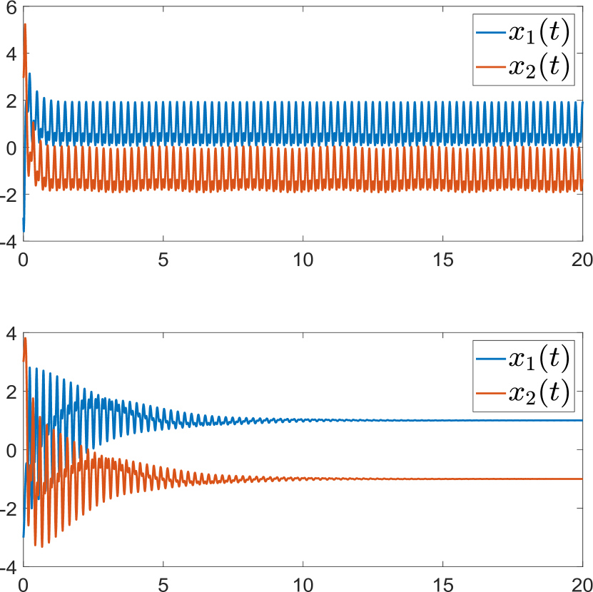
Figure 1: (left): Illustration of $\Delta_{0},\Delta_{\epsilon}$ and sample trajectories, (right): Numerical results of Example 3.1 for the approach in [6] (top), and our approach (bottom)

The numerical results for the proposed control law are shown in Fig.(1), where we used the initial conditions $\bm{x}(0)=(-3,3),~{}z(0)=J(\bm{x}(0))+3=61,$ and the frequency parameters $\omega=4,~{}\omega_{1}=1,\omega_{2}=2$.

Remark 5.

We remark that the proposed method can tolerate bounded monotonic decrease of the minimum value of the function as demonstrated in the provided example. However, we emphasize that it does not tolerate general time-dependent variations of the cost function in the current formulation. This is due to the nature of the dynamic upper bound on the cost function (i.e. $z(t)$).

4 Conclusion and Future work

In this brief note, we propose an extension to extremum seeking control via Lie bracket approximations that allows asymptotic convergence to the minimum point for a cost function in the absence of information on its minimum value. The proposed control law leads to bounded control signals that vanish as the system converges to the minimum point, and bounded frequency of oscillation. We also a provide a procedure to obtain an estimate on the required frequency. Numerical simulations show that similar results may hold for the case of a dynamic cost function under appropriate assumptions on the dynamics.

Appendix A Preliminary Results

Consider the Initial Value Problem (IVP)

$$\dot{\bm{\zeta}}(t)=\bm{f}_{0}(\bm{\zeta}(t))+\sum\limits_{\lambda\in\Lambda}\bm{f}_{\lambda}(\bm{\zeta}(t))~{}u_{\lambda}(t),\quad\bm{\zeta}(0)\in\Xi_{0}$$ (6)

where $\Xi_{0}\subset\Xi\subset\mathbb{R}^{n}$, $\Lambda$ is the set of all ordered pairs $(j,s),j\in\{1,2,...,n\},s\in\{1,2\}$, $\bm{f}_{0},\bm{f}_{\lambda}\in\Gamma^{2}(\Xi)$ and the dither signals $u_{\lambda}(\cdot)$ are defined by Eq. (3)

Lemma 6.

lem1[4, 11, 17] Let $g\in C^{3}(\Xi;\mathbb{R})$. Then, for every solution $\bm{\zeta}:I\rightarrow\Xi$ of (6), the function $g\circ\bm{\zeta}:I\rightarrow\mathbb{R}$ satisfies

$$g(\bm{\zeta}(t))\big{|}_{t_{1}}^{t_{2}}=R^{g}_{1}(\bm{\zeta}(t),t)\big{|}_{t_{1}}^{t_{2}}+\int\limits_{t_{1}}^{t_{2}}\big{(}F^{g}(\bm{\zeta}(t))+R^{g}_{2}(\bm{\zeta}(t),t)\big{)}dt$$

where $I$ is the interval of existence and uniqueness of $\bm{\zeta}(\cdot)$, $t_{1},t_{2}\in I,t_{2}>t_{1}$, and

$$F^{g}(\bm{\zeta}) =L_{\bm{f}_{0}}g(\bm{\zeta})-\sum\limits_{j=1}^{m}L_{[\bm{f}_{j,1},\bm{f}_{j,2}]}g(\bm{\zeta})$$

$$R^{g}_{1}(\bm{\zeta},t) =~{}\sum\limits_{\lambda\in\Lambda}L_{\bm{f}_{\lambda}}g(\bm{\zeta})~{}U_{\lambda}(t)$$

$$-\sum\limits_{\lambda_{1},\lambda_{2}\in\Lambda}L_{\bm{f}_{\lambda_{2}}}L_{\bm{f}_{\lambda_{1}}}g(\bm{\zeta})~{}U_{\lambda_{1},\lambda_{2}}(t)$$

$$R^{g}_{2}(\bm{\zeta},t) =-\sum\limits_{\lambda\in\Lambda}L_{\bm{f}_{0}}L_{\bm{f}_{\lambda}}g(\bm{\zeta})~{}U_{\lambda}(t)$$

$$+\sum\limits_{\lambda_{1},\lambda_{2}\in\Lambda}L_{\bm{f}_{0}}L_{\bm{f}_{\lambda_{2}}}L_{\bm{f}_{\lambda_{1}}}g(\bm{\zeta})~{}U_{\lambda_{1},\lambda_{2}}(t)$$

$$+\sum\limits_{\lambda_{1},\lambda_{2},\lambda_{3}\in\Lambda}L_{\bm{f}_{\lambda_{3}}}L_{\bm{f}_{\lambda_{2}}}L_{\bm{f}_{\lambda_{1}}}g(\bm{\zeta})~{}U_{\lambda_{1},\lambda_{2}}(t)u_{\lambda_{3}}(t)$$

$$U_{\lambda}(t) =\int u_{\lambda}(t)~{}dt$$

$$U_{\lambda_{1},\lambda_{2}}(t) =\int\bigg{(}v_{\lambda_{1},\lambda_{2}}+U_{\lambda_{1}}(t)~{}u_{\lambda_{2}}(t)\bigg{)}d\tau$$

$$v_{\lambda_{1},\lambda_{2}} =\begin{cases}+1&\lambda_{1}=(j,1)\quad\&\quad\lambda_{2}=(j,2)\\ -1&\lambda_{1}=(j,2)\quad\&\quad\lambda_{2}=(j,1)\\ 0&\qquad\quad otherwise\end{cases}$$

Lemma 7.

lem2 Let $\Xi\subseteq\mathbb{R}^{n},g_{i}\in C^{3}(\Xi;\mathbb{R})~{}\forall i\in\{1,2,...,r\}$. Let $\epsilon>0$ and define

$$\Delta_{0} =\big{\{}\bm{\zeta}\in\Xi\big{|}g_{i}(\bm{\zeta})\leq 0,~{}\forall i\in\{1,2,..~{},r\}\big{\}}$$

$$\Delta_{\epsilon} =\big{\{}\bm{\zeta}\in\Xi\big{|}g_{i}(\bm{\zeta})\leq\epsilon,~{}\forall i\in\{1,2,..~{},r\}\big{\}}$$

and the subsets $\Delta^{i}_{\epsilon}=\big{\{}\bm{\zeta}\in\Delta_{\epsilon}\big{|}0\leq g_{i}(\bm{\zeta})\leq\epsilon\big{\}}$. Suppose that $\forall i\in\{1,2,...,r\}$, whenever $\bm{\zeta}\in\Delta^{i}_{\epsilon}$, the following bounds hold

$$\big{\lVert}R^{g_{i}}_{1}(\bm{\zeta},t)\big{\lVert}\leq\frac{c^{g_{i}}_{1}}{\sqrt{\omega}},~{}~{}~{}\big{\lVert}R^{g_{i}}_{2}(\bm{\zeta},t)\big{\lVert}\leq\frac{c^{g_{i}}_{2}}{\sqrt{\omega}},~{}~{}~{}F^{g_{i}}(\bm{\zeta})\leq-b^{g_{i}}$$

$\forall t\in\mathbb{R}$, where $c^{g_{i}}_{1},c^{g_{i}}_{2},b^{g_{i}}>0$ are constants. Then $\exists\omega^{*}\in(0,\infty)$ such that $\forall\omega\in(\omega^{*},\infty),\forall\bm{\zeta}(0)\in\Delta_{0}$ and maximal solution  $\bm{\zeta}:\text{I}\rightarrow\Delta_{\epsilon}$ for the IVP (6), where $0\in\text{I}=(t_{e}^{-},t_{e}^{+})$,

$$\limsup\limits_{\tau\rightarrow t_{e}^{+}}g_{i}(\bm{\zeta}(\tau))<\epsilon,~{}\forall i\in\{1,2,..,r\}$$

Fix $\delta\in(0,\epsilon)$. If $g_{i}(\bm{\zeta}(t))<\delta,\forall t\in[0,t_{e}^{+})$, the proof is complete. If not, then, by continuity of $g_{i}\circ\bm{\zeta}$ and the Intermediate Value Theorem, $\exists t_{1},t_{2}\in I$, $t_{2}>t_{1}\geq 0$, where $g_{i}(\bm{\zeta}(t_{1}))=0,~{}g_{i}(\bm{\zeta}(t_{2}))=\delta$, and $\bm{\zeta}(t)\in\Delta^{i}_{\epsilon},~{}\forall t\in[t_{1},t_{2}]$. Using the bounds on $R^{g_{i}}_{1},R^{g_{i}}_{2},F^{g_{i}}$ and lem1, we get

$$g_{i}(\bm{\zeta}(t_{2}))\leq\cancelto{0}{g_{i}(\bm{\zeta}(t_{1}))}\quad+\;\frac{2c^{g_{i}}_{1}}{\sqrt{\omega}}+\int\limits_{t_{1}}^{t_{2}}\bigg{(}-b^{g_{i}}+\frac{c^{g_{i}}_{2}}{\sqrt{\omega}}\bigg{)}~{}dt$$

We define

$$~{}\omega^{*}=\max\limits_{i\in\{1,2,...,r\}}\Big{\{}\Big{(}\frac{2c_{1}^{g_{i}}}{\delta}\Big{)}^{2},\Big{(}\frac{c_{2}^{g_{i}}}{b^{g_{i}}}\Big{)}^{2}\Big{\}}$$

and observe that $\forall\omega\in(\omega^{*},\infty),\forall i\in\{1,2,...,r\}$, we have

$$g_{i}(\bm{\zeta}(t_{2}))<\delta\implies\limsup\limits_{\tau\rightarrow t_{e}^{+}}g_{i}(\bm{\zeta}(\tau))<\epsilon\qed$$

Note that $\omega^{*}$ in the proof of lem2 gives an estimate of the required frequency of oscillation in terms of the constants $c^{g_{i}}_{1},c^{g_{i}}_{2},b^{g_{i}}$ and a choice of $\delta\in(0,\epsilon)$. Thus, to choose a sufficiently large frequency, one needs to know the constants $c^{g_{i}}_{1},c^{g_{i}}_{2},b^{g_{i}}$. In the next lemma, we outline a procedure to estimate these constants under A1 for the static cost case. In fact, for a general dynamical system, if one can establish these bounds on the remainders, then the conclusions of main_thm hold, as demonstrated by the numerical results provided above.

Lemma 8.

lem3 Consider the system (2) and the functions (1). Then, there exists constants $c_{1}^{g_{i}},c_{2}^{g_{i}}>0$ such that, $\forall\bm{\theta}\in\Delta^{i}_{\epsilon},i\in\{1,2,3\}$ and $\forall t\in\mathbb{R}$:

$$\big{\lVert}R^{g_{i}}_{1}(\bm{\theta},t)\big{\lVert}\leq\frac{c^{g_{i}}_{1}}{\sqrt{\omega}},~{}~{}~{}\big{\lVert}R^{g_{i}}_{2}(\bm{\theta},t)\big{\lVert}\leq\frac{c^{g_{i}}_{2}}{\sqrt{\omega}}$$

Via direct integration, the following bounds can be established

$$\left\lvert U_{\lambda_{1}}(t)\right\lvert\leq\frac{a_{1}}{\sqrt{\omega}},\quad\left\lvert U_{\lambda_{1},\lambda_{2}}(t)\right\lvert\leq\frac{a_{1}}{\omega},$$

$$\quad\quad\left\lvert U_{\lambda_{1},\lambda_{2}}(t)u_{\lambda_{3}}(t)\right\lvert\leq\frac{a_{1}}{\sqrt{\omega}}$$

$\forall\lambda_{1},\lambda_{2},\lambda_{3}\in\Lambda,\forall t\in\mathbb{R}$, where $a_{1}>0$ depends on the choice of the frequencies $\omega_{j}$. Due to space constraints, we only show how to establish a bound on one of the highest order terms in $R^{g_{3}}_{2}(\cdot,\cdot)$. The rest of the bounds can be established following the same approach. Let $y=z-J(\bm{x})$. We compute

$$L_{\bm{f}_{(i,1)}}L_{\bm{f}_{(i,1)}}L_{\bm{f}_{(i,1)}}g_{3}(\bm{\theta})=\partial^{3}_{i}g_{3}(\bm{\theta})F_{1}(y)^{3}-2\partial^{2}_{i}g_{3}(\bm{\theta})$$

$$\times F_{1}^{\prime}(y)F_{1}(y)^{2}\partial_{i}J(\bm{x})-\partial^{2}_{i}g_{3}(\bm{\theta})F_{1}^{\prime}(y)F_{1}(y)^{2}\partial_{i}J(\bm{x})$$

$$+ \partial_{i}g_{3}(\bm{\theta})F_{1}^{\prime\prime}(y)F_{1}(y)^{2}\partial_{i}J(\bm{x})^{2}+\partial_{i}g_{3}(\bm{\theta})F_{1}^{\prime}(y)^{2}$$

$$\times F_{1}(y)\partial_{i}J(\bm{x})^{2}-\partial_{i}g_{3}(\bm{\theta})F_{1}^{\prime}(y)F_{1}(y)^{2}\partial^{2}_{i}J(\bm{x})$$

It can be shown by direct computation that, for $y>0$, we have

$$|F_{1}(y)|\leq \sqrt{y},~{}|F_{1}^{\prime}(y)|\leq\frac{2}{\sqrt{y}},~{}|F_{2}^{\prime\prime}(y)|\leq\frac{2}{y\sqrt{y}}$$

$$\partial_{i}g_{3}(\bm{\theta})= (2-\frac{1}{m})\frac{\tilde{J}(\bm{x})^{1-\frac{1}{m}}\partial_{i}J(\bm{x})}{z-J(x)}\text{sech}(\tilde{J}(\bm{x})^{2-\frac{1}{m}})^{2}$$

$$+ \frac{\tanh(\tilde{J}(\bm{x})^{2-\frac{1}{m}})\partial_{i}J(\bm{x})}{(z-J(x))^{2}}$$

$$|\partial_{i}g_{3}(\bm{\theta})|\leq \frac{2\tilde{J}(\bm{x})^{1-\frac{1}{m}}|\partial_{i}J(\bm{x})|}{|z-J(x)|}+\frac{\tilde{J}(\bm{x})^{2-\frac{1}{m}}|\partial_{i}J(\bm{x})|}{(z-J(x))^{2}}$$

Using A1, we can see that

$$|\partial_{i}J(\bm{x})|\leq\lVert\nabla J(\bm{x})\lVert\leq\sqrt{\kappa_{2}}\tilde{J}(\bm{x})^{1-\frac{1}{2m}}$$

Moreover, we know that

$$\frac{\tanh(J(\bm{x})^{2-\frac{1}{m}})}{z-J(\bm{x})}\leq y_{0}+\epsilon,\quad\forall\bm{\theta}\in\Delta^{3}_{\epsilon}$$

Thus, it holds that

$$|\partial_{i}g_{3}(\bm{\theta})|\leq\sqrt{\kappa_{2}}(y_{0}+\epsilon)\frac{\tilde{J}(\bm{x})^{2-\frac{3}{2m}}}{\tanh(\tilde{J}(\bm{x})^{2-\frac{1}{m}})}(2+\tilde{J}(x))$$

For $\theta\in\Delta^{3}_{\epsilon}$, we have $\tilde{J}(\bm{x})\leq J_{0}$, and $|F^{\prime}(y)F(y)|\leq 2$. Thus, we have:

$$|\partial_{i}g_{3}(\bm{\theta})F^{\prime}(y)F(y)\partial_{i}J(\bm{x})|\leq a_{2}\frac{\tilde{J}(\bm{x})^{2-\frac{1}{m}}}{\tanh(\tilde{J}(\bm{x})^{2-\frac{1}{m}})}$$

where $a_{2}=\kappa_{2}J_{0}^{1-\frac{1}{m}}(y_{0}+\epsilon)(2+J_{0})$. Finally, it can be shown that

$$\frac{\tilde{J}(\bm{x})^{2-\frac{1}{m}}}{\tanh(\tilde{J}(\bm{x})^{2-\frac{1}{m}})}\leq\tilde{J}(\bm{x})^{2-\frac{1}{m}}+1$$

This leads to the bound:

$$|\partial_{i}g_{3}(\bm{\theta})F^{\prime}(y)F(y)\partial_{i}J(\bm{x})|\leq a_{3}$$

where $a_{3}=a_{2}(1+J_{0}^{2-\frac{1}{m}})$. Following a similar approach, it can be shown that all the terms in the Lie derivative are bounded, $|L_{\bm{f}_{(i,1)}}L_{\bm{f}_{(i,1)}}L_{\bm{f}_{(i,1)}}g_{3}(\bm{\theta})|\leq a_{4}$, where $a_{4}>0$ is the sum of all the bounds on the individual terms. Consequently, we have established the bound

$$|L_{\bm{f}_{(i,1)}}L_{\bm{f}_{(i,1)}}L_{\bm{f}_{(i,1)}}g_{3}(\bm{\theta})U_{(i,1),(i,1)}(t)u_{(i,1)}(t)|\leq\frac{a_{5}}{\sqrt{\omega}}$$

$\forall\bm{\theta}\in\Delta^{3}_{\epsilon},\forall t\in\mathbb{R}$, where $a_{5}=a_{1}a_{4}>0$. Following this procedure for each individual term in the remainders will give the explicit bounds on $R^{g_{i}}_{1},R^{g_{i}}_{2},i\in\{1,2,3\}$ in terms of the constants $\kappa_{1},\kappa_{2},\gamma_{1},\gamma_{2},\epsilon,J_{0},y_{0},z_{0},\omega_{j}$.

Appendix B Proof of Main Theorem

Let $J_{0}>0$ be such that the level set

$$\mathcal{L}_{J_{0}}=\big{\{}\bm{x}\in\mathbb{R}^{n}\big{|}\tilde{J}(\bm{x})\leq J_{0}\big{\}}\subset D$$

Fix an $\epsilon>0$, and let

$$y_{0}>\frac{1}{2\kappa_{1}}\big{(}1+\sqrt{1+8\kappa_{1}\epsilon}\big{)},~{}~{}z_{0}>J_{0}+y_{0}$$

The functions $F_{s}(\cdot),s\in\{1,2\}$ are locally Lipschitz in $\Delta_{\epsilon}$. Hence, absolutely continuous maximal solutions of (2) with $\bm{\theta}(0)\in\Delta_{\epsilon}$ exist and are unique. We consider a maximal solution $\bm{\theta}:I\rightarrow\Delta_{\epsilon}$ of (2) with $\bm{\theta}(0)\in\Delta_{0}$ and apply lem1 to the functions $g_{i},~{}i\in\{1,2,3\}$ defined by Eq. (1). The next step is to establish the bounds on $F^{g_{i}},R_{1}^{g_{i}},R_{2}^{g_{i}}$ in lem2 for $g_{i}(\cdot),i\in\{1,2,3\}$. We compute

$$F^{g_{1}}(\bm{\theta}) =-\left\lVert\nabla J(\bm{x})\right\lVert^{2}\quad,\quad F^{g_{2}}(\bm{\theta})=-z+J(\bm{x})$$

$$F^{g_{3}}(\bm{\theta}) =\frac{\eta(\tilde{J}(\bm{x})^{2-\frac{1}{m}})}{(z-J(\bm{x}))}-\frac{\eta(\tilde{J}(\bm{x})^{2-\frac{1}{m}})\left\lVert\nabla J(\bm{x})\right\lVert^{2}}{(z-J(\bm{x}))^{2}}$$

$$-\frac{\left(2-\frac{1}{m}\right)\tilde{J}(\bm{x})^{1-\frac{1}{m}}\eta^{\prime}(\tilde{J}(\bm{x})^{2-\frac{1}{m}})\left\lVert\nabla J(\bm{x})\right\lVert^{2}}{z-J(\bm{x})}$$

where $\eta(y)=\tanh(y)$. We note that in case of $g_{2}$, the remainder terms $R^{g_{2}}_{1},R^{g_{2}}_{2}$ in lem1 identically vanish, and the only remaining term inside the integral is

$$F^{g_{2}}(\bm{\theta})=-z+J(\bm{x})<0,~{}\forall\bm{\theta}\in\text{epi}_{S}(J)$$

We conclude, similar to the proof of lem2, that $g_{2}(\bm{\theta}(t))\leq 0,~{}\forall t\in I,~{}\forall\omega\in(0,\infty)$. Due to A1, we know that $\forall\bm{\theta}\in\Delta^{1}_{\epsilon}$, we have

$$F^{g_{1}}(\bm{\theta})\leq-\kappa_{1}J_{0}^{2-\frac{1}{m}}$$

Furthermore, by definition of $g_{3}(\cdot)$, and thanks to the property that $\tanh(y)\leq y,~{}\forall y\geq 0$ and the choice of $y_{0}$, we have

$$F^{g_{3}}(\bm{\theta})\leq y_{0}+\epsilon-\kappa_{1}y_{0}^{2}<-\epsilon,\quad\forall\bm{\theta}\in\Delta^{3}_{\epsilon}$$

The bounds on the remainders $R^{g_{2}}_{1},R^{g_{2}}_{2}$ can be explicitly computed, as outlined in lem3. We now apply lem2 with the bounds established above to conclude that $\exists\omega^{*}\in(0,\infty)$ such that $\forall\omega\in(\omega^{*},\infty),\forall\bm{\theta}(0)\in\Delta_{0}$ and maximal solution  $\bm{\theta}:\text{I}\rightarrow\Delta_{\epsilon}$, where $0\in\text{I}=(t_{e}^{-},t_{e}^{+})$, we have

$$\limsup\limits_{\tau\rightarrow t_{e}^{+}}g_{i}(\bm{\theta}(\tau))<\epsilon,~{}\forall i\in\{1,2,3\}$$

We note that the only remaining boundary in the definitions of $\Delta_{0},\Delta_{\epsilon}$ is the point $(\bm{x}^{*},J(\bm{x}^{*}))$. Clearly $\dot{z}(t)<0$. Moreover, we have that

$$\dot{z}=-z+J(\bm{x})\geq-z+J(\bm{x}^{*})\implies\tilde{z}(t)\geq\tilde{z}(0)e^{-t}>0$$

where $\tilde{z}(t)=z(t)-J(\bm{x}^{*})$. Thus for any finite $t_{e}^{+}>0$, we have that

$$\lim\limits_{\tau\rightarrow t_{e}^{+}}z(\tau)-J(\bm{x}(\tau))>0$$

This implies that $\forall\omega\in(\omega^{*},\infty)$, maximal solutions that start inside $\Delta_{0}$ do not escape $\Delta_{\epsilon}$ in any finite time, hence $[0,\infty)\subset I$. Moreover, since z(t) is bounded below and strictly decreasing, we have that

$$\lim\limits_{\tau\rightarrow+\infty}z(\tau)-J(\bm{x}(\tau))=0$$

Consequently, we see that due to the definition of $g_{3}(\cdot)$, it must be true that

$$\lim\limits_{\tau\rightarrow+\infty}\eta(\tilde{J}(\bm{x}(\tau))^{2-\frac{1}{m}})=0\implies\lim\bm{x}(\tau)=\bm{x}^{*}$$

Combining all of the above, we conclude that

$$\lim\limits_{\tau\rightarrow+\infty}\bm{\theta}(\tau)=(\bm{x}^{*},J(\bm{x}^{*}))$$

References

• [1] Kartik B Ariyur and Miroslav Krstic. Real-time optimization by extremum-seeking control. John Wiley & Sons, 2003.
• [2] Hans-Bernd Dürr, Miroslav Krstić, Alexander Scheinker, and Christian Ebenbauer. Singularly perturbed lie bracket approximation. IEEE Transactions on Automatic Control, 60(12):3287–3292, 2015.
• [3] Hans-Bernd Dürr, Miroslav Krstić, Alexander Scheinker, and Christian Ebenbauer. Extremum seeking for dynamic maps using lie brackets and singular perturbations. Automatica, 83:91–99, 2017.
• [4] Hans-Bernd Dürr, Milos S. Stankovic, Christian Ebenbauer, and Karl Henrik Johansson. Lie bracket approximation of extremum seeking systems. Automatica, 49(6):1538–1552, June 2013.
• [5] Victoria Grushkovskaya and Christian Ebenbauer. Extremum seeking control of nonlinear dynamic systems using lie bracket approximations. International Journal of Adaptive Control and Signal Processing, 2020.
• [6] Victoria Grushkovskaya, Alexander Zuyev, and Christian Ebenbauer. On a class of generating vector fields for the extremum seeking problem: Lie bracket approximation and stability properties. Automatica, 94:151–160, 2017.
• [7] A. M. Hassan and H. E. Taha. Design of a nonlinear roll mechanism for airplanes using lie brackets for high alpha operation. IEEE Transactions on Aerospace and Electronic Systems, pages 1–1, 2020.
• [8] Miroslav Krstić and Hsin-Hsiung Wang. Stability of extremum seeking feedback for general nonlinear dynamic systems. Automatica, 36(4):595 – 601, 2000.
• [9] Christophe Labar, Jan Feiling, and Christian Ebenbauer. Gradient-based extremum seeking: Performance tuning via lie bracket approximations. In 2018 European Control Conference (ECC), pages 2775–2780. IEEE, 2018.
• [10] Wensheng Liu. An approximation algorithm for nonholonomic systems. SIAM Journal on Control and Optimization, 35(4):1328–1365, 1997.
• [11] Wensheng Liu. Averaging theorems for highly oscillatory differential equations and iterated lie brackets. SIAM Journal on Control and Optimization, 35(6):1989–2020, 1997.
• [12] Marco Maggia, Sameh A Eisa, and Haithem E Taha. On higher-order averaging of time-periodic systems: reconciliation of two averaging techniques. Nonlinear Dynamics, 99(1):813–836, 2020.
• [13] R. M. Murray and S. S. Sastry. Nonholonomic motion planning: steering using sinusoids. IEEE Transactions on Automatic Control, 38(5):700–716, 1993.
• [14] T. R. Oliveira, M. Krstić, and D. Tsubakino. Extremum seeking for static maps with delays. IEEE Transactions on Automatic Control, 62(4):1911–1926, 2017.
• [15] Alexander Scheinker and Miroslav Krstić. Extremum seeking with bounded update rates. Systems & Control Letters, 63:25–31, 2014.
• [16] Alexander Scheinker and Miroslav Krstić. Non-c2 lie bracket averaging for nonsmooth extremum seekers. Journal of Dynamic Systems, Measurement, and Control, 136(1), 2014.
• [17] Raik Suttner. Extremum seeking control with an adaptive dither signal. Automatica, 101:214 – 222, 2019.
• [18] Raik Suttner. Extremum seeking control for a class of nonholonomic systems. SIAM Journal on Control and Optimization, 58(4):2588–2615, 2020.
• [19] Raik Suttner. Output Optimization by Lie Bracket Approximations. PhD thesis, University of Würzburg, 2020.
• [20] Raik Suttner and Sergey Dashkovskiy. Exponential stability for extremum seeking control systems. IFAC-PapersOnLine, 50(1):15464 – 15470, 2017. 20th IFAC World Congress.
• [21] Ying Tan, William H Moase, Chris Manzie, Dragan Nešić, and Iven MY Mareels. Extremum seeking from 1922 to 2010. In Proceedings of the 29th Chinese control conference, pages 14–26. IEEE, 2010.