Inverted-File k-Means Clustering:
Performance Analysis

Abstract

This paper presents an inverted-file $k$-means clustering algorithm (IVF) suitable for a large-scale sparse data set with potentially numerous classes. Given such a data set, IVF efficiently works at high-speed and with low memory consumption, which keeps the same solution as a standard Lloyd’s algorithm. The high performance arises from two distinct data representations. One is a sparse expression for both the object and mean feature vectors. The other is an inverted-file data structure for a set of the mean feature vectors. To confirm the effect of these representations, we design three algorithms using distinct data structures and expressions for comparison. We experimentally demonstrate that IVF achieves better performance than the designed algorithms when they are applied to large-scale real document data sets in a modern computer system equipped with superscalar out-of-order processors and a deep hierarchical memory system. We also introduce a simple yet practical clock-cycle per instruction (CPI) model for speed-performance analysis. Analytical results reveal that IVF suppresses three performance degradation factors: the numbers of cache misses, branch mispredictions, and the completed instructions.

1 Introduction

Based on the rapid growth in the ability of various systems to collect vast amounts of data, machine learning is utilizing large-scale data sets for many applications [1]. In this situation, machine learning algorithms are required to efficiently process such large-scale data sets to withstand practical use. A leading trend for managing data sets is to employ large-scale parallel and distributed computing platforms [1]. To execute algorithms in the platform, modifying and adapting them to the platform is necessary. By contrast, we must develop a novel algorithm that efficiently operates even in a single thread by a single process in a modern computer system, which maintains adaptability to parallel and distributed platforms.

We deal with a Lloyd-type $k$-means clustering algorithm [2] for operating in a modern computer system. A standard Lloyd’s algorithm [3, 4], which is an iterative heuristic algorithm, partitions a given object data set into $k$ subsets (clusters) with given positive integer $k$. Repeating two steps of an assignment and an update step until a convergence is achieved from a given initial state, it locally minimizes an objective function defined by the sum of the squared Euclidean distances between all pairs of an object feature vector and a mean feature vector of the cluster to which the object is assigned. The acceleration algorithms, e.g., those in previous work [5, 6], have also been reported and maintain the same solution as the Lloyd’s algorithm if they start with an identical initial state. These general algorithms are independent of a type of object data sets.

A large-scale data set like document collection often consists of high-dimensional sparse object feature vectors, each of which has a small number of non-zero elements. A spherical $k$-means algorithm [7] is a Lloyd-type algorithm for such a document data set consisting of texts. Unlike general ones, the spherical $k$-means uses feature vectors normalized by their $L_{2}$ norms, i.e., points on a unit hypersphere, as an input data set and adopts a cosine similarity for a similarity measure between a pair of points. A mean vector of each cluster is also normalized by its $L_{2}$ norm. An objective function is defined by the sum of the cosine similarities between all the pairs of an object feature vector and a mean feature vector of the cluster to which the object is assigned. By this procedure, a solution by the spherical $k$-means coincides with that by the standard Lloyd’s algorithm.

It is not trivial what data structures the spherical $k$-means should employ for a large-scale sparse data set to achieve high performance, i.e., to operate at high-speed and with low memory consumption. Our challenge is to develop a high-performance Lloyd-type $k$-means clustering algorithm for a large-scale data set with the low sparsity of a few non-zero elements and potentially numerous classes in the same settings as the spherical $k$-means. We also identify the main factors that determine the performance of our newly developed algorithm by analyzing its operation in a modern computer system.

A modern computer system contains two main components: processors and a hierarchical memory system. A processor has several operating units each of which has deep pipelines with superscalar out-of-order execution and multilevel cache hierarchy [8]. The memory system consists of registers and caches in a processor and external memories, such as a main memory and flash storages. To efficiently operate an algorithm at high throughput in such a system, we must prevent pipeline hazards, which cause the pipeline stalls, as well as reduce the number of instructions. One serious hazard is a control hazard induced by branch mispredictions [9, 10]. Another type is data hazards that can occur when data dependence exists between instructions and degrades the pipeline performance [8]. In the case of cache misses that result in access to external memories, the degradation becomes conspicuous. For designing an efficient algorithm, the numbers of both branch mispredictions and cache misses must be reduced.

We propose an inverted-file $k$-means clustering algorithm: IVF. IVF utilizes sparse expressions for both the sets of given object feature vectors and the mean feature vectors for low memory consumption. In particular, it exploits an inverted-file data structure for the mean feature vectors. An inverted-file data structure is often adopted in search algorithms for a document data set [11, 12, 13, 14, 15]. In search algorithms, a set of object feature vectors corresponding to an invariant database is structured with an inverted-file format. Given a query, a search algorithm can find preferable documents quickly from an inverted-file database. Our IVF applies the inverted-file data structure to variable mean feature vectors by varying every iteration instead of invariant object feature vectors.

Our contributions are threefold:

1. We present a novel $k$-means clustering algorithm, an inverted-file $k$-means clustering algorithm referred to as IVF, for a large-scale and high-dimensional sparse data set with potentially numerous classes in Section 3. Our proposed IVF exploits an inverted-file data structure for a set of mean feature vectors, while the search algorithms employ the data structure for an invariant sparse data set like document collection [14, 15, 13].

2. We propose a simple yet practical clock-cycle per instruction (CPI) model for analyzing the factors of computational cost. To identify them based on the CPI model, we prepare different data structures for a set of mean feature vectors and compare IVF to the algorithms using those data structures.

3. We experimentally demonstrate that IVF achieves superior high-speed and low memory consumption performance when it is applied to large-scale and high-dimensional real document data sets with large $k$ values. The low memory consumption is caused by the data structure with sparse expressions of both data object and mean feature vectors. By analyzing the results obtained with the perf tool [16] based on the CPI model, IVF’s high speed is clearly attributed to three factors: fewer cache misses, fewer branch mispredictions, and fewer instructions. They are detailed in Sections 5 and 6.

The remainder of this paper consists of the following seven sections. Section 2 briefly reviews related work from viewpoints that clarify the distinct aspects of our work. Section 3 explains our proposed IVF. Section 4 describes the designed algorithms for comparison. Section 5 shows our experimental settings and demonstrates the results. Section 6 determines why IVF achieves high performance with a simple yet practical CPI model. Section 7 discusses IVF’s performance and compares it to other similar algorithms. The final section provides our conclusion and future work.

2 Related work

This section reviews four distinct topics: Lloyd-type $k$-means clustering algorithms, a spherical $k$-means for document data sets, which is a variant of Lloyd-type algorithms, an inverted-file data structure for sparse data sets, and design guidelines for efficient algorithms suitable for modern computer systems.

2.1 Lloyd-Type k-Means Clustering Algorithm

We begin by defining a $k$-means clustering problem. Given a set of object feature vectors that are points in a $D$-dimensional Euclidean space, ${\cal X}\!=\!\{\bm{x}_{1},\bm{x}_{2},\cdots,\bm{x}_{N}\}$, $|{\cal X}|\!=\!N$, $\bm{x}_{i}\!\in\!\mathbb{R}^{D}$, and a positive integer of $k$, a $k$-means clustering problem finds a set of $k$ clusters, ${\cal C}^{*}\!=\!\{C^{*}_{1},C^{*}_{2},\cdots,C^{*}_{k}\}$:

$${\cal C}^{*}=\operatornamewithlimits{\mathrm{arg\,min}}_{{\cal C}=\{C_{1},\cdots,C_{k}\}}\left(\>\sum_{C_{j}\in{\cal C}}\>\sum_{\bm{x}_{i}\in C_{j}}\|\bm{x}_{i}-\bm{\mu}_{j}\|_{2}^{2}\>\right)\>,$$ (1)

where $\|\!\star\!\|_{2}$ denotes the $L_{2}$ norm of a vector, ${\cal C}$ is the set of $k$ clusters, and $\bm{\mu}_{j}\!\in\!\mathbb{R}^{D}$ is the mean feature vector of cluster $C_{j}$. Solving the $k$-means clustering problem expressed by Eq. (1) is difficult in practical use due to a high computational cost [17].

Instead of a precise solution to the problem, a standard Lloyd’s algorithm [3, 4] finds a local minimum in an iterative heuristic manner. The algorithm repeats two steps of an assignment and an update step until the convergence or a predetermined termination condition is satisfied.

Algorithm 1 shows an overview of a standard Lloyd’s algorithm at the $r$-th iteration. The assignment step at lines 5–13 assigns a point represented by object feature vector $\bm{x}_{i}$ to cluster $C_{j}$ whose centroid (mean at the previous iteration $\bm{\mu}_{j}^{[r-1]}$) is closest to $\bm{x}_{i}$. At line 9, $d_{min}$ denotes the tentative minimum distance from $\bm{x}_{i}$ to the centroids and $a(\bm{x}_{i})$ is a function of $\bm{x}_{i}$ that returns closest centroid ID $j$. The update step at line 15 calculates mean feature vector $\bm{\mu}_{j}^{[r]}\!\in\!{\cal M}^{[r]}$ at the $r$-th iteration using object feature vectors $\bm{x}_{i}\!\in\!C_{j}^{[r]}$.

Algorithm 1   Standard Lloyd’s algorithm at the $r$-th iteration

1:Input: ${\cal X}$,   ${\cal M}^{[r-1]}\!=\!\{\bm{\mu}_{1}^{[r-1]},\cdots,\bm{\mu}_{k}^{[r-1]}\}$,   ($k$)

2:Output: ${\cal C}^{[r]}\!=\!\{C_{1}^{[r]},C_{2}^{[r]},\cdots,C_{k}^{[r]}\}$,  ${\cal M}^{[r]}$

3:$C_{j}^{[r]}\leftarrow\emptyset$ ,  $j=1,2,\cdots,k$ 

4:{ $/\!/$– Assignment step –$/\!/$ }

5:for all $\bm{x}_{i}\in{\cal X}$  do

6:   $d_{min}\leftarrow d(\bm{x}_{i},\bm{\mu}_{a(\bm{x}_{i})}^{[r-1]})\!=\!\|\bm{x}_{i}-\bm{\mu}_{a(\bm{x}_{i})}^{[r-1]}\|_{2}$

7:   for all $\bm{\mu}_{j}^{[r-1]}\in{\cal M}^{[r-1]}$ do

8:      if $d(\bm{x}_{i},\bm{\mu}_{j}^{[r-1]})<d_{min}$  then

9:         $d_{min}\leftarrow d(\bm{x}_{i},\bm{\mu}_{j}^{[r-1]})$  and   $a(\bm{x}_{i})\leftarrow j^{[r-1]}$

10:      end if

11:   end for

12:   $C_{a(\bm{x}_{i})}^{[r]}\leftarrow C_{a(\bm{x}_{i})}^{[r]}\cup\{\bm{x}_{i}\}$

13:end for

14:{ $/\!/$– Update step –$/\!/$ }

15:$\bm{\mu}_{j}^{[r]}\leftarrow\left(\sum_{\bm{x}_{i}\in C_{j}^{[r]}}\bm{x}_{i}\right)\,/\,|\,C_{j}^{[r]}\,|$,   $j=1,2,\cdots,k$

16:return  ${\cal C}^{[r]}\!=\!\{C_{1}^{[r]},C_{2}^{[r]},\cdots,C_{k}^{[r]}\}$,  ${\cal M}^{[r]}$

Acceleration algorithms have also been reported [5, 6, 18, 19, 20, 21, 22], which find the same local minimum as the standard Lloyd’s algorithm if they start at the identical initial state. To eliminate the costly distance calculations at line 8, they exploit the inexpensive lower bound on the exact distance. Since the lower bound is calculated based on the triangle inequality in a metric space, the acceleration strategy is a general one independent of the type of given object feature vectors.

2.2 Spherical k-Means Clustering Algorithm

A spherical $k$-means algorithm [7] is a special type for document data sets where each object is a text that consists of terms, such as words and phrases. The object is represented by a sparse feature vector, where the dimensionality of a feature space containing all the feature vectors is the number of distinct terms and an element of a feature vector is a feature value given to a term such as tf-idf (term-frequency inverse-document-frequency) [15]. Define sparsity $\eta(\bm{x}_{i})$ of feature vector $\bm{x}_{i}\!\in\!\mathbb{R}^{D}$ and average sparsity $\bar{\eta}({\cal X})$ of set ${\cal X}\!=\!\{\bm{x}_{1},\bm{x}_{2},\cdots,\bm{x}_{N}\}$:

$$\eta(\bm{x}_{i}) = \|\bm{x}_{i}\|_{0}/D\>,$$ (2)

$$\bar{\eta}({\cal X}) = \textstyle{\sum_{i=1}^{N}\eta(\bm{x}_{i})/N}\>,$$ (3)

where $\|\bm{x}_{i}\|_{0}$ denotes the $L_{0}$ norm of $\bm{x}_{i}$.

Algorithm 2   Spherical $k$-means algorithm at the $r$-th iteration

1:Input: ${\cal X}$,   ${\cal M}^{[r-1]}\!=\!\{\bm{\mu}_{1}^{[r-1]},\cdots,\bm{\mu}_{k}^{[r-1]}\}$,   ($k$)

2:Output: ${\cal C}^{[r]}\!=\!\{C_{1}^{[r]},C_{2}^{[r]},\cdots,C_{k}^{[r]}\}$,  ${\cal M}^{[r]}$

3:$C_{j}^{[r]}\leftarrow\emptyset$ ,  $j=1,2,\cdots,k$ 

4:{ $/\!/$– Assignment step –$/\!/$ }

5:for all $\bm{x}_{i}\in{\cal X}$  do

6:   $\rho_{max}\leftarrow\bm{x}_{i}\cdot\bm{\mu}_{a(\bm{x}_{i})}^{[r-1]}$

7:   for all $\bm{\mu}_{j}^{[r-1]}\in{\cal M}^{[r-1]}$ do

8:      if $\bm{x}_{i}\cdot\bm{\mu}_{j}^{[r-1]}>\rho_{max}$  then

9:         $\rho_{max}\leftarrow\bm{x}_{i}\cdot\bm{\mu}_{j}^{[r-1]}$  and   $a(\bm{x}_{i})\leftarrow j^{[r-1]}$

10:      end if

11:   end for

12:   $C_{a(\bm{x}_{i})}^{[r]}\leftarrow C_{a(\bm{x}_{i})}^{[r]}\cup\{\bm{x}_{i}\}$

13:end for

14:{ $/\!/$– Update step –$/\!/$ }

15:$\bm{\mu}_{j}^{[r]}\leftarrow\left(\sum_{\bm{x}_{i}\in C_{j}^{[r]}}\bm{x}_{i}\right)\,/\,|\,C_{j}^{[r]}\,|$,   $j=1,2,\cdots,k$

16:$\bm{\mu}_{j}^{[r]}\leftarrow\bm{\mu}_{j}^{[r]}\,/\,\|\bm{\mu}_{j}^{[r]}\|$

17:return  ${\cal C}^{[r]}\!=\!\{C_{1}^{[r]},C_{2}^{[r]},\cdots,C_{k}^{[r]}\}$,  ${\cal M}^{[r]}$

The spherical $k$-means assumes that object feature vector $\bm{x}_{i}\!\in\!\mathbb{R}^{D}$ is normalized by its $L_{2}$ norm as $\|\bm{x}_{i}\|_{2}\!=\!1$, i.e., a point on a unit hypersphere. Instead of a Euclidean distance used by the standard $k$-means algorithm, the spherical $k$-means algorithm employs a cosine similarity between $\bm{x}_{i}$ and $\bm{\mu}_{j}$, expressed by

$$\rho(\bm{x}_{i},\bm{\mu}_{j})\!=\!\bm{x}_{i}\cdot\bm{\mu}_{j}~{},$$ (4)

where $\bm{x}_{i}\!\cdot\!\bm{\mu}_{j}$ denotes the inner product of $\bm{x}_{i}$ and $\bm{\mu}_{j}$ and $\|\bm{\mu}_{j}\|_{2}\!=\!1$, i.e., $\bm{\mu}_{j}$ is a point on the unit hypersphere. Then the spherical $k$-means clustering problem is formulated as

$${\cal C}^{*}=\operatornamewithlimits{\mathrm{arg\,max}}_{{\cal C}=\{C_{1},\cdots,C_{k}\}}\left(\>\sum_{C_{j}\in{\cal C}}\>\sum_{\bm{x}_{i}\in C_{j}}\bm{x}_{i}\cdot\bm{\mu}_{j}\>\right)\>.$$ (5)

Under the condition of $\|\bm{x}_{i}\|_{2}\!=\!\|\bm{\mu}_{j}\|_{2}\!=\!1$, Eqs. (1) and (5) are equivalent because $\|\bm{x}_{i}-\bm{\mu}_{j}\|_{2}^{2}\!=2(1-\!\bm{x}_{i}\cdot\bm{\mu}_{j})$. The spherical $k$-means algorithm based on the same iterative heuristics as the standard one is shown in Algorithm 2. Thus the spherical $k$-means algorithm [7] corresponds to the standard $k$-means algorithm for a general data set in the Euclidean space. In the previous work [7], neither its acceleration algorithms nor how to leverage sparseness of a data (object) set is disclosed. Our work is based on the same settings as the spherical $k$-means and provides an efficient algorithm that exploits the sparseness of a data set.

2.3 Inverted-File Data Structure

\psfrag{W}[c][c][0.82]{${\bm{x}}_{i}$}\psfrag{M}[c][c][0.82]{$\hat{\bm{x}}_{i}$}\includegraphics[width=175.12671pt]{./std_str3.eps}

(a) Standard structure

\psfrag{W}[c][c][0.78]{${\bm{x}}_{i}$}\psfrag{Y}[c][c][0.82]{${\bm{y}}_{t}$}\psfrag{P}[c][c][0.82]{$\breve{\bm{y}}_{t}$}\includegraphics[width=250.38425pt]{./ivf_str4.eps}

(b) Inverted-file data structure

Figure 1: Data structures and expressions of feature vectors: (a) In standard structure, full expression of feature vector $\bm{x}_{i}\!\in\!\mathbb{R}^{D}$ and sparse one of $\hat{\bm{x}}_{i}\!=\!(t_{(i,h)},v_{(i,h)})$, $h\!=\!1,2,\cdots,(nt)_{i}$ are illustrated at top and bottom figures. (b) In inverted-file data structure, right top figure shows vector $\bm{y}_{t}$ with a full expression, which contains the $t$-th elements of $\bm{x}_{i}$, $i\!=\!1,\cdots,N$. Right bottom figure shows sparse $\breve{\bm{y}}_{t}$ that consists of tuples of object ID $i_{(t,q)}$ and feature $u_{(t,q)}$, $q\!=\!1,2,\cdots,(ni)_{t}$.

An inverted file is a type of data structures that is often employed for a data set of texts consisting of sparse feature vectors [11]. Instead of listing the feature elements of a given object, we list the objects with a given feature element for the inverted file [13].

Figure 1 shows a full and a sparse expression of the object feature vectors in (a) a standard structure and (b) an inverted-file data structure. In the standard structure, a feature vector with a full expression is represented by $\bm{x}_{i}\!\in\!\mathbb{R}^{D}$, $i\!=\!1,\cdots,N$, where element $x_{(i,t)}$ whose term does not appear in the $i$-th object is padded by zero. Define a set of non-zero elements in $\bm{x}_{i}$ as $\hat{\cal X}_{i}\!=\!\{(t,x_{(i,t)})|x_{(i,t)}\!\neq\!0\}$. Then a feature vector with sparse expression $\hat{\bm{x}}_{i}$ is represented by $\hat{\bm{x}}_{i}\!=\!(t_{(i,h)},v_{(i,h)})$, $h\!=\!1,2,\cdots,|\hat{\cal X}_{i}|\!=\!(nt)_{i}$, where $v_{(i,h)}\!=\!x_{(i,t_{(i,h)})}$. Assume that the $t$-th elements in each $\bm{x}_{i}$ are picked up as a vector like Fig. 1(b), left. The transpose of the vector is a feature vector with a full expression in the inverted-file data structure, which is represented by $\bm{y}_{t}\!=\!(y_{(t,1)},\cdots,y_{(t,N)})$, $y_{(t,q)}\!=\!x_{(q,t)}$. We define a set of $\bm{y}_{t}$ as $\bar{\cal X}\!=\!\{\bm{y}_{1},\bm{y}_{2},\cdots,\bm{y}_{D}\}$. Similar to the standard structure, a feature vector with sparse expression $\hat{\bm{y}}_{t}$ is represented by $\breve{\bm{y}}_{t}\!=\!(i_{(t,q)},u_{(t,q)})$, $q\!=\!1,2,\cdots,(ni)_{t}$, where $u_{(t,q)}\!=\!y_{(t,i_{(t,q)})}\!=\!x_{(i_{(t,q)},t)}$. Besides, $\breve{\cal X}\!=\!\{\breve{\bm{y}}_{1},\breve{\bm{y}}_{2},\cdots,\breve{\bm{y}}_{D}\}$. Note that we adopt a simple array among several sparse expressions.

By applying the sparse expression to a given object set with low sparsity, we can conserve the memory size although the sparse expression needs extra memory capacitance for storing term IDs as $t_{(i,h)}$ or object IDs as $i_{(t,q)}$. Most text-search algorithms utilize an inverted file (or an inverted index) prebuilt from a text data set as a database. Given a query that is often a set of terms such as words or phrases, the search algorithms find relevant texts to the query from the text data set using terms in the query as search keys [12, 13, 15, 14].

As well as text search, an inverted-file structure has also been employed for image search [23]. A search algorithm for object retrieval in videos employed visual words for a feature of an image (a video frame) [23]. The visual words are generated by the vector quantization of local descriptors extracted from images. Consequently, each image is represented as a sparse feature vector, each element of which is a tuple of a visual word ID and a feature value (tf-idf). Based on this representation, similar to a text search, the inverted-file data structure for an image database is utilized to perform a fast search.

So far, the data structure is based on the relationship between an object and the terms contained by it. By using not the foregoing relationship but the relationship between an object and the clusters to which the object belongs, the concept of the inverted-file structure is extended in an image search [24, 25]. In this case [24, 25], each object is assigned to a disjoint cluster by vector quantization based on $k$-means clustering. In the inverted-file structure, objects are listed for each cluster that contains the objects as its members. Given an image as a query, product quantization [24] narrows down a search space to a subset (cluster) to which the query belongs. This extended inverted-file structure resembles a hash table employed in a local-sensitive hashing (LSH) approach [26, 27, 28].

There is a $k$-means clustering algorithm that directly exploits a search algorithm using an inverted-file structure at its assignment step [29]. A Lloyd-type algorithm uses a linear scan (brute-force) search at the assignment step to find the most similar centroid to each object. Similar to text-search algorithms, the reported algorithm called wand-k-means [29] applies an inverted-file structure to a set of invariant data objects. The wand-k-means regards a set of centroids as queries and finds similar objects to each of the queries by a heuristic search algorithm called WAND at the assignment step. Except for the search algorithm, an important difference between wand-k-means and our IVF is in feature vectors represented with an inverted-file structure: invariant data object feature vectors and variable mean feature vectors at every iteration. This difference prompts the question: which can better achieve high performance? We discuss this issue in Section 7.2.

2.4 Design Guidelines of Efficient Algorithms

For efficiently processing a large-scale high-dimensional data set in a modern computer system, parallel processing is effective. There are several levels in parallel processing: instruction-level parallelism (ILP), data-level parallelism (DLP), and thread-level parallelism (TLP) [8]. We focus on ILP and design an efficient algorithm for a single thread by a single process. A Lloyd-type $k$-means clustering algorithm operating at high throughput in ILP achieves high performance in other parallelisms. This is because its procedure is suitable for explicit parallelisms at their costly assignment step, where a linear scan search for each object independently identifies the most similar centroid (mean) to the object in all the $k$ centroids [30, 31].

To completely exploit ILP in a modern computer system, which has deep pipelines with superscalar out-of-order execution in a CPU core and a deep memory hierarchy from registers to external storages, pipeline hazards that cause stalls must be reduced. Among them, control hazards caused by branch mispredictions and data hazards arising from the dependency of instructions on the results of previously executed instructions are critical to increase the performance of the algorithms and their implementations.

The impact of branch mispredictions on algorithm performance has been analyzed, and algorithms that reduce the branch mispredictions have been developed [32, 33, 34]. For a classical quicksort, which is a well-known sort algorithm, a counterintuitive observation of selecting as a pivot not a median of a partitioned array but a skewed pivot (an entry distant from the median) leads to high performance is analyzed and explained based on the balance of the number of comparison operations and branch mispredictions [32]. BlockQuicksort [33], which is a kind of the dual-pivot quicksort, suppresses the branch mispredictions incurred by conditional branches. Besides sort algorithms, the classic Shiloach-Vishkin algorithm that finds connected components, which is one graph algorithm, was improved in terms of speed performance by avoiding branch mispredictions [34].

Data hazards accompanied by access to external memories like DRAMs seriously affect the speed performance because of high memory latency. To prevent this performance degradation, algorithms and their implementations have been studied, which efficiently exploit caches in a CPU core for reducing expensive access to external memories [35, 36]. Cache-aware (-conscious) algorithms [35] are optimized based on such actual parameters as capacity, block size, and associativity for increasing the cache hit rate, while cache-oblivious algorithms [36] are designed and tuned with cache consideration and without variables that are dependent on the actual parameters. Frequent pattern mining algorithms [37] reduce cache misses by improving spatial and temporal locality in data access with cache-conscious methods, resulting in high performance. A similarity join algorithm [38] achieves high-speed performance by transforming a conventional loop iteration into a cache-oblivious one.

Thus, preventing pipeline hazards is important for designing a high-performance algorithm suitable for a modern computer system. Although our proposed IVF is not a cache-aware algorithm, its structure suppresses the pipeline hazards shown in Sections 3 and 5. The algorithm is analyzed from the viewpoint of the foregoing performance degradation factors that cause pipeline hazards in Section 6.

3 Proposed algorithm: IVF

Algorithm 3   Proposed IVF at the $r$-th iteration

1:Input: $\hat{\cal X}$,   $\breve{\cal M}^{[r-1]}$  (I) ,  ($k$)

2:Output: ${\cal C}^{[r]}\!=\!\{C_{1}^{[r]},C_{2}^{[r]},\cdots,C_{k}^{[r]}\}$,  $\breve{\cal M}^{[r]}$  (I’)

3:$C_{j}^{[r]}\leftarrow\emptyset$ ,  $j=1,2,\cdots,k$ 

4:{ $/\!/$– Assignment step –$/\!/$ }

5:for all $\hat{\bm{x}}_{i}\!=\!(t_{(i,h)},v_{(i,h)})_{h=1}^{(nt)_{i}}\in\hat{\cal X}$   do

6:   $\rho_{max}\!\leftarrow\!0$,   $\bm{\rho}\!=\!(\rho_{1},\rho_{2},\cdots,\rho_{j},\cdots,\rho_{k})\!\leftarrow\!\bm{0}$

7:   $S_{i}\!=\!\{t_{(i,1)},~{}t_{(i,2)},~{}\cdots,~{}t_{(i,h)},~{}\cdots,~{}t_{(i,(nt)_{i})}\}$

8:   for all  $s\!\leftarrow\!t_{(i,h)}\in S_{i}$  do

9:      for all   $(c_{(s,q)},u_{(s,q)})^{[r-1]}\in\breve{\bm{\xi}}_{s}^{[r-1]}$  (II)   do

10:          $\breve{\bm{\xi}}_{s}^{[r-1]}\!=\![(c_{(s,q)},u_{(s,q)})_{q=1}^{(nc)_{s}}]^{[r-1]}\in\!\breve{\cal M}^{[r-1]}$ (II’)

11:         (III)

12:           $\rho_{c_{(s,q)}}\leftarrow\rho_{c_{(s,q)}}+v_{(i,h)}\!\times\!u_{(s,q)}$     (IV)

13:      end for

14:   end for

15:   for   $j\!=\!1$ to  $k$   do

16:      if   $\rho_{j}\!>\!\rho_{max}$   then  $\rho_{max}\!\leftarrow\!\rho_{j}$ and $a(\hat{\bm{x}}_{i})\!\leftarrow\!j$

17:   end for

18:   $C_{a(\hat{\bm{x}}_{i})}^{[r]}\leftarrow C_{a(\hat{\bm{x}}_{i})}^{[r]}\cup\{\hat{\bm{x}}_{i}\}$

19:end for

20:{ $/\!/$– Update step –$/\!/$ }

21:$q_{p}\!\leftarrow\!0$,   $p=1,2,\cdots,D$

22:for all $C_{j}^{[r]}\in{\cal C}^{[r]}$ do

23:   $\bm{w}\!=\!(w_{1},w_{2},\cdots,w_{D})\!\leftarrow\!\bm{0}$

24:   for all $\hat{\bm{x}}_{i}\in C_{j}^{[r]}$ do

25:      for all $s\!\leftarrow\!t_{(i,h)}\in S_{i}$ do  $w_{s}\!\leftarrow\!w_{s}\!+\!v_{(i,h)}$ end for

26:   end for

27:   for  $p\!=\!1$  to  $D$  do  $w_{p}\!\leftarrow\!w_{p}/|C_{j}^{[r]}|$  end for

28:   for  $p\!=\!1$  to  $D$  do

29:      if  $w_{p}\!\neq\!0$   then

30:         $c_{(p,q_{p})}\!\leftarrow\!j$,  $u_{(p,q_{p})}\!\leftarrow\!w_{p}/\|\bm{w}\|_{2}$,   $q_{p}\!\leftarrow\!q_{p}\!+\!1$

31:      end if

32:   end for

33:end for

34:return  ${\cal C}^{[r]}\!=\!\{C_{1}^{[r]},C_{2}^{[r]},\cdots,C_{k}^{[r]}\}$,  $\breve{\cal M}^{[r]}$  (I’)

We propose an inverted-file $k$-means clustering algorithm (IVF) for a large-scale and high-dimensional sparse data set with potentially numerous classes. IVF is a Lloyd-type algorithm, i.e., an iterative heuristic algorithm, which keeps the same solution as a standard Lloyd algorithm [3, 4] under an identical initial state. Due to this property, we do not discuss accuracy (or an objective function value) as performance. We evaluate both the maximum memory capacitance and the CPU time (or the clock cycles) required by the algorithm through iterations.

Algorithm 3 shows the IVF pseudocode at the $r$-th iteration. IVF receives a centroid set, which is the mean set at the previous iteration, with inverted-file sparse expression $\breve{\cal M}^{[r-1]}$ and uses an invariant object set with standard sparse expression $\hat{\cal X}$ and returns cluster set ${\cal C}^{[r]}$ consisting of $k$ clusters and $\breve{\cal M}^{[r]}$.

IVF has two steps; assignment and update. The assignment step at lines 5–19 executes a linear-scan search in the triple loop, where an object feature vector is regarded as a query. The $i$-th object feature vector ($\hat{\bm{x}}_{i}$) consists of $(nt)_{i}$ tuples $(t_{(i,h)},v_{(i,h)})$, $h\!=\!1,2,\cdots,(nt)_{i}$, where $(nt)_{i}$ denotes the $L_{0}$ norm of $\bm{x}_{i}$ ($(nt)_{i}\!=\!\|\bm{x}_{i}\|_{0}$), $h$ is the local counter, $t_{(i,h)}$ is the global (serial) term ID from 1 to $D$, and $v_{(i,h)}$ is a corresponding value such as tf-idf. For each term with term ID $t_{(i,h)}$ ($s$ for simplicity), inverted-file centroid array $\breve{\bm{\xi}}_{s}^{[r-1]}$ is selected. This array consists of $(nc)_{s}$ tuples $(c_{(s,q)},u_{(s,q)})^{[r-1]}$, $q\!=\!1,2,\cdots,(nc)_{s}$, where $c_{(s,q)}$ denotes the global centroid ID from 1 to $k$, $u_{(s,q)}$ is the corresponding value, and $(nc)_{s}$ denotes the centroid (mean) frequency of term ID $s$. Then the partial similarity (inner product) between the $i$-th object and the $c_{(s,q)}$-th centroid is calculated and stored at $\rho_{c_{(s,q)}}$. Just after the inner double loop has been completed, the $i$-th object is assigned to the $a(\hat{\bm{x}}_{i})$-th cluster whose centroid most closely resembles.

The update step at lines 21–33 calculates each mean of $k$ clusters based on the object assignment. For cluster $C_{j}^{[r]}$ whose members $\hat{\bm{x}}_{i}\!\in\!C_{j}^{[r]}$ are determined at the assignment step, each feature value $v_{(i,h)}$ is added to $w_{s}$, where $s$ denotes global term ID $t_{(i,h)}$ from 1 to $D$. After the addition for all the members, each value $w_{p}$ ($1\!\leq\!p\!\leq\!D$) is divided by cluster size $|C_{j}^{[r]}|$ and $\|\bm{w}\|_{2}$ is calculated. To represent the mean of $C_{j}^{[r]}$ with the inverted-file sparse expression, we perform the procedure at lines 28–32, where $p$ denotes the global term ID and $q_{p}$ is the local counter of $p$. Then the mean of $C_{j}^{[r]}$ is expressed by a set of tuples $(c_{(p,q_{p})},u_{(p,q_{p})})$ where $c_{(p,q_{p})}$ denotes cluster ID $j$ and $u_{(p,q_{p})}$ is the corresponding feature value. Thus the tuple $(c_{(p,q_{p})},u_{(p,q_{p})})$, which is the $q_{p}$-th element of $\breve{\bm{\xi}}_{p}^{[r]}$, is obtained.

IVF simultaneously satisfies the two requirements of low memory consumption and high speed. The sparse expressions for both object set $\hat{\cal X}$ and mean set $\breve{\cal M}$ suppress memory consumption. The inverted-file data structure for the mean (centroid) set achieves high-speed performance. To qualitatively evaluate the IVF performance, we design three algorithms in Section 4 and compare IVF with them in two distinct real document data sets in Section 5. Furthermore, we analyze the speed performance to identify factors that determine the performance in Section 6.

4 Compared algorithms

TABLE I: Classification of compared algorithms

Data	Mean expression
structure	Sparse	Full
Standard	Two-way merge	Non-branch	Branch
	TWM [13]	MFN	MFB
Inverted-file	Proposed	Non-branch	Branch
	IVF	IFN	IFB

To shed light on the characteristics of IVF, we designed three algorithms, which may be not suitable for practical use due to their required memory capacitances. One is called a mean full-expression algorithm with a non-branch (MFN). The others are an inverted-file full-expression algorithm with branch (IFB) and non-branch (IFN). Similar to IVF, all three algorithms represent a given object set with a standard-structure sparse expression in Fig. 1(a) bottom. The difference is in their data structures and expressions for a mean set. Table I shows the classification of the three algorithms and IVF.

MFN employs a standard data structure with a full expression for a mean (centroid) set shown in Fig. 1(a) top, where subscript $i$ is replaced with $j$ for the means, $j\!=\!1,2,\cdots,k$. Mean sets $\breve{\cal M}^{[r-1]}$ and $\breve{\cal M}^{[r]}$ at lines 1 (I), 2 (I’), and 34 (I’) in Algorithm 3 are replaced with ${\cal M}^{[r-1]}$ and ${\cal M}^{[r]}$. When mean feature vector $\bm{\mu}_{j}$ is represented with a full expression, values of entries for some global term IDs may be undefined. Then each of the entries is padded with zero. The similarity between object feature vector $\hat{\bm{x}}_{i}\!=\!((t_{(i,1)},v_{(i,1)}),\cdots,(t_{(i,(nt)_{i})},v_{(i,(nt)_{i})}))$ and centroid (mean) feature vector $\bm{\mu}_{j}$ is calculated by

$$\rho_{j}=\sum_{h=1}^{(nt)_{i}}v_{(i,h)}\!\times\!\mu_{(j,t_{(i,h)})}\>,$$ (6)

where $\mu_{(j,t_{(i,h)})}$ denotes the element with the global term ID of $t_{(i,h)}$ in $\bm{\mu}_{j}$. When $\mu_{(j,t_{(i,h)})}\!=\!0$ in Eq. (6), there are two approaches: the execution of zero multiplication and the insertion of the conditional branch for skipping the zero multiplication. MFN employs the former approach. We call the former approach non-branch and the latter branch. From the algorithmic point of view, lines 9 (II) and 10 (II’) in Algorithm 3 are replaced as follows.

for all     $\mu_{(j,s)}^{[r-1]}\in{\bm{\mu}}_{j}^{[r-1]}$   (II)   do

 ${\bm{\mu}}_{j}^{[r-1]}\in{\cal M}$   (II’)

  $\rho_{j}\leftarrow\rho_{j}+v_{(i,h)}\!\times\!\mu_{(j,s)}$     (IV)  

The update step is modified from that of the spherical $k$-means algorithm shown in Algorithm 2 for the use of object feature vectors with sparse expression. We can evaluate the effect of the inverted-file data structure itself on the speed performance by comparing MFN with the following IFN.

Both IFN and IFB utilize an inverted-file data structure with full expressions for the means, which resembles that in Fig. 1(b) right top. The inverted file has all the $k$ entries for each term while IVF has $(nc)_{s}\!\leq\!k$ entries for a term whose global term ID is $s$. Then lines 9 (II), 10 (II’), and 12 (IV) in Algorithm 3 are replaced with

for all     $(u_{(s,j)})^{[r-1]}\in\bar{\bm{\xi}}_{s}^{[r-1]}$   (II)   do

  $\bar{\bm{\xi}}_{s}^{[r\!-\!1]}\!=\![(u_{(s,j)})_{j=1}^{k}]^{[r-1]}\in\bar{\cal M}$  (II’)

  $\rho_{j}\leftarrow\rho_{j}+v_{(i,h)}\!\times\!u_{(s,j)}$     (IV)   ,

where $\bar{\cal M}$ indicates the set of the mean feature vectors represented by the inverted-file data structure with all the $k$ entries for each of the $D$ terms and $\bar{\bm{\xi}}_{s}$ denotes the value array of the $s$-th term. Mean sets $\breve{\cal M}^{[r-1]}$ and $\breve{\cal M}^{[r]}$ in Algorithm 3 are replaced with $\bar{\cal M}^{[r-1]}$ and $\bar{\cal M}^{[r]}$. The undefined values in $\bar{\bm{\xi}}_{s}$ are padded with zeros. Then the similarity between $\hat{\bm{x}}_{i}$ and the $j$-th centroid (mean) is expressed by

$$\rho_{j}=\sum_{h=1}^{(nt)_{i}}v_{(i,h)}\!\times\!u_{(s,j)},\hskip 8.53581pts=t_{(i,h)}\>.$$ (7)

The difference between IFB and IFN is concerned with whether the zero multiplications in the partial similarity calculations are skipped, based on the conditional branch statement of

  if  $u_{(s,j)}\!=\!0$  then  go to line 9   (III)   ,

which is inserted at line 11 (III) in Algorithm 3. The algorithm with the conditional branch is IFB and the other is IFN.

Using the conditional branch at (III) in Algorithm 3 has an advantage and a disadvantage. The advantage is the decrease of the number of costly operations related to floating-point multiplications and additions at line 12 in Algorithm 3. The disadvantage is the increase of the numbers of both instructions and branch mispredictions. Comparing IFB and IFN in Section 5 explains the impact of branch mispredictions on speed performance.

Let us briefly review the relationship among the four algorithms. Consider IFN as a baseline algorithm. The difference of MFN and IFN is only in their standard and inverted-file data structures. The difference of IFB and IFN is only in how to process the zero multiplications, whether they are skipped by the inserted conditional branch or calculated without the conditional-branch insertion. The difference of IVF and IFN is only in their mean expressions: sparse or full.

Note that MFB and TWM in Table I were not compared. The MFB performance can be estimated by the comparison results of IFB and IFN. TWM was prepared as an algorithm for both the object and the mean feature vectors represented by the standard data structure with a sparse expression. To calculate the similarity of $\hat{\bm{x}}_{i}$ and centroid feature vector $\hat{\bm{\mu}}_{j}$, the feature values with identical global term IDs have to be detected in both the vectors, i.e., the set-intersection operation in terms of global term ID has to be executed. TWM uses a two-way merge algorithm for the set-intersection operation [13]. TWM, which has many conditional branches that induce cache misses, operated very slowly in our preliminary experiments based on identical settings as the others.

5 Experiments

We describe data sets, a platform for executing the algorithms, and the performance of the four algorithms, our proposed IVF and three others in Section 4.

(a) PubMed	(b) NYT

\psfrag{K}[c][c][0.9]{Number of clusters: $k$ ($\times 10^{3}$)}\psfrag{W}[c][c][0.9]{ \begin{picture}(0.0,0.0)\put(0.0,0.0){\makebox(0.0,20.0)[c]{Max. memory size (GB)}} \end{picture} }\psfrag{O}[c][c][0.82]{$0$}\psfrag{P}[c][c][0.82]{$5$}\psfrag{Q}[c][c][0.82]{$10$}\psfrag{R}[c][c][0.82]{$15$}\psfrag{S}[c][c][0.82]{$20$}\psfrag{X}[r][r][0.82]{$5$}\psfrag{Y}[r][r][0.82]{$10$}\psfrag{Z}[r][r][0.82]{$15$}\psfrag{U}[r][r][0.82]{$20$}\psfrag{T}[r][r][0.82]{$25$}\psfrag{A}[r][r][0.65]{\em IVF}\psfrag{B}[r][r][0.65]{\em IFN}\psfrag{C}[r][r][0.65]{\em IFB}\psfrag{D}[r][r][0.65]{\em MFN}\includegraphics[width=113.81102pt]{./mem_pubmed1M.eps}

\psfrag{K}[c][c][0.9]{Number of clusters: $k$ ($\times 10^{3}$)}\psfrag{W}[c][c][0.9]{ \begin{picture}(0.0,0.0)\put(0.0,0.0){\makebox(0.0,20.0)[c]{Max. memory size (GB)}} \end{picture} }\psfrag{O}[c][c][0.82]{$0$}\psfrag{P}[c][c][0.82]{$5$}\psfrag{Q}[c][c][0.82]{$10$}\psfrag{R}[c][c][0.82]{$15$}\psfrag{S}[c][c][0.82]{$20$}\psfrag{X}[r][r][0.82]{$20$}\psfrag{Y}[r][r][0.82]{$40$}\psfrag{Z}[r][r][0.82]{$60$}\psfrag{U}[r][r][0.82]{$80$}\psfrag{A}[r][r][0.65]{\em IVF}\psfrag{B}[r][r][0.65]{\em IFN}\psfrag{C}[r][r][0.65]{\em IFB}\psfrag{D}[r][r][0.65]{\em MFN}\includegraphics[width=113.81102pt]{./mem_nyt1M.eps}

Figure 2: Maximum memory size through iterations where all four algorithms were required. Occupied memory size was plotted along $k$ values when each algorithm was applied to (a) PubMed and (b) NYT.

5.1 Data Sets

We employed two different types of large-scale and high-dimensional sparse real document data sets: PubMed Abstracts (PubMed for short) [39] and The New York Times Articles (NYT).

The PubMed data set contains 8,200,000 documents (texts) represented by the term (distinct word) counts in each. We made a feature vector normalized by its $L_{2}$ norm from each document, each of which consisted of the tf-idf values of the corresponding terms. Each feature vector was regarded as a point on a unit hypersphere. We chose 1,000,000 feature vectors at random without duplication from all of the vectors as our 1M-sized experimental data sets. The number of distinct terms in the data set (dimensionality) was 140,914. Their average frequency in the documents, i.e., the average number of non-zero elements in the feature vectors, was 58.95, and the average sparsity in Eq. (3) was $3.93\!\times\!10^{-4}$.

We extracted 1,285,944 articles from The New York Times Articles from 1994 to 2006 and counted the frequency of the term occurrences after stemming and stop word removal. In the same manner as PubMed, we made a set of feature vectors with 495,714 dimensionality. The average number of non-zero elements in the feature vectors was 225.76, corresponding to an average sparsity of $4.56\!\times\!10^{-4}$.

5.2 Platform and Measures

All the algorithms were executed on a computer system, which was equipped with two Xeon E5-2697v3 2.6-GHz CPUs with three-level caches from levels 1 to level 3 [40] and a 256-GB main memory, by a single thread on a single process within the memory capacity. When the algorithms were executed, two hardware prefetchers related to the level-2 caches in the CPU were disabled by BIOS control [41] to measure the effect of the cache misses themselves. The algorithms were implemented in C and compiled with the GNU compiler collection (gcc) version 8.2.0 on the optimization level of -O0. The performances of the algorithms were evaluated with CPU time (or clock cycles) until convergence and the maximum physical memory size occupied through the iterations.

(a) Avg. #terms in means	(b) #terms in means

\psfrag{X}[c][c][0.93]{ \begin{picture}(0.0,0.0)\put(0.0,0.0){\makebox(0.0,-6.0)[c]{Iteration} } \end{picture} }\psfrag{Y}[c][c][0.88]{ \begin{picture}(0.0,0.0)\put(0.0,0.0){\makebox(0.0,16.0)[c]{Number of terms ($\times 10^{4}$)} } \end{picture} }\psfrag{A}[c][c][0.82]{$0$}\psfrag{B}[c][c][0.82]{$50$}\psfrag{C}[c][c][0.82]{$100$}\psfrag{D}[c][c][0.82]{$150$}\psfrag{E}[c][c][0.82]{$200$}\psfrag{F}[r][r][0.82]{$1$}\psfrag{G}[r][r][0.82]{$2$}\psfrag{H}[r][r][0.82]{$3$}\psfrag{a}[l][l][0.62]{$20000$}\psfrag{b}[l][l][0.62]{$10000$}\psfrag{c}[l][l][0.62]{$5000$}\psfrag{d}[l][l][0.62]{$2000$}\psfrag{e}[l][l][0.62]{$1000$}\psfrag{f}[l][l][0.62]{$500$}\psfrag{g}[c][c][0.62]{$200$}\psfrag{h}[c][c][0.7]{$k$}\includegraphics[width=113.81102pt]{./mterms_pubmed1M.eps}

\psfrag{X}[c][c][0.9]{Number of clusters: $k$}\psfrag{Y}[c][c][0.9]{ \begin{picture}(0.0,0.0)\put(0.0,0.0){\makebox(0.0,22.0)[c]{Number of terms}} \end{picture} }\psfrag{S}[r][r][0.68]{At convergence}\psfrag{T}[r][r][0.68]{Maximum}\psfrag{A}[c][c][0.82]{$10^{2}$}\psfrag{B}[c][c][0.82]{$10^{3}$}\psfrag{C}[c][c][0.82]{$10^{4}$}\psfrag{P}[r][r][0.82]{$10^{3}$}\psfrag{Q}[r][r][0.82]{$10^{4}$}\psfrag{R}[r][r][0.82]{$10^{5}$}\includegraphics[width=113.81102pt]{./k_mterms_pubmed1M.eps}

Figure 3: Number of distinct terms in means when all algorithms were applied to PubMed: (a) Averages of terms in all means for each iteration when various $k$ values are illustrated in linear scale. (b) Maximum of avg. #terms in means per iteration and avg. #terms at convergence are done along $k$ in log-log scale.

\psfrag{X}[c][c][0.9]{Number of clusters: $k$}\psfrag{Y}[c][c][0.9]{ \begin{picture}(0.0,0.0)\put(0.0,0.0){\makebox(0.0,22.0)[c]{Max. memory size (MB)}} \end{picture} }\psfrag{A}[c][c][0.82]{$10^{2}$}\psfrag{B}[c][c][0.82]{$10^{3}$}\psfrag{C}[c][c][0.82]{$10^{4}$}\psfrag{P}[r][r][0.82]{$10^{1}$}\psfrag{Q}[r][r][0.82]{$10^{2}$}\psfrag{R}[r][r][0.82]{$10^{3}$}\includegraphics[width=142.26378pt]{./mmem_pubmed1M.eps}

Figure 4: Maximum memory capacitance for mean tuples required by IVF through iteration in PubMed.

5.3 Performance

5.3.1 Required Maximum Memory Size

We measured the maximum memory size required by the algorithms through the iterations until the convergence (Fig. 2). The four algorithms represented the object data set with the sparse expression of the tuple $(t_{(i,h)},v_{(i,h)})$ shown in Sections 3 and 4. As types of elements $t_{(i,h)}$ and $v_{(i,h)}$, an integer (int) and a 64-bit floating point (double) were used. The memory capacitance occupied by the object set is expressed by $(\sum_{i=1}^{N}(nt)_{i})\!\times\!(\mbox{sizeof(int + double)})$. Those of PubMed and NYT were 706.8 MB and 3,484 MB.

\psfrag{K}[c][c][0.9]{Number of clusters: $k$}\psfrag{W}[c][c][0.9]{ \begin{picture}(0.0,0.0)\put(0.0,0.0){\makebox(0.0,22.0)[c]{Avg. CPU time (sec)}} \end{picture} }\psfrag{P}[c][c][0.82]{$10^{2}$}\psfrag{Q}[c][c][0.82]{$10^{3}$}\psfrag{R}[c][c][0.82]{$10^{4}$}\psfrag{S}[c][c][0.82]{}\psfrag{X}[r][r][0.82]{$10^{1}$}\psfrag{Y}[r][r][0.82]{$10^{2}$}\psfrag{Z}[r][r][0.82]{$10^{3}$}\psfrag{U}[r][r][0.82]{$10^{4}$}\psfrag{T}[r][r][0.82]{$10^{5}$}\psfrag{A}[r][r][0.7]{\em IVF}\psfrag{B}[r][r][0.7]{\em IFN}\psfrag{C}[r][r][0.7]{\em IFB}\psfrag{D}[r][r][0.7]{\em MFN}\includegraphics[width=150.79959pt]{./time_pubmed1M.eps}

(a) PubMed

\psfrag{K}[c][c][0.9]{Number of clusters: $k$}\psfrag{W}[c][c][0.9]{ \begin{picture}(0.0,0.0)\put(0.0,0.0){\makebox(0.0,22.0)[c]{Avg. CPU time (sec)}} \end{picture} }\psfrag{P}[c][c][0.82]{$10^{2}$}\psfrag{Q}[c][c][0.82]{$10^{3}$}\psfrag{R}[c][c][0.82]{$10^{4}$}\psfrag{S}[c][c][0.82]{}\psfrag{X}[r][r][0.82]{$10$}\psfrag{Y}[r][r][0.82]{$10^{2}$}\psfrag{Z}[r][r][0.82]{$10^{3}$}\psfrag{U}[r][r][0.82]{$10^{4}$}\psfrag{T}[r][r][0.82]{$10^{5}$}\psfrag{A}[r][r][0.7]{\em IVF}\psfrag{B}[r][r][0.7]{\em IFN}\psfrag{C}[r][r][0.7]{\em IFB}\psfrag{D}[r][r][0.7]{\em MFN}\includegraphics[width=150.79959pt]{./time_nyt1M.eps}

(b) NYT

Figure 5: Average CPU time per iteration required by each of four algorithms. CPU time was plotted along $k$ with log-log scale when each algorithm was applied to (a) PubMed and (b) NYT.

By contrast, the memory capacitance for the mean set depends on the algorithms and the number of means $k$. The three algorithms with full expressions (MFN, IFB, and IFN) need an identical memory capacitance expressed by $k\!\times\!D\!\times\!(\mbox{sizeof(double)})$, where $D$ denotes not the number of distinct terms in the mean feature vectors but the dimensionality, including zero padding. The memory capacitances for PubMed and NYT were $1.20\!\times\!k$ MB and $3.96\!\times\!k$ MB and reached 24.0 GB and 79.2 GB at $k\!=\!20,000$.

The memory capacitance required by IVF for the mean feature vectors is expressed by $(\sum_{p=1}^{D}(nc)_{p})\!\times\!(\mbox{sizeof(int + double)})$, which is equivalent to $(\sum_{j=1}^{k}(ntm)_{j})\!\times\!(\mbox{sizeof(int + double)})$, where $(ntm)_{j}$ denotes the number of distinct terms in the $j$-th mean feature vector. Figures 3(a) and (b) show $(\sum_{j=1}^{k}(ntm)_{j})/k$ for each iteration when IVF started at the initial state chosen randomly in PubMed and both the maximum $(\sum_{j=1}^{k}(ntm)_{j})/k$ through iterations and that at the convergence. As shown in Fig. 3(a), the average number of mean terms became stable after several iterations for each $k$ value. Figure 3(b) indicates that the maximum average number almost coincided with the average number at the convergence, and both numbers decreased as a power-law function of $k$. Using the maximum average number of mean terms in Fig. 3, the maximum memory capacitance that IVF needed was calculated with various $k$ for PubMed. Figure 4 shows that the memory size increased as a sublinear function of $k$, and even when $k\!=\!20,000$, the memory size was only 345.7 MB.

Thus by applying the sparse expressions to a sparse data set we significantly reduced the memory capacitance occupied by the object and mean feature vectors.

5.3.2 CPU Time

Figures 5(a) and (b) show the average CPU times per iteration with $k$ in the log-log scale required by the four algorithms until the convergence, when they were applied to PubMed and NYT. Regarding the speed performance in the two distinct data sets, the relationships among the algorithms were almost the same. IVF achieved the best performance in the range of large $k$ values. When $k\!=\!20,000$ in PubMed shown in Fig. 5(a), the CPU time of IVF was only $33.7\%$ of IFN (the second best). By contrast, both algorithms were competitive in the small $k$ range. These performances are analyzed in Section 6 and scrutinized in Section 7.1.

MFN needed much more CPU time than the others that employed the inverted-file data structure. The CPU time for PubMed reached $4.89$ times more than that of IFN, which only differs from MFN in the mean data structure, whether it is the inverted-file or the standard, as described in Section 4. This actually indicates that the inverted-file data structure is useful for a large-scale sparse data set.

Our comparison of IFB and IFN was interesting. It intuitively seems that IFB, which skips costly unnecessary floating-point multiplications using the conditional branch, operates faster than IFN that directly executes the multiplications. Surprisingly, IFN was faster than IFB in every range of $k$ in both data sets. IFB required $1.28$ to $1.49$ times more CPU time than IFN. Executing the conditional branch many times, e.g., in the innermost loop of the triple loop, risks degrading the speed performance.

6 Performance Analysis

(a) PubMed	(b) NYT

\psfrag{K}[c][c][0.9]{Number of clusters: $k$}\psfrag{W}[c][c][0.9]{ \begin{picture}(0.0,0.0)\put(0.0,0.0){\makebox(0.0,28.0)[c]{Avg. \# instructions}} \end{picture} }\psfrag{P}[c][c][0.82]{$10^{2}$}\psfrag{Q}[c][c][0.82]{$10^{3}$}\psfrag{R}[c][c][0.82]{$10^{4}$}\psfrag{S}[c][c][0.82]{}\psfrag{T}[r][r][0.82]{$10^{11}$}\psfrag{X}[r][r][0.82]{$10^{12}$}\psfrag{Y}[r][r][0.82]{$10^{13}$}\psfrag{Z}[r][r][0.82]{$10^{14}$}\psfrag{A}[r][r][0.65]{\em IVF}\psfrag{B}[r][r][0.65]{\em IFN}\psfrag{C}[r][r][0.65]{\em IFB}\psfrag{D}[r][r][0.65]{\em MFN}\includegraphics[width=113.81102pt]{./inst_pubmed1M.eps}

\psfrag{K}[c][c][0.9]{Number of clusters: $k$}\psfrag{W}[c][c][0.9]{ \begin{picture}(0.0,0.0)\put(0.0,0.0){\makebox(0.0,28.0)[c]{Avg. \# instructions}} \end{picture} }\psfrag{P}[c][c][0.82]{$10^{2}$}\psfrag{Q}[c][c][0.82]{$10^{3}$}\psfrag{R}[c][c][0.82]{$10^{4}$}\psfrag{S}[c][c][0.82]{}\psfrag{X}[r][r][0.82]{$10^{12}$}\psfrag{Y}[r][r][0.82]{$10^{13}$}\psfrag{Z}[r][r][0.82]{$10^{14}$}\psfrag{U}[r][r][0.82]{$10^{15}$}\psfrag{A}[r][r][0.65]{\em IVF}\psfrag{B}[r][r][0.65]{\em IFN}\psfrag{C}[r][r][0.65]{\em IFB}\psfrag{D}[r][r][0.65]{\em MFN}\includegraphics[width=113.81102pt]{./inst_nyt1M.eps}

Figure 6: Average number of instructions per iteration that each of four algorithms needed with various $k$. Algorithms were applied to (a) PubMed and (b) NYT.

When executing the four algorithms in PubMed and NYT, we measured the number of completed (retired) instructions, cache misses, and branch mispredictions with the perf tool (Linux profiling with performance counters) [16]. Hereinafter, we label the four numbers as follows: the instructions, the level-1 (L1) data cache misses, the last-level (LL) cache misses, and the branch mispredictions as Inst, L1CM, LLCM, and BM. These four numbers are collectively called performance degradation factors (DFs). As they increase, the speed performance worsens. To estimate the effects of each DF on the total clock cycles (or the CPU time), we introduced a simple yet practical clock-cycle per instruction (CPI) model and analyzed the four algorithms based on it.

6.1 Performance Degradation Factor Characteristics

Figures 6(a) and (b) show the average number of completed instructions through iterations until convergence when the four algorithms were executed in PubMed and NYT. The algorithms had almost the same characteristics, and their relationships were similar in the distinct data sets and shared three characteristic points:

1. The number of instructions of MFN coincided with that of IFN. The rate expressed by $|(\mbox{Inst}_{[\mbox{\tiny\em IFN}]}/\mbox{Inst}_{[\mbox{\tiny\em MFN}]})\!-\!1|$ was within 1.1%. This fact is adopted as the assumption of the parameter optimization in Section 6.2.

2. $\mbox{Inst}_{[\mbox{\tiny\em IFB}]}$ started at a larger value than $\mbox{Inst}_{[\mbox{\tiny\em IFN}]}$ and ended at a smaller value at $k\!=\!20,000$. This is related to the sparsity of the mean feature vectors. Comparing IFB with IFN, $\mbox{Inst}_{[\mbox{\tiny\em IFB}]}$ increased by the insertion of a conditional branch to avoid unnecessary operations of both zero-multiplications and additions at line 12 in Algorithm 3. As the sparsity is lowered, i.e., fewer terms appeared in the mean feature vectors, more instructions related to the multiplications and additions are skipped. The sparsity became lower with $k$, as shown in Fig. 3(b). Thus $\mbox{Inst}_{[\mbox{\tiny\em IFB}]}$ and $\mbox{Inst}_{[\mbox{\tiny\em IFN}]}$ intersected at a large $k$ value.

3. $\mbox{Inst}_{[\mbox{\tiny\em IVF}]}$ had remarkable characteristics to $\mbox{Inst}_{[\mbox{\tiny\em IFN}]}$, similar to $\mbox{Inst}_{[\mbox{\tiny\em IFB}]}$. This is discussed in connection with the CPU time in Section 7.1.

(a) PubMed	(b) NYT

\psfrag{K}[c][c][0.9]{Number of clusters: $k$}\psfrag{W}[c][c][0.9]{ \begin{picture}(0.0,0.0)\put(0.0,0.0){\makebox(0.0,25.0)[c]{(Clock cycles)~{}/~{}Inst}} \end{picture} }\psfrag{P}[c][r][0.82]{$10^{2}$}\psfrag{Q}[c][c][0.82]{$10^{3}$}\psfrag{R}[c][c][0.82]{$10^{4}$}\psfrag{X}[r][r][0.82]{$0$}\psfrag{Y}[r][r][0.82]{$0.5$}\psfrag{Z}[r][r][0.82]{$1.0$}\psfrag{S}[r][r][0.82]{$1.5$}\psfrag{T}[r][r][0.82]{$2.0$}\psfrag{A}[r][r][0.65]{\em IVF}\psfrag{B}[r][r][0.65]{\em IFN}\psfrag{C}[r][r][0.65]{\em IFB}\psfrag{D}[r][r][0.65]{\em MFN}\includegraphics[width=113.81102pt]{./clk-inst_pubmed1M.eps}

\psfrag{K}[c][c][0.9]{Number of clusters: $k$}\psfrag{W}[c][c][0.9]{ \begin{picture}(0.0,0.0)\put(0.0,0.0){\makebox(0.0,25.0)[c]{(Clock cycles)~{}/~{}Inst}} \end{picture} }\psfrag{P}[c][r][0.82]{$10^{2}$}\psfrag{Q}[c][c][0.82]{$10^{3}$}\psfrag{R}[c][c][0.82]{$10^{4}$}\psfrag{X}[r][r][0.82]{$0$}\psfrag{Y}[r][r][0.82]{$0.5$}\psfrag{Z}[r][r][0.82]{$1.0$}\psfrag{S}[r][r][0.82]{$1.5$}\psfrag{T}[r][r][0.82]{$2.0$}\psfrag{A}[r][r][0.65]{\em IVF}\psfrag{B}[r][r][0.65]{\em IFN}\psfrag{C}[r][r][0.65]{\em IFB}\psfrag{D}[r][r][0.65]{\em MFN}\includegraphics[width=113.81102pt]{./clk-inst_nyt1M.eps}

Figure 7: Actual clock cycles per instruction (CPI) with various $k$ when algorithms were applied to (a) PubMed and (b) NYT

(a) PubMed	(b) NYT

\psfrag{K}[c][c][0.9]{Number of clusters: $k$}\psfrag{W}[c][c][0.9]{ \begin{picture}(0.0,0.0)\put(0.0,0.0){\makebox(0.0,20.0)[c]{L1CM${}^{\prime}$~{}/~{}Inst ($\times 10^{-2}$)}} \end{picture} }\psfrag{P}[c][r][0.82]{$10^{2}$}\psfrag{Q}[c][c][0.82]{$10^{3}$}\psfrag{R}[c][c][0.82]{$10^{4}$}\psfrag{X}[r][r][0.82]{$0$}\psfrag{Y}[r][r][0.82]{$1$}\psfrag{Z}[r][r][0.82]{$2$}\psfrag{S}[r][r][0.82]{$3$}\psfrag{T}[r][r][0.82]{$4$}\psfrag{U}[r][r][0.82]{$5$}\psfrag{A}[r][r][0.65]{\em IVF}\psfrag{B}[r][r][0.65]{\em IFN}\psfrag{C}[r][r][0.65]{\em IFB}\psfrag{D}[r][r][0.65]{\em MFN}\includegraphics[width=113.81102pt]{./l1cm-inst_pubmed1M.eps}

\psfrag{K}[c][c][0.9]{Number of clusters: $k$}\psfrag{W}[c][c][0.9]{ \begin{picture}(0.0,0.0)\put(0.0,0.0){\makebox(0.0,20.0)[c]{L1CM${}^{\prime}$~{}/~{}Inst ($\times 10^{-2}$)}} \end{picture} }\psfrag{P}[c][r][0.82]{$10^{2}$}\psfrag{Q}[c][c][0.82]{$10^{3}$}\psfrag{R}[c][c][0.82]{$10^{4}$}\psfrag{X}[r][r][0.82]{$0$}\psfrag{Y}[r][r][0.82]{$1$}\psfrag{Z}[r][r][0.82]{$2$}\psfrag{S}[r][r][0.82]{$3$}\psfrag{T}[r][r][0.82]{$4$}\psfrag{U}[r][r][0.82]{$5$}\psfrag{A}[r][r][0.65]{\em IVF}\psfrag{B}[r][r][0.65]{\em IFN}\psfrag{C}[r][r][0.65]{\em IFB}\psfrag{D}[r][r][0.65]{\em MFN}\includegraphics[width=113.81102pt]{./l1cm-inst_nyt1M.eps}

Figure 8: Difference of numbers of L1-cache and LL-cache misses per instruction, $\phi_{1}(k)$, with various $k$ when algorithms were applied to (a) PubMed and (b) NYT. L1CM^′/Inst denotes (L1CM$-$LLCM)/Inst.

(a) PubMed	(b) NYT

\psfrag{K}[c][c][0.9]{Number of clusters: $k$}\psfrag{W}[c][c][0.9]{ \begin{picture}(0.0,0.0)\put(0.0,0.0){\makebox(0.0,20.0)[c]{LLCM~{}/~{}Inst ($\times 10^{-2}$)}} \end{picture} }\psfrag{P}[c][r][0.82]{$10^{2}$}\psfrag{Q}[c][c][0.82]{$10^{3}$}\psfrag{R}[c][c][0.82]{$10^{4}$}\psfrag{X}[r][r][0.82]{$0$}\psfrag{Y}[r][r][0.82]{$1$}\psfrag{Z}[r][r][0.82]{$2$}\psfrag{S}[r][r][0.82]{$3$}\psfrag{T}[r][r][0.82]{$4$}\psfrag{U}[r][r][0.82]{$5$}\psfrag{A}[r][r][0.65]{\em IVF}\psfrag{B}[r][r][0.65]{\em IFN}\psfrag{C}[r][r][0.65]{\em IFB}\psfrag{D}[r][r][0.65]{\em MFN}\includegraphics[width=113.81102pt]{./llcm-inst_pubmed1M.eps}

\psfrag{K}[c][c][0.9]{Number of clusters: $k$}\psfrag{W}[c][c][0.9]{ \begin{picture}(0.0,0.0)\put(0.0,0.0){\makebox(0.0,20.0)[c]{LLCM~{}/~{}Inst ($\times 10^{-2}$)}} \end{picture} }\psfrag{P}[c][r][0.82]{$10^{2}$}\psfrag{Q}[c][c][0.82]{$10^{3}$}\psfrag{R}[c][c][0.82]{$10^{4}$}\psfrag{X}[r][r][0.82]{$0$}\psfrag{Y}[r][r][0.82]{$1$}\psfrag{Z}[r][r][0.82]{$2$}\psfrag{S}[r][r][0.82]{$3$}\psfrag{T}[r][r][0.82]{$4$}\psfrag{U}[r][r][0.82]{$5$}\psfrag{A}[r][r][0.65]{\em IVF}\psfrag{B}[r][r][0.65]{\em IFN}\psfrag{C}[r][r][0.65]{\em IFB}\psfrag{D}[r][r][0.65]{\em MFN}\includegraphics[width=113.81102pt]{./llcm-inst_nyt1M.eps}

Figure 9: Number of LL-cache misses per instruction, $\phi_{2}(k)$, with various $k$ when algorithms were applied to (a) PubMed and (b) NYT

(a) PubMed	(b) NYT

\psfrag{K}[c][c][0.9]{Number of clusters: $k$}\psfrag{W}[c][c][0.9]{ \begin{picture}(0.0,0.0)\put(0.0,0.0){\makebox(0.0,32.0)[c]{BM~{}/~{}Inst}} \end{picture} }\psfrag{P}[c][r][0.82]{$10^{2}$}\psfrag{Q}[c][c][0.82]{$10^{3}$}\psfrag{R}[c][c][0.82]{$10^{4}$}\psfrag{X}[r][r][0.82]{$10^{-6}$}\psfrag{Y}[r][r][0.82]{$10^{-5}$}\psfrag{Z}[r][r][0.82]{$10^{-4}$}\psfrag{S}[r][r][0.82]{$10^{-3}$}\psfrag{T}[r][r][0.82]{$10^{-2}$}\psfrag{A}[r][r][0.65]{\em IVF}\psfrag{B}[r][r][0.65]{\em IFN}\psfrag{C}[r][r][0.65]{\em IFB}\psfrag{D}[r][r][0.65]{\em MFN}\includegraphics[width=113.81102pt]{./bm-inst_pubmed1M.eps}

\psfrag{K}[c][c][0.9]{Number of clusters: $k$}\psfrag{W}[c][c][0.9]{ \begin{picture}(0.0,0.0)\put(0.0,0.0){\makebox(0.0,32.0)[c]{BM~{}/~{}Inst}} \end{picture} }\psfrag{P}[c][r][0.82]{$10^{2}$}\psfrag{Q}[c][c][0.82]{$10^{3}$}\psfrag{R}[c][c][0.82]{$10^{4}$}\psfrag{X}[r][r][0.82]{$10^{-6}$}\psfrag{Y}[r][r][0.82]{$10^{-5}$}\psfrag{Z}[r][r][0.82]{$10^{-4}$}\psfrag{S}[r][r][0.82]{$10^{-3}$}\psfrag{T}[r][r][0.82]{$10^{-2}$}\psfrag{A}[r][r][0.65]{\em IVF}\psfrag{B}[r][r][0.65]{\em IFN}\psfrag{C}[r][r][0.65]{\em IFB}\psfrag{D}[r][r][0.65]{\em MFN}\includegraphics[width=113.81102pt]{./bm-inst_nyt1M.eps}

Figure 10: Number of branch mispredictions per instruction, $\phi_{3}(k)$, with various $k$ when algorithms were applied to (a) PubMed and (b) NYT

To analyze performance based on CPI, we introduced performance degradation factors per instruction defined by

$$\phi_{1}=\frac{(\mbox{L1CM}\!-\!\mbox{LLCM})}{\mbox{Inst}},\>\>\phi_{2}=\frac{\mbox{LLCM}}{\mbox{Inst}},\>\>\phi_{3}=\frac{\mbox{BM}}{\mbox{Inst}}\>,$$ (8)

in addition to L1CM, LLCM, and BM. Figures 7, 8, 9, and 10 show the actual CPI, $\phi_{1}$, $\phi_{2}$, and $\phi_{3}$ with the number of clusters $k$, where L1CM^′ in Fig. 8 denotes $(\mbox{L1CM}\!-\!\mbox{LLCM})$ and $k$ is omitted from $\phi_{i}(k)$ for simplicity. From all the figures, each of the algorithms indicated the same tendencies on the characteristics when applied to PubMed and NYT.

Figure 7 shows that the inverted-file data structure was effective for lowering CPI. The three algorithms with an inverted-file data structure operated at CPIs from 0.26 to 0.61 through all $k$ values in both data sets while MFN ranged from 0.65 to 1.94. MFN whose CPI exceeded 1.0 in the large $k$ range lost the effect of superscalar execution. The others’ CPIs were reasonable because the CPU core had eight units, including four ALUs [40]. In the large $k$ range, we arranged the four algorithms in ascending order of CPI: IVF, IFN, IFB, and MFN.

Figures 8 and 9 show L1CM^′ per instruction ($\phi_{1}$) and LLCM per instruction ($\phi_{2}$) for the algorithms along $k$. These figures indicate that the L1CM^′/Inst and LLCM/Inst of MFN were conspicuously large. The decrease of L1CM^′/Inst in the large $k$ range was attributed to the high joint probability at which the L1 and LL cache misses occurred. IFB and IFN had identical characteristics in terms of L1CM^′/Inst and LLCM/Inst in the $k$ range. This fact is used for the assumption of the parameter optimization in Section 6.2. Regarding LLCM/Inst, IVF achieved the lowest values as a whole.

Figure 10 shows BM per instruction ($\phi_{3}$) with $k$ in the log-log scale. IFB showed different characteristics from the others. Its conditional branch induced many branch mispredictions because the branch predictor in the CPU core often failed to select the next true instruction due to the zeros’ irregular positions in the inverted file. This characteristic negatively impacted the speed performance of IFB, as shown in Section 6.2.

6.2 Clock-Cycle per Instruction (CPI) Model

We introduce a clock-cycle per instruction (CPI) model, which is a simple linear function of $k$, expressed by

$$\mbox{CPI}(k)=w_{0}+\sum_{i=1}^{3}w_{i}\cdot\phi_{i}(k)\>,$$ (9)

where $w_{0}$ denotes the expected clock cycles per instruction when cache misses and branch mispredictions do not occur, $w_{1}$ is the overall penalty per L1CM^′/Inst when a level-1 data cache miss occurs and a last-level cache hit occurs at the worst case, $w_{2}$ is the expected memory stall cycles per LLCM/Inst, and $w_{3}$ is the expected branch misprediction penalty per BM/Inst including the penalty of the number of wasted instructions. Note that $w_{2}$ does not mean the expected memory latency per instruction due to the out-of-order execution [8].

TABLE II: Optimized CPI model parameters and errors on actual CPIs

Algo.	Parameters				Avg. err.	Max. err.
	$w_{0}$	$w_{1}$	$w_{2}$	$w_{3}$	(%)	(%)
MFN	0.255	7.52	56.1	23.8	5.96	9.32
IFB	0.262	5.52	30.8	23.8	0.969	3.93
IFN	0.255	5.52	30.8	23.8	0.617	4.55
IVF	0.243	3.13	13.5	23.8	0.461	3.19

(a) PubMed	(b) NYT

\psfrag{K}[c][c][0.9]{Number of clusters: $k$}\psfrag{W}[c][c][0.9]{ \begin{picture}(0.0,0.0)\put(0.0,0.0){\makebox(0.0,25.0)[c]{CPI} } \end{picture} }\psfrag{P}[c][r][0.82]{$10^{2}$}\psfrag{Q}[c][c][0.82]{$10^{3}$}\psfrag{R}[c][c][0.82]{$10^{4}$}\psfrag{X}[r][r][0.82]{$0$}\psfrag{Y}[r][r][0.82]{$0.5$}\psfrag{Z}[r][r][0.82]{$1.0$}\psfrag{S}[r][r][0.82]{$1.5$}\psfrag{T}[r][r][0.82]{$2.0$}\psfrag{A}[r][r][0.65]{\em IVF}\psfrag{B}[r][r][0.65]{\em IFN}\psfrag{C}[r][r][0.65]{\em IFB}\psfrag{D}[r][r][0.65]{\em MFN}\psfrag{M}[r][r][0.57]{Model}\includegraphics[width=116.6563pt]{./cpi_pubmed1M.eps}

\psfrag{K}[c][c][0.9]{Number of clusters: $k$}\psfrag{W}[c][c][0.9]{ \begin{picture}(0.0,0.0)\put(0.0,0.0){\makebox(0.0,25.0)[c]{CPI} } \end{picture} }\psfrag{P}[c][r][0.82]{$10^{2}$}\psfrag{Q}[c][c][0.82]{$10^{3}$}\psfrag{R}[c][c][0.82]{$10^{4}$}\psfrag{X}[r][r][0.82]{$0$}\psfrag{Y}[r][r][0.82]{$0.5$}\psfrag{Z}[r][r][0.82]{$1.0$}\psfrag{S}[r][r][0.82]{$1.5$}\psfrag{T}[r][r][0.82]{$2.0$}\psfrag{A}[r][r][0.65]{\em IVF}\psfrag{B}[r][r][0.65]{\em IFN}\psfrag{C}[r][r][0.65]{\em IFB}\psfrag{D}[r][r][0.65]{\em MFN}\psfrag{M}[r][r][0.63]{Model}\includegraphics[width=116.6563pt]{./cpi_nyt1M.eps}

Figure 11: Actual and model CPI with various $k$ in (a) PubMed and (b) NYT

For the optimization of parameters $w_{i}$, we assumed that they are independent of the data sets and dependent on the algorithms. Based on the relationship between the pairs of algorithms, we also made the following three assumptions. The first is that MFN and IFN share $w_{0}$ because the algorithms have an identical triple loop at their assignment step, except the accessed data arrays whose data structure is either standard or inverted-file. The second is that IFB and IFN share $w_{1}$ and $w_{2}$ since these algorithms only differ over whether the conditional branch in the innermost loop in the triple loop is set. The last is that all the algorithms share $w_{3}$. Under these assumptions, we optimized the parameters so that the squared error between the actual and model CPI in Eq. (9) was minimized:

1. Target: $w_{1}$ and $w_{2}$ of MFN
   Data: Differences of CPI, $\phi_{1}$ and $\phi_{2}$ values
           of MFN and IFN
   Condition: $w_{3}\!=\!0$.

2. Target: $w_{0}$ of MFN
   Data: MFN’s CPI data
   Condition: $w_{1}$ and $w_{2}$ are fixed at the optimized values
                 and $w_{3}\!=\!0$.

3. Target: $w_{1}$ and $w_{2}$ of IFN
   Data: IFN’s CPI data
   Condition: $w_{0}$ is fixed at the MFN’s value
                  and $w_{3}\!=\!0$.

4. Target: $w_{0}$ and $w_{3}$ of IFB
   Data: IFB’s CPI data
   Condition: $w_{1}$ and $w_{2}$ are fixed at the IFN’s values.

5. Target: $w_{0}$, $w_{2}$, and $w_{3}$ of IVF
   Data: IVF’s CPI data
   Condition: $w_{3}$ is fixed at the MFN’s value.

We obtained the parameters for each algorithm by this procedure and evaluated the accuracy of the CPI model by two measures. One is an average error (Avg. err.):

$$\mbox{Avg. err.}=\left\{\frac{1}{|K|}\sum_{k\in K}\left(\mbox{CPI}_{a}(k)-\mbox{CPI}_{m}(k)\right)^{2}\right\}^{\frac{1}{2}}\>,$$ (10)

where $K$ is the set of $k$s in the experiments, i.e., $K\!=\!\{200,500,\cdots,20000\}$, and $\mbox{CPI}_{a}(k)$ and $\mbox{CPI}_{m}(k)$ denote the actual and model CPIs when the number of clusters is $k$. The other is a maximum error (Max. err.):

$$\mbox{Max. err.}=\max_{k\in K}\left|\frac{\mbox{CPI}_{m}(k)}{\mbox{CPI}_{a}(k)}-1\right|\>.$$ (11)

Table II shows the optimized parameters and the evaluation results. The parameters were reasonable values based on the computer architecture [40] in our experiments. The errors were also below 10% in the range of all the $k$ values. IVF, in particular, reduced the wasted clock cycles that were caused by the cache misses. Figures 11(a) and (b) show the actual and model CPIs of the four algorithms. We confirmed the model CPIs agree well with the actual CPIs of all the algorithms.

TABLE III: Comparison of the triple loops in IFN and IVF

#	IFN	IVF
1	for all $\hat{\bm{x}}_{i}\!\in\!\hat{\cal X}$ do	for all $\hat{\bm{x}}_{i}\!\in\!\hat{\cal X}$ do
	$/\!/~{}|\hat{\cal X}|\!=\!N$ repeats.	$\Leftrightarrow$ Identical to IFN
	$/\!/~{}\hat{\bm{x}_{i}}\!=\!(t_{(i,h)},v_{(i,h)})_{h=1}^{(nt)_{i}}$
2	for all $s\!\leftarrow\!t_{(i,h)}\!\in\!S_{i}$ do	for all $s\!\leftarrow\!t_{(i,h)}\!\in\!S_{i}$ do
	$/\!/~{}|S_{i}|\!=\!(nt)_{i}$ repeats.	$\Leftrightarrow$ Identical to IFN
3	for all  $u_{(s,j)}\!\in\bar{\bm{\xi}}_{s}$ do	for all  $(c_{(s,q)},u_{(s,q)})\!\in\breve{\bm{\xi}}_{s}$ do
	$/\!/~{}\bar{\bm{\xi}_{s}}\in\bar{\cal M}$	$/\!/~{}\breve{\bm{\xi}_{s}}\in\breve{\cal M}$
	$/\!/~{}\bar{\bm{\xi}_{s}}\!=\!(u_{(s,j)})_{j=1}^{k}$	$/\!/~{}\breve{\bm{\xi}_{s}}\!=\!(c_{(s,q)},u_{(s,q)})_{q=1}^{(nc)_{s}}$
	$\rho_{j}\!\leftarrow\!\rho_{j}\!+\!v_{(i,h)}\!\times\!u_{(s,j)}$	$\rho_{c_{(s,q)}}\!\leftarrow\!\rho_{c_{(s,q)}}\!+\!v_{(i,h)}\!\times\!u_{(s,q)}$
	$/\!/~{}\bm{k}$ repeats.	$/\!/~{}\bm{(nc)_{s}}$ repeats.

(a) IFN	(b) IVF

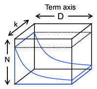
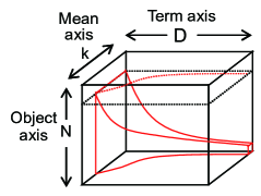
Figure 12: Conceptual diagram of number of multiplications executed in triple loop of (a) IFN and (b) IVF. Numbers correspond to volumes surrounded by curves illustrated in rectangles.

7 Discussion

We compare IVF with two similar algorithms, IFN in Section 4 and IVFD that is related to wand-k-means [29] in Section 2.3, and discuss their performances.

7.1 IFN and IVF

IFN operated in less CPU time than IVF in the small $k$ range in Figs. 5(a) and (b). From the viewpoints of the performance degradation factors, IVF was inferior in this range to IFN based on the number of instructions in Figs. 6(a) and (b). We focus on the number of instructions needed by each algorithm, especially in the triple loop at the assignment step because most of the CPU time was spent in the triple loop based on our preliminary analyses.

Table III shows an overview of the triple loops in IFN and IVF. The two algorithms only differ in the innermost loop labeled as 3. IFN loads feature value $u_{(s,j)}$ in the $j$-th entry in array $\bar{\bm{\xi}}_{s}$ from an external memory or a cache, multiplies $u_{(s,j)}$ with $v_{(i,h)}$, and adds a multiplication value to partial similarity $\rho_{j}$. This procedure is repeated by

$$k\cdot\sum_{i=1}^{N}(nt)_{i}=\sum_{i=1}^{N}\sum_{h=1}^{(nt)_{i}}k\>,$$ (12)

where the number of repetitions corresponds to the number of multiplications. By contrast, IVF loads the tuple of mean ID $c_{(s,q)}$ and feature value $u_{(s,q)}$ in the $q$-th entry in array $\breve{\bm{\xi}}_{s}$. The number of repetitions of the foregoing procedure is expressed by

$$\sum_{i=1}^{N}\sum_{h=1}^{(nt)_{i}}(nc)_{s},\>~{}~{}~{}\>s=t_{(i,h)}\>.$$ (13)

Figures 12(a) and (b) intuitively clarify the number of multiplications. This shows a conceptual diagram of the number of multiplications executed in the triple loops by IFN and IVF. The number of multiplications is represented as the volume surrounded by the curves in the rectangle. The curve in the (Term axis)-(Object axis) plane, which is shared by the two algorithms, depicts a distribution of objects each of whose feature vectors contains a value of the corresponding term. The area surrounded by the curve in Fig. 12(a) is $\sum_{i=1}^{N}(nt)_{i}$, and the volume is expressed by Eq. (12) for IFN. The curve in the (Term axis)-(Mean axis) plane in Fig. 12(b) illustrates the distribution of means, each of whose feature vectors contains a value of the corresponding term. The volume of IVF is expressed by Eq. (13). Figures 13(a) and (b) show the numbers of multiplications executed by IFN and IVF in their triple loops. The number of multiplications by IVF is smaller than that by IFN in every $k$ range, and such differences gradually increase with $k$, i.e., where the increase of IVF’s curve is suppressed. This is because the average sparsity of the mean feature vectors decreases with $k$ (Fig. 3(b)).

(a) PubMed	(b) NYT

\psfrag{K}[c][c][0.9]{ \begin{picture}(0.0,0.0)\put(0.0,0.0){\makebox(0.0,-6.0)[c]{Number of clusters: $k$} } \end{picture} }\psfrag{W}[c][c][0.9]{ \begin{picture}(0.0,0.0)\put(0.0,0.0){\makebox(0.0,30.0)[c]{\# multiplications} } \end{picture} }\psfrag{P}[l][r][0.82]{$10^{2}$}\psfrag{Q}[c][c][0.82]{$10^{3}$}\psfrag{R}[c][c][0.82]{$10^{4}$}\psfrag{X}[r][r][0.82]{$10^{10}$}\psfrag{Y}[r][r][0.82]{$10^{11}$}\psfrag{Z}[r][r][0.82]{$10^{12}$}\psfrag{A}[r][r][0.65]{{\em IVF}}\psfrag{B}[r][r][0.65]{{\em IFN}}\includegraphics[width=108.12047pt]{./vol_pubmed1M.eps}

\psfrag{K}[c][c][0.9]{Number of clusters: $k$}\psfrag{W}[c][c][0.9]{ \begin{picture}(0.0,0.0)\put(0.0,0.0){\makebox(0.0,30.0)[c]{\# multiplications}} \end{picture} }\psfrag{P}[l][r][0.82]{$10^{2}$}\psfrag{Q}[c][c][0.82]{$10^{3}$}\psfrag{R}[c][c][0.82]{$10^{4}$}\psfrag{X}[r][r][0.82]{$10^{10}$}\psfrag{Y}[r][r][0.82]{$10^{11}$}\psfrag{Z}[r][r][0.82]{$10^{12}$}\psfrag{S}[r][r][0.82]{$10^{13}$}\psfrag{A}[r][r][0.65]{{\em IVF}}\psfrag{B}[r][r][0.65]{{\em IFN}}\includegraphics[width=108.12047pt]{./vol_nyt1M.eps}

Figure 13: Number of multiplications in triple loop in log-log scale for (a) PubMed and (b) NYT

(a) PubMed	(b) NYT

\psfrag{K}[c][c][0.9]{ \begin{picture}(0.0,0.0)\put(0.0,0.0){\makebox(0.0,-6.0)[c]{Number of clusters: $k$} } \end{picture} }\psfrag{W}[c][c][0.9]{ \begin{picture}(0.0,0.0)\put(0.0,0.0){\makebox(0.0,30.0)[c]{\# instructions} } \end{picture} }\psfrag{P}[l][r][0.82]{$10^{2}$}\psfrag{Q}[c][c][0.82]{$10^{3}$}\psfrag{R}[c][c][0.82]{$10^{4}$}\psfrag{X}[r][r][0.82]{$10^{11}$}\psfrag{Y}[r][r][0.82]{$10^{12}$}\psfrag{Z}[r][r][0.82]{$10^{13}$}\psfrag{S}[r][r][0.82]{$10^{14}$}\psfrag{A}[r][r][0.65]{{\em IVF}}\psfrag{B}[r][r][0.65]{{\em IFN}}\includegraphics[width=113.81102pt]{./inst_loop_pubmed1M.eps}

\psfrag{K}[c][c][0.9]{Number of clusters: $k$}\psfrag{W}[c][c][0.9]{ \begin{picture}(0.0,0.0)\put(0.0,0.0){\makebox(0.0,30.0)[c]{\# instructions}} \end{picture} }\psfrag{P}[l][r][0.82]{$10^{2}$}\psfrag{Q}[c][c][0.82]{$10^{3}$}\psfrag{R}[c][c][0.82]{$10^{4}$}\psfrag{Y}[r][r][0.82]{$10^{12}$}\psfrag{Z}[r][r][0.82]{$10^{13}$}\psfrag{S}[r][r][0.82]{$10^{14}$}\psfrag{T}[r][r][0.82]{$10^{15}$}\psfrag{A}[r][r][0.65]{{\em IVF}}\psfrag{B}[r][r][0.65]{{\em IFN}}\includegraphics[width=113.81102pt]{./inst_loop_nyt1M.eps}

Figure 14: Number of instructions in the triple loop in log-log scale for (a) PubMed and (b) NYT.

Assume that when a procedure for an entry in an array ($\bar{\bm{\xi}}_{s}$ or $\breve{\bm{\xi}}_{s}$) in the innermost loop is performed once, the numbers of instructions executed by IFN and IVF are $\alpha$ and $\beta$. Note that $\beta$ is larger than $\alpha$ by the number of instructions by which IVF loads the mean IDs, $c_{(s,q)}$, $q\!\in\!\{1,2,\cdots,(nc)_{s}\}$. We ignore the instructions for loading $(nc)_{s}$ itself due to their smaller numbers. Then the numbers of instructions are expressed by

$$\left\{\begin{array}[]{lll}\alpha\cdot\sum_{i=1}^{N}\sum_{h=1}^{(nt)_{i}}k&\mbox{for}&\mbox{\em IFN}\\ \beta\cdot\sum_{i=1}^{N}\sum_{h=1}^{(nt)_{i}}(nc)_{s}&\mbox{for}&\mbox{\em IVF}\end{array}\right.\>.$$ (14)

Both $\alpha$ and $\beta$ depend on the computer architecture on which the algorithms operate. The number of multiplications depends on the sparsity of the object feature vectors, and in IVF it furthermore depends on the sparsity of the mean feature vectors.

We obtained $\alpha\!=\!28$ and $\beta\!=\!40$ in our preliminary analysis of the assembly codes generated from the source codes of the algorithms and applied them to Eq. (14). Figures 14(a) and (b) show the results, which are compared to the average numbers of instructions per iteration in Figs. 6(a) and (b). The cross points of the two curves of IFN and IVF appeared at almost the same $k$ values in Figs. 14 and 6. We believe that the difference in the speed performance of IFN and IVF is mainly caused by the difference of the number of instructions in the triple loop.

We provide the condition that IVF achieves better performance than IFN as follows:

$$\frac{\alpha}{\beta}>\frac{\sum_{i=1}^{N}\sum_{h=1}^{(nt)_{i}}(nc)_{s}}{k\cdot\sum_{i=1}^{N}(nt)_{i}}=\frac{1}{k}\cdot\frac{\sum_{p=1}^{D}\{(nc)_{p}\!\times\!(no)_{p}\}}{\sum_{p=1}^{D}(no)_{p}}\>,$$ (15)

where $(nc)_{p}$ and $(no)_{p}$ denote the numbers of centroids (means) and objects that contain a term with global term ID $p$, i.e., $(nc)_{p}$ and $(no)_{p}$ are the centroid and document frequencies of the $p$-th term. Thus IVF operates faster than IFN when value ($\alpha/\beta$) that is determined by a computer architecture is larger than a right-hand side value in Eq. (15) that is determined by given data objects and generated $k$ means.

7.2 IVFD and IVF

Assume that both the object and mean feature vectors are represented with a sparse expression. This presents a problem: which feature vectors should be inverted to achieve high performance?

7.2.1 Inverted-File for Data Object Feature Vectors

To address the foregoing problem, we designed a Lloyd-type algorithm IVFD that applies the inverted-file data structure to the data object feature vectors described in Section 2.3. This approach is the same as that of wand-k-means [29], although it employs a heuristic search instead of a linear-scan search for determining the objects’ assignments to clusters. To focus on only the basic data structure, IVFD adopts a linear-scan search to find the most similar centroid (mean) when each mean feature vector is given as a query. To reduce the computational cost for updating the mean feature vectors, IVFD utilizes not only the inverted-file data structure but also the standard data structure for the object feature vectors at the expense of consuming double memory capacitance.

Algorithm 4   IVFD at the $r$-th iteration

1:Input: $\breve{\cal X}$ (sparse & inverted-file),   $\hat{\cal X}$ (sparse),  $\hat{\cal M}^{[r-1]}$, ($k$)

2:Output: ${\cal C}^{[r]}\!=\!\{C_{1}^{[r]},C_{2}^{[r]},\cdots,C_{k}^{[r]}\}$,  $\hat{\cal M}^{[r]}$ (sparse)

3:$C_{j}^{[r]}\leftarrow\emptyset$ ,  $j=1,2,\cdots,k$ 

4:{ $/\!/$– Assignment step –$/\!/$ }

5:$\bm{\rho}\!=\!(\rho_{1},\rho_{2},\cdots,\rho_{i},\cdots,\rho_{N})\!\leftarrow\!\bm{0}$

6:$\bm{\rho}_{max}\!=\!(\rho_{max(1)},\cdots,\rho_{max(i)},\cdots,\rho_{max(N)})\!\leftarrow\!\bm{0}$

7:for all $\hat{\bm{\mu}}_{j}^{[r-1]}\!=\![(\tau_{(j,h)},v^{\prime}_{(j,h)})_{h=1}^{(n\tau)_{j}}]^{[r-1]}\in\hat{\cal M}^{[r-1]}$   do

8:   $S^{\prime}_{j}\!=\!\{\tau_{(j,1)},~{}\tau_{(j,2)},~{}\cdots,~{}\tau_{(j,h)},~{}\cdots,~{}\tau_{(j,(n\tau)_{j})}\}$

9:   for all  $s\!\leftarrow\!\tau_{(j,h)}\in S^{\prime}_{j}$  do

10:      for all  $(o_{(s,q)},u_{(s,q)})\in\breve{\bm{\zeta}}_{s}$  do

11:          $\breve{\bm{\zeta}}_{s}\!=\!(o_{(s,q)},u_{(s,q)})_{q=1}^{(no)_{s}}\in\!\breve{\cal X}$

12:          $\rho_{o_{(s,q)}}\leftarrow\rho_{o_{(s,q)}}+v^{\prime}_{(j,h)}\!\times\!u_{(s,q)}$

13:      end for

14:   end for

15:   for   $i\!=\!1$ to  $N$  do

16:      if   $\rho_{i}\!>\!\rho_{max(i)}$  then  $\rho_{max(i)}\!\leftarrow\!\rho_{i}$ and $a(\hat{\bm{x}}_{i})\!\leftarrow\!j$

17:   end for

18:end for

19:for   $i\!=\!1$ to  $N$  do

20:   $C_{a(\hat{\bm{x}}_{i}})^{[r]}\leftarrow C_{a(\hat{\bm{x}}_{i})}^{[r]}\cup\{\hat{\bm{x}}_{i}\}$

21:end for

22:{ $/\!/$– Update step –$/\!/$ }

23:$h_{p}\!\leftarrow\!0$,   $p=1,2,\cdots,D$

24:for all $C_{j}^{[r]}\in{\cal C}^{[r]}$ do

25:   $\bm{w}\!=\!(w_{1},w_{2},\cdots,w_{D})\!\leftarrow\!\bm{0}$

26:   for all $\hat{\bm{x}}_{i}\!=\!(t_{(i,h)},v_{(i,h)})_{h=1}^{(nt)_{i}}\in C_{j}^{[r]}$ do

27:      for all $s\!\leftarrow\!t_{(i,h)}\in\{t_{(i,1)},\cdots,t_{(i,(nt)_{i})}\}$  do

28:         $w_{s}\!\leftarrow\!w_{s}\!+\!v_{(i,h)}$

29:      end for

30:   end for

31:   for  $p\!=\!1$  to  $D$  do  $w_{p}\!\leftarrow\!w_{p}/|C_{j}^{[r]}|$  end for

32:   for  $p\!=\!1$  to  $D$  do

33:      if  $w_{p}\!\neq\!0$   then

34:         $\tau_{(j,h_{p})}\!\leftarrow\!p$,   $v^{\prime}_{(j,h_{p})}\!\leftarrow\!w_{p}/\|\bm{w}\|_{2}$,   $h_{p}\!\leftarrow\!h_{p}\!+\!1$

35:      end if

36:   end for

37:end for

38:return  ${\cal C}^{[r]}\!=\!\{C_{1}^{[r]},C_{2}^{[r]},\cdots,C_{k}^{[r]}\}$,  $\hat{\cal M}^{[r]}$

Algorithm 4 shows the IVFD pseudocode at the $r$-th iteration. IVFD receives a set of the mean feature vectors represented by a standard data structure with sparse expression $\hat{\cal M}^{[r-1]}$ and uses two invariant object sets of the feature vectors with inverted-file sparse expression $\breve{\cal X}$ and standard sparse expression $\hat{\cal X}$ and returns cluster set ${\cal C}^{[r]}$ consisting of $k$ clusters and $\hat{\cal M}^{[r]}$. At the assignment step, similarities $\rho_{i}$, $i\!=\!1,\cdots,N$, between mean feature vector $\hat{\bm{\mu}}_{j}\!=\!(\tau_{(j,h)},v^{\prime}_{(j,h)})$ and every object feature vectors are calculated and stored, using inverted-file $\breve{\cal X}$ for the object features. Note that $\tau_{(j,h)}$ and $v^{\prime}_{(j,h)}$ denote the global term ID accessed by the tuple of mean ID $j$ and local counter $h$ and the corresponding feature value. The inverted-file $\breve{\cal X}$ consists of $D$ arrays $\breve{\bm{\zeta}}_{s}$ with $(no)_{s}$ entries, where $s\!=\!\tau_{(j,h)}$. The $q$-th entry in $\breve{\bm{\zeta}}_{s}$ is tuple $(o_{(s,q)},u_{(s,q)})$, where $q\!=\!1,2,\cdots,(no)_{s}$ and $o_{(s,q)}$ and $u_{(s,q)}$ denote the object ID $i$ ($o_{(s,q)}\!=\!i$) and the corresponding feature value. At the update step, mean feature vector with standard sparse expression $\hat{\bm{\mu}}_{j}^{[r]}$ is calculated using object feature vectors with standard sparse expression $\hat{\bm{x}}_{i}\!\in\!C_{j}^{[r]}$. This algorithm differs from that in Algorithm 3. However, the main difference between them is only the order of the triple loop and the data structures for the object feature vectors and the mean feature vectors.

7.2.2 Performance Comparison

IVFD and IVF were applied to PubMed for evaluating their performance. Figures 15(a) and (b) show the performance-comparison results in terms of the maximum memory capacitance required by the algorithms through iterations until the convergence and the average CPU time per iteration. The horizontal lines labeled 0.707 and 1.414 in Fig. 15(a) denote the memory capacitances occupied by the object feature vectors and the double capacitance. IVFD used double capacitance for the object feature vectors as designed. Regarding speed performance, IVFD needed more CPU time than IVF in all the $k$ ranges. The maximum and minimum rates of the IVFD’s CPU time to the IVF’s were 1.82 at $k\!=\!1,000$ and 1.55 at $k\!=\!20,000$. Although IVF employed the inverted-file data structure for the variable mean feature vectors at the update step, it operated faster than IVFD. This is because constructing the inverted-file mean feature vectors is not costly. Importantly, most CPU time is spent at not the update step but the assignment step. In particular, both the algorithms spent at least 92% of their CPU time for the triple loop in their assignment steps in all the $k$ ranges.

(a) Required memory size	(b) CPU time

\psfrag{K}[c][c][0.88]{ \begin{picture}(0.0,0.0)\put(0.0,0.0){\makebox(0.0,-6.0)[c]{Number of clusters: $k(\times 10^{3})$} } \end{picture} }\psfrag{W}[c][c][0.88]{ \begin{picture}(0.0,0.0)\put(0.0,0.0){\makebox(0.0,27.0)[c]{Max. memory size (GB)} } \end{picture} }\psfrag{O}[l][r][0.82]{0}\psfrag{P}[c][c][0.82]{5}\psfrag{Q}[c][c][0.82]{10}\psfrag{R}[c][c][0.82]{15}\psfrag{S}[c][c][0.82]{20}\psfrag{T}[r][r][0.82]{0}\psfrag{X}[r][r][0.82]{0.5}\psfrag{Y}[r][r][0.82]{1.0}\psfrag{Z}[r][r][0.82]{1.5}\psfrag{U}[r][r][0.82]{2.0}\psfrag{A}[r][r][0.65]{{\em IVF}}\psfrag{B}[r][r][0.65]{{\em IVFD}}\psfrag{C}[c][c][0.65]{0.707}\psfrag{D}[c][c][0.65]{1.414}\includegraphics[width=113.81102pt]{./ivfd_mem_pubmed1M.eps}

\psfrag{K}[c][c][0.9]{ \begin{picture}(0.0,0.0)\put(0.0,0.0){\makebox(0.0,-6.0)[c]{Number of clusters: $k$} } \end{picture} }\psfrag{W}[c][c][0.9]{ \begin{picture}(0.0,0.0)\put(0.0,0.0){\makebox(0.0,27.0)[c]{Avg. CPU time (sec)} } \end{picture} }\psfrag{P}[c][r][0.82]{$10^{2}$}\psfrag{Q}[c][c][0.82]{$10^{3}$}\psfrag{R}[c][c][0.82]{$10^{4}$}\psfrag{X}[r][r][0.82]{$10^{1}$}\psfrag{Y}[r][r][0.82]{$10^{2}$}\psfrag{Z}[r][r][0.82]{$10^{3}$}\psfrag{U}[r][r][0.82]{$10^{4}$}\psfrag{A}[r][r][0.65]{{\em IVF}}\psfrag{B}[r][r][0.65]{{\em IVFD}}\includegraphics[width=113.81102pt]{./ivfd_time_pubmed1M.eps}

Figure 15: Performance comparison of IVFD and IVF in PubMed: (a) Maximum memory size required through iterations is illustrated with $k$ and horizontal line of 0.707 indicates memory size occupied by object feature vectors. (b) Average CPU time per iteration is depicted with $k$ in log-log scale.

(a) Avg. #instructions	(b) Avg. #multiplications

\psfrag{K}[c][c][1.0]{Number of clusters: $k$}\psfrag{W}[c][c][0.9]{ \begin{picture}(0.0,0.0)\put(0.0,0.0){\makebox(0.0,31.0)[c]{Avg. \#instructions} } \end{picture} }\psfrag{P}[c][r][0.85]{$10^{2}$}\psfrag{Q}[c][c][0.85]{$10^{3}$}\psfrag{R}[c][c][0.85]{$10^{4}$}\psfrag{X}[r][r][0.85]{$10^{11}$}\psfrag{Y}[r][r][0.85]{$10^{12}$}\psfrag{Z}[r][r][0.85]{$10^{13}$}\psfrag{S}[r][r][0.85]{$10^{14}$}\psfrag{A}[r][r][0.68]{{\em IVF}}\psfrag{B}[r][r][0.68]{{\em IVFD}}\includegraphics[width=116.6563pt]{./ivfd_inst_pubmed1M.eps}

\psfrag{K}[c][c][1.0]{Number of clusters: $k$}\psfrag{W}[c][c][0.9]{ \begin{picture}(0.0,0.0)\put(0.0,0.0){\makebox(0.0,31.0)[c]{Avg. \#multiplications} } \end{picture} }\psfrag{P}[c][r][0.85]{$10^{2}$}\psfrag{Q}[c][c][0.85]{$10^{3}$}\psfrag{R}[c][c][0.85]{$10^{4}$}\psfrag{X}[r][r][0.85]{$10^{10}$}\psfrag{Y}[r][r][0.85]{$10^{11}$}\psfrag{Z}[r][r][0.85]{$10^{12}$}\psfrag{A}[r][r][0.68]{{\em IVF}}\psfrag{B}[r][r][0.68]{{\em IVFD}}\includegraphics[width=116.6563pt]{./ivfd_mult_pubmed1M.eps}

Figure 16: Comparison of IVFD and IVF in PubMed: (a) Average number of instructions per iteration. Values of two algorithms were almost equal. Absolute difference of values at each $k$ value was at most 0.7%. (b) Average number of multiplications in triple loop per iteration. Not only average but also exact numbers of multiplications for each iteration at each $k$ value were equal.

Figure 16(a) shows the average number of instructions executed in the triple loop at the assignment step per iteration, and Fig. 16(b) shows the average number of multiplications operated in the triple loop per iteration. The numbers of instructions executed by IVFD and IVF were almost equal. The absolute difference of the numbers of instructions of the algorithms at each $k$ value was at most 0.7%. Both used identical number of multiplications at each iteration. This can be confirmed by comparing Algorithm 4 with Algorithm 3. Both performed the multiplications illustrated as the volume in Fig. 12(b).

(a) CPI	(b) #L1-cache misses
(c) #LL-cache misses	(d) #branch mispredictions

\psfrag{K}[c][c][0.9]{ \begin{picture}(0.0,0.0)\put(0.0,0.0){\makebox(0.0,-6.0)[c]{Number of clusters: $k$} } \end{picture} }\psfrag{W}[c][c][1.0]{ \begin{picture}(0.0,0.0)\put(0.0,0.0){\makebox(0.0,24.0)[c]{CPI} } \end{picture} }\psfrag{P}[l][r][0.82]{$10^{2}$}\psfrag{Q}[c][c][0.82]{$10^{3}$}\psfrag{R}[c][c][0.82]{$10^{4}$}\psfrag{X}[r][r][0.82]{0}\psfrag{Y}[r][r][0.82]{0.1}\psfrag{Z}[r][r][0.82]{0.2}\psfrag{S}[r][r][0.82]{0.3}\psfrag{T}[r][r][0.82]{0.4}\psfrag{U}[r][r][0.82]{0.5}\psfrag{A}[r][r][0.65]{\em IVF}\psfrag{B}[r][r][0.65]{\em IVFD}\includegraphics[width=116.6563pt]{./ivfd_clk-inst_pubmed1M.eps}

\psfrag{K}[c][c][0.9]{ \begin{picture}(0.0,0.0)\put(0.0,0.0){\makebox(0.0,-6.0)[c]{Number of clusters: $k$} } \end{picture} }\psfrag{W}[c][c][0.9]{ \begin{picture}(0.0,0.0)\put(0.0,0.0){\makebox(0.0,22.0)[c]{L1CM${}^{\prime}$/~{}Inst $(\times\!10^{-3})$} } \end{picture} }\psfrag{P}[l][r][0.82]{$10^{2}$}\psfrag{Q}[c][c][0.82]{$10^{3}$}\psfrag{R}[c][c][0.82]{$10^{4}$}\psfrag{X}[r][r][0.82]{0}\psfrag{Y}[r][r][0.82]{5}\psfrag{Z}[r][r][0.82]{10}\psfrag{S}[r][r][0.82]{15}\psfrag{T}[r][r][0.82]{20}\psfrag{A}[r][r][0.65]{{\em IVF}}\psfrag{B}[r][r][0.65]{{\em IVFD}}\includegraphics[width=116.6563pt]{./ivfd_l1cm-inst_pubmed1M.eps}

\psfrag{K}[c][c][0.9]{ \begin{picture}(0.0,0.0)\put(0.0,0.0){\makebox(0.0,-6.0)[c]{Number of clusters: $k$} } \end{picture} }\psfrag{W}[c][c][0.9]{ \begin{picture}(0.0,0.0)\put(0.0,0.0){\makebox(0.0,18.0)[c]{LLCM~{}/~{}Inst $(\times\!10^{-3})$} } \end{picture} }\psfrag{P}[l][r][0.82]{$10^{2}$}\psfrag{Q}[c][c][0.82]{$10^{3}$}\psfrag{R}[c][c][0.82]{$10^{4}$}\psfrag{X}[r][r][0.82]{0}\psfrag{Y}[r][r][0.82]{1}\psfrag{Z}[r][r][0.82]{2}\psfrag{S}[r][r][0.82]{3}\psfrag{T}[r][r][0.82]{4}\psfrag{A}[r][r][0.65]{{\em IVF}}\psfrag{B}[r][r][0.65]{{\em IVFD}}\includegraphics[width=116.6563pt]{./ivfd_llcm-inst_pubmed1M.eps}

\psfrag{K}[c][c][0.9]{ \begin{picture}(0.0,0.0)\put(0.0,0.0){\makebox(0.0,-6.0)[c]{Number of clusters: $k$} } \end{picture} }\psfrag{W}[c][c][0.9]{ \begin{picture}(0.0,0.0)\put(0.0,0.0){\makebox(0.0,31.0)[c]{BM/~{}Inst} } \end{picture} }\psfrag{P}[l][r][0.82]{$10^{2}$}\psfrag{Q}[c][c][0.82]{$10^{3}$}\psfrag{R}[c][c][0.82]{$10^{4}$}\psfrag{X}[r][r][0.82]{$10^{-6}$}\psfrag{Y}[r][r][0.82]{$10^{-5}$}\psfrag{Z}[r][r][0.82]{$10^{-4}$}\psfrag{S}[r][r][0.82]{$10^{-3}$}\psfrag{A}[r][r][0.65]{{\em IVF}}\psfrag{B}[r][r][0.65]{{\em IVFD}}\includegraphics[width=116.6563pt]{./ivfd_bm-inst_pubmed1M.eps}

Figure 17: Comparison of performance degradation factor characteristics obtained by IVFD and IVF in PubMed: (a) Clock cycles per instruction (CPI), (b) Difference of numbers of L1-cache and LL-cache misses per instruction, (c) Number of LL-cache misses per instruction, and (d) Number of branch mispredictions per instruction in log-log scale.

7.2.3 Analysis Based on CPI Model

To identify why IVFD needed more CPU time despite executing almost the same number of instructions as IVF, we analyzed IVFD from the viewpoint of performance degradation factors (DFs) and compared it with IVF. Figures 17(a), (b), (c), and (d) show CPI, the number of L1-data cache misses excluding the LL-cache misses (LLCM^′) per instruction, the number of LL-cache misses (LLCM) per instruction, and the number of branch mispredictions (BM) per instruction, respectively.

The difference in the CPIs in Fig. 17(a) corresponds to the CPU time in Fig. 15(b) since the numbers of instructions executed by both algorithms were almost identical. Actually, the IVF’s CPI ranged from 0.27 to 0.31, and IVFD’s ranged from 0.47 to 0.48. The rates of the IVFD’s CPIs to the IVF’s at $k\!=\!1,000,~{}20,000$ were 1.82 and 1.54, nearly equal to the CPU time rates. In Fig. 17(d), IVF had more branch mispredictions than IVFD. However, the number was too small, compared with those of the other DFs; its contribution to the CPU time can be ignored, as shown in Fig. 19(b). The difference in the CPU times (the clock cycles) came from the number of cache misses in Figs. 17(b) and (c). IVFD’s L1CM^′ and LLCM per instruction were constant high values. By contrast, IVF’s L1CM^′ and LLCM per instruction increased with $k$. These characteristics of the LLCMs are explained based on our cache-miss models in Section 7.2.4.

TABLE IV: Optimized CPI model parameters and errors on actual CPIs

Algo.	Parameters				Avg. err.	Max. err.
	$w_{0}$	$w_{1}$	$w_{2}$	$w_{3}$	(%)	(%)
IVFD	0.243	8.94	16.8	23.8	0.445	1.52
IVF	0.243	3.13	13.5	23.8	0.461	3.19

\psfrag{K}[c][c][1.0]{ \begin{picture}(0.0,0.0)\put(0.0,0.0){\makebox(0.0,-6.0)[c]{Number of clusters: $k$} } \end{picture} }\psfrag{W}[c][c][1.1]{ \begin{picture}(0.0,0.0)\put(0.0,0.0){\makebox(0.0,20.0)[c]{CPI} } \end{picture} }\psfrag{P}[c][r][0.9]{$10^{2}$}\psfrag{Q}[c][c][0.9]{$10^{3}$}\psfrag{R}[c][c][0.9]{$10^{4}$}\psfrag{X}[r][r][0.9]{0}\psfrag{Y}[r][r][0.9]{0.1}\psfrag{Z}[r][r][0.9]{0.2}\psfrag{S}[r][r][0.9]{0.3}\psfrag{T}[r][r][0.9]{0.4}\psfrag{U}[r][r][0.9]{0.5}\psfrag{A}[r][r][0.75]{\em IVF}\psfrag{B}[r][r][0.75]{\em IVFD}\psfrag{M}[r][r][0.75]{Model}\includegraphics[width=156.49014pt]{./fit_ivfd_pubmed1M.eps}

Figure 18: Actual and model CPI of IVFD and IVF along $k$ in PubMed

We optimized the IVFD parameters by referring to the procedure in Section 6.2 to determine the contribution rates of the DFs to the CPU time. We assumed for the optimization that parameters $w_{0}$ and $w_{3}$ of IVFD in Eq. (9) were fixed at the same values as those of IVF. The optimized parameters and results are shown in Table IV and Fig. 18. The optimized CPI model agrees well with the actual CPIs since the average error and the maximum error in IVFD were 0.445% and 1.52%. Parameters $w_{1}$ and $w_{2}$ were larger than those of IVF; the stall clock cycles per cache miss were longer. Thus IVFD had more cache misses, each of which induced longer stall clock cycles.

(a) IVFD	(b) IVF

\psfrag{K}[c][c][0.9]{ \begin{picture}(0.0,0.0)\put(0.0,0.0){\makebox(0.0,-5.0)[c]{Number of clusters: $k(\times 10^{3})$} } \end{picture} }\psfrag{W}[c][c][0.9]{ \begin{picture}(0.0,0.0)\put(0.0,0.0){\makebox(0.0,22.0)[c]{Contribution rate} } \end{picture} }\psfrag{A}[c][c][0.86]{0.2}\psfrag{B}[c][c][0.86]{0.5}\psfrag{C}[c][c][0.86]{1}\psfrag{D}[c][c][0.86]{2}\psfrag{E}[c][c][0.86]{5}\psfrag{F}[c][c][0.86]{10}\psfrag{G}[c][c][0.86]{20}\psfrag{X}[r][r][0.86]{0}\psfrag{Y}[r][r][0.86]{0.2}\psfrag{Z}[r][r][0.86]{0.4}\psfrag{S}[r][r][0.86]{0.6}\psfrag{T}[r][r][0.86]{0.8}\psfrag{U}[r][r][0.86]{1.0}\psfrag{P}[r][r][0.86]{L1CM${}^{\prime}$}\psfrag{Q}[r][r][0.86]{LLCM}\includegraphics[width=116.6563pt]{./ivfd_contrib_pubmed1M.eps}

\psfrag{K}[c][c][0.9]{ \begin{picture}(0.0,0.0)\put(0.0,0.0){\makebox(0.0,-5.0)[c]{Number of clusters: $k(\times 10^{3})$} } \end{picture} }\psfrag{W}[c][c][0.9]{ \begin{picture}(0.0,0.0)\put(0.0,0.0){\makebox(0.0,22.0)[c]{Contribution rate} } \end{picture} }\psfrag{A}[c][c][0.86]{0.2}\psfrag{B}[c][c][0.86]{0.5}\psfrag{C}[c][c][0.86]{1}\psfrag{D}[c][c][0.86]{2}\psfrag{E}[c][c][0.86]{5}\psfrag{F}[c][c][0.86]{10}\psfrag{G}[c][c][0.86]{20}\psfrag{X}[r][r][0.86]{0}\psfrag{Y}[r][r][0.86]{0.2}\psfrag{Z}[r][r][0.86]{0.4}\psfrag{S}[r][r][0.86]{0.6}\psfrag{T}[r][r][0.86]{0.8}\psfrag{U}[r][r][0.86]{1.0}\psfrag{O}[r][r][0.86]{Inst}\psfrag{R}[r][r][0.86]{BM}\includegraphics[width=116.6563pt]{./ivf_contrib_pubmed1M.eps}

Figure 19: Contribution rate of each DF to CPU time when (a) IVFD and (b) IVF were applied to PubMed. DFs are Inst, L1CM^′, LLCM, and BM.

Figures 19(a) and (b) show the contribution rates of each DF to the CPU times in IVFD and IVF. The rates of L1CM^′ and LLCM were high in IVFD, and the rate of Inst occupied much of the whole of contribution rate in IVF. In terms of branch misprediction (BM), its contribution rates in IVFD and IVF were very small, and we can ignore its values. Since the number of instructions and parameter $w_{0}$ were equal in IVFD and IVF, the IVFD’s performance degradation was caused by cache misses, more of which were caused by the long arrays $\bm{\zeta}_{s}$ of object inverted-file $\breve{\cal X}$ in the innermost loop in the triple loop in Algorithm 4.

7.2.4 LL-Cache-Miss Models for IVFD and IVF

Figure 17(c) shows that the number of last-level cache misses (LLCM) of IVF increased with $k$ while that of IVFD was almost constant in the $k$ range. We analyzed these characteristics.

The last-level (LL) cache used in our experiments contained 36,700,160 (35 M) bytes in 64-byte blocks with 20-way set associative placement and least-recently used (LRU) replacement. Instead of the actual set associative replacement, we assumed fully associative one in our analysis. Both IVFD and IVF used an inverted-file data structure that consisted of two arrays for 4-byte IDs of objects or centroids and 8-byte feature values.

IVF calculates similarities (inner products) between an object and all centroids (means) in the middle and innermost loop in the triple loop at its assignment step. A probability that a term with global term ID $p$ is used for a similarity calculation is $(no)_{p}/N$, where $(no)_{p}$ denotes the number of objects that contain the $p$-th term, i.e., the document frequency of the term. When the array related to the $p$-th term, $\breve{\bm{\xi}}_{p}\!=\!(c_{(p,q)},u_{(p,q)})_{q=1}^{(nc)_{p}}\!\in\!\breve{\cal M}$, is accessed, the number of blocks (NB${}_{[\mbox{\tiny\em IVF}]}$) that are placed into the LL cache from the main memory is given by

$$\mbox{\em NB}_{[\mbox{\tiny\em IVF}]}=\left\lceil(nc)_{p}\times\frac{\mbox{sizeof(int + double)}}{\mbox{block size}}\right\rceil\>,$$ (16)

where $(nc)_{p}$ denotes the number of centroids that contain the $p$-th term and depends on $k$. Then the expected number of blocks that are placed into the LL cache is expressed by

$$\mathbb{E}[\mbox{\em NB}_{[\mbox{\tiny\em IVF}]}]=\sum_{p=1}^{D}\frac{(no)_{p}}{N}\cdot\left\lceil(nc)_{p}\cdot\gamma\right\rceil\>,$$ (17)

where $\gamma$ denotes (sizeof(int + double))/(block size). By contrast, when IVFD calculates similarities between a centroid and all objects, the expected number of blocks (NB${}_{[\mbox{\tiny\em IVFD}]}$) is expressed by

$$\mathbb{E}[\mbox{\em NB}_{[\mbox{\tiny\em IVFD}]}]=\sum_{p=1}^{D}\frac{(nc)_{p}}{k}\cdot\left\lceil(no)_{p}\cdot\gamma\right\rceil\>.$$ (18)

Assume that $(nc)_{p}\cdot\gamma$ and $(no)_{p}\cdot\gamma$ are integers. Then Eqs. (17) and (18) are simplified:

$$\mathbb{E}[\mbox{\em NB}_{[\mbox{\tiny\em IVF}]}] = \frac{1}{N}\left(\gamma\textstyle{\sum_{p=1}^{D}(no)_{p}(nc)_{p}}\right)$$ (19)

$$\mathbb{E}[\mbox{\em NB}_{[\mbox{\tiny\em IVFD}]}] = \frac{1}{k}\left(\gamma\textstyle{\sum_{p=1}^{D}(no)_{p}(nc)_{p}}\right)\>,$$ (20)

where $\sum_{p=1}^{D}(no)_{p}(nc)_{p}$ is the number of multiplications that is illustrated as the volume in Fig. 12(b). It is clear that

$$\mathbb{E}[\mbox{\em NB}_{[\mbox{\tiny\em IVF}]}]\ll\mathbb{E}[\mbox{\em NB}_{[\mbox{\tiny\em IVFD}]}]~{}~{}~{}~{}(N\gg k)\>.$$ (21)

We compare $\mathbb{E}[\mbox{\em NB}_{[\mbox{\tiny\em IVF}]}]$ and $\mathbb{E}[\mbox{\em NB}_{[\mbox{\tiny\em IVFD}]}]$ with the number of blocks in the actual LL cache when IVF and IVFD are applied to PubMed ($N\!=\!1\!\times\!10^{6}$), given $k\!=\!1\!\times\!10^{4}$. In this comparison, we assume that the number of available blocks ($\mbox{\em NB}_{[\mbox{\tiny\em LLC}]}$) is $5\!\times\!10^{5}$ that corresponds to 32 MB. The number of multiplications executed by IVF was $2.21\!\times\!10^{11}$ shown in Fig. 13(a) and $\gamma\!=\!(4+8)/64\!=\!3/16$. Then $\mathbb{E}[\mbox{\em NB}_{[\mbox{\tiny\em IVF}]}]\!\sim\!4\!\times\!10^{4}$ and $\mathbb{E}[\mbox{\em NB}_{[\mbox{\tiny\em IVFD}]}]\!\sim\!4\!\times\!10^{6}$. The inequality in Eq. (21) is rewritten as

$$\mathbb{E}[\mbox{\em NB}_{[\mbox{\tiny\em IVF}]}]\ll\mbox{\em NB}_{[\mbox{\tiny\em LLC}]}\ll\mathbb{E}[\mbox{\em NB}_{[\mbox{\tiny\em IVFD}]}]\>.$$ (22)

This inequality held in the $k$ range from 200 to 20,000 when the algorithms were applied to PubMed.

The fact of $\mathbb{E}[\mbox{\em NB}_{[\mbox{\tiny\em IVFD}]}]\!\gg\!\mbox{\em NB}_{[\mbox{\tiny\em LLC}]}$ means that IVFD almost always fails to use feature values in the LL cache like cold-start misses. Based on this, we assume that the blocks required by IVFD must be always brought into the LL cache from the main memory. Then the number of LL-cache misses (LLCM${}_{[\mbox{\tiny\em IVFD}]}$) is given by

$$\mbox{LLCM}_{[\mbox{\tiny\em IVFD}]} = \textstyle{\sum_{p=1}^{D}(nc)_{p}\lceil(no)_{p}\cdot\gamma\rceil}$$ (23)

$$\sim \gamma\textstyle{\sum_{p=1}^{D}(no)_{p}(nc)_{p}}\>.$$ (24)

We show the rate of LLCM${}_{[\mbox{\tiny\em IVFD}]}$ in Eq. (23) to the number of instructions (Inst${}_{[\mbox{\tiny\em IVFD}]}$) that was obtained in our experiments as Model in Fig. 20. The model curve coincided with the actual rate depicted as IVFD in Fig. 17(c). Furthermore, we approximate the rate as

$$\frac{\mbox{LLCM}_{[\mbox{\tiny\em IVFD}]}}{\mbox{Inst}_{[\mbox{\tiny\em IVFD}]}}\sim\frac{\gamma\sum_{p=1}^{D}(no)_{p}(nc)_{p}}{\beta\times\mbox{(\#multiplications)}}=\frac{\gamma}{\beta}\>,$$ (25)

where $\beta$ is the same constant value as that for IVF in Eq. (14) and #multiplications denotes $\sum_{p=1}^{D}(no)_{p}(nc)_{p}$. Since $\beta\!=\!40$ and $\gamma\!=\!3/16$ in our experiments, $\mbox{LLCM}_{[\mbox{\tiny\em IVFD}]}/\mbox{Inst}_{[\mbox{\tiny\em IVFD}]}\!=\!4.7\!\times\!10^{-3}$. This approximate value is not so far from the IVFD values in Fig. 17(c) and higher than the corresponding values in Fig. 20 because $\beta\!\times\!\mbox{(\#multiplications)}$ is slightly smaller than actual Inst${}_{[\mbox{\tiny\em IVFD}]}$. Thus $\mbox{LLCM}_{[\mbox{\tiny\em IVFD}]}/\mbox{Inst}_{[\mbox{\tiny\em IVFD}]}$ becomes the constant value depending on the computer architecture.

\psfrag{K}[c][c][1.0]{ \begin{picture}(0.0,0.0)\put(0.0,0.0){\makebox(0.0,-6.0)[c]{Number of clusters: $k$} } \end{picture} }\psfrag{W}[c][c][0.9]{ \begin{picture}(0.0,0.0)\put(0.0,0.0){\makebox(0.0,18.0)[c]{LLCM~{}/~{}Inst $(\times\!10^{-3})$} } \end{picture} }\psfrag{P}[l][r][0.9]{$10^{2}$}\psfrag{Q}[c][c][0.9]{$10^{3}$}\psfrag{R}[c][c][0.9]{$10^{4}$}\psfrag{X}[r][r][0.9]{0}\psfrag{Y}[r][r][0.9]{1}\psfrag{Z}[r][r][0.9]{2}\psfrag{S}[r][r][0.9]{3}\psfrag{T}[r][r][0.9]{4}\psfrag{A}[r][r][0.75]{{\em IVF}}\psfrag{B}[r][r][0.75]{{\em IVFD}}\psfrag{C}[r][r][0.75]{{Model}}\includegraphics[width=147.95433pt]{./comp_llcm-inst_pubmed1M.eps}

Figure 20: Actual and model (LLCM/Inst) of IVFD and IVF along $k$ in PubMed

Next, we model the IVF LLCM (LLCM${}_{[\mbox{\tiny\em IVF}]}$). When IVF calculates similarities among successive $z$ objects and all centroids, the expected number of blocks that are placed into the LL cache ($\mathbb{E}[\mbox{\em NB}_{[\mbox{\tiny\em IVF}]}^{(z)}]$) is given by

$$\mathbb{E}[\mbox{\em NB}_{[\mbox{\tiny\em IVF}]}^{(z)}]=\sum_{p=1}^{D}\left\{1-\left(1-\frac{(no)_{p}}{N}\right)^{z}\right\}\lceil(nc)_{p}\gamma\rceil\>.$$ (26)

Note that $\mathbb{E}[\mbox{\em NB}_{[\mbox{\tiny\em IVF}]}^{(1)}]\!=\!\mathbb{E}[\mbox{\em NB}_{[\mbox{\tiny\em IVF}]}]$ in Eq. (17). Let $z^{*}$ denote the maximum integer $z$ under the condition that $\mathbb{E}[\mbox{\em NB}_{[\mbox{\tiny\em IVF}]}^{(z)}]$ satisfies

$$\mathbb{E}[\mbox{\em NB}_{[\mbox{\tiny\em IVF}]}^{(z)}]\leq\mbox{\em NB}_{[\mbox{\tiny\em LLC}]}\>.$$ (27)

When $z\!=\!z^{*}$, intuitively, the LL cache is fully occupied by arrays $\breve{\bm{\xi}}_{t_{(i,h)}}\!\in\!\breve{\cal M}$ related to terms that successive $z^{*}$ objects $\hat{\bm{x}}_{i}$ contain. Consider that when the LL cache is at this state, IVF requires array $\breve{\bm{\xi}}_{p}$ related to the $p$-th term, which is not placed in the LL cache. Then the expected number of blocks that are placed into the LL cache ($\mathbb{E}[\mbox{\em NB}_{[\mbox{\tiny\em IVF}]}^{(z^{*},\mbox{\scriptsize miss})}]$) is given by

$$\mathbb{E}[\mbox{\em NB}_{[\mbox{\tiny\em IVF}]}^{(z^{*},\mbox{\scriptsize miss})}]=\sum_{p=1}^{D}\frac{(no)_{p}}{N}\left(1-\!\frac{(no)_{p}}{N}\right)^{z^{*}}\left\lceil(nc)_{p}\gamma\right\rceil\>.$$ (28)

Using this value, LLCM${}_{[\mbox{\tiny\em IVF}]}$ is given and approximated as

$$\mbox{LLCM}_{[\mbox{\tiny\em IVF}]} = N\cdot\mathbb{E}[\mbox{\em NB}_{[\mbox{\tiny\em IVF}]}^{(z^{*},\mbox{\scriptsize miss})}]$$ (29)

$$\sim \gamma\sum_{p=1}^{D}(no)_{p}(nc)_{p}\left(1-\!\frac{(no)_{p}}{N}\right)^{z^{*}}\>.$$ (30)

The rate of LLCM${}_{[\mbox{\tiny\em IVF}]}$ in Eq. (29) to Inst${}_{[\mbox{\tiny\em IVF}]}$ in Fig. 17(c) is shown as Model in Fig. 20. The model curve gave close agreement with the values obtained by the experiments and increased with $k$. Furthermore, this rate is approximated as

$$\frac{\mbox{LLCM}_{[\mbox{\tiny\em IVF}]}}{\mbox{Inst}_{[\mbox{\tiny\em IVF}]}}\sim\left(\frac{\gamma}{\beta}\right)\frac{\sum_{p=1}^{D}(no)_{p}(nc)_{p}\left(1-\!\frac{(no)_{p}}{N}\right)^{z^{*}}}{\sum_{p=1}^{D}(no)_{p}(nc)_{p}}\>.$$ (31)

When $k$ approaches asymptotically to $N$, $z^{*}\!\rightarrow\!0$ and $(nc)_{p}\!\rightarrow\!(no)_{p}$ in Eq. (31). Then

$$\lim_{k\rightarrow N}\frac{\mbox{LLCM}_{[\mbox{\tiny\em IVF}]}}{\mbox{Inst}_{[\mbox{\tiny\em IVF}]}}\sim\frac{\gamma}{\beta}\sim\frac{\mbox{LLCM}_{[\mbox{\tiny\em IVFD}]}}{\mbox{Inst}_{[\mbox{\tiny\em IVFD}]}}\>.$$ (32)

$\mbox{LLCM}_{[\mbox{\tiny\em IVF}]}/\mbox{Inst}_{[\mbox{\tiny\em IVF}]}$ increases with $k$ and approached to $(\gamma/\beta)$ that is the approximate rate of IVFD.

Due to the reasons mentioned above, applying an inverted-file data structure to the mean feature vectors leads to better performance. We should use IVF rather than IVFD to achieve high performance for large-scale sparse data sets.

8 Conclusion

We proposed an inverted-file $k$-means clustering algorithm (IVF) that operated at high speed and with low memory consumption in large-scale high-dimensional sparse document data sets when large $k$ values were given. IVF represents both the given object feature vectors and the mean feature vectors with sparse expression to conserve occupied memory capacitance and exploits the inverted-file data structure for the mean feature vectors to achieve high-speed performance. We analyzed IVF using a newly introduced clock-cycle per instruction (CPI) model to identify factors for high-speed operation in a modern computer system. Consequently, IVF suppressed the three performance degradation factors of the numbers of cache misses, branch mispredictions, and completed instructions.

As future work, we will evaluate IVF in such practical environments as with parallel and distributed modern computer systems.

References

- [1] M. I. Jordan and T. M. Mitchell, “Machine learning: Trends, perspectives, and prospects,” Science, vol. 349, no. 6245, pp. 255–260, 2015.
- [2] X. Wu, V. Kumar, J. R. Quinlan, J. Ghosh, Q. Yang, H. Motoda, G. J. McLachlan, A. Ng, B. Liu, P. S. Yu, Z.-H. Zhou, M. Steinbach, D. J. Hand, and D. Steinberg, “Top 10 algorithms in data mining,” Knowl. Inf. Syst., vol. 14, no. 1, pp. 1–37, 2008.
- [3] S. P. Lloyd, “Least squares quantization in PCM,” IEEE Trans. Information Theory, vol. 28, no. 2, pp. 129–137, 1982.
- [4] J. B. MacQueen, “Some methods for classification and analysis of multivariate observations,” in Proc. 5th Berkeley Symp. Mathematical Statistics and Probability, 1967, pp. 281–297.
- [5] C. Elkan, “Using the triangle inequality to accelerate k-means,” in Proc. 20th Int. Conf. Machine Learning (ICML), 2003, pp. 147–153.
- [6] G. Hamerly, “Making k-means even faster,” in Proc. SIAM Int. Conf. Data Mining (SDM), 2010, pp. 130–140.
- [7] I. S. Dhillon and D. S. Modha, “Concept decompositions for large sparse text data using clustering,” Machine Learning, vol. 42, no. 1–2, pp. 143–175, 2001.
- [8] J. L. Hennessy and D. A. Patterson, Eds., Computer architecture, sixth edition: A quantitative approach. San Mateo, CA: Morgan Kaufmann, 2017.
- [9] M. Evers and T.-Y. Yeh, “Understanding branches and designing branch predictors for high-performance microprocessors,” Proc. IEEE, vol. 89, no. 11, pp. 1610–1620, 2001.
- [10] S. Eyerman, J. E. Smith, and L. Eeckhout, “Characterizing the branch misprediction penalty,” in Proc. Int. Symp. Perform. Anal. Syst. Softw. (ISPASS), 2006, pp. 48–58.
- [11] H. Samet, Ed., Foundations of multidimensional and metric data structures. San Francisco, CA, USA: Morgan Kaufmann Publishers Inc., 2006.
- [12] D. Harman, E. Fox, R. Baeza-Yates, and W. Lee, “Inverted files,” in Information retrieval: Data structures & algorithms, W. B. Frakes and R. Baeza-Yates, Eds. New Jersey: Prentice Hall, 1992, ch. 3, pp. 28–43.
- [13] D. E. Knuth, “Retrieval on secondary keys,” in The art of computer programming: Volume 3: Sorting and searching. Addison-Wesley Professinal, 1998, ch. 5.2.4 and 6.5.
- [14] J. Zobel and A. Moffat, “Inverted files for text search,” ACM Computing Surveys, vol. 38, no. 2, article 6, 2006.
- [15] S. Büttcher, C. L. A. Clarke, and G. V. Cormack, Eds., Information retrieval: Implementing and evaluating search engines. Cambridge, Massachusetts: The MIT Press, 2010.
- [16] Perf, “Linux profiling with performance counters,” 2019. [Online]. Available: https://perf.wiki.kernel.org/index.php
- [17] D. Aloise, A. Deshpande, P. Hansen, and P. Popat, “NP-hardness of Euclidean sum-of-squares clustering,” Machine Learning, vol. 75, pp. 245–248, 2009.
- [18] J. Drake and G. Hamerly, “Accelerated k-means with adaptive distance bounds,” in Proc. 5th NIPS Workshop on Optimization for Machine Learning, 2012.
- [19] Y. Ding, Y. Zhao, X. Shen, M. Musuvathi, and T. Mytkowicz, “Yinyang k-means: A drop-in replacement of the classic k-means with consistent speedup,” in Proc. 32nd Int. Conf. Machine Learning (ICML), 2015, pp. 579–587.
- [20] J. Newling and F. Fleuret, “Fast k-means with accurate bounds,” in Proc. 33rd Int. Conf. Machine Learning (ICML), 2016.
- [21] T. Hattori, K. Aoyama, K. Saito, T. Ikeda, and E. Kobayashi, “Pivot-based k-means algorithm for numerous-class data sets,” in Proc. SIAM Int. Conf. Mata Mining (SDM), 2016, pp. 333–341.
- [22] K. Aoyama, K. Saito, and T. Ikeda, “Accelerating a Lloyd-type k-means clustering algorithm with summable lower bounds in a lower-dimensional space,” IEICE Trans. Inf. & Syst., vol. E101-D, no. 11, pp. 2773–2782, 2018.
- [23] J. Sivic and A. Zisserman, “Video Google: A text retrieval approach to object matching in videos,” in Proc. IEEE Int. Conf. Computer Vision (ICCV), 2003, pp. 1470–1478.
- [24] H. Jégou, M. Douze, and C. Schmid, “Product quantization for nearest neighbor search,” IEEE Trans. Pattern Anal. Mach. Intell., vol. 33, no. 1, pp. 117–128, 2011.
- [25] A. Babenko and V. Lempitsky, “The inverted multi-index,” IEEE Trans. Pattern Anal. Mach. Intell., vol. 37, no. 6, pp. 1247–1260, 2015.
- [26] P. Indyk and R. Motwani, “Approximate nearest neighbors: Towards removing the curse of dimensionality,” in Proc. ACM Symp. Theory of Computing (STOC), 1998, pp. 604–613.
- [27] A. Andoni, M. Datar, N. Immorlica, P. Indyk, and V. Mirrojni, “Locality-sensitive hashing using stable distributions,” in Nearest-neighbor methods in learning and vision; Theory and practice, G. Shakhnarovich, T. Darrell, and P. Indyk, Eds. The MIT Press, 2005, ch. 3, pp. 61–72.
- [28] M. S. Charikar, “Similarity estimation techniques from rounding algorithms,” in Proc. ACM Symp. Theory of Computing (STOC), 2002, pp. 380–388.
- [29] A. Broder, L. Garcia-Pueyo, V. Josifovski, S. Vassilvitskii, and S. Venkatesan, “Scalable k-means by ranked retrieval,” in Proc. ACM Int. Conf. Web Search and Data Mining (WSDM), 2014, pp. 233–242.
- [30] L. Jian, C. Wang, Y. Liu, S. Liang, W. Yi, and Y. Shi, “Parallel data mining techniques on graphics processing unit with compute unified device architecture (CUDA),” J. Supercomput., vol. 64, pp. 942–967, 2013.
- [31] J. Bhimani, M. Leeser, and N. Mi, “Accelerating K-means clustering with parallel implementations and GPU computing,” in Proc. IEEE High Performance Extreme Computing Conf. (HPEC), 2015, pp. 233–242.
- [32] K. Kaligosi and P. Sanders, “How branch mispredictions affect quicksort,” in Algorithms-ESA2006. Lecture Notes in Computer Science, Y. Azar and T. Erlebach, Eds. Springer, Berlin, Heidelberg, 2006, pp. 780–791.
- [33] S. Edelkamp and A. Weiß, “BlockQuicksort: Avoiding branch mispredictions in quicksort,” ACM J. Exp. Algorithmics (JEA), vol. 24, no. 1, pp. 1.4:1–1.4:22, 2019.
- [34] O. Green, M. Dukhan, and R. Vuduc, “Branch-avoiding graph algorithms,” in Proc. ACM Symp. Parallelism in Algorithms and Architectures (SPAA), 2015, pp. 212–223.
- [35] M. Kowarschik and C. Weiß, “An overview of cache optimization techniques and cache-aware numerical algorithms,” in Algorithms for memory heirarchies, Lecture Notes in Computer Science, U. Meyer, P. Sanders, and J. Sibeyn, Eds. Berlin, Heidelberg: Springer, 2003, ch. 10, pp. 213–232.
- [36] M. Frigo, C. Leiserson, H. Prokop, and S. Ramachandran, “Cache-oblivious algorithms,” ACM Trans. Algorithms, vol. 8, no. 1, article 4, 2012.
- [37] A. Ghoting, G. Buehrer, S. Parthasarathy, D. Kim, A. Nguyen, Y.-K. Chen, and P. Dubey, “Cache-conscious frequent pattern mining on modern and emerging processors,” The VLDB Journal, vol. 16, no. 1, pp. 77–96, 2007.
- [38] M. Perdacher, C. Plant, and C. Böhm, “Cache-oblivious high-performance similarity join,” in Proc. Int. Conf. Management of Data (SIGMOD), 2019, pp. 87–104.
- [39] D. Dua and E. K. Taniskidou, “Bag of words data set (PubMed abstracts) in UCI machine learning repository,” 2017. [Online]. Available: http://archive.ics.uci.edu/ml
- [40] P. Hammarlund, A. J. Martinez, A. A. Bajwa, D. L. Hill, E. Hallnor, H. Jiang, M. Dixon, M. Derr, M. Hunsaker, R. Kumar, R. B. Osborne, R. Rajwar, R. Singhal, R. D’Sa, R. Chappell, S. Kaushik, S. Chennupaty, S. Jourdan, S. Gunther, T. Piazza, and T. Burton, “Haswell: The fourth-generation Intel core processor,” IEEE Micro, vol. 34, issue 2, pp. 6–20, 2014.
- [41] Intel Corp., “Disclosure of hardware prefetcher control on some Intel processors,” 2014. [Online]. Available: https://software.intel.com/en-us/ articles/disclosure-of-hw-prefetcher-control-on-some-intel-processors