Facilitating SQL Query Composition and Analysis

Abstract.

Formulating efficient SQL queries requires several cycles of tuning and execution, particularly for inexperienced users. We examine methods that can accelerate and improve this interaction by providing insights about SQL queries prior to execution. We achieve this by predicting properties such as the query answer size, its run-time, and error class. Unlike existing approaches, our approach does not rely on any statistics from the database instance or query execution plans. This is particularly important in settings with limited access to the database instance.

Our approach is based on using data-driven machine learning techniques that rely on large query workloads to model SQL queries and their properties. We evaluate the utility of neural network models and traditional machine learning models. We use two real-world query workloads: the Sloan Digital Sky Survey (SDSS) and the SQLShare query workload. Empirical results show that the neural network models are more accurate in predicting the query error class, achieving a higher F-measure on classes with fewer samples as well as performing better on other problems such as run-time and answer size prediction. These results are encouraging and confirm that SQL query workloads and data-driven machine learning methods can be leveraged to facilitate query composition and analysis.

1. Introduction

Formulating effective SQL queries is one of the main challenges of interacting with large relational databases. Particularly for inexperienced users, writing good SQL queries may require several cycles of tuning and execution. This diminishes the user experience, prevents them from easily accessing information (Jagadish et al., 2007), and can also be costly. For example, cloud-based services, such as Google BigQuery, charge their users for running queries (Inc., 2012b; Google, 2010; Inc., 2012a). Moreover, inefficient SQL queries can pose a burden on the database’s resources. Our focus in this work is on facilitating user interaction with the database by providing additional information about SQL queries prior to their execution.

We focus on two groups of users: end users and database administrators (DBAs). To help end users compose SQL queries, we study three problems: query answer size prediction, query run-time prediction, and query error prediction. We can save end users time and effort by pointing out when their queries are inefficient, unlikely to work at all, or are likely to take radically different time than they are expecting (and thus are likely to be not the queries that they are trying to write).

We also improve user interaction for DBAs. To characterize how end users and programs use the service, DBAs need to analyze incoming requests and queries and categorize them into classes of clients (Singh et al., 2007). This in turn allows them to improve service quality for end users. To help DBAs with this analysis, we study the problem of session type classification, which is the automatic identification of the class of clients that generated the queries in a session.

While we use estimates of SQL query properties to improve usability, these estimates have typically been used to improve tasks like admission control, access control, scheduling, and costing during query optimization (Li et al., 2012; Liu et al., 2015; Ganapathi et al., 2009; Akdere et al., 2012). Most of these studies, however, are based on manually constructed cost models in the query optimizer and require access to the database instance. But the analytical cost models in the query optimizer can be imprecise due to simplifying assumptions, e.g., uniform data distributions (Leis et al., 2015; Ganapathi et al., 2009; Ding et al., 2019). Moreover, access to the database instance can be infeasible in an increasingly large number of settings, e.g., cloud-based data warehouses like Google BigQuery (Google, 2010), databases on the hidden web, sources located behind wrappers in data integration systems (Bergamaschi et al., 2011), and instances with limited access due to cost or privacy issues (Google, 2010; Inc., 2012b, a; Hacigümüş et al., 2002). Due to these restrictions, there is growing need for work that does not assume direct access to database instances.

Our approach for modeling the queries and their properties relies on using  SQL query workloads, which contain logs of past queries submitted to the database. Query workloads are an alternative resource in settings with limited database instance access. They have been used to improve query performance estimates for tasks like query optimization and scheduling (Akdere et al., 2012; Li et al., 2012; Ganapathi et al., 2009; Liu et al., 2015). In addition to requiring access to the database instance and schema, these works examine synthetic or small-scale query workloads, e.g., TPC-H (TPC, 2018). They extract hand-engineered features from query execution plans, and apply a prediction model. However, synthetic and small-scale query workloads do not represent the full capacity and challenges of potential queries, as shown empirically in (Leis et al., 2015).

We use SQL query workloads that are large-scale and real-world and present an abundance of realistic usage patterns from a variety of different users. These workloads are broadly used and publicly available in scientific and academic research domains. Examples are the Sloan Digital Sky Survey (SDSS) query workload (Szalay et al., 2002; Raddick et al., 2014a, b) and SQLShare (Jain et al., 2016). Companies and organizations, such as Snowflake (Jain and Howe, 2018; Jain et al., 2018), often maintain their own large-scale private workloads. DBMSs support logging features that make it easy to generate and maintain these workloads.

When large-scale workloads do not exist for a database, knowledge learned from workloads over other databases may be used for query property prediction. Consequently, we define different query facilitation problem settings that vary in their data heterogeneity. This makes the prediction problem more challenging due to different underlying data distributions for the SQL query and the workload. These settings require models that generalize well and can transfer knowledge learned from workloads to predict query properties over a different database. We empirically show that some models generalize better, which allows reusing large-scale workloads for query performance property prediction. We hope in light of research like ours that shows the benefits of large-scale workloads, more companies and organizations develop, maintain, and share their query workloads, which can ultimately improve transparency and customer engagement.

We use data-driven machine learning techniques that require large-scale workloads to build effective models and predict different query properties. Since there are no standard models for our problems, we start by establishing appropriate baseline models. Our query facilitating problems are essentially query labeling tasks. A closely related area is text categorization, where the goal is to predict categories for documents written in natural language (Kim, 2014; Zhang et al., 2015; Conneau et al., 2016; Johnson and Zhang, 2014, 2015, 2016b, 2017). We chose a broad set of applicable models from this domain; on large-scale datasets, the dominant approaches use Long-Term Short-Term (LSTM) and Convolutional Neural Network (CNN) models (LeCun et al., 1989; Conneau et al., 2016; Bai et al., 2018; Yin et al., 2017). LSTMs treat texts as sequential inputs, while CNNs can automatically identify n-grams. SQL queries have significant differences with natural language sentences, e.g., they include mathematical expressions that are important to retain in the query representation. We therefore applied all models at both character and word level.

Our work is closest to (Jain and Howe, 2018; Jain et al., 2018), which assume no direct access to database instances and apply data-driven models to large-scale query workloads. They address workload management tasks, such as index recommendation and security audits. We introduce additional problems related to facilitating query composition and analysis, e.g., session classification. Moreover, we formalise and study different problem settings and conduct an extensive workload analysis that results in encouraging empirical results.

In summary we contribute the following:

• We motivate (Section 2) and formally define (Section 3) four problems that help end users and DBAs with composition and analysis by providing query insights prior to execution.

• Our approach relies on exploiting large query workloads. We use two real-world query workloads that are publicly available, SDSS and SQLShare. In Section 4, we describe these workloads. Moreover, to enable better model selection and evaluation, we conduct a comprehensive workload analysis that covers structural and syntactic features of the queries and their labels.

• We examine a broad set of models to establish the baselines and assess the feasibility of our problems in Section 5. We adapted two classes of neural network models to our problems and compared them with simple baselines and traditional NLP models.

• Our empirical evaluation (Section 6) shows the neural networks are more accurate in predicting the query error class, achieving a higher F-measure on classes with fewer samples. For run-time and answer size prediction, the neural networks obtain better results, particularly on complex queries. Additionally, we found character level CNNs are able to generalize better under various problem settings.

Section 7 describes related work and Section 8 concludes.

2. Motivating Example

⬇ SELECT COUNT(*) FROM Galaxy WHERE ...

(a) Users are advised to submit a count query before executing the actual query.

⬇ SELECT ... FROM PhotoObj WHERE flags & dbo.fPhotoFlags('BLENDED') > 0

(b) An inefficient query. It retrieves a large number of objects, the function call in the WHERE clause is called once per matching row.

Figure 1. Users are advised to optimize their queries on SDSS to prevent long wait times.

We use the Sloan Digital Sky Survey (SDSS) as a motivating example. SDSS is an astronomy project that provides a digital map of the sky (Raddick et al., 2014a, b; Szalay et al., 2002; Szalay, 2018). SDSS data includes raw images of the sky along with numerical estimates for the physical attributes of objects in the images. These numerical estimates, known as scientific attributes, are stored in the Catalog Archive Server (CAS) databases, which can be queried via SQL. Users access SDSS data through several access interfaces, including an asynchronous job interface called CasJobs and a web interface.  

A diverse set of end users, ranging from high school students to astronomers, with varied levels of astronomy and SQL knowledge, use SDSS (Szalay, 2018). To help users compose queries, SDSS provides some resources. These include a tutorial to help users learn SQL basics and a set of sample SQL queries that can be used as templates.   There are also descriptions of costly queries with hints on how to rewrite them to ensure they run faster.  For example, users are advised to always start with a “count” query (Figure 1a) to estimate of the query answer size and prevent long wait times. Figure 1 shows an inefficient query example, given on the SDSS website, which runs the function dbo.fPhotoFlags(’BLENDED’) for several records in PhotoObj. The users are advised to rewrite it to a query that invokes the function only once.  

While these resources are helpful, they are not sufficient. In particular, the step-by-step SQL tutorial is generic and helps inexperienced users learn SQL syntax rather than write meaningful queries. The sample set of queries is small and static compared to the size of the database and the complexity of potential queries. The SDSS schema has 87 tables, 46 views, 467 functions, 21 procedures, and 82 indices.  The schema size and complexity makes it hard for users to become familiar enough with the SDSS database to effectively optimize and tune their queries. Ad-hoc hints do not cover all possible optimization opportunities. In this context, real-time query performance estimates like answer size or execution time can increase user productivity and efficiency.

DBAs are another group who interact with SDSS. One of their tasks is to analyze the incoming requests and queries during a session and decide the class of the end user (e.g. human, bot, program) that generated the queries. This is called the session classification problem, where a session is defined as a sequence of interactions between an end user and the system. Session classification allows DBAs to improve the services offered based on usage patterns (Szalay et al., 2002).

Session classification is challenging. First, identifying individual sessions is difficult. This is because users are anonymous and do not necessarily login to the system, their IP addresses can change, and the same IP address can access different SDSS interfaces. In fact, there has been research on automatic session identification as a separate task (Khoussainova et al., 2010). We follow (Szalay et al., 2002) and assume that a session is characterized by an ordered sequence of hits (i.e., SQL query or web request) from a single IP address, such that the gaps between hits in the sequence is no longer than 30 minutes (Szalay et al., 2002; Raddick et al., 2014a).

The second step in session classification is specifying the correct label for an identified session. These labels can be used to enforce certain policies and optimize system services (e.g., for resource allocation, or to design different interaction modalities based on the usage patterns of different types of sessions (Szalay et al., 2002)). Although the web requests contain a string that describes the browser or program that generated the request, this “agent string” is not reliable. Consequently, SDSS user sessions are labeled using a combination of agent string, IP address, and behavior during session. This procedure does not consider the content or syntactic properties of queries. Therefore, a question that arises is whether the raw query itself can be used for performing the label assignment. This functionality would provide a complementary resource for assisting DBAs. Additionally, it helps automate identification of human traffic, which is needed for downstream usability problems, like query recommendation for end users (Khoussainova et al., 2010).

3. Problem Definition

We use small letters for scalars, capital letters for sets or sequences, bold small letters for vectors, and bold capital letters for matrices.

Definition 1.

A query $Q=(t_{1},...,t_{n})$ is a sequence of tokens from a vocabulary $V$. We consider two sets of vocabularies: a vocabulary that contains characters and a vocabulary that contains words. We define $v$ to denote the size of $V$ and $\mathcal{Q}$ denotes the collection of all queries over $V$. $\Box$

Example 3.1.

For the query in Figure 2a, $Q_{1}=$(“SELECT”, “*”, “FROM”, …) is a query with a vocabulary of words, and $Q_{2}=$ (‘S’, ‘E’, ‘L’, ‘E’, …) is a query with a vocabulary of characters.

Definition 2.

For a token $t_{i}$ in a query $Q$, we define $\bm{e}_{i}\in\{0,1\}^{v}$ as the one-hot encoding of $t_{i}$, i.e. a vector of bits for tokens in $V$ where the bit that corresponds to $t_{i}$ is $1$ and all the other bits are $0$. We use $\bm{x}_{i}\in\mathbb{R}^{d}$ to refer to the distributed representation of $t_{i}$ in latent space obtained using an embedding matrix $\bm{X}\in\mathbb{R}^{d\times v}$ ($\bm{x}_{i}=\bm{X}\bm{e}_{i}$). We define an $n$-gram in $Q$ as a sequence of $n$ tokens that appear in $Q$. $\Box$

Example 3.2.

The one-hot encoding of $t_{1}=$“SELECT” and $t_{2}=$“*” w.r.t. a vocabulary $V=\{t_{1},t_{2},t_{3},t_{4}\}$ is $\bm{e}_{1}=[1\;0\;0\;0]$ and $\bm{e}_{2}=[0\;1\;0\;0]$. Given an embedding matrix $\bm{X}=[[3\;6\;4]\;[9\;5\;8]\;[4\;3\;$ $0]\;[6\;0\;4]]$, $\bm{x}_{1}=[3\;6\;4]$ and $\bm{x}_{2}=[9\;5\;8]$ are the distributed representation of $t_{1}$ and $t_{2}$, respectively. The sequence (“SELECT”, “*”, “FROM”) is a $3$-gram of words and (‘F’,‘R’,‘O’,‘M’) is a $4$-gram of characters.

⬇ SELECT * FROM PhotoTag WHERE objId=0x112d075f80360018

(a) Error class: success, session class: bot, answer size: 1, and CPU time: 0.015

⬇ SELECT p.objid,p.ra,p.dec,p.u,p.g,p.r,p.i,p.z FROM PhotoObj AS p WHERE type=6 AND p.ra BETWEEN (156.519031-0.200000) AND (156.519031+0.200000) AND p.dec BETWEEN (62.835405-0.200000) AND (62.835405+0.200000) ORDER BY p.objid

(b) Error class: success, session class: browser, answer size: 98877, and CPU time: 41.342999

Figure 2. Example SQL queries in SDSS workload.

We want to model queries and their properties to generate feedback for end users and DBAs. Similar to (Bergamaschi et al., 2011), we assume a-priori access to the database instance, i.e., the tuples and their statistics, is not available. This is commonly the case for users of systems like SDSS, SQLShare, or web services like Google BigQuery. Instead, our approach exploits the rich content of large query workloads:

Definition 3.

[Query workload] Let $\mathcal{W}=\{(Q_{i},y_{i})\}_{i=1}^{n}$ denote the input query workload, where $Q_{i}$ is a query statement and $y_{i}$ is a query label. The label is a query property that is obtained by submitting $Q_{i}$ to the database. $\Box$

The query statement $Q_{i}$ is typically a SQL query and can contain clauses such as SELECT, EXECUTE, CREATE, ALTER, or combinations such as DELETE $|$ UPDATE $|$ INSERT clauses. However, in realistic workloads such as SDSS, the end user can submit any query to the system, including a random natural language sentence. So, the query type is not restricted.

The query label $y_{i}$ can correspond to different query properties, e.g., answer size or CPU time. We focus on four types of query labels. Our goal is to develop models that can predict these labels — prior to execution. For each query $Q_{i}$ the error class $y^{e}_{i}$ is a numeric indicator of whether the query successfully executed or not. The query total CPU time $y^{c}_{i}$ is a real number and represents the query execution time. The query answer size $y^{a}_{i}$ is an integer and represents the number of rows retrieved for the query. The session class $y^{s}_{i}$ is the class of client that generated the query (and its session). Figure 2 shows sample queries from our SDSS query workload, along with their properties.

Definition 4.

[Query Facilitation Problems] Given a query workload $\mathcal{W}=\{(Q_{i},$ $y_{i})\}_{i=1}^{n}$ and a query $Q_{*}$, a query facilitating problem is to predict the label $y_{*}$ of $Q_{*}$. We define four query facilitating problems depending on the label: error classification problem, CPU time prediction problem, answer size prediction problem, and session classification problem, where the label corresponds to either the error classes, CPU times, answer sizes, or the session classes. $\Box$

The underlying assumption in Definition 4 is that $Q_{*}$ and $\mathcal{W}$ have similar execution conditions, e.g., run over the same database instance. However, this restriction does not hold in many real applications. For example, cloud-based, multi-tenant, and multi-database platforms receive millions of queries from end users based on hundreds of schemas (Jain et al., 2018). It is vital to consider such settings and develop models that generalize well to unseen queries. Therefore, we relax this assumption and define the following settings.

Definition 5.

[Query Facilitation Problem Settings] Given a query workload $\mathcal{W}$ and a new query $Q_{*}$, the problems in Definition 4 can be studied under the following settings:

1. Homogeneous Instance: $Q_{*}$ and $\mathcal{W}$ are posed to the same database instance.

2. Homogeneous Schema: $Q_{*}$ and $\mathcal{W}$ are posed to different database instances with the same schema.

3. Heterogeneous Schema: $Q_{*}$ and $\mathcal{W}$ are posed to different databases with different schemas.

$\Box$

In this definition, we assume $\mathcal{W}$ and $Q_{*}$ are executed in the same DBMS. However, the definition can be extended to include settings that vary w.r.t. other execution conditions for $\mathcal{W}$ and $Q_{*}$, e.g., their SQL version or their DBMSs. Moreover, as the problem setting heterogeneity increases, the prediction problem becomes more challenging. Our empirical study in Section 6.2 confirms that while the prediction error of all models increases with increasing problem heterogeneity, some models can generalize better across settings.

4. Workloads and Analysis

We describe our workloads in Sections 4.1 and 4.2, analyze them in Section 4.3, and summarize the implications of our analysis on model selection and evaluation, in Section 4.4.

4.1. SDSS Workload

The SDSS dataset contains logs of queries and requests submitted to SDSS servers. It is described in (Raddick et al., 2014a), which we briefly summarize here. A hit is defined as a SQL query or web request. A session is defined as an ordered sequence of hits from a single IP address, such that the gaps between hits in the sequence is no longer than 30 minutes (Szalay et al., 2002; Raddick et al., 2014a). For hits, logged data includes the submitted query statement, the version of the database that was queried, the IP address of the computer that generated the hit, the web agent string which specifies the software system that generated the hit, and a time stamp for the hit (Raddick et al., 2014a). In the SDSS schema, hits are recorded in the “SqlLog” and “Weblog” tables, while session information is recorded in the “Session” and “SessionLog” tables. Additional tables record auxiliary information about the hits. The “SqlLog” table contains around 194 million SQL query log entries that are grouped into approximately 1.6 million sessions. We extracted the following information from the SDSS dataset:

• The raw query statement, extracted from the “SqlStatement.statement” column. This statement can range from a correct SQL statement to random text.

• The query CPU time label, extracted from the “SqlLog.busy” column. This value is a real number and represents the query CPU time in seconds (O’Mullane et al., 2005).

• The query answer size label, extracted from the “SqlLog.rows” column. This value is an integer and represents the number of rows retrieved for the query.

• The query error class label, extracted from the “SqlLog.error” column. The error class indicates whether the query successfully executed, had a severe error, or a non-severe error. The schema on the SDSS website (also in Appendix B), assigns type “int” for this attribute, with the definition “0 if ok, otherwise the sql error #; negative numbers are generated by the procedure”. In the workload, however, we found three values, or classes, for the “SqlLog.error” attribute. The three error classes include success (the numeric value $0$ means that the query successfully executed), non_severe error (the numeric value $1$), and severe error (the numeric value $-1$, indicates an invalid query that was rejected by the web portal and was not submitted to the database server).

• The query session class label is extracted through a series of joins on the following tables in the SDSS schema: WebAgentString, AgentStringID, WebAgent, WebLog, SessionLog, Session, and SqlLog (details in Appendix B.1). The seven session classes are no_web_hit (the session is not established through the Web), unknown (the session is established through the Web but no agent string is reported), bot (e.g., search engine crawler), admin (administrative service, e.g., performance monitor), program (a user program, e.g., data downloader), browser (a web browser).

The large size of the SDSS dataset (including 194 million query logs in the SqlLog table) poses a computational challenge in developing machine learning models. In addition, the SDSS dataset has data redundancy (Singh et al., 2007; Jain et al., 2016). The first type of redundancy is because many sessions can contain thousands of query logs with the same template for their query statements, e.g., bot sessions or administrative sessions typically submit the same query template but with different constants. The second type of redundancy is caused when the same query statement appears in different query logs, with varying values for properties like session class, error class, and answer size. This is because the same statement can be submitted in different sessions, via different access interfaces, and against different versions of the database.

To resolve the redundancy and size issues, we extract a workload by sampling a subset of the SDSS dataset. For the first redundancy issue we randomly sample a SQL query log from each session to ensure a large and diverse subset (the input of our problems is a raw query statement and is independent of other queries in the same session). The result contains 1,563,386 query logs. For the second redundancy issue, we group query logs with the same query statement. We found 18.5% of the query statements appear in more than one query log (see Figure 20 in Appendix B.3). Therefore, we aggregate their meta-data labels. In particular, for answer size and CPU time we use the average of these values as the label. For session class, and error class, we use the majority class as the label (with ties broken randomly). Our final query workload contains 618,053 unique query statements. Details are in Appendix B.

4.2. SQLShare Workload

The SQLShare query workload (Jain et al., 2016) is the result of a multi-year deployment of a database-as-a-service platform, where users upload their data, write queries, and share their results. This workload represents short-term, ad-hoc analytics over user-uploaded datasets. We use the SQLShare workload in our work and extracted the following information:

• The raw query statement, extracted from the “Query” column. This may be a syntactically incorrect SQL query.

• The query CPU time label, extracted from the “QExecTime” column. This value is an integer and represents the query CPU time in seconds.

4.3. Workload Analysis

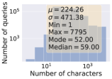
(a)

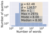
(b)

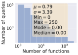
(c)

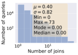
(d)

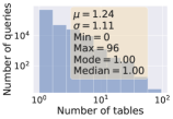
(e)

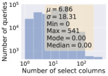
(f)

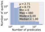
(g)

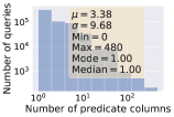
(h)

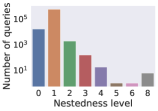
(i)

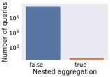
(j)

Figure 3. Structural properties of SDSS query statements.

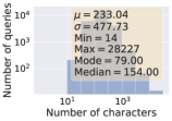
(a)

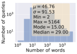
(b)

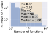
(c)

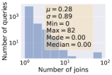
(d)

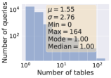
(e)

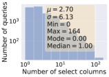
(f)

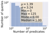
(g)

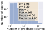
(h)

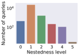
(i)

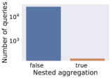
(j)

Figure 4. Structural properties of SQLShare query statements. Most plots are on log-log scale, due to the wide data range.

4.3.1. Query Statement Analysis

We analyze the query statement properties to understand the type of queries posed and their syntactic properties and statistics. Regarding the query statement types, SELECT statements comprise approximately 96.5% and approximately 98% of statements on SDSS and SQLShare, respectively. The remaining 3.36% (21540) and 2.02% (544) of statements on SDSS and SQLShare, correspond to types such as EXECUTE, CREATE, DROP, UPDATE, ALTER, and various combinations like DELETE — UPDATE — INSERT.

We used the ANTLR parser (Parr, 2013) to generate the Abstract Syntax Trees (AST) of query statements and extract 10 syntactic properties:

1. number of characters: the number of characters in a query.

2. number of words: the number of words in a query (digits are replaced with the $<$DIGIT$>$ token).

3. number of functions: the number of function calls.

4. number of joins: the number of join operators.

5. number of unique table names: the number of unique table names in the query.

6. number of selected columns: the number of selected columns in the query.

7. number of predicates: the number of predicates (logical conditions, e.g., s.flags_s=0) used in a query.

8. number of predicate table names: the number of table names in the predicates.

9. nestedness level: the level of nestedness.

10. nested aggregation: it is true if nested queries involve aggregation and false otherwise.

Example 4.1.

The query in Figure 5 has the following syntactic properties:

1. number of functions ​=$2$ (dbo.fGetURLExpid and min),

2. number of unique table names ​=$2$ (SpecPhoto and PhotoObj),

3. number of selected columns ​=$3$ (objid, modelmag_u, modelmag_g),

4. number of predicates ​=$5$ (1 in the main query and $4$ in the sub-query including the predicate for the inner join operator),

5. number of predicate table names ​=$7$ ($7$ logical conditions),

6. nestedness level ​=$1$,

7. nested aggregation ​=true (the nestedness involves min).

⬇

SELECT dbo.fGetURLExpid(objid)

FROM SpecPhoto

WHERE modelmag_u-modelmag_g =

(SELECT min(modelmag_u-modelmag_g)

FROM SpecPhoto AS s INNER JOIN PhotoObj AS p

ON s.objid=p.objid

WHERE (s.flags_g=0 OR p.psfmagerr_g<=0.2 AND

p.psfmagerr_u<=0.2)

Figure 5. A sample query from SDSS

Statistics of the syntactic properties of SDSS statements are shown in Figure 3 (cf. Figure 4 for SQLShare). Figures 3a and  3b plot the distribution of characters and words for SDSS. The maximum number of characters and words is 7,795 and 2,975 (5164 and 28227 for SQLShare), respectively. Around $30\%$ of the queries have more than 62 characters, and more than 224 words (whcih are the corresponding distribution means). Figures 3c- 3i report key structural metrics such as the number of joins and number of predicates for SDSS (cf. Figures 4c- 4i for SQLShare) Approximately $5.91\%$ ($1.68\%$) of the queries in SDSS (SQLShare) have at least one join operator, $14.01\%$ ($29.74\%$) of the queries in SDSS (SQLShare) access more than one table, $0.34\%$ ($7.88\%$) of the queries in SDSS (SQLShare) are nested queries, and $0.03\%$ ($0.71\%$) are nested queries with aggregation. Note that the small percentage of nested queries still corresponds to a considerable number of queries ($2,112$ for SDSS and $2,107$ for SQLShare).

Our analysis of the syntax of queries in SDSS and SQLShare shows that these workloads have queries of various complexity w.r.t. the syntactic properties that we studied. Comparing the syntactic properties of the statements in SDSS with those in SQLShare, we observe that while queries are typically longer in SQLShare, the mean number of predicates in the where clause for SDSS is approximately four times that of SQLShare (Figure 4g vs. Figure 4g). Although SQLShare queries access more tables on average (as depicted by a higher mean value and maximum in Figure 3e vs. Figure 4e), SDSS queries perform more joins on average (as depicted by a higher mean value and maximum Figure 3d vs. Figure 4d). Finally, SQLShare’s queries are more complex in both nestedness and aggregation.

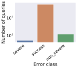
(a) SDSS

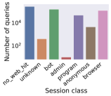
(b) SDSS

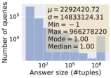
(c) SDSS

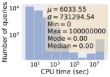
(d) SDSS

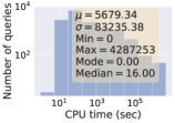
(e) SQLShare

Figure 6. Label distributions for classification (Figures 6a and 6b) and regression problems (Figures 6c-6e).

4.3.2. Label Analysis

Figures 6a and 6b show the label distributions of the classification problems for SDSS. As shown in Figure 6a, the error classes are imbalanced; 97.22% of the queries ran without an error (success), while 1.93% had non_severe errors, and 0.85% had severe errors. Figure 6b shows that session classes are also imbalanced, e.g., program and bot comprise 7.93% and 25.98% of the workload, respectively. Note, a simple model that only predicts the majority class (e.g. success in error classification) will achieve a high accuracy. We address this issue in our evaluations by separately calculating the per-class F-measure.

Figures 6c-6e show the label distributions for regression problems. Figure 6c shows SDSS answer size distribution, which ranges from a minimum of -1 (the query did not run due to an error) to a maximum value of 966,278,220 tuples. Despite the wide range of values, the data is concentrated around smaller values with a median of 1, i.e., half of the queries either do not run, return no answer, or return only one answer. Figure 6d shows the CPU time distribution on SDSS. The time ranges between $0$ and $10^{8}$ seconds with the majority of queries taking little CPU time. Figure 6e shows the CPU time distribution in SQLShare ranges approximately between $0$ and $4*10^{6}$ seconds.

4.4. Workload Analysis Implications

4.4.1. Model Selection and Train Loss Functions

Our query facilitation problems in Definition 4 can broadly be categorized as supervised classification and regression problems. Text classification in NLP is a closely related area. Traditional NLP models, work in two stages: a feature extraction phase, where input features are hand-engineered, and a prediction phase. As shown in Figure 3, queries range in complexity and extracting an adequate set of features can be challenging. Neural network architectures can learn features automatically. They combine the feature extraction and prediction stages in a joint training task, which allows them to develop features and representations for the task (Conneau et al., 2016). LSTMs are a type of recurrent neural network (RNNs), and are one of the dominant models for text classification. They treat text as sequential inputs and try to preserve long-term dependencies between tokens. However, query statements are long (Figures 3a and 3b), and this property can negatively affect the performance of LSTMs. As an alternative, we assess CNNs, which are feed-forward networks. Rather than preserving long-term dependencies, CNNs automatically identify local patterns (i.e., n-grams) in the input and preserve them in their feature representations. For NLP tasks, CNNs are known to be competitive with several more sophisticated architectures (e.g., LSTMs) and are easier to train and interpret (Bai et al., 2018; Yin et al., 2017).

Moreover, we observe that SQL queries (and code in general) often contain mathematical expressions consisting of numbers and operators. These expressions significantly affect query properties like query answer size or CPU time (Ganapathi et al., 2009). It is beneficial to retain relevant information in the representation of queries. However, the set of variable names and digits used in code snippets is unbounded, and there are many rare words. For word-levels models, this leads to the unbounded or open vocabulary problem, which creates practical issues when learning representations in machine learning (Kim et al., 2016). We apply the models in Section 5, at both character and word level. For the latter, we replace the digits with a $<$DIGIT$>$ token to control for the vocabulary size.

Regarding the train loss functions, we observe that the error class and session class labels are imbalanced (Figures 6a and 6b). For some applications, like bot detection, models that perform accurately on certain classes may be required. Typically, application-dependant assumptions are enforced by either re-sampling the data, or using weighted loss functions during training of models. Because our work does not focus on specific applications (e.g., bot detection), we treat all classes equally and use an unweighted cross entropy loss function for training the classification models in Section 5. Our evaluation (Section 6), however, considers this class imbalance where we analyze performance w.r.t. each class.

The regression labels have a wide range of values and are highly skewed, with the majority of queries concentrated around small values (Figures 6c- 6e). To prevent the models from being too sensitive to queries with a large label value (outliers), we perform two steps. We apply a logarithmic transformation to the values of these labels $y^{\prime}_{i}=\ln(y_{i}+\epsilon-\min(\bm{y}))$, where $y_{i}$ is the label of query $i$, and $\bm{y}$ is a vector representing the labels (answer size or CPU time) of all queries, and $y^{\prime}_{i}$ is the log-transformed value. When $y_{i}=\min(\bm{y})$, $\epsilon>0$ prevents the input of the $\ln(.)$ function from being zero. We set $\epsilon=1$ to make the transformation non-negative. We use the log-transformed values of CPU time and answer size as the labels of queries in regression problems. Moreover, to ensure that the regression models are robust to outliers in the data, during training we use the well-known Huber loss (Huber et al., 1964), which is a hybrid between $l_{2}$-norm for small residuals and $l_{1}$-norm for large residuals.

4.4.2. Model Evaluation

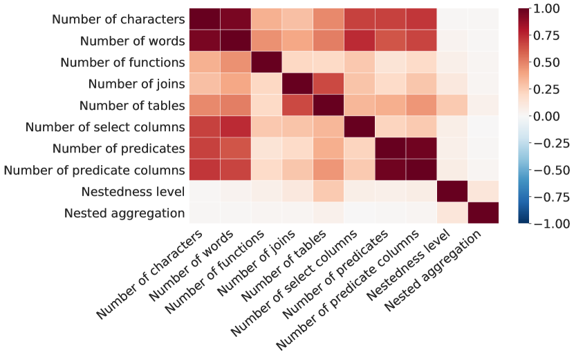
(a) SDSS

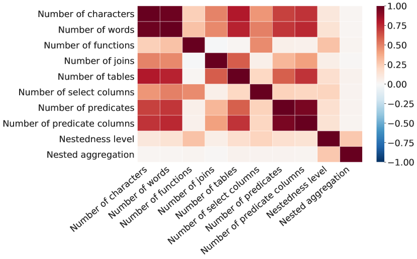
(b) SQLShare

Figure 7. Correlation matrix of strutural properties in Figures 3 and Figures 4.

In our work, we want to help end users write queries. This is particularly important in settings where query statements are complex and for users who have little experience. Therefore, we need to assess model performance on complex query statements. However, statement complexity information is not included explicitly in the data. To effectively assess feasibility of complex queries, we must define both a notion of query statement complexity and a proxy measure that captures it.

Similar to (Jain et al., 2016), we want a proxy metric for complexity that reflects the cognitive effort required to write the query statement. Metrics based on query run time (Ganapathi et al., 2009) are not adequate in this context. The run time depends on factors like the load of the database or the size of data selected, which are not relevant to the cognitive effort of the user, e.g., a simple query that selects all rows of a large table can have a long running time. In (Jain et al., 2016), query complexity is defined in terms of the query’s ASCII length and the number of distinct operators in the query execution plan. However, we do not assume access to the database instance or execution plan. The ASCII length, on the other hand, might not be a sufficient proxy for complexity, e.g., when a query has a simple structure with similar operations repeated many times. Additional syntactic properties may be required.

However, it is not clear which set of syntactic properties capture a meaningful notion of statement complexity. Figure 7 shows the correlation matrix for the syntactic properties in Figure 3 for SDSS. We observe some properties are positively and linearly correlated with other types of properties, and hence indicative of them. For example, the number of characters is linearly correlated with the number of words, the number of predicate table names, the number of predicates, and the number of selected columns So the latter properties are redundant since the number of characters is indicative of them. But number of characters is not positively correlated with properties like nested aggregation and nestedness level and may not capture those complexities. As another example, the number of joins is only linearly correlated with the number of unique table names. We observed similar patterns for SQLShare in Figure 7b.

Overall, these observations suggest that a subset of syntactic properties might be required to capture the full range of potential query complexities. Based on the query statement feature correlations shown in Figure 7, we chose a subset of five syntactic properties for the qualitative analysis in Section 6.3.3. These include the number of characters, the number of functions, the number of joins, the nestedness level, and the nested aggregation indicator.

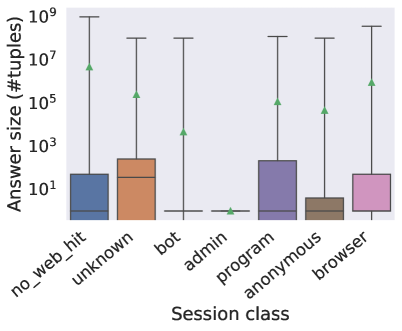
(a) Answer size

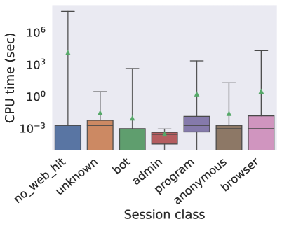
(b) CPU time

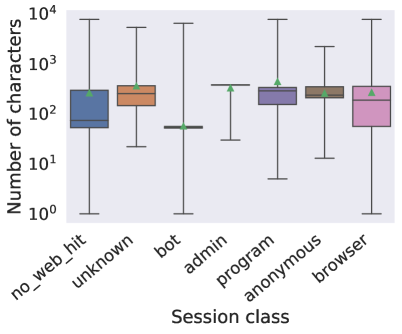
(c) Number of characters

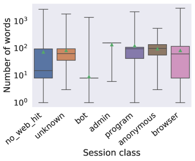
(d) Number of words

Figure 8. SDSS analysis by session class. The top and bottom of each box represent the first and third quartiles of the class data distribution. The horizontal line in each box is the median, the mean is a green triangle.

One viable assumption may be that different classes of users write queries with different complexity levels. For example, bot queries may use linear predicates in the where clause, while queries via browser may be more complex. Thus, session class, if available, can be an indirect proxy for query complexity. We examined the SDSS queries and broke down several of their properties by session class.Figure 8a plots the distribution of the answer size for each session class. The no_web_hit and browser classes have similar distributions, with the latter having slightly smaller values (likely due to the limitations for queries posed via the web-based interface). In Figure 8b the distribution of the CPU time for each session class is shown. Queries in the no_web_hit class have a wider range of values. Figures 8d and 8c show the query size distributions by session class. Overall, queries from no_web_hit and browser classes have similar distributions at both the character and word level. These figures suggest that queries in the no_web_hit and browser class are more complex. The drawback is that session class information may not always be available, e.g., SQLShare workload does not include it.

5. Methods

Based on our analysis in Section 4.4.1, we extend three models from the NLP domain and benchmark their performance for our problems. In Section 5.1 we describe a traditional model. In Section 5.2 we describe a three-layer LSTM model and in Section 5.3 we describe a shallow CNN. Details of the models are in Appendix A.

5.1. Traditional Model

Traditional machine learning models work in two stages: a feature extraction phase and a prediction phase. For the feature extraction phase, Bag-of-ngrams and its TFIDF (term-frequency inverse-document-frequency) are commonly used in NLP applications. For the Bag-of-ngrams, we select the most frequent $n$-grams (up to 5-grams) from the training set. These features comprise the domain vocabulary $V$ with size $v$. Thus, this representation maps each query to a $v$-dimensional vector obtained by computing the sum of the one-hot representation of the $n$-grams that appear in the query. Next, we compute the TFIDF weight of each token $t_{i}$ in the $v$-dimensional representation of query $Q$ w.r.t. the collection of queries $\mathcal{Q}$. In particular, the weight of token $t_{i}$ is computed using $\textit{TFIDF}(t_{i},Q,\mathcal{Q})=\textit{TF}(t_{i},Q)\times\textit{IDF}(t_{i},\mathcal{Q})$. Here $TF(t_{i},Q)$ is the normalized frequency of $t_{i}$ in $Q$. The normalization prevents bias towards longer queries. The $\textit{IDF}(t_{i},\mathcal{Q})$ component describes the discriminative power of $t_{i}$ in $\mathcal{Q}$ and helps to control for the fact that some tokens are generally more common than other tokens. It can be computed by $\log{\frac{|\mathcal{Q}|}{1+|\{Q\in\mathcal{Q},t_{i}\in Q\}|}}$, where the denominator is the number of queries in $\mathcal{Q}$ that contain $t_{i}$. The TFIDF value increases proportionally to the frequency of a token in a query but is counterbalanced by the frequency of the term in the collection. As a token appears in more queries, the ratio inside the logarithm approaches $1$, bringing the IDF and TFIDF closer to 0.

We then apply a prediction model given this fixed $v$-dimensional feature vector. For classification problems, we apply the multinomial logistic regression model. For regression problems, we use Huber loss (Huber et al., 1964). We optimize the parameters of the prediction model using scikit-learn (Pedregosa et al., 2011).

5.2. Three-layer LSTM

Long-Short Term Memory (LSTM) is a type of recurrent neural network (RNN) (Zaremba and Sutskever, 2014). RNNs can process sequential inputs of arbitrary length. Figure 9 shows a standard RNN unit. It works by reading the input sequence one token at a time from left to right.At every step $i$, a hidden state $\bm{h}_{i}\in\mathbb{R}^{k}$ is emitted, which is a semantic representation of the sequence of tokens observed so far. Specifically, $\bm{h}_{i}$ is produced using the recurrent equation $\bm{h}_{i}=f(\bm{W}\bm{x}_{i}+\bm{U}\bm{h}_{i-1}+\bm{b})$ where $\bm{x}_{i}\in\mathbb{R}^{d}$ is the distributed representation of the input token $q_{i}$, and $\bm{h}_{i-1}\in\mathbb{R}^{k}$ is the hidden state at $i-1$. The parameters of this RNN unit include weight matrices $\bm{W}$ and $\bm{U}$, and a bias vector $\bm{b}$. $f(.)$ is a point-wise non-linear activation function, such as the Sigmoid or Rectified Linear unit (Relu) (Goodfellow et al., 2016).

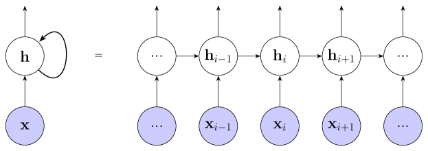
Figure 9. An RNN network with hidden-to-hidden recurrent connections.

Standard RNNs suffer from the vanishing gradient problem. In particular, during training, the gradient vector can grow or decay exponentially (Tai et al., 2015; Goodfellow et al., 2016). LSTMs are a more effective variant of RNNs. They are equipped with a memory cell $\bm{c}\in\mathbb{R}^{k}$, which helps preserve the long-term dependencies better than standard RNNs. The LSTM unit (Zaremba and Sutskever, 2014) has a hidden state $\bm{h}_{i}$ that is a partial view of the unit’s memory cell. The unit is equipped with additional parameters and machinery to produce $\bm{h}_{i}$ from $\bm{c}_{i-1}$ (memory cell at step $i$), $\bm{x}_{i}$, and $\bm{h}_{i-1}$(details in Appendix A.2).

Since well-known RNN architectures do not exist for our problems, we explore those used in similar domains. Deep architectures consisting of many layers are often developed to learn hierarchical representations for the input and to learn non-linear functions of the input (Conneau et al., 2016). However, increasing the number of layers and units increases the number of parameters to learn, and training time increases substantially.

A two-layer character-level LSTM architecture was used to predict program execution in (Zaremba and Sutskever, 2014). Motivated by their success, we use a three-layered LSTM model. We use the output of the last layer as the query vector representation. For classification problems, we apply the softmax operation to generate the output probability distribution. Similar to the traditional models, we use the cross-entropy loss for classification problems. For regression problems, we pass the the vector through a linear unit and use Huber loss. To optimize the network, we examined both Adam and AdaMax (Kingma and Ba, 2014) which are gradient-based optimization techniques that are well suited for problems with large data and many parameters. We found the latter performed better.

5.3. Shallow CNN

Convolutional Neural Networks (CNNs) are feed-forward neural networks that process data with grid-like topology, e.g., a sequence of concatenated distributed representations of tokens in NLP. Their application in NLP enables the model to extract the most important n-gram features from the input and create a semantic representation. As a result, long-term dependencies may not be preserved and token order information is preserved locally. CNNs, however, have comparable performance to RNNs, they are easier to train, and are also parallelizable (Young et al., 2018; Bai et al., 2018; Yin et al., 2017).

Figure 10. 1D convolution operation with input $\bm{x}_{1:n}$ and kernel $\bm{w}$. The output $\bm{p}=\bm{x}_{1:n}*\bm{w}$ is produced by sliding $\bm{w}$ over $\bm{x}_{1:n}$ and computing the dot product.

Each layer in a CNN consists of three stages (Goodfellow et al., 2016): a convolution stage, a detection stage, and a pooling stage. We explain each of stages based on a 1D convolution operation, although higher dimensions are also possible.

The convolution stage applies several convolution operations. A convolution operator has two operands: a multidimensional array of weights, called the kernel, and a multidimensional array of input data. Convolving the input with the kernel consists of sliding the kernel over all possible windows of the input. At every position $j$, a linear activation $p_{j}$ is obtained by computing the dot product between the kernel entries and local regions of the input. Figure 10 shows an example of a 1D convolution operation. Let $\oplus$ denote the concatenation operation, and $\bm{x}_{1:n}=\bm{x}_{1}\oplus\bm{x}_{2}\oplus\dots\oplus\bm{x}_{n}$ denote the concatenated distributed representations $\bm{x}_{i}$ in an input query (stacked length-wise as a long column). Let $\bm{x}_{j:j+m-1}$ represent a window of $m$ words and $\bm{w}\in\mathbb{R}^{m}$ denote a kernel. The dot product of $\bm{w}$ and each $m$-gram in the sequence is computed to obtain $p_{j}=\bm{w}^{T}\bm{x}_{j:j+m-1}+b$ where $b\in\mathbb{R}$ is a bias term. By sliding the kernel over all possible windows of the input, we obtain a sequence $\bm{p}\in\mathbb{R}^{n-m+1}$ ($b=0$ in Figure 10). Note, in the convolution stage, several kernels with varying window sizes may be convolved with the data to produce different linear sequences. In the detector stage, the linear sequence $\bm{p}$ is run through a non-linear activation function. This results in a sequence of non-linear activations called the activation map $\bm{a}=f(\bm{p})$, where $\bm{a}\in\mathbb{R}^{n-m+1}$ and $f(.)$ is a non-linear activation function, e.g., Relu. In the pooling stage a pooling operation is applied to the activation map to summarize its values which also enables the model to handle inputs of varying size. For example, the max-pooling function returns the maximum, i.e.,  $g=\max\{\bm{a}\}$.

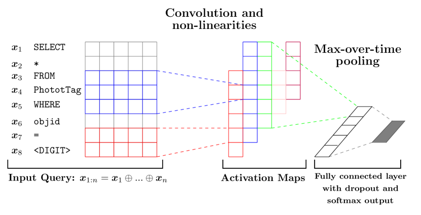
Figure 11. 1-layer CNN, adapted from (Kim, 2014).

Figure 11 shows the shallow CNN architecture in (Kim, 2014), which we adapt for our application. The input query $\bm{x}_{1:n}$ and convolution operations are shown in 2D for easier presentation. In the convolution stage, several filters of varying window size $m\in\{3,4,5\}$ are applied, and the resulting sequence $\bm{p}_{1},\bm{p}_{2},...$ is passed through a Relu function to generate activations $\bm{a}_{1},\bm{a}_{2},...$ . Different size sequence inputs and kernels result in activation maps of different sizes. To deal with variable length of the input and also obtain the most important feature, a max pooling operation is applied to obtain a single feature per kernel, $g=\max\{\bm{a}\}$. The resulting features for all kernels are concatenated to produce a fixed size vector $\bm{g}\in\mathbb{R}^{K}$, where $K$ is the number of kernels. This output is used to create a fully connected layer, followed by a dropout layer.

We tried changing the architecture by increasing the number of kernels and the window size but did not obtain significant improvements. Similar to the other models, for classification problems we apply the softmax operation to generate the output probability distribution. We use the cross-entropy loss for classification problems. For regression problems, we pass the the vector through a linear unit and use Huber loss to learn the parameters. We used AdaMax as the optimizer.

6. Empirical Evaluation

We evaluate the performance of models in Section 5 on the four query facilitation problems, considering two aspects: (1) the different query facilitation problem settings and (2) the query statement complexity (described in Section 4.4.2).

6.1. Setup

Data split. For Homogeneous Instance, we used our extracted SDSS workload. For Homogeneous Schema, we used SQLShare. In both settings, we randomly split the queries. For Heterogeneous Schema, we used SQLShare and randomly split the data based on users, so as to decrease the likelihood of data sharing. Table 1 summarizes our datasets.

	Homogeneous	Homogeneous	Heterogeneous
	Instance	Schema	Schema
Total	618,053	26,728	26,728
Train	494,443	21,382	22,068
Valid.	61,805	2,673	1,893
Test	61,805	2,673	2,767

Table 1. The number of queries and data split in SDSS (Homogeneous Instance), and SQLShare (Homogeneous Schema and Heterogeneous Schema).

Methods compared. We compare the models in Section 5, where character-level model names begin with c and word-levels models with w. The traditional models are ctfidf and wtfidf. The 3-layer LSTM models are clstm and wlstm. The CNN models are ccnn and wcnn. For each prediction task, we also include a simple baseline. For classification problems, mfreq predicts the most frequent label, i.e., it predicts success for error classification, and no_web_hit for session class prediction. For regression problems, median predicts the median of the corresponding train distribution, i.e., the median of train answer size distribution is 1.099, and the median of the train CPU time distribution is 0. Following (Li et al., 2012; Ganapathi et al., 2009; Akdere et al., 2012) we report results for an opt model which uses linear regression to predict CPU time from the query optimizer estimates cost estimates.

Hyper-parameter tuning. We tune the hyper-parameters based on Homogeneous Instance (SDSS). To keep this problem tractable, we restrict the set of hyper-parameters of each model and choose the best set of hyper-parameters based on performance on the validation set. We fixed the learning rate 1e-3, batch size to 16, token embedding size to $100$, and weight decay set to 0 For clstm and wlstm, we tested the number of hidden dimensions in $\{150,300\}$ and clipping rate in $\{0.25,0\}$. For ccnn and wcnn, we tested number of kernels in $\{100,250\}$, drop out in $\{0.5,0\}$, and clipping rate in $\{0.25,0\}$. We report results for the best performing model and also use the model in Homogeneous Schema and Heterogeneous Schema settings.

Performance metrics. For the classification problems we report the test average loss computed according to cross entropy (loss)Eq. A.3 . We also report Accuracy, which is the number of correct predictions divided by the total number of predictions. Due to the class imbalance for both error and session classification, for every class $C$, we report the per class F-measure computed by $\text{F}_{C}=\frac{2.\text{Precision}_{C}.\text{Recall}_{C}}{\text{Precision}_{C}+\text{Recall}_{C}}$. $\text{Precision}_{C}$ is the number of correct predictions for class $C$ divided by the total number predictions for class $C$. $\text{Recall}_{C}$ is the number of correct predictions for class $C$ divided by the total number queries in class $C$. For the regression problems we report the test average loss computed according to Huber loss(Eq. A.1) . We also report Mean Square Error (MSE) computed as $\text{MSE}=\frac{1}{m}\sum_{i}^{m}(y^{\prime}_{i}-\hat{y}_{i})^{2}$, where $y^{\prime}_{i}$ is the log-transformed label (CPU time or answer size) of query $i$, and $\hat{y}_{i}$ is the predicted value. We also use qerror which measures the quality of estimates (Leis et al., 2015). The qerror of a query $Q_{i}$ is $\textit{q-error}_{i}=\max(\frac{y_{i}}{\hat{y_{i}}},\frac{\hat{y_{i}}}{y_{i}})$.

6.2. Model Performance

		Error Classification						CPU Time		Answer Size
Model	$v$	$p$	Accuracy	Fsevere	Fsuccess	Fnon_severe	Loss	$p$	Loss	$p$	Loss
baseline	-	-	0.9730	0.0000	0.9863	0.0000	0.5951	-	0.0675	-	1.6357
ctfidf	500000	1500000	0.9778	0.7131	0.9888	0.0053	0.5860	500000	0.0668	500000	1.0400
ccnn	159	17403	0.9797	0.7961	0.9897	0.1669	0.1106	16801	0.0471	16801	0.7517
clstm	159	1944003	0.9786	0.6922	0.9893	0.2206	0.0830	1943401	0.0452	529651	0.7678
wtfidf	500000	1500000	0.9773	0.6546	0.9885	0.0620	0.5836	500000	0.0668	500000	1.0922
wcnn	85942	8597953	0.9790	0.7441	0.9894	0.2006	0.1006	8595101	0.0441	8595101	0.8472
wlstm	85942	10522303	0.9776	0.6971	0.9887	0.0018	0.0691	10521701	0.0443	9107951	0.8256

Table 2. Query error classification (left), CPU time (middle), and answer size (right) prediction in Homogeneous Instance (SDSS). Here $v$ is #tokens in the vocabulary, $p$ is #model parameters, Loss is the average test loss (lower loss is better). baseline is median in the regression problems and mfreq in the classification problem. In the classification problem, F_C is the F-measure of class C. The #samples of each class in the test set are: severe $=533$, success $=60138$, non_severe $=1134$.

6.2.1. Homogeneous Instance

Table 6.2 (left) shows the error classification results. The mfreq baseline achieves a high $\text{F}_{\tt success}$ but performs poorly w.r.t. other classes. All other models improve upon this baseline. The ccnn model obtains a high $\text{F}_{\tt severe}=0.7961$ and has the highest test accuracy. Table 6.2 (middle) shows results for CPU time prediction. The wcnn model obtains the lowest test loss, followed closely by the wlstm model. Table 6.2 (right) shows results for answer size prediction. The ccnn model obtains the lowest test loss, followed closely by the clstm model. In Section 6.3.1 we assess both problems w.r.t. MSE values. Table 6.2 shows results for session classification. Again the mfreq baseline achieves a high $\text{F}_{{\tt no\_web\_hit}}$ (the majority class) but under-performs all other models w.r.t. other classes. The highest test accuracy is obtained by the ctfidf model, which outperforms other models in the F-measure of individual classes, except for $\text{F}_{{\tt unknown}}$ which is 0. $\text{F}_{{\tt admin}}$ is 0 since admin only has 2 queries in the test set.

Table 6.2 shows the qerror of the answer size predictions of 62K test queries in SDSS. The percentage of queries that have at most the reported qerror is shown, e.g.,  the qerror of $75\%$ of the test queries is less than $2.38$ for clstm. Intuitively, qerror for answer size is the factor by which an estimate differs from the true answer size. We observe ccnn and clstm have lowest qerrors. Note, all models perform well for $50\%$ of the queries and the main comparison is for the other $50\%$ of the queries for which prediction is more difficult.

Table 3. Answer size prediction qerror (SDSS).

Table 4. Query Session classification in Homogeneous Instance (SDSS). The #examples in the test set for each class is: no_web_hit $=27677$, unknown $=42$, bot $=16148$, program $=4882$, anonymous $=467$, browser $=12587$.

6.2.2. Homogeneous Schema

Table 6.2 reports performance for CPU time prediction in Homogeneous Schema. The ccnn model outperforms other models. Compared to Homogeneous Instance, the overall loss value is higher for all models in Homogeneous Schema. This is because the latter poses an additional challenge where the distribution of the queries in individual database instances is different, and to get accuracy compared to Homogeneous Instance, we need to increase model capacity (e.g., add more layers in the architecture). Moreover, observe that the opt model, that is based on the query optimizer cost model, is closer to median in it’s error. Our qerror analysis for 2,674 test queries in SQLShare shows ccnn performs better across different percentiles. For $50\%$ and $75\%$ of the queries, qerror is less than $1.94$ and $27$, resp (Table 6.2).

Table 5. Query CPU time prediction (SQLShare)

6.2.3. Heterogeneous Schema

Table 6.2 reports performance for CPU time prediction in Heterogeneous Schema. Similar to Homogeneous Schema, the ccnn model outperforms others. However, compared to Homogeneous Instance and Homogeneous Schema, the loss value achieved by all models is higher. This is expected since the data is extracted from databases with different schemata, which makes it more challenging for the models to predict, i.e., the train and test sample distributions are different. For opt, prediction is more difficult, too. As explained in (Akdere et al., 2012), the query optimizer cost model assumes I/O is most time consuming, even though certain computations (e.g., nested aggregates over numeric types) are performed in memory. Moreover, a non-linear regression model may improve performance of opt. Our qerror analysis shown in Table 6.2, shows ccnn performs better across different percentiles in Heterogeneous Schema. For $30\%$ of the queries, qerror is less than $34$. The substantial qerror increase means prediction is harder in Heterogeneous Schema.

Table 6. CPU time prediction qerror (SQLShare, Homogeneous Schema).

Table 7. CPU time prediction qerror (SQLShare, Heterogeneous Schema).

6.2.4. Discussion

We found the following: (1) Character-level models (ccnn and ctfidf) obtain the best performance for all problems except CPU time prediction in Homogeneous Instance, where word-level models (wcnn and wlstm) obtained the lowest test loss and MSE. Intuitively, as the problem heterogeneity increases, the number of rare words increases, making it difficult to learn word-level patterns. In Homogeneous Instance setting, however, queries have more words in common (e.g., table names and SQL keywords), and the models can learn the underlying distributions better. (2) Overall, CNN and LSTM architectures outperform others on all problems except session classification, where ctfidf obtains better results in predicting several classes. The frequency of the classes (see Table 6.2) shows that ctfidf performs better for majority classes (e.g., no_web_hit and bot); and CNN and LSTM beat ctfidf in non-frequent classes (e.g., unknown and program) where prediction is more difficult. In addition, ccnn achieves almost the same overall accuracy with much fewer parameters ($16801$ vs $500000$). The neural networks learn features w.r.t. task, but ctfidf and wtfidf are limited to pre-determined features. (3) Regarding generalization of a single model under various settings, ccnn identifies local sequential character patterns which help it learn the underlying data distribution better.

6.3. Detailed Qualitative Analysis

6.3.1. Performance by Session Class

We perform a finer-level of analysis and use the session class information as a proxy for complexity under the Homogeneous Instance setting. We analyze CPU time prediction performance in Figure 12a and answer size prediction in Figure 12b. The figures show MSE of prediction by session class for each model. The MSE trends show that predicting CPU time for no_web_hit, program, and browser is more difficult. Moreover, the simple baseline median under-performs all models across all sessions. Interestingly, ctfidf and wtfidf perform similarly to median for CPU time prediction, and under-perform all other models for Answer size prediction. This shows the neural network models perform better on complex session classes.

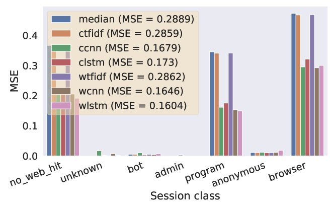
(a) CPU time prediction by session class.

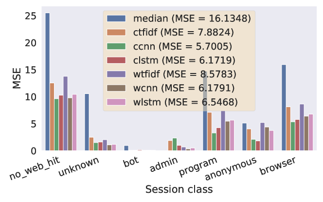
(b) Answer size prediction by session class.

Figure 12. MSE of regression problems by session class in Homogeneous Instance (SDSS). In 12a, ctfidf, wtfidf, are similar to median baseline while they outperform it in 12b. The neural network models outperform all baselines.

6.3.2. Performance by Structural Properties

Figures 13a-13e analyse error of answer size prediction for varying structural properties under Homogeneous Instance. As expected, error increases for more complex queries (with larger number of characters, number of functions, number of joins and nestedness level). The decrease of error in the middle and end of the graphs in Figures 13a-13c is due to fewer answers for the corresponding queries, which makes prediction easier for all the models (including median, which supports this claim).

Figure 14 shows MSE for CPU time predication. For all models, error increases from Homogeneous Instance to Homogeneous Schema to Heterogeneous Schema, because the problem setting heterogeneity makes prediction more difficult. Figure 14 also shows the MSE of ccnn increases for more complex queries. Again, the unexpected decrease in MSE of queries with high nestedness (see nestedness level ​=$3,4$ in Figures 14b, 14d and 14f) is due to better prediction for the few queries with small CPU time.

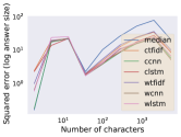
(a)

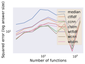
(b)

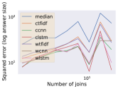
(c)

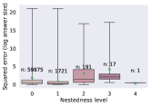
(d) error analysis for ccnn

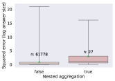
(e) error analysis for ccnn

Figure 13. Error analysis of answer size prediction on SDSS (Homogeneous Instance). Considering session class 9.a, and considering structural properties 9.b-9.e. MSE of each model is reported in legend of 9.a.

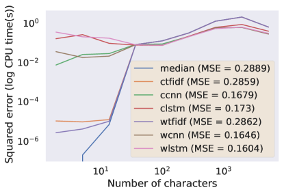
(a) Homogeneous Instance

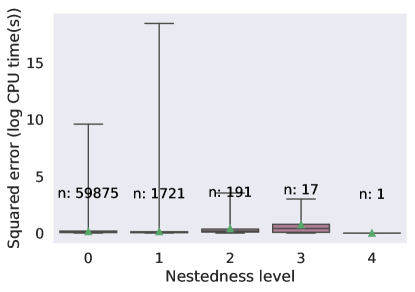
(b) Homogeneous Instance

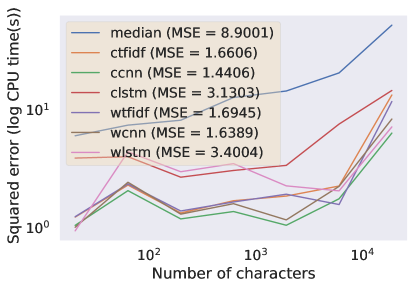
(c) Homogeneous Schema

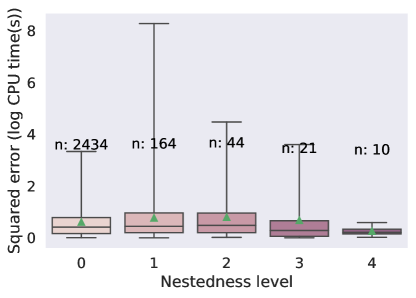
(d) Homogeneous Schema

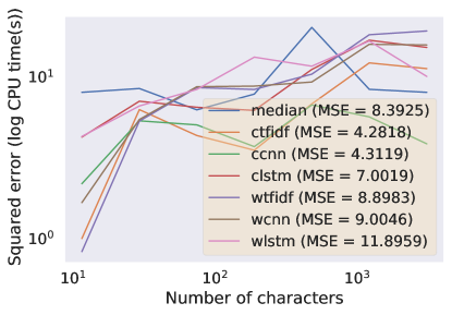
(e) Heterogeneous Schema

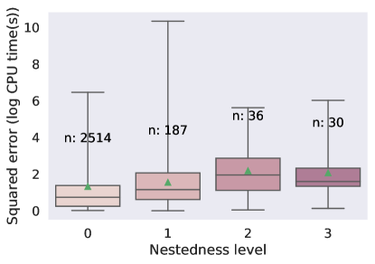
(f) Heterogeneous Schema

Figure 14. Error analysis of CPU time prediction by number of characters (left). Error analysis of CPU time prediction for ccnn by nestedness level (right).

6.3.3. Case Study

We study performance for two sample queries with different structural properties. $Q_{1}$ in Figure 15 is a large query (number of characters =$1,247$ and number of words =$376$) that joins three large tables (e.g., Specobj and Photoobj contain $4,311,571$ and $794,328,715$ rows, respectively), selects 49 columns in the answer, and calls 3 functions. The query is from the browser and ran successfully (error class: success) with CPU time of $105.37$ sec and returned $304$ answers. Comparing ccnn and clstm, the former predicts $116.40$ sec for CPU time while clstm’s estimation is $980$ sec. The query length makes it hard for clstm to capture the long-term dependencies, whereas ccnn detects local patterns and combines them globally to make a better prediction.

$Q_{2}$ in Figure 16, is shorter than $Q_{1}$ (number of characters ​=$645$ and number of words ​=$181$), but it is more complex (nestedness level ​=$3$, number of functions ​=$5$, and number of predicates ​=$11$). The query runs instantly since it accesses tables (Jobs, Users, Status and Servers) with fewer rows. Its answer size is $27$ rows. The CPU time prediction of ccnn, wcnn and clstm are $1.00$ sec, $1.28$ sec and $1.01$ sec, respectively. Their answer size predictions are $45$, $46$ and $49$. For $Q_{2}$ all 3 models perform fairly well. The small CPU time and the answer size of $Q_{2}$ compared to $Q_{1}$, contributes to more accurate predictions (due to the logarithmic label transformation and Huber loss (cf. Section 4.4.1)). $Q_{2}$ is shorter in length compared to $Q_{1}$, which makes it easier for clstm to make predictions.

6.3.4. Discussion

Using session information, CPU time and answer size prediction were more difficult for no_web_hit, program, and browser sessions, for all models. This is because queries in these classes are more complex compared to other classes (see Figure 8) and are likely issued by humans. Our evaluation by structural properties showed that predicting labels is more difficult for complex queries (e.g. with large number of characters, number of functions, number of joins), and in settings where data is from heterogeneous sources. Word-level models suffer from many rare tokens in heterogeneous settings, and do not generalize well. Among the character-level models, clstm is sensitive to the query length and is outperformed by ccnn as statement complexity increases.

⬇

SELECT q.name AS qname,

dbo.fDistanceArcMinEq(q.ra,q.dec,p.ra,p.dec), ...

FROM SpecObj AS s,

SDSSSQL010.MYDB_670681563.test.QSOQuery1_DR5 AS q, PhotoObj AS p

WHERE ((s.bestobjid=p.objid) AND (s.ra BETWEEN 185 AND 190) AND ...) ORDER BY q.ra

Figure 15. Sample query $Q_{1}$

⬇

SELECT j.target,cast(j.estimate AS varchar) AS queue,...

FROM Jobs j,Users u,Status s,

(SELECT DISTINCT target,queue FROM Servers s1

WHERE s1.name NOT IN

(SELECT name FROM Servers s,

(SELECT target,min(queue) AS queue

FROM Servers GROUP BY target) AS a

WHERE a.target=s.target)) b

WHERE j.outputtype LIKE '%QUERY%' AND ...

Figure 16. Sample query $Q_{2}$

7. Related Work

Deep learning, Machine Learning, and NLP. RNNs and CNNs are dominant in many text applications (Conneau et al., 2016). Character-level LSTMs were used for program execution in (Zaremba and Sutskever, 2014). In (Kim, 2014), a one-layer word-level CNN model outperformed tree-structured models that use syntactic parse trees as their input, for text categorization. Deep character-level CNN models (Zhang et al., 2015; Conneau et al., 2016; Johnson and Zhang, 2016a) outperformed shallow word-level CNNs (Johnson and Zhang, 2016a). Although shallow word-level models have more parameters and need more storage, their computations are faster. Subsequently, deep word-level CNNs have been applied in (Johnson and Zhang, 2017). LSTMs and CNNs are compared in (Bai et al., 2018; Yin et al., 2017). In language modeling and other domains, CNNs can obtain comparable or better performance compared to RNNs for sequence modeling tasks. They are also parallelizable, which leads to speeds up in their execution (Yin et al., 2017). We examine both LSTM and CNN models at the character and word levels. Our work is also related to machine learning for Big Code and naturalness (Allamanis et al., 2018), however we leave a more detailed analysis of those approaches for future work.

Deep learning in databases. Research problems at the intersection of deep learning and databases are introduced in (Wang et al., 2016). Examples include query optimization and natural language query interfaces (Wang et al., 2016). A feed-forward neural network (with 1 hidden layer) for cardinality estimation of simple range queries (without joins) is proposed and evaluated on a synthetic dataset (Liu et al., 2015). Recently, (Zhong et al., 2017) developed a natural language interface for database systems using deep neural networks. In (Jain and Howe, 2018), an LSTM autoencoder and a paragraph2vec model were applied for the tasks of query workload summarization and error prediction, with experiments on Snowflake, a private query workload, and TPC-H (TPC, 2018). Compared to the datasets in (Jain and Howe, 2018; Zhong et al., 2017), SDSS and SQLShare are publicly-available and real-world.

Modeling SQL query performance. Estimates of SQL query properties and performance are used in admission control, scheduling, and costing during query optimization. Commonly, these estimates are based on manually constructed cost models in the query optimizer. However, the cost model may not be precise and requires access to the database instance. Prior work has used machine learning to accurately estimate SQL query properties (Leis et al., 2015; Li et al., 2012; Liu et al., 2015; Ganapathi et al., 2009; Akdere et al., 2012). Most works use relatively small synthetic workloads, like TPC-H and TPC-DS, along with traditional two-stage machine learning models. Their results are better with query execution plans as input. Similar to us, the database-agnostic approach in (Jain et al., 2018) automatically learns features from large query workloads rather than devising task-specific heuristics and feature engineering for pre-determined conditions. However, they focus on index selection and security audits. Note, devising robust prediction models that generalize well to unseen queries and changes in workloads, is studied in (Li et al., 2012). The approach is based on operator-level query execution plan feature engineering, focuses on CPU time and logical I/O for a query execution plan, and is evaluated on small-scale query workloads. We extend (Li et al., 2012) by considering large-scale query workloads, and using data-driven machine learning models which learn features and their compositions.

Facilitating SQL query composition. Earlier methods provided forms for querying over databases (Jayapandian and Jagadish, 2009). But forms are restrictive. Keyword queries are an alternative (Bergamaschi et al., 2011; Zeng et al., 2014), but it is difficult to identify user intention from a flat list of keywords. Both (Bergamaschi et al., 2011; Zeng et al., 2014) tackle this problem by considering contextual dependencies between keywords, and the database structure. Natural language interfaces, like NaLIR (Li and Jagadish, 2014), allow complex query intents to be expressed. Initially, the system communicates its query interpretation to the user via a Query Tree structure. The user can then verify, or select the likely interpretations. Next, the system translates the verified or corrected query tree to the correct SQL statement. Query recommendation by mining query logs (Khoussainova et al., 2010; Chatzopoulou et al., 2009; Eirinaki et al., 2014) is another approach. QuerIE (Chatzopoulou et al., 2009; Eirinaki et al., 2014) assumes access to database tuples and a SQL query log. It recommends queries by identifying data tuples that are related to the interests (past query tuples) of the users. Given the schema, tuples, and some keywords, the approach in (Fan et al., 2011) suggests SQL queries from templates. The evaluation is in the form of a user study with 10 experts. Additional query results are recommended for each query in (Stefanidis et al., 2009). However, other than (Khoussainova et al., 2010), these works access tuples. Other work assume the user is familiar with samples in the query answer. AIDE (Dimitriadou et al., 2014) helps the user refine their query and iteratively guides them toward interesting data areas . It is limited to linear queries, and predicts queries using decision tree classifiers. Finding minimal project join queries based on a sample table of tuples contained in the query answer, is studied in (Shen et al., 2014).  (cumin2017data) re-write alternate forms for the queries w.r.t. their answer tuples. These works are complementary to ours.

Mining SQL query workloads. Several usability works use the TPC-H benchmark dataset (TPC, 2018). TPC-H has 8 tables, contains (22) ad-hoc queries, and data content modifications. A synthetic workload can be simulated from the ad-hoc queries. WikiSQL (Zhong et al., 2017), is a recent public query workload that contains natural language descriptions for SQL queries over small datasets collected from the Wikipedia, but it does not contain the meta-information we require. We use two publicly available and real-world query workloads, SDSS and SQLShare (Szalay et al., 2002; Raddick et al., 2014a, b; Jain et al., 2016) Query workloads are also used for tasks like index selection (Jain and Howe, 2018), improving query optimization (Li et al., 2012), and workload compression (Chaudhuri et al., 2002). The motivation in workload compression is that large-scale SQL query workloads can create practical problems for tasks like index selection (Chaudhuri et al., 2002). While data-driven machine learning models rely on data abundance to train models with many parameters, data redundancies and size can pose computational challenges. Therefore, workload compression techniques can provide an orthogonal extension for data extraction part of our work.SDSS has been used to identify user interests and access areas within the data space (Nguyen et al., 2015). Ettu (Kul et al., 2016), is a system that identifies insider attacks, by clustering SQL queries in a query workload. We focus on different problems.

8. Conclusion

We address facilitating user interaction with the database by providing insights about SQL queries — prior to query execution. We leverage (only) the abundant information in large-scale query workloads. We conduct an empirical study on SDSS and SQLShare query workloads and adapt various data-driven machine learning models. We found the neural networks (character-level CNNs in particular) outperformed other models, for query error classification, answer size prediction, and CPU time prediction.

There are several avenues for future work. We intend to apply transfer-learning ideas to improve ccnn under heterogeneous settings (Bengio, 2011; Yosinski et al., 2014). More sophisticated models, e.g., deep character CNNs (Conneau et al., 2016) or tree-structured architectures (Tai et al., 2015) may lead to performance gains. Query workload extraction is another direction. The SDSS dataset is large and noisy. To understand the challenges, we extracted a sample and analyzed our problems. However, more adequate query workloads can be extracted, separately, for various problems. Another direction is to use multi-task models that learn correlations between the query labels, although our models are applicable in broader settings where workloads have only one label. Incorporating other types of meta-data, e.g., the database version that was queried, may increase accuracy. While our work offers a preliminary study of the challenges in using large-scale query workloads for improving database usability, the techniques are generalizable. Similar methods can be used for predict the elapsed time of queries, or general workload analytics and management problems such as workload compression. We leave addressing these challenges for future work.

Appendix A Background: Models

A.1. Overview

Similar to natural language, SQL queries have a compositional structure where smaller units are combined to create larger units. In particular characters are combined into tokens, which are combined into longer constructs, like lines and blocks of code. This compositional structure imposes the following considerations for generating vector representations:

Model granularity level. The level of granularity of the input data that the model considers determines the smallest unit of input, which we refer to as tokens. Common granularity levels are character-level and word-level. For example, the query in Figure 2a has 48 tokens at the character level (excluding spaces), and 8 tokens at the word-level. In text applications, n-gram granularity level can also be considered. An n-gram is a sequence of $n$ tokens that appear in the document. For example a 3-gram considers sequences of length 3 as tokens. The domain vocabulary is the set of all possible tokens. Word-level models are commonly used in NLP tasks. To prevent the vocabulary from getting too large, rare tokens and digits are removed, and out-of-vocabulary (OOV) words are replaced with an unknown token, $<$UNK$>$ (zolaktaf2011modeling). When there are many rare or OOV tokens in a domain, character-level models can instead be used. Although they result in longer input sequences, they can provide a boost in accuracy (Kim et al., 2016; Zhang et al., 2015).

Token representation. Two alternatives are symbolic and distributed representations. In symbolic representations, each token is represented by one symbol or feature. Let $V$ denote the size of the domain vocabulary. In vector space terms, each token is associated with an index $j$ in a $V$-dimensional binary vector $\bm{e}\in\{0,1\}^{V}$, where element $j$ is equal to 1, and the remaining elements are zero. This is also called the one-hot encoding scheme. But this representation does not define an inherent notion of meaning for tokens.

In distributed representations, each token is represented by many features. In particular, the meaning of each token is encoded by a real-valued d-dimensional vector $\bm{x}\in\mathbb{R}^{d}$. These vectors can be based on co-occurrence statistics in the corpora. Deep learning frameworks can use large-scale corpora to learn the semantic and syntactic aspects of the corpora in these representations (mikolov2013distributed).

Combining tokens into global vectors. Traditional models used the bag-of-words (BOW) model to combine symbolic representations into a global vector that represents longer constructs, like sentences. In BOW, token order is not considered. For example, a simple BOW representation is the sum of one-hot encoding vectors of words. For distributed representations, in addition to BOW, sequence and tree-structured models are commonly used (Tai et al., 2015; li2015tree). Sequence models consider token order. They process and combine the tokens sequentially to obtain the global vector. Examples include standard Recurrent Neural Networks (RNN), which we explore in Section 5.2. Tree-structured models process and combine the words according to a tree order, bottom-up until they reach the root. Examples include standard recursive models or Tree-LSTM models (Tai et al., 2015). RNNs are also regarded as a simple recursive model that processes words from left to right (Conneau et al., 2016).

A.2. LSTM

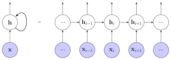
Figure 17. An example RNN network with hidden-to-hidden recurrent connections. The RNN has a repetitive structure. The left hand side, the recurrent graph is shown, while it is unfolded on the right. At every step $i$, the embedding $\bm{x}_{i}$ of a token in the sequence is fed into the RNN.

Recurrent Neural Networks (RNN) can process varying length input sequences such as characters or word tokens in a SQL query. Figure 17 shows a standard RNN network. Standard RNNs suffer from the vanishing gradient problem. In particular, during training, the gradient vector can grow or decay exponentially (Tai et al., 2015; Goodfellow et al., 2016). LSTMs are a more effective variant of RNNs. They are equipped with a memory cell, which helps preserve the long-term dependencies better than standard RNNs. We describe the LSTM version from (Zaremba and Sutskever, 2014). The mathematical formulation for the LSTM is as follows:

$$\bm{\tilde{c}}_{i} =\tanh(\bm{W}_{c}\bm{x}_{i}+\bm{U}_{c}\bm{h}_{i-1}+\bm{b}_{c})$$

$$\bm{\Gamma}_{u} =\sigma(\bm{W}_{u}\bm{x}_{i}+\bm{U}_{u}\bm{h}_{i-1}+\bm{b}_{u})$$

$$\bm{\Gamma}_{f} =\sigma(\bm{W}_{f}\bm{x}_{i}+\bm{U}_{f}\bm{h}_{i-1}+\bm{b}_{f})$$

$$\bm{\Gamma}_{o} =\sigma(\bm{W}_{o}\bm{x}_{i}+\bm{U}_{o}\bm{h}_{i-1}+\bm{b}_{o})$$

$$\bm{c}_{i} =\bm{\Gamma}_{u}\odot\bm{\tilde{c}}_{i}+\bm{\Gamma}_{f}\odot\bm{c}_{i-1}$$

$$\bm{h}_{i} =\bm{\Gamma}_{o}\odot\tanh(\bm{c}_{i})$$

where $\odot$ is element-wise multiplication. The LSTM parameters are $\bm{W}_{c}$, $\bm{W}_{u}$, $\bm{W}_{f}$, $\bm{W}_{o},\bm{U}_{c}$, $\bm{U}_{u}$, $\bm{U}_{f}$, $\bm{U}_{o}$ that are weight matrices, and $\bm{b}_{c}$, $\bm{b}_{u}$, $\bm{b}_{f}$, $\bm{b}_{o}$ that are biases. The memory cell $\bm{c}_{i}\in\mathbb{R}^{k}$ helps model the long-term dependencies. The gates $\bm{\Gamma}_{i},\bm{\Gamma}_{f},\bm{\Gamma}_{o},\bm{\tilde{c}}_{i}\in\mathbb{R}^{k}$ help control the flow of information (Goodfellow et al., 2016). We use a three-layered LSTM model (shown in Figure 18).

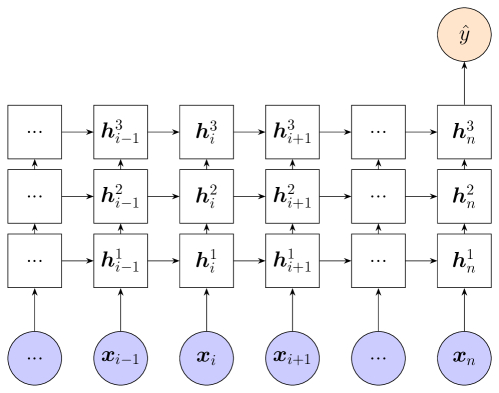
Figure 18. 3-layer LSTM model. Here $\bm{h}_{i}^{l}$ denotes the hidden state of an LSTM in layer $l$ at step $i$. At each step, $\bm{h}_{i}^{l}$ is fed as input to layer $l+1$. This allows the higher layers to capture more abstract concepts and longer term-dependencies.

A.3. Prediction and training

Having obtained a vector representation for each query, we need to learn the mapping from the vector to the query property, e.g.,  answer size. In the prediction stage, for the regression problems we pass this vector through a linear unit

$$\hat{y} =\bm{W}_{r}\bm{h}+\bm{b}_{r}$$

where $\bm{W}_{r}$ and $\bm{b}_{r}$ are the prediction model weight and bias parameters that should be learned. In classification problems, we pass $\bm{h}$ through a softmax layer, to produce the predicted target value

$$\hat{\bm{y}} =\textup{softmax}(\bm{W}_{s}\bm{h}+\bm{b}_{s})$$

where $\bm{W}_{s}$ and $\bm{b}_{s}$ are parameters that the model must learn. The softmax function is $\textup{softmax}(\bm{z})_{i}=\frac{\exp(z_{i})}{\sum_{j}^{n}\exp{z_{j}}}$.

Note, for three-layered LSTM $\bm{h}=\bm{h}_{n}^{3}$. For the CNN architecture, we also apply dropout and use $\bm{h}=(\bm{v}\circ\bm{g})$. Here, $\bm{v}\in\mathbb{R}^{K}$ is a masking vector of $K$ Bernoulli random variables with probability $p$ of being 1, and $\circ$ is element-wise multiplication. At train time, $\bm{v}$ randomly masks $\bm{g}$. Dropout helps prevent co-adaptation of the feature detectors (hinton2012improving).

Next, we discuss the objective functions we used to train the models and learn the parameters. In the regression problems, the goal to predict a real number for each query, which corresponds to either the answer size or CPU time. In Section 4.3.2 we observed the answer time and CPU time distributions had a large number of outliers. Therefore, for the regression problems we use the Huber loss function (Huber et al., 1964), that is a hybrid between $l_{2}$ for small residuals and $l_{1}$ for large residuals

(A.1) $$J(\theta) =\sum_{i=1}^{m}h(\hat{y}(\bm{x}_{i},\bm{\theta})-y_{i})$$

(A.2) $$h(r) =\begin{cases}0.5r^{2},&|r|\leq\epsilon\\ |r|-0.5,&|r|>\epsilon.\end{cases}$$

where $m$ is the number of instances (queries) in the train set, $\bm{\theta}$ is the set of all parameters that the model must learn, and $\hat{y}(\bm{x}_{i},\bm{\theta})$ is the predicted value, i.e., predicted CPU time for query $i$.

For error classification and session type classification, we use the cross entropy objective function

(A.3) $$J(\bm{\theta}) =\frac{1}{m}\sum_{i=1}^{m}-\log\hat{y}_{y_{i}}(\bm{x}_{i},\bm{\theta})$$

here $y_{i}$ is the label of the correct class for instance $i$, and $\hat{y}_{y_{i}}(\bm{x}_{i},\bm{\theta})$ is the probability of class $y_{i}$.

Note that while the traditional models fix the query vector representation (e.g., using the model explained in Section 5.1), and only optimize the weights of the prediction model, the neural network models jointly train the representation and the weights of the prediction model. This is captured in the set of parameters $\bm{\theta}$ that are learned for each model.

Appendix B SDSS Query Log Information

B.1. Query Session Class Assignment

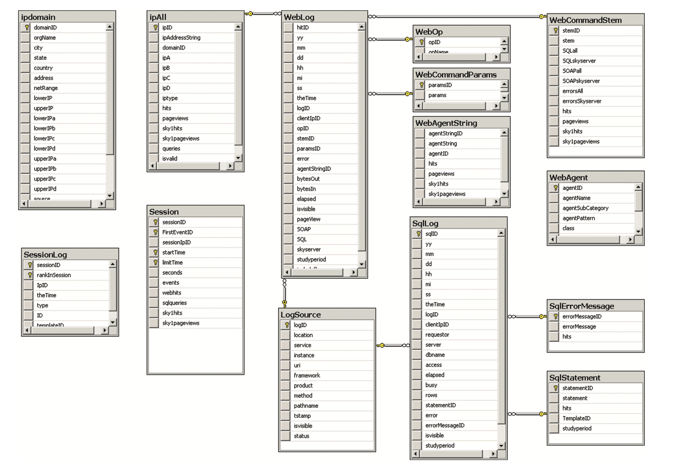
Figure 19. SDSS Query Logs Schema (from (Raddick et al., 2014a))

Name	Type	Description
yy	smallint	the year of the event
mm	tinyint	the month of the event
dd	tinyint	the day of the event
hh	tinyint	the hour of the event
mi	tinyint	the minute of the event
ss	tinyint	the second of the event
logID	int	the log that this came from, foreign key: LogSource.logID
seq	bigint	sequence number
clientIP	char(256)	the IP address of the client
op	char(8)	the operation (GET,POST,…)
command	varchar(7000)	the command executed
error	int	the error code if any
browser	varchar(2000)	the browser type
location	varchar(32)	the location of the site (FNAL, JHU,..
service	varchar(32)	type of service (SKYSERVER, SKYSERVICE, SKYQUERY,…)
instance	varchar(32)	The log underneath the service (V1, V2,.. )
uri	varchar(32)	The url or other ID for this service.
framework	varchar(32)	the calling framework (ASP,ASPX,HTML,QA,SOAP,…)
product	varchar(32)	the type of product acessed (EDR, DR1, DR2,…
PRIMARY KEY		(yy desc ,mm desc,dd desc,hh desc,mi desc,ss desc,seq desc,logID)

Table 8. WebLog Schema (from http://skyserver.sdss.org/log/en/traffic/sql.asp, Access date: May 2018.)

Name	Type	Description
theTime	datetime	the timestamp
webserver	varchar(64)	the url
winname	varchar(64)	the windows name of the server
clientIP	varchar(16)	client IP address
seq	int	sequence number to guarantee uniqueness of PK
server	varchar(32)	the name of the database server
dbname	varchar(32)	the name of the database
access	varchar(32)	The website DR1, collab,…
sql	varchar(7800)	the SQL statement
elapsed	real	the lapse time of the query
busy	real	the total CPU time of the query
rows	bigint	the number of rows generated
error	int	0 if ok, otherwise the sql error #; negative numbers are generated by the procedure
errorMessage	varchar(2000)	the error message.

Table 9. SqlLog Schema (from http://skyserver.sdss.org/log/en/traffic/sql.asp, Access date: May 2018.)

Figure 19 shows the SDSS schema from (Raddick et al., 2014a). Tables 8 and8 show a detailed description of the WebLog and SqlLog tables. Each session in SDSS can have a mix of SQL query entries and webhit entries. The SQL query entries are in the “SQLLog” table with a unique SQLLog.sqlID, while webhit entries are in the “WebLog” table with a unique WebLog.hitID. The “SqlLog” table contains around 194M entries which we refer to SQL query logs. The session information is in the “Session” table, which contains the number of SQL entries (Session.sqlqueries) and the number of webhits (Session.webhits). The “SessionLog” table contains more detailed information for the sessions. In particular, if SessionLog.type is 0, then SessionLog.ID is a foreign key pointing to WebLog.hitID. if SessionLog.type is 1, then SessionLog.ID is a foreign key pointing to SqlLog.sqlID.

Sessions with webhits have entries in the WebLog table, and include a WebLog.agentStringIDs. Based on (Singh et al., 2007), we submitted the following SQL query on CasJobs:

⬇

SELECT dbo.webAgentString.agentStringID, dbo.WebAgent.class into mydb.agentStringIDClass

FROM dbo.webAgentString, dbo.WebAgent

WHERE dbo.webAgentString.agentID = dbo.WebAgent.agentID

ORDER BY dbo.webAgentString.agentStringID

It retrieved a table “agentStringIDClass” with 578,627 entries. In this table, the WebAgent.class attribute has 6 unique values: UNKNOWN, BOT, ADMIN, PROGRAM, ANONYMOUS, BROWSER. Therefore, sessions with webhit entries are assigned at least one of these 6 values. To assign a “Session Class” to these sessions, and their corresponding SQL queries, we do a majority vote among the webhits of the session. However, even if one webhit entry with “BOT” exists for a session, then we assign the class “BOT” to the entire session, regardless of the outcome of the vote. For sessions that do not have have a webhit entry, an explicit class is not considered in the SDSS dataset. We assigned the “noWebhit” class for SQL queries that belong to these sessions.

B.2. Exception Handling

In our processing, we had to handle two exceptions:

• There were entries in SqlLog with errorMessageID that did not exist in corresponding SqlErrorMessage table. But SqlErrorMessage.errorMessageID is a primary key. Instead of eliminating these entries we handled this exception by creating a temporary entry for them in the final dataset output, with an appropriate description.

• Around 4870578 entries in SqlLog had SqlLog.statementID equal to zero. But SqlStatement.statementID is a primary key in the SqlStatment table, and does not have a zero value. We eliminated these SqlLog entries in our full dataset. So the difference of 194113641 - 4870578 = 189243063 is due to this step. Therefore, although SqlLog had 194113641 entries, our final full dataset has 189243063 entries.

Another problem, is that several entries in SqlStatement had an empty statement but had different statementIDs and TemplateIDs. We handle this problem when we sample from the full data. Specifically, for these SqlLog entries we modify the statement to ’Empty’ string.

B.3. Repetition of Query Statements

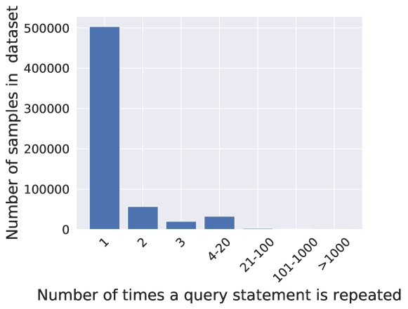
Figure 20. Histogram of the number of times a query statement is repeated in a dataset consisting of randomly sampled queries from each session.

We found that some SQL query logs have the same query statement, albeit varying values for properties such as session class, error class, answer size, and CPU time. This is because the same query statement may be submitted in different sessions, via different access interfaces, and against different versions of the database.

To collect a dataset we proceed as follows: First, we randomly sampled a SQL query log from each session in the pre-processed query workload. This resulted in a total of 1,563,386 SQL query logs. Next, we grouped SQL query logs with the same query statement. This results in 618,053 groups or unique statements. We found approximately 81.5% of these unique statements only appear in one SQL query log. Figure 20 shows the histogram of the number of times a query statement is repeated in the dataset. For the remaining 18.5% of the query statements, we aggregated their meta-data labels. In particular, for answer size, and CPU time we use the average of value as the label of the statement. For session class, and error class, we considered the majority class and used it as the label of the statement. Our final dataset consists of 618,053 statements and corresponding meta-data.

References

- (1)
- t-r ([n. d.]) [n. d.]. http://www.cs.ubc.ca/~zolaktaf.
- Akdere et al. (2012) Mert Akdere, Ugur Çetintemel, Matteo Riondato, Eli Upfal, and Stanley B Zdonik. 2012. Learning-Based Query Performance Modeling and Prediction. In ICDE. 390–401.
- Allamanis et al. (2018) Miltiadis Allamanis, Earl T Barr, Premkumar Devanbu, and Charles Sutton. 2018. A Survey of Machine Learning for Big Code and Naturalness. Comput. Surveys 51, 4 (2018), 81.
- Bai et al. (2018) Shaojie Bai, J. Zico Kolter, and Vladlen Koltun. 2018. An Empirical Evaluation of Generic Convolutional and Recurrent Networks for Sequence Modeling. ArXiv 1803.01271 (2018).
- Bengio (2011) Yoshua Bengio. 2011. Deep Learning of Representations for Unsupervised and Transfer Learning. In UTLW. 17–37.
- Bergamaschi et al. (2011) Sonia Bergamaschi, Elton Domnori, Francesco Guerra, Raquel Trillo Lado, and Yannis Velegrakis. 2011. Keyword Search over Relational Databases: A Metadata Approach. In SIGMOD. 565–576.
- Chatzopoulou et al. (2009) Gloria Chatzopoulou, Magdalini Eirinaki, and Neoklis Polyzotis. 2009. Query Recommendations for Interactive Database Exploration. In SSDBM. 3–18.
- Chaudhuri et al. (2002) Surajit Chaudhuri, Ashish Kumar Gupta, and Vivek Narasayya. 2002. Compressing SQL Workloads. In SIGMOD. 488–499.
- Conneau et al. (2016) Alexis Conneau, Holger Schwenk, Loïc Barrault, and Yann Lecun. 2016. Very Deep Convolutional Networks for Text Classification. ArXiv 1606.01781 (2016).
- Dimitriadou et al. (2014) Kyriaki Dimitriadou, Olga Papaemmanouil, and Yanlei Diao. 2014. Explore-by-Example: An Automatic Query Steering Framework for Interactive Data Exploration. In SIGMOD. 517–528.
- Ding et al. (2019) Bailu Ding, Sudipto Das, Ryan Marcus, Wentao Wu, Surajit Chaudhuri, and Vivek Narasayya. 2019. AI Meets AI: Leveraging Query Executions to Improve Index Recommendations. In SIGMOD. 1241–1258.
- Eirinaki et al. (2014) Magdalini Eirinaki, Suju Abraham, Neoklis Polyzotis, and Naushin Shaikh. 2014. QueRIE: Collaborative Database Exploration. TKDE 26, 7 (2014), 1778–1790.
- Fan et al. (2011) Ju Fan, Guoliang Li, and Lizhu Zhou. 2011. Interactive SQL Query Suggestion: Making Databases User-Friendly. In ICDE. 351–362.
- Ganapathi et al. (2009) Archana Ganapathi, Harumi Kuno, Umeshwar Dayal, Janet L Wiener, Armando Fox, Michael Jordan, and David Patterson. 2009. Predicting Multiple Metrics for Queries: Better Decisions Enabled by Machine Learning. In ICDE. 592–603.
- Goodfellow et al. (2016) Ian Goodfellow, Yoshua Bengio, and Aaron Courville. 2016. Deep Learning. MIT Press.
- Google (2010) Google. 2010. Big Query. https://cloud.google.com/bigquery/.
- Hacigümüş et al. (2002) Hakan Hacigümüş, Bala Iyer, Chen Li, and Sharad Mehrotra. 2002. Executing SQL over Encrypted Data in the Database-Service-Provider Model. In SIGMOD. 216–227.
- Huber et al. (1964) Peter J Huber et al. 1964. Robust estimation of a location parameter. The Annals of Mathematical Statistics 35, 1 (1964), 73–101.
- Inc. (2012a) Amazon Inc. 2012a. Amazon Redshift. https://aws.amazon.com/redshift/.
- Inc. (2012b) Snowflake Inc. 2012b. Snowflake. https://www.snowflake.com/.
- Jagadish et al. (2007) HV Jagadish, Adriane Chapman, Aaron Elkiss, Magesh Jayapandian, Yunyao Li, Arnab Nandi, and Cong Yu. 2007. Making Database Systems Usable. In SIGMOD. 13–24.
- Jain and Howe (2018) Shrainik Jain and Bill Howe. 2018. Query2Vec: NLP Meets Databases for Generalized Workload Analytics. ArXiv 1801.05613 (2018).
- Jain et al. (2016) Shrainik Jain, Dominik Moritz, Daniel Halperin, Bill Howe, and Ed Lazowska. 2016. SQLShare: Results from a Multi-Year SQL-as-a-Service Experiment. In SIGMOD. 281–293.
- Jain et al. (2018) Shrainik Jain, Jiaqi Yan, Thierry Cruane, and Bill Howe. 2018. Database-Agnostic Workload Management. ArXiv 1808.08355 (2018).
- Jayapandian and Jagadish (2009) Magesh Jayapandian and HV Jagadish. 2009. Automating the Design and Construction of Query Forms. TKDE 21, 10 (2009), 1389–1402.
- Johnson and Zhang (2014) Rie Johnson and Tong Zhang. 2014. Effective Use of Word Order for Text Categorization with Convolutional Neural Networks. ArXiv 1412.1058 (2014).
- Johnson and Zhang (2015) Rie Johnson and Tong Zhang. 2015. Semi-Supervised Convolutional Neural Networks for Text Categorization via Region Embedding. In Advances in Neural Information Processing Systems. 919–927.
- Johnson and Zhang (2016a) Rie Johnson and Tong Zhang. 2016a. Convolutional neural networks for text categorization: Shallow Word-Level vs. Deep Character-Level. ArXiv 1609.00718 (2016).
- Johnson and Zhang (2016b) Rie Johnson and Tong Zhang. 2016b. Supervised and Semi-Supervised Text Categorization using LSTM for Region Embeddings. In ICML. 526–534.
- Johnson and Zhang (2017) Rie Johnson and Tong Zhang. 2017. Deep Pyramid Convolutional Neural Networks for Text Categorization. In ACL. 562–570.
- Khoussainova et al. (2010) Nodira Khoussainova, YongChul Kwon, Magdalena Balazinska, and Dan Suciu. 2010. SnipSuggest: Context-Aware Autocompletion for SQL. PVLDB 4, 1 (2010), 22–33.
- Kim (2014) Yoon Kim. 2014. Convolutional Neural Networks for Sentence Classification. ArXiv 1408.5882 (2014).
- Kim et al. (2016) Yoon Kim, Yacine Jernite, David Sontag, and Alexander M Rush. 2016. Character-Aware Neural Language Models.. In AAAI. 2741–2749.
- Kingma and Ba (2014) Diederik P Kingma and Jimmy Ba. 2014. Adam: A Method for Stochastic Optimization. ArXiv 1412.6980 (2014).
- Kul et al. (2016) Gokhan Kul, Duc Luong, Ting Xie, Patrick Coonan, Varun Chandola, Oliver Kennedy, and Shambhu Upadhyaya. 2016. Ettu: Analyzing Query Intents in Corporate Databases. In WWW. 463–466.
- LeCun et al. (1989) Yann LeCun, Bernhard Boser, John S Denker, Donnie Henderson, Richard E Howard, Wayne Hubbard, and Lawrence D Jackel. 1989. Backpropagation Applied to Handwritten Zip Code Recognition. Neural computation 1, 4 (1989), 541–551.
- Leis et al. (2015) Viktor Leis, Andrey Gubichev, Atanas Mirchev, Peter Boncz, Alfons Kemper, and Thomas Neumann. 2015. How Good Are Query Optimizers, Really? PVLDB 9, 3 (2015), 204–215.
- Li and Jagadish (2014) Fei Li and HV Jagadish. 2014. Constructing an Interactive Natural Language Interface for Relational Databases. PVLDB 8, 1 (2014), 73–84.
- Li et al. (2012) Jiexing Li, Arnd Christian König, Vivek Narasayya, and Surajit Chaudhuri. 2012. Robust Estimation of Resource Consumption for SQL Queries using Statistical Techniques. PVLDB 5, 11 (2012), 1555–1566.
- Liu et al. (2015) Henry Liu, Mingbin Xu, Ziting Yu, Vincent Corvinelli, and Calisto Zuzarte. 2015. Cardinality Estimation using Neural Networks. In CASCON. 53–59.
- Nguyen et al. (2015) Hoang Vu Nguyen, Klemens Böhm, Florian Becker, Bertrand Goldman, Georg Hinkel, and Emmanuel Müller. 2015. Identifying User Interests within the Data Space-a Case Study with SkyServer.. In EDBT. 641–652.
- O’Mullane et al. (2005) William O’Mullane, Nolan Li, María Nieto-Santisteban, Alex Szalay, Ani Thakar, and Jim Gray. 2005. Batch is Back: CasJobs, Serving Multi-TB Data on the Web. In ICWS. 33–40.
- Parr (2013) Terence Parr. 2013. The Definitive ANTLR 4 Reference. Pragmatic Bookshelf.
- Pedregosa et al. (2011) F. Pedregosa, G. Varoquaux, A. Gramfort, V. Michel, B. Thirion, O. Grisel, M. Blondel, P. Prettenhofer, R. Weiss, V. Dubourg, J. Vanderplas, A. Passos, D. Cournapeau, M. Brucher, M. Perrot, and E. Duchesnay. 2011. Scikit-Learn: Machine Learning in Python. JMLR 12 (2011), 2825–2830.
- Raddick et al. (2014a) M Jordan Raddick, Ani R Thakar, Alexander S Szalay, and Rafael DC Santos. 2014a. Ten Years of SkyServer I: Tracking Web and SQL e-Science Usage. Computing in Science & Engineering 16, 4 (2014), 22–31.
- Raddick et al. (2014b) M Jordan Raddick, Ani R Thakar, Alexander S Szalay, and Rafael DC Santos. 2014b. Ten Years of SkyServer II: How Astronomers and the Public Have Embraced e-Science. Computing in Science & Engineering 16, 4 (2014), 32–40.
- Shen et al. (2014) Yanyan Shen, Kaushik Chakrabarti, Surajit Chaudhuri, Bolin Ding, and Lev Novik. 2014. Discovering Queries Based on Example Tuples. In SIGMOD. 493–504.
- Singh et al. (2007) Vik Singh, Jim Gray, Ani Thakar, Alexander S Szalay, Jordan Raddick, Bill Boroski, Svetlana Lebedeva, and Brian Yanny. 2007. Skyserver Traffic Report - The First Five Years. ArXiv 0701173 (2007).
- Stefanidis et al. (2009) Kostas Stefanidis, Marina Drosou, and Evaggelia Pitoura. 2009. “You May Also Like” Results in Relational Databases. In PersDB. 37–42.
- Szalay (2018) Alexander S Szalay. 2018. From SkyServer to SciServer. AAPSS 675, 1 (2018), 202–220.
- Szalay et al. (2002) Alexander S Szalay, Jim Gray, Ani R Thakar, Peter Z Kunszt, Tanu Malik, Jordan Raddick, Christopher Stoughton, and Jan vandenBerg. 2002. The SDSS Skyserver: Public Access to the Sloan Digital Sky Server Data. In SIGMOD. 570–581.
- Tai et al. (2015) Kai Sheng Tai, Richard Socher, and Christopher D Manning. 2015. Improved Semantic Representations From Tree-Structured Long Short-Term Memory Networks. ArXiv 1503.00075 (2015).
- TPC (2018) TPC. 2018. TPC Benchmarks. http://www.tpc.org.
- Wang et al. (2016) Wei Wang, Meihui Zhang, Gang Chen, H. V. Jagadish, Beng Chin Ooi, and Kian-Lee Tan. 2016. Database Meets Deep Learning: Challenges and Opportunities. SIGMOD Rec. 45, 2 (2016), 17–22.
- Yin et al. (2017) Wenpeng Yin, Katharina Kann, Mo Yu, and Hinrich Schütze. 2017. Comparative Study of CNN and RNN for Natural Language Processing. ArXiv 1702.01923 (2017).
- Yosinski et al. (2014) Jason Yosinski, Jeff Clune, Yoshua Bengio, and Hod Lipson. 2014. How Transferable Are Features in Deep Neural Networks?. In NIPS. 3320–3328.
- Young et al. (2018) Tom Young, Devamanyu Hazarika, Soujanya Poria, and Erik Cambria. 2018. Recent Trends in Deep Learning Based Natural Language Processing. IEEE Computational Intelligence Magazine 13, 3 (2018), 55–75.
- Zaremba and Sutskever (2014) Wojciech Zaremba and Ilya Sutskever. 2014. Learning to Execute. ArXiv 1410.4615 (2014).
- Zeng et al. (2014) Zhong Zeng, Zhifeng Bao, Thuy Ngoc Le, Mong Li Lee, and Wang Tok Ling. 2014. ExpressQ: Identifying Keyword Context and Search Target in Relational Keyword Queries. In CIKM. 31–40.
- Zhang et al. (2015) Xiang Zhang, Junbo Zhao, and Yann LeCun. 2015. Character-Level Convolutional Networks for Text Classification. In NIPS. 649–657.
- Zhong et al. (2017) Victor Zhong, Caiming Xiong, and Richard Socher. 2017. Seq2SQL: Generating Structured Queries From Natural Language using Reinforcement Learning. ArXiv 1709.00103 (2017).