Orbits of Bernoulli Measures in Cellular Automata

Glossary

Configuration space

Set of all bisequences of symbols from the alphabet $\mathcal{A}$ of $N$ symbols, $\mathcal{A}=\{0,1,\ldots,N-1\}$, denoted by $\mathcal{A}^{\mathbbm{Z}}$. Elements of $\mathcal{A}^{\mathbbm{Z}}$ are called configurations and denoted by bold lowercase letters: $\mathbf{x}$, $\mathbf{y}$, etc.

Block or word

A finite sequence of symbols of the alphabet $\mathcal{A}$. Set of all blocks of length $n$ is denoted by $\mathcal{A}^{n}$, while the sent of all possible blocks of all lengths by $\mathcal{A}^{\star}$. Blocks are denoted by bold lowercase letters $\mathbf{a}$, $\mathbf{b}$, $\mathbf{c}$, etc. Individual symbols of the block $\mathbf{b}$ are denoted by indexed italic form of the same letter, $\mathbf{b}=b_{1},b_{2},\ldots,b_{n}$. To make formulae more compact, commas are sometimes dropped (if no confusion arises), and we simply write $\mathbf{b}=b_{1}b_{2}\ldots b_{n}$.

Cylinder set

For a block $\mathbf{b}$ of length $n$, the cylinder set generated by $\mathbf{b}$ and anchored at $i$ is the subset of configurations such that symbols at positions from $i$ to $i+n-1$ are fixed and equal to symbols in the block $\mathbf{b}$, while the remaining symbols are arbitrary. Denoted by $[\mathbf{b}]_{i}=\{\mathbf{x}\in{\mathcal{A}}^{\mathbb{Z}}:\mathbf{x}_{[i,i+n)}=\mathbf{b}\}$.

Cellular automaton

In this article, cellular automaton is understood as a map $F$ in the space of shift-invariant probability measures over the configuration space $\mathcal{A}^{\mathbbm{Z}}$. To define $F$, two ingredients are needed, a positive integer $r$ called radius and a function $w:\mathcal{A}\times\mathcal{A}^{2r+1}\to[0,1]$, whose values are called transition probabilities. The image of a measure $\mu$ under the action of $F$ is then defined by probabilities of cylinder sets, $(F\mu)([\mathbf{a}]_{i})=\sum_{\mathbf{b}\in\mathcal{A}^{|\mathbf{a}|+2r}}w(\mathbf{a}|\mathbf{b})\mu([\mathbf{b}]_{i-r})$ where $i\in\mathbb{Z}$, $\mathbf{a}\in\mathcal{A}^{\star}$, and where $w(\mathbf{a}|\mathbf{b})$ is defined as $w(\mathbf{a}|\mathbf{b})=\prod_{j=1}^{|\mathbf{a}|}w(a_{j}|b_{j}b_{j+1}\ldots b_{j+2r})$. Cellular automaton is called deterministic if transition probabilities take values exclusively in the set $\{0,1\}$, otherwise it is called probabilistic.

Orbit of a measure

For a given cellular automaton $F$ and a given shift invariant probability measure $\mu$, the orbit of $\mu$ under $F$ is a sequence $\mu,F\mu,F^{2}\mu,F^{3}\mu,\ldots$. The main subject of this article are orbits of Bernoulli measures on $\{0,1\}^{\mathbbm{Z}}$, that is, measures parametrized by $p\in[0,1]$ and defined by $\mu_{p}([\mathbf{b}])=p^{\#_{1}(\mathbf{b})}(1-p)^{\#_{0}(\mathbf{b})}$, where $\#_{k}(\mathbf{b})$ denotes number of symbols $k$ in $\mathbf{b}$.

Block probability

Probability of occurence of a given block $\mathbf{b}$ (or word) of symbols. Formally defined as a measure of the cylinder set generated by the block $\mathbf{b}$ and anchored at $i$, and denoted by $P(\mathbf{b})=\mu([\mathbf{b}]_{i})$. In this article we are exclusively dealing with shift-invariant probability measures, thus $\mu([\mathbf{b}]_{i})$ is independent of $i$. Probability of occurence of a block $\mathbf{b}$ after $n$ iterations of cellular automaton $F$ starting from initial measure $\mu$ is denoted by $P_{n}(\mathbf{b})$ and defined as $P_{n}(\mathbf{b})=(F^{n}\mu)([\mathbf{b}]_{i})$. Here again we assume shift invariance, thus $(F^{n}\mu)([\mathbf{b}]_{i})$ is independent of $i$.

Short/long block representation

Shift invariant probability measures on $\mathcal{A}^{\mathbbm{Z}}$ are unambiguously determined by block probabilities $P(\mathbf{b})$, $\mathbf{b}\in\mathcal{A}^{\star}$. For a given $k$, probabilities of blocks of length $1,2,\ldots,k$ are not all independent, as they have to satisfy measure additivity conditions, known as Kolmogorov consistency conditions. One can show that only $(N-1)N^{k-1}$ of them are linearly independent. If one declares as independent the set of $(N-1)N^{k-1}$ blocks chosen so that they are as short blocks as possible, one can express the remaining blocks probabilities in terms of these. An algorithm for selection of shortest possible blocks is called short block representation. If, on the other hand, one chooses the longest possible blocks to be declared independent, this is called long block representation.

Local structure approximation

Approximation of points of the orbit of a measure $\mu$ under a given cellular automaton $F$ by Markov measures, that is, measures maximizing entropy and completely determined by probabilities of blocks of length $k$. The number $k$ is called the order or level of local structure approximation.

Block evolution operator

When the cellular automaton rule of radius $r$ is deterministic, its transition probabilities take values in the set $\{0,1\}$. For such rules and for $\mathcal{A}=\{0,1\}$, define the local function $f:\mathcal{A}^{2r+1}\to\mathcal{A}$ by $f(x_{1},x_{2},\ldots x_{2r+1})$ $=w(1|x_{1},x_{2},\ldots x_{2r+1})$ for all $x_{1},x_{2},\ldots x_{2r+1}\in\mathcal{A}$. A block evolution operator corresponding to $f$ is a mapping ${\mathbf{f}}:\mathcal{A}^{\star}\mapsto\mathcal{A}^{\star}$ defined for $a=a_{0}a_{1}\ldots a_{n-1}\in\mathcal{A}^{n}$ by $f(a)=\{f(a_{i},a_{i+1},\ldots,a_{i+2r})\}_{i=0}^{n-2r-1}$. For a deterministic cellular automaton $F$ its local function is denoted by the corresponding lowercase italic form of the same letter, $f$, while the block evolution operator is the bold form of the same letter, $\mathbf{f}$. The set of preimages of the block $\mathbf{a}$ under ${\mathbf{f}}$ is called block preimage set, denoted by ${\mathbf{f}}^{-1}(\mathbf{a})$.

Complete set set

A set of words $C=\{\mathbf{a}_{1},\mathbf{a}_{2},\mathbf{a}_{3},\ldots\}$ is called complete with respect to a CA rule $F$ if for every $\mathbf{a}\in C$ and $n\in\mathbb{N}$, $P_{n+1}(\mathbf{a})$ can be expressed as a linear combination of $P_{n}(\mathbf{a}_{1}),P_{n}(\mathbf{a}_{2}),P_{n}(\mathbf{a}_{3}),\ldots$.

Contents

1. 1 Introduction
2. 2 Construction of a probability measure
3. 3 Description of probability measures by block probabilities
4. 4 Cellular automata
5. 5 Bayesian approximation
6. 6 Local structure maps
7. 7 Exact calculations of probabilities of short blocks along the orbit
   1. 7.1 Balanced preimages: surjective rules
   2. 7.2 Preimages with long runs and arbitrary symbols: rule 130
   3. 7.3 Preimages described by a local property: rule 172
   4. 7.4 Preimages described by a non-local property: rule 184
   5. 7.5 Preimage sets related to preimages of other solvable rules: rule 14
   6. 7.6 Convergence of block probabilities
8. 8 Examples of exact results for probabilistic CA rules
   1. 8.1 Rule 200A
   2. 8.2 Rule 140A
   3. 8.3 Complete sets
9. 9 Future directions

1 Introduction

In both theory and applications of cellular automata (CA), one of the most natural and most frequently encountered problems is what one could call the density response problem: If the proportion of ones (or other symbols) in the initial configuration drawn from a Bernoulli distribution is known, what is the expected proportion of ones (or other symbols) after $n$ iterations of the CA rule? One could rephrase it in a slightly different form: if the probability of occurence of a given symbol in an initial configuration is known, what is the probability of occurrence of this symbol after $n$ iterations of this rule?

A similar question could be asked about the probability of occurence of longer blocks of symbols after $n$ iterations of the rule. Due to complexity of CA dynamics, there is no hope to answer questions like this in a general form, for an arbitrary rule. The situation is somewhat similar to hat we encounter in the theory of differential equations: there is no general algorithm for solving initial value problem for an arbitrary rule, but one can either solve it approximately (by numerical method), or, for some differential equations, one can construct the solution formula in terms of elementary functions.

In cellular automata, there are also two ways to make progress. One is to use some approximation techniques, and compute approximate values of the desired probabilities. Another is to focus on narrower classes of CA rules, with sufficiently simple dynamics, and attempt to compute these probabilities in a rigorous ways. Both these approaches are discussed in this article.

We will treat cellular automata as maps in the space of Borel shift-invariant probability measures, equipped with the so-called weak$\star$ topology (Kůrka and Maass, 2000; Kůrka, 2005; Pivato, 2009; Formenti and Kůrka, 2009). In this setting, the aforementioned problem of computing block probabilities can be posed as the problem of determining the orbit of given initial measure $\mu$ (usually a Bernoulli measure) under the action of a given cellular automaton. Since computing the complete orbit of a measure is, in general, very difficult, approximate methods have been developed. The simplest of these methods is called the mean-field theory, and has its origins in statistical physics (Wolfram, 1983). The main idea behind the mean-field theory is to approximate the consecutive iterations of the initial measure by Bernoulli measures, ignoring correlations between sites. While this approximation is obviously very crude, it is sometimes quite useful in applications.

In 1987, H. A. Gutowitz, J. D. Victor, and B. W. Knight proposed a generalization of the mean-field theory for cellular automata which, unlike the mean-field theory, takes into account correlations between sites, although only in an approximate way (Gutowitz et al, 1987). The basic idea is to approximate the consecutive iterations of the initial measure by Markov measures, also called finite block measures. Finite block measures of order $k$ are completely determined by probabilities of blocks of length $k$. For this reason, one can construct a map on these block probabilities, which, when iterated, approximates probabilities of occurrence of the same blocks in the actual orbit of a given cellular automaton. The construction of Markov measures is based on the idea of “Bayesian extension”, introduced in 1970s and 80s in the context of lattice gases (Brascamp, 1971; Fannes and Verbeure, 1984). The local structure theory produces remarkably good approximations of probabilities of small blocks, provided that one uses sufficiently high order of the Markov measure.

For deterministic CA, if one wants to compute probabilities of small block exactly, without using any approximations, one has to study combinatorial structure of preimages of these block under the action of the rule. In many cases, this reveals some regularities which can be exploited in computation of block probabilities. For a number of elementary CA rules, this approach has been used to construct probabilities of short blocks, typically block of up to three symbols. For probabilistic cellular automata, one can try to compute $n$-step transition probabilities, and in some cases these transition probabilities are expressible in terms of elementary functions. This allows to construct formulae for block probabilities.

In the rest of this article we will discuss how to construct shift-invariant probability measures over the space of bisequences of symbols, and how to describe such measures in terms of block probabilities. We will then define cellular automata as maps in the space of measures and discuss orbits of shift-invariant probability measures under these maps. Subsequently, the local structure approximation will be discussed as a method to approximate orbits of Bernoulli measures under the action of cellular automata. The final sections presents some known examples of cellular automata, both deterministic and probabilistic, for which elements of the orbit of the Bernoulli measure (probabilities of short blocks) can be determined exactly.

2 Construction of a probability measure

Let ${\mathcal{A}}=\{0,1,\ldots,N-1\}$ be called an alphabet, or a symbol set, and let $X={\mathcal{A}}^{\mathbb{Z}}$ be called the configurations space. The Cantor metric on $X$ is defined as $d(\mathbf{x},\mathbf{y})=2^{-k}$, where $k=\mathrm{min}\{|i|:\mathbf{x}_{i}\neq\mathbf{y}_{i}\}$. $X$ with the metric $d$ is a Cantor space, that is, compact, totally disconnected and perfect metric space. A finite sequence of elements of ${\mathcal{A}}$, $\mathbf{b}=b_{1}b_{2}\ldots,b_{n}$ will be called a block (or word) of length $n$. Set of all blocks of elements of ${\mathcal{A}}$ of all possible lengths will be denoted by ${\mathcal{A}}^{\star}$. A cylinder set generated by the block $\mathbf{b}=b_{1}b_{2}\ldots,b_{n}$ and anchored at $i$ is defined as

$$[\mathbf{b}]_{i}=\{\mathbf{x}\in{\mathcal{A}}^{\mathbb{Z}}:\mathbf{x}_{[i,i+n)}=\mathbf{b}\}.$$ (1)

When one of the indices $i,i+1,\ldots,i+n-1$ is equal to zero, the cylinder set will be called elementary. The collection (class) of all elementary cylinder sets of $X$ together with the empty set and the whole space $X$ will be denoted by $\mathit{Cyl}(X)$. One can show that $\mathit{Cyl}(X)$ constitutes a semi-algebra over $X$. Moreover, one can show that any finitely additive map $\mu:\mathit{Cyl}(X)\to[0,\infty]$ for which $\mu(\varnothing)=0$ is a measure on the semi-algebra of elementary cylinder sets $\mathit{Cyl}(X)$.

The semi-algebra of elementary cylinder sets, equipped with a measure is still “too small” a class of subsets of $X$ to support all requirements of probability theory. For this we need a $\sigma$-algebra, that is, a class of subsets of $X$ that is closed under the complement and under the countable unions of its members. Such $\sigma$-algebra can be defined as an “extension” of $\mathit{Cyl}(X)$. The smallest $\sigma$-algebra containing $\mathit{Cyl}(X)$ will be called $\sigma$-algebra generated by $\mathit{Cyl}(X)$. As it turns out, it is possible to extend a measure on semi-algebra to the $\sigma$-algebra generated by it, by using Hahn-Kolmogorov theorem.

In what follows, we will only consider measures for which $\mu(X)=1$ (probability measures). Moreover, we will only limit our attention to the case of translationally invariant measures (also called shift-invariant), by requiring that, for all $\mathbf{b}\in{\mathcal{A}}^{\star}$, $\mu([\mathbf{b}]_{i})$ is independent of $i$. To simplify notation, we then define $P:{\mathcal{A}}^{\star}\to[0,1]$ as

$$P(\mathbf{b}):=\mu([\mathbf{b}]_{i}).$$ (2)

Values $P(\mathbf{b})$ will be called block probabilities. Application of Hahn-Kolmogorov theorem to the case of shift-invariant probability measure $\mu$ yields the following result.

Theorem 1

Let $P:{\mathcal{A}}^{\star}\to[0,1]$ satisfy the conditions

$$P(\mathbf{b}) =\sum_{a\in{\mathcal{A}}}P(\mathbf{b}a)=\sum_{a\in\cal{G}}P(a\mathbf{b})\,\,\,\,\,\,\,\forall{\mathbf{b}\in{\mathcal{A}}^{\star}},$$ (3)

$$1 =\sum_{a\in\cal{A}}P(a).$$ (4)

Then $P$ uniquely determines shift-invariant probability measure on the $\sigma$-algebra generated by elementary cylinder sets of $X$.

The set of shift-invariant probability measures on the $\sigma$-algebra generated by elementary cylinder sets of $X$ will be denoted by $\mathfrak{M}(X)$.

Conditions (3) and (4) are often called consistency conditions, although they are essentially equivalent to measure additivity conditions. Some consequences of consistency conditions in the context of cellular automata have been studied in detail by McIntosh (2009).

3 Description of probability measures by block probabilities

Since the probabilities $P(\mathbf{b})$ uniquely determine the probability measure, we can define a shift-invariant probability measure by specifying $P(\mathbf{b})$ for all $\mathbf{b}\in\mathcal{A}^{\star}$. Obviously, because of consistency conditions, block probabilities are not independent, thus in order to define the probability measure, we actually need to specify only some of them, but not necessarily all - the missing ones can be computed by using consistency conditions.

Define $\mathbf{P}^{(k)}$ to be the column vector of all probabilities of blocks of length $k$ arranged in lexical order. For example, for ${\mathcal{A}}=\{0,1\}$, these are

$$\mathbf{P}^{(1)} =[P(0),P(1)]^{T},$$

$$\mathbf{P}^{(2)} =[P(00),P(01),P(10),P(11)]^{T},$$

$$\mathbf{P}^{(3)} =[P(000),P(001),P(010),P(011),P(100),P(101),P(110),P(111)]^{T},$$

$$\cdots.$$

The following result (Fukś, 2013) is a direct consequence of consistency conditions of eq. (3) and (4).

Proposition 1

Among all block probabilities constituting components of $\mathbf{P}^{(1)}$, $\mathbf{P}^{(2)}$, $\dots,\mathbf{P}^{(k)}$ only $(N-1)N^{k-1}$ are linearly independent.

For example, for $N=2$ and $k=3$, among $\mathbf{P}^{(1)},\mathbf{P}^{(2)},\mathbf{P}^{(3)}$ (which have, in total, $8+4+2=14$ components), there are only 4 independent blocks. These four block can be selected somewhat arbitrarily (but not completely arbitrarily). Two methods or algorithms for selection of independent blocks are especially convenient.

The first one is called long block representation. It is based on the following property (cf. ibid.).

Proposition 2

Let $\mathbf{P}^{(k)}$ be partitioned into two sub-vectors, $\mathbf{P}^{(k)}=(\mathbf{P}^{(k)}_{Top}$, $\mathbf{P}^{(k)}_{Bot})$, where $\mathbf{P}^{(k)}_{Top}$ contains first $N^{k}-N^{k-1}$ entries of $\mathbf{P}^{(k)}$, and $\mathbf{P}^{(k)}_{Bot}$ the remaining $N^{k-1}$ entries. Then

$$\mathbf{P}^{(k)}_{Bot}=\left[\begin{array}[]{c}0\\ \vdots\\ 0\\ 1\end{array}\right]-\left(\mathbf{B}^{(k)}\right)^{-1}\mathbf{A}^{(k)}\mathbf{P}^{(k)}_{Top}.$$ (5)

In the above, matrix $\mathbf{B}^{(k)}$ is constructed from zero $N^{k-1}\times N^{k-1}$ matrix by placing $-1$’s on the diagonal, and then filling the last row with 1’s, so that

$$\mathbf{B}^{(k)}=\left[\begin{array}[]{rrrr}-1&0&\cdots&0\\ 0&-1&&\\ \vdots&&\ddots&\\ 1&1&1&1\end{array}\right].$$ (6)

The matrix $\mathbf{A}^{(k)}$ is a bit more complicated,

$$\mathbf{A}^{(k)}=[\mathbf{J}_{1}\mathbf{J}_{2}\ldots\mathbf{J}_{N-1}]+[\,\underbrace{\mathbf{B}^{(k)}\,\,\,\mathbf{B}^{(k)}\ldots\mathbf{B}^{(k)}}_{N-1}\,],$$ (7)

where $\mathbf{J}_{m}$ is an $N^{k-1}\times N^{k-1}$ matrix in which $m$-th row consist of all 1’s, and all other entries are equal to 0.

The above proposition means that among block probabilities constituting components of $\mathbf{P}^{(1)}$ , $\mathbf{P}^{(2)},\dots,\mathbf{P}^{(k)}$, we can treat first $N^{k}-N^{k-1}$ entries of $\mathbf{P}^{(k)}$ as independent variables. Remaining components of $\mathbf{P}^{(k)}$ can be obtained by using eq. (5), while $\mathbf{P}^{(1)},\mathbf{P}^{(2)},\dots,\mathbf{P}^{(k-1)}$ can be obtained by eq. (3).

When applied to the $N=2$ and $k=3$ case, it yields the following choice of independent blocks: $P(000),P(001),P(010)$ and $P(011)$. The remaining 10 probabilities can then be expressed as follows,

$$\left[\begin{array}[]{c}P(100)\\ P(101)\\ P(110)\\ P(111)\end{array}\right] =\left[\begin{array}[]{c}P(001)\\ -P(001)+P(010)+P(011)\\ P(011)\\ 1-P(000)-P(001)-2\,P(010)-3\,P(011)\end{array}\right],$$ (16)

$$\left[\begin{array}[]{c}P(00)\\ P(01)\\ P(10)\\ P(11)\end{array}\right] =\left[\begin{array}[]{c}P(000)+P(001)\\ P(010)+P(011)\\ P(010)+P(011)\\ 1-P(000)-P(001)-2\,P(010)-2\,P(011)\end{array}\right],$$ (25)

$$\left[\begin{array}[]{c}P(0)\\ P(1)\end{array}\right] =\left[\begin{array}[]{c}P(000)+P(001)+P(010)+P(011)\\ 1-P(000)-P(001)-P(010)-P(011)\end{array}\right].$$ (30)

Of course, this is not the only choice. Alternatively, we can choose as independent blocks the shortest possible blocks. The algorithm resulting in such a choice will be called short block representation. In order to describe it in a formal way, let us define a vector of admissible entries for short block representation, $\mathbf{P}^{(k)}_{adm}$, as follows. Let us take vector $\mathbf{P}^{(k)}$ in which block probabilities are arranged in lexicographical order, indexed by an index $i$ which runs from 1 to $N^{k}$. Vector $\mathbf{P}^{(k)}_{adm}$ consists of all entries of $\mathbf{P}^{(k)}$ for which the index $i$ is not divisible by $N$ and for which $i<N^{k}-N^{k-1}$. For example, for $N=3$ and $k=2$ we have

$$\mathbf{P}^{(2)}=[P(00),P(01),P(02),P(10),P(11),P(12),P(20),P(21),P(22)]^{T},$$

and we need to select entries with $i$ not divisible by 3 and $i<6$, which leaves $i=1,2,4,5$, hence

$$\mathbf{P}^{(2)}_{adm}=[P(00),P(01),P(10),P(11)]^{T}.$$

Vector of independent block probabilities in short block representation is now defined as

$$\mathbf{P}^{(k)}_{short}=\left[\begin{array}[]{c}\mathbf{P}^{(1)}_{adm}\\[1.99997pt] \mathbf{P}^{(2)}_{adm}\\ \vdots\\ \mathbf{P}^{(k)}_{adm}\end{array}\right].$$ (31)

The following result can be established.

Proposition 3

Among block probabilities constituting components of $\mathbf{P}^{(1)}$, $\mathbf{P}^{(2)},\dots$ $\mathbf{P}^{(k)}$, we can treat entries of $\mathbf{P}^{(k)}_{short}$ as independent variables. One can express all other components of $\mathbf{P}^{(1)}$, $\mathbf{P}^{(2)},\dots,\mathbf{P}^{(k)}$ in terms of components $\mathbf{P}^{(k)}_{short}$.

The exact formulae expressing components of $\mathbf{P}^{(1)}$, $\mathbf{P}^{(2)},\dots,\mathbf{P}^{(k)}$ in terms of components $\mathbf{P}^{(k)}_{short}$ are rather complicated, and can be found in (Fukś, 2013). As an example, for $N=2$ and $k=3$, this algorithm yields $P(0)$, $P(00)$, $P(000)$ and $P(010)$ to be the independent block probabilities, that is, the components of $\mathbf{P}^{(3)}_{short}$. The remaining 10 dependent blocks probabilities can be expressed in terms of $P(0)$, $P(00)$, $P(000)$ and $P(010)$.

$$\left[\begin{array}[]{c}P(001)\\ P(011)\\ P(100)\\ P(101)\\ P(110)\\ P(111)\end{array}\right] =\left[\begin{array}[]{c}P(00)-P(000)\\ P(0)-P(00)-P(010)\\ P(00)-P(000)\\ P(0)-2P(00)+P(000)\\ P(0)-P(00)-P(010)\\ 1-3P(0)+2P(00)+P(010)\end{array}\right].$$ (44)

$$\left[\begin{array}[]{c}P(01)\\ P(10)\\ P(11)\end{array}\right] =\left[\begin{array}[]{c}P(0)-P(00)\\ P(0)-P(00)\\ 1-2P(0)+P(00)\end{array}\right],$$ (51)

$$P(1) =1-P(0).$$ (52)

4 Cellular automata

Let $w:\mathcal{A}\times\mathcal{A}^{2r+1}\to[0,1]$, whose values are denoted by $w(a|\mathbf{b})$ for $a\in\mathcal{A}$, $\mathbf{b}\in\mathcal{A}^{2r+1}$, satisfying $\sum_{a\in\mathcal{A}}w(a|\mathbf{b})=1$, be called local transition function of radius $r$, and its values called local transition probabilities. Probabilistic cellular automaton with local transition function $w$ is a map $F:\mathfrak{M}(X)\to\mathfrak{M}(X)$ defined as

$$(F\mu)([\mathbf{a}]_{i})=\sum_{\mathbf{b}\in\mathcal{A}^{|\mathbf{a}|+2r}}w(\mathbf{a}|\mathbf{b})\mu([\mathbf{b}]_{i-r})\mathrm{\,\,for\,\,all\,\,}i\in\mathbb{Z},\mathbf{a}\in\mathcal{A}^{\star},$$ (53)

where we define

$$w(\mathbf{a}|\mathbf{b})=\prod_{j=1}^{|\mathbf{a}|}w(a_{j}|b_{j}b_{j+1}\ldots b_{j+2r}).$$ (54)

When the function $w$ takes values in the set $\{0,1\}$, the corresponding cellular automaton is called deterministic cellular automaton.

For any shift-invariant probability measure $\mu\in\mathfrak{M}(X)$, we define the orbit of $\mu$ under $F$ as

$$\{F^{n}\mu\}_{n=0}^{\infty},$$ (55)

where $F^{0}\mu=\mu$. Points of the orbit of $\mu$ under $F$ are uniquely determined by probabilities of cylinder sets. Thus, if we define, for $n\geq 0$, $P_{n}(\mathbf{a})=(F^{n}\mu)([\mathbf{a}]_{i})$, then, for $\mathbf{a}\in\mathcal{A}^{k}$, eq. (53) becomes

$$P_{n+1}(\mathbf{a})=\sum_{b\in\mathcal{A}^{|\mathbf{a}|+2r}}w(\mathbf{a}|\mathbf{b})P_{n}(\mathbf{b}).$$ (56)

In the above we assume that $P_{0}(\mathbf{a})=\mu(\mathbf{[}a]_{i})$.

Given the measure $\mu$, equations (56) define a system of recurrence relationship for block probabilities. Solving this recurrence system, that is, finding $P_{n}(\mathbf{a})$ for all $n\in{\mathbbm{N}}$ and all $\mathbf{a}\in\mathcal{A}^{\star}$, would be equivalent to determining the orbit of $\mu$ under $F$. However, it is very difficult to solve these equations explicitly, and no general method for doing this is known. To see the source of the difficulty, let us take ${\mathcal{A}}=\{0,1\}$ and let us consider the example of rule 14, for which local transitions probabilities are given by

$$w(1|000)=0,\,w(1|001)=1,\,w(1|010)=1,\,w(1|011)=1,$$

$$w(1|100)=0,\,w(1|101)=0,\,w(1|110)=0,\,w(1|111)=0,$$ (57)

and $w(0|x_{1}x_{2}x_{3})=1-w(1|x_{1}x_{2}x_{3})$ for all $x_{1},x_{2},x_{3}\in\{0,1\}$. For $k=2$, eq. (56) becomes

$$P_{n+1}(00) =P_{n}(0000)+P_{n}(1000)+P_{n}(1100)+P_{n}(1101)+P_{n}(1110)$$

$$+ P_{n}(1111),$$

$$P_{n+1}(01) =P_{n}(0001)+P_{n}(1001)+P_{n}(1010)+P_{n}(1011),$$

$$P_{n+1}(10) =P_{n}(0100)+P_{n}(0101)+P_{n}(0110)+P_{n}(0111),$$

$$P_{n+1}(11) =P_{n}(0010)+P_{n}(0011).$$ (58)

It is obvious that this system of equations cannot be iterated over $n$, because on the left hand side we have probabilities of blocks of length 2, and on the right hand side – probabilities of blocks of length 4. Of course, not all these probabilities are independent, thus it will be better to rewrite the above using short form representation. Since among block probabilities of length 2 only 2 are independent, we can take only two of the above equations, and express all block probabilities occurring in them by their short form representation, using eq. (44). This reduces eq. (4) to

$$P_{n+1}(0) =1-P_{n}(0)+P_{n}(000),$$

$$P_{n+1}(00) =1-2P_{n}(0)+P_{n}(00)+P_{n}(000).$$ (59)

Although much simpler, the above system of equations still cannot be iterated, because on the right hand side we have an extra variable $P_{n}(000)$. To put it differently, one cannot reduce iterations of $F$ to iterations of a finite-dimensional map (in this case, two-dimensional map). For this reason, a special method has been developed to approximate orbits of $F$ by orbits of finite-dimensional maps.

5 Bayesian approximation

For a given measure $\mu$, it is clear that the knowledge of $\mathbf{P}^{(k)}$ is enough to determine all $\mathbf{P}^{(i)}$ with $i<k$, by using consistency conditions. What about $i>k$? Obviously, since the number of independent components in $\mathbf{P}^{(i)}$ is greater than in $\mathbf{P}^{(k)}$ for $i>k$, there is no hope to determine $\mathbf{P}^{(i)}$ using only $\mathbf{P}^{(k)}$. It is possible, however, to approximate longer block probabilities by shorter block probabilities using the idea of Bayesian extension.

Suppose now that we want to approximate $P(a_{1}a_{2}\ldots a_{k+1})$ by $P(a_{1}a_{2}$ $\ldots a_{k})$. One can say that by knowing $P(a_{1}a_{2}\ldots a_{k})$ we know how values of individual symbols in a block are correlated providing that symbols are not farther apart than $k-1$. We do not know, however, anything about correlations on the larger length scale. The only thing we can do in this situation is to simply neglect these higher length correlations, and assume that if a block of length $k$ is extended by adding another symbol to it on the right, then the the conditional probability of finding a particular value of that symbol does not significantly depend on the left-most symbol, i.e.,

$$\frac{P(a_{1}a_{2}\ldots a_{k+1})}{P(a_{1}\ldots a_{k})}\approx\frac{P(a_{2}\ldots a_{k+1})}{P(a_{2}\ldots a_{k})}.$$ (60)

This produces the desired approximation of $k+1$ block probabilities by $k$-block and $k-1$ block probabilities,

$$P(a_{1}a_{2}\ldots a_{k+1})\approx\frac{P(a_{1}\ldots a_{k})P(a_{2}\ldots a_{k+1})}{P(a_{2}\ldots a_{k})},$$ (61)

where we assume that the denominator is positive. If the denominator is zero, then we take $P(a_{1}a_{2}\ldots a_{k+1})=0$. In order to avoid writing separate cases for denominator equal to zero, we define “thick bar” fraction as

$$\genfrac{}{}{1.0pt}{}{a}{b}:=\begin{cases}{\displaystyle\frac{a}{b}}&\mathrm{if\,\,}b\neq 0\\[10.00002pt] 0&\mathrm{if\,\,}b=0.\end{cases}$$ (62)

Now, let $\mu\in\mathfrak{M}(X)$ be a measure with associated block probabilities $P:{\mathcal{A}}^{\star}\to[0,1]$, $P(\mathbf{b})=\mu([\mathbf{b}]_{i})$ for all $i\in\mathbb{Z}$ and $\mathbf{b}\in{\mathcal{A}}^{\star}$. For $k>0$, define $\widetilde{P}:{\mathcal{A}}^{\star}\to[0,1]$ such that

$$\widetilde{P}(a_{1}a_{2}\ldots a_{p})=\begin{cases}\,\,\,\,\,\,\,P(a_{1}a_{2}\ldots a_{p})&\mathrm{if\,\,}p\leq k,\\[5.0pt] \displaystyle\genfrac{}{}{1.0pt}{}{\prod_{i=1}^{p-k+1}P(a_{i}\ldots a_{i+k-1})}{\prod_{i=1}^{p-k}P(a_{i+1}\ldots a_{i+k-1})}&\mathrm{otherwise}.\end{cases}$$ (63)

Then $\widetilde{P}$ determines a shift-invariant probability measure $\widetilde{\mu}^{(k)}\in\mathfrak{M}(X)$, to be called Bayesian approximation of $\mu$ of order $k$.

When there exists $k$ such that Bayesian approximation of $\mu$ of order $k$ is equal to $\mu$, we call $\mu$ a Markov measure or a finite block measure of order $k$. The space of shift-invariant probability Markov measures of order $k$ will be denoted by $\mathfrak{M}^{(k)}(X)$,

$$\mathfrak{M}^{(k)}(X)=\{\mu\in\mathfrak{M}(X):\mu=\widetilde{\mu}^{(k)}\}.$$ (64)

It is often said that the Bayesian approximation “maximizes entropy”. Le us define entropy density of shift-invariant measure $\mu\in\mathfrak{M}(X)$ as

$$h(\mu)=\lim_{n\to\infty}-\frac{1}{n}\sum_{\mathbf{b}\in{\mathcal{A}}^{n}}P(\mathbf{b})\log P(\mathbf{b}),$$ (65)

where, as usual, $P(\mathbf{b})=\mu([\mathbf{b}]_{i})$ for all $i\in\mathbb{Z}$ and $\mathbf{b}\in{\mathcal{A}}^{\star}$. It has been established by Fannes and Verbeure (1984) that for any $\mu\in\mathfrak{M}(X)$, the entropy density of the $k$-th order Bayesian approximation of $\mu$ is given by

$$h(\widetilde{\mu}^{(k)})=\sum_{\mathbf{a}\in{\mathcal{A}}^{k-1}}P(\mathbf{a})\log P(\mathbf{a})-\sum_{\mathbf{a}\in{\mathcal{A}}^{k}}P(\mathbf{a})\log P(\mathbf{a}),$$ (66)

and that for any $\mu\in\mathfrak{M}(X)$ and any $k>0$, the entropy density of $\mu$ does not exceed the entropy density of its $k$-th order Bayesian approximation,

$$h(\mu)\leq h(\widetilde{\mu}^{(k)}).$$ (67)

Moreover, one can show that the sequence of $k$-th order Bayesian approximations of $\mu\in\mathfrak{M}(X)$ weakly converges to $\mu$ as $k\to\infty$ (Gutowitz et al, 1987).

Using the notion of Bayesian extension, H. Gutowitz et. al. developed a method of approximating orbits of $F$, known as the local structure theory (Gutowitz et al, 1987; Gutowitz and Victor, 1987). Following these authors, let us define the scramble operator of order $k$, denoted by $\Xi^{(k)}$, and defined as

$$\Xi^{(k)}\mu=\widetilde{\mu}^{(k)}.$$ (68)

The scramble operator, when applied to a shift invariant measure $\mu$, produces a Markov measure of order $k$ which agrees with $\mu$ on all blocks of length up to $k$. The idea of local structure approximation is that each time step, instead of just applying $F$, we apply scramble operator, then $F$, and then the scramble operator again. This yields a sequence of Markov measures $\nu_{n}^{(k)}$ defined recursively as

$$\nu_{n+1}^{(k)}=\Xi^{(k)}F\Xi^{(k)}\nu_{n}^{(k)},\,\,\,\,\,\nu_{0}^{(k)}=\mu.$$ (69)

The sequence defined as

$$\left\{\left(\Xi^{(k)}F\Xi^{(k)}\right)^{n}\mu\right\}_{n=0}^{\infty}$$ (70)

will be called the local structure approximation of level $k$ of the exact orbit $\{F^{n}\mu\}_{n=0}^{\infty}$. Note that all terms of this sequence are Markov measures, thus the entire local structure approximation of the orbit lies in $\mathfrak{M}^{(k)}(X)$. The following theorem describes the local structure approximation in a formal way.

Theorem 2

For any positive integer $n$, and for any shift invariant probability measure $\mu$, $\nu_{n}^{(k)}$ weakly converges to $F^{n}\mu$ as $k\to\infty$.

6 Local structure maps

A nice feature of Markov measures is that they can be entirely described by specifying probabilities of a finite number of blocks. This makes construction of finite-dimensional maps generating approximate orbits of measures in CA possible.

Define $Q_{n}(\mathbf{b})=\nu_{n}^{(k)}([\mathbf{b}])$. Using definitions of $F$ and $\Xi$, eq. (69) yields, for any $\mathbf{a}\in\mathcal{A}^{k}$,

$$Q_{n+1}(\mathbf{a})=\sum_{\mathbf{a}\in\mathcal{A}^{|\mathbf{b}|+2r}}w(\mathbf{a}|\mathbf{b})\genfrac{}{}{1.0pt}{}{\prod_{i=1}^{2r+1}Q_{n}(\mathbf{b}_{[i,i+k-1]})}{\prod_{i=1}^{2r}\sum_{c\in\mathcal{A}}Q_{n}(c\mathbf{b}_{[i+1,i+k-1]})}.$$ (71)

If we arrange $Q_{n}(\mathbf{a})$ for all $\mathbf{a}\in\mathcal{A}^{k}$ in lexicographical order to form a vector $\mathbf{Q}_{n}$, we will obtain

$$\mathbf{Q}_{n+1}=L^{(k)}\left(\mathbf{Q}_{n}\right),$$ (72)

where $L^{(k)}:[0,1]^{|\mathcal{A}|^{k}}\to[0,1]^{|\mathcal{A}|^{k}}$ has components defined by eq. (71). $L^{(k)}$ will be called local structure map of level $k$.

Of course, not all components of $Q$ are independent, due to consistency conditions. We can, therefore, further reduce dimensionality of local structure map to $(N-1)N^{k-1}$ dimensions. This will be illustrated for rule 14 considered earlier.

Recall that for rule 14, if we start with an initial measure $\mu$ and define $P_{n}(b)=(F^{n}\mu)[\mathbf{b}]$, then

$$P_{n+1}(0) =1-P_{n}(0)+P_{n}(000),$$

$$P_{n+1}(00) =1-2P_{n}(0)+P_{n}(00)+P_{n}(000).$$ (73)

The corresponding local structure map can be obtained from the above by simply replacing $P$ by $Q$ and using the fact that block probabilities $Q$ represent Markov measure of order $k$, thus

$$Q_{n}(000)=\genfrac{}{}{1.0pt}{}{Q_{n}(00)Q_{n}(00)}{Q_{n}(0)}.$$ (74)

Equations (4) would then become

$$Q_{n+1}(0) =1-Q_{n}(0)+\genfrac{}{}{1.0pt}{}{Q_{n}(00)^{2}}{Q_{n}(0)},$$

$$Q_{n+1}(00) =1-2Q_{n}(0)+Q_{n}(00)+\genfrac{}{}{1.0pt}{}{Q_{n}(00)^{2}}{Q_{n}(0)},$$ (75)

where $Q_{0}(0)=P_{0}(0)$, $Q_{0}(00)=P_{0}(00)$. The above is a formula for recursive iteration of a two-dimensional map, thus one could compute $Q_{n}(0)$ and $Q_{n}(00)$ for consecutive $n=1,2\ldots$ without referring to any other block probabilities, in stark contrast with eq. (4). Block probabilities $Q$ approximate exact block probabilities $P$, and the quality of this approximation varies depending on the rule. Nevertheless, as the order of approximation $k$ increases, values of $Q$ become closer and closer to $P$, due to the weak convergence of $\nu_{n}^{(k)}$ to $F^{n}\mu$.

As an illustration of this convergence, let us consider a probabilistic rule defined by

$$w(1|000)=0,\,w(1|001)=\alpha,\,w(1|010)=1-\alpha,\,w(1|011)=1-\alpha,$$

$$w(1|100)=\alpha,\,w(1|101)=0,\,w(1|110)=1-\alpha,\,w(1|111)=1-\alpha,$$ (76)

and $w(0|x_{1}x_{2}x_{3})=1-w(1|x_{1}x_{2}x_{3})$ for all $x_{1},x_{2},x_{3}\in\{0,1\}$, where $\alpha\in[0,1]$ is a parameter. This rule is known as $\alpha$-asynchronous elementary rule 18 Fatès (2009), because for $\alpha=1$ it reduces to elementary CA rule 18. It is known that for this rule, if one starts with initial symmetric Bernoulli measure $\mu_{1/2}$, then $\lim_{n\to\infty}P_{n}(1)=0$ if $\alpha\leq\alpha_{c}$, and $\lim_{n\to\infty}P_{n}(1)>0$ if $\alpha>\alpha_{c}$, where $\alpha_{c}\approx 0.7$. This phenomenon can be observed in simulations, if one iterates the rule for large number of time steps $T$ and records $P_{T}(1)$. The graph of $P_{T}(1)$ as a function of $\alpha$ for $T=10^{4}$, obtained by such direct simulations of the rule, is shown in Figure 1. To approximate $P_{T}(1)$ by local structure theory, one can construct local structure map of order $k$ for this rule, iterate it $T$ times, and obtain $Q_{T}(1)$, which should approximate $P_{T}(1)$. The graphs of $Q_{T}(1)$ vs. $\alpha$, obtained this way, are shown in Figure 1 as dashed lines. One can clearly see that as $k$ increases, the dashed curves approximate the graph of $P_{T}(1)$ better and better.

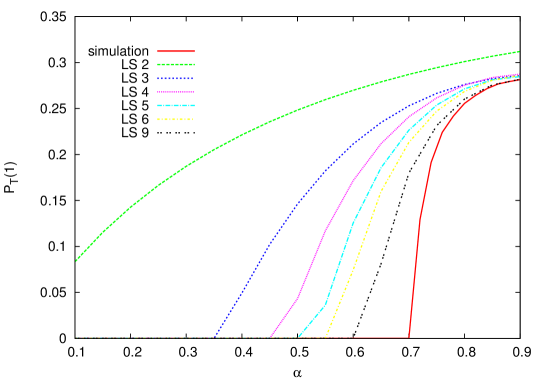
Figure 1: Graph of $P_{T}(1)$ for $T=10^{4}$ as a function $\alpha$ for probabilistic CA rule defined in eq. (6). Continuous line represents values of $P_{T}(1)$ obtained by Monte Carlo simulations, and dashed lines values of $Q_{T}(1)$ obtained by iterating local structure maps of level $k=2,3,4,5$ and $9$.

For some simple CA rules, the local structure approximation is exact. Such is the case of idempotent rules, that is, CA rules for which $F^{2}=F$. Gutowitz et al (1987) found that this is also the case for what he calls linear rules, toggle rules, and asymptotically trivial rules.

7 Exact calculations of probabilities of short blocks along the orbit

If approximations provided by the local structure theory are not enough, one can attempt to compute orbits of Bernoulli measures exactly. Typically, it is not possible to obtain expressions for all block probabilities $P_{n}(\mathbf{a})$ along the orbit, yet one can often compute $P_{n}(\mathbf{a})$ if $\mathbf{a}$ is short, for example, containing just one, two, or three symbols.

For elementary CA rules, the behaviour of $P_{n}(1)$ as a function of $n$ has been studied extensively by many authors, starting from Wolfram (1983), who determined numerical values of $P_{\infty}(1)$ for a wide class of CA rules and postulated exact values for some of them. Later one exact values of $P_{n}(1)$ have been established for some elementary rules, and in some cases, $P_{n}(\mathbf{a})$ has been computed for all $|\mathbf{a}|\leq 3$. We will discuss these results in what follows.

When the rule is deterministic, transition probabilities in eq. (53) take values in the set $\{0,1\}$. Let us consider elementary cellular automata, that is, binary rules for which $N=1$, ${\mathcal{A}}=\{0,1\}$ and the radius $r=1$. For such rules, define the local function $f$ by $f(x_{1},x_{2},x_{3})=w(1|x_{1}x_{2}x_{3})$ for all $x_{1},x_{2},x_{3}\in\{0,1\}$. Elementary CA with the local local function $f$ are usually identified by their Wolfram number $W(f)$, defined as (Wolfram, 1983)

$$W(f)=\sum_{x_{1},x_{2},x_{3}=0}^{1}f(x_{1},x_{2},x_{3})2^{(2^{2}x_{1}+2^{1}x_{2}+2^{0}x_{3})}.$$

A block evolution operator corresponding to $f$ is a mapping ${\mathbf{f}}:\mathcal{A}^{\star}\mapsto\mathcal{A}^{\star}$ defined as follows. Let $a=a_{0}a_{1}\ldots a_{n-1}\in\mathcal{A}^{n}$ where $n\geq 3$. Then

$${\mathbf{f}}(a)=\{f(a_{i},a_{i+1},a_{i+2})\}_{i=0}^{n-3}.$$ (77)

For elementary CA eq. (53) reduces to

$$(F\mu)([\mathbf{a}])=\sum_{\mathbf{b}\in{\mathbf{f}}^{-1}(\mathbf{a})}\mu([\mathbf{b}]),$$ (78)

where we dropped indices indicating where the cylinder set is anchored (we assume shift-invariance of measure $\mu$), and where ${\mathbf{f}}^{-1}(\mathbf{a})$ is the set of preimages of $\mathbf{a}$ under the block evolution operator ${\mathbf{f}}$. This can be generalized to the $n$-th iterate of $F$,

$$P_{n}(\mathbf{a})=(F^{n}\mu)([\mathbf{a}])=\sum_{\mathbf{b}\in{\mathbf{f}}^{-n}(\mathbf{a})}\mu([\mathbf{b}]),$$ (79)

where, again, ${\mathbf{f}}^{-n}(\mathbf{a})$ is the set of preimages of $\mathbf{a}$ under ${\mathbf{f}}^{n}$, the $n$-th iterate of ${\mathbf{f}}$. Thus, if we know the elements of the set of $n$-step preimages of the block $\mathbf{a}$ under the block evolution operator ${\mathbf{f}}$, then we can easily compute the probability $P_{n}(\mathbf{a})$.

Now, let us suppose that the initial measure is a Bernoulli measure $\mu_{p}$, defined by $\mu_{p}([\mathbf{a}])=p^{\#_{1}(\mathbf{a})}(1-p)^{\#_{0}(\mathbf{a})}$, where $\#_{s}(\mathbf{a})$ denotes number of symbols $s$ in $\mathbf{a}$ and where $p\in[0,1]$ is a parameter. In such a case eq. (79) reduces to

$$P_{n}(\mathbf{a})=\sum_{\mathbf{b}\in{\mathbf{f}}^{-n}(\mathbf{a})}p^{\#_{1}(\mathbf{b})}(1-p)^{\#_{0}(\mathbf{b})}.$$ (80)

Furthermore, if $p=1/2$, then the above reduces to even simpler form,

$$P_{n}(\mathbf{a})=\sum_{\mathbf{b}\in{\mathbf{f}}^{-n}(\mathbf{a})}\frac{1}{2^{|\mathbf{b}|}}=\frac{\mathop{\mathrm{card}}{\mathbf{f}}^{-n}(\mathbf{a})}{2^{|\mathbf{a}|+2n}}.$$ (81)

For many elementary CA rules and for short blocks $\mathbf{a}$, the sets ${\mathbf{f}}^{-n}(\mathbf{a})$ exhibit simple enough structure to be described and enumerated by combinatorial methods, so that the formula for $\mathop{\mathrm{card}}{\mathbf{f}}^{-n}$ can be constructed and/or the sum in eq. (80) can be computed. Although there is no precise definition of “simple enough structure”, the known cases can be informally classified into five groups:

1. rules with preimage sets that are “balanced” (have the same number of preimages for each block),

2. rules with preimage sets mostly composed of long blocks of identical symbols (having long runs) or long blocks of arbitrary symbols,

3. rules with preimage sets that can be described as sets of strings in which some local property holds everywhere,

4. rules with preimage sets that can be described as strings in which some global (non-local) property holds,

5. rules for which preimage sets are related to preimage sets of some known solvable rule.

Selection of the most interesting examples in each category is given below.

7.1 Balanced preimages: surjective rules

It is well known that the symmetric Bernoulli measure $\mu_{1/2}$ is invariant under the action of a surjective rule (see Pivato, 2009, and references therein). In one dimension, surjectivity is a decidable property, and the relevant algorithm is known, due to Amoroso and Patt (1972). Among elementary CA rules, surjective rules have the following Wolfram numbers: 15, 30, 45, 51, 60, 90, 105, 106, 150, 154, 170 and 204. For all of them, for the initial measure $\mu=\mu_{1/2}$ and for any block $\mathbf{a}$,

$$P_{n}(\mathbf{a})=2^{-|\mathbf{a}|}.$$ (82)

The above result is a direct consequence of the Balance Theorem, first proved by Hedlund (1969), which states that for a surjective rule, $\mathop{\mathrm{card}}{\mathbf{f}}^{-1}(\mathbf{a})$ is the same for all blocks $\mathbf{a}$ of a given length. For elementary rules this implies that $\mathop{\mathrm{card}}{\mathbf{f}}^{-1}(\mathbf{a})=4$, and, therefore, $\mathop{\mathrm{card}}{\mathbf{f}}^{-n}(\mathbf{a})=4^{n}$. From eq. (81) one then obtains eq. (82).

7.2 Preimages with long runs and arbitrary symbols: rule 130

Consider the elementary CA with the local function

$$f\big{(}x_{1},x_{2},x_{3}\big{)}=\left\{\begin{array}[]{l l}1&\quad\text{if}\quad(x_{1}\;x_{2}\;x_{3})=(0\;0\;1)\text{ or }(1\;1\;1),\\ 0&\quad\text{otherwise,}\\ \end{array}\right.$$ (83)

Its Wolfram number is $W(f)=130$, and we will refer to it as simply “rule 130”. Subsequently, any rule with Wolfram number $W(f)$ will be referred to as “rule $W(f)$”. For rule 130 and for $\mu_{p}$, the the probabilities $P_{n}(\mathbf{a})$ are known for $|\mathbf{a}|\leq 3$ (Fukś and Skelton, 2010). The corresponding formulae are rather long, thus we give only the expression for $P_{n}(0)$.

$$P_{n}(0)=1-p^{2n+1}-\frac{p\,\left(-{p}^{4\lceil(n-2)/2\rceil+4}+{p}^{4\lceil(n-2)/2\rceil+5}-{p}^{4\lfloor n/2\rfloor+3}+{p}^{3}-p+1\right)}{{p}^{3}+{p}^{2}+p+1}.$$ (84)

The above result is based on the fact that for rule 130, the set ${\mathbf{f}}^{-n}(111)$ has only one element, namely the block $11\ldots 1$, hence $\mathop{\mathrm{card}}{\mathbf{f}}^{-n}(111)=1$. Moreover, the set ${\mathbf{f}}^{-n}(001)$ consists of all blocks of the form

$$\underbrace{\star\ldots\star}_{2n-2i}\;1\;0\;1\;\underbrace{1\ldots 1}_{2i}\quad\text{(if $i$ is odd)}\quad\quad\text{or}\quad\quad\underbrace{\star\ldots\star}_{2n-2i}\;0\;0\;1\;\underbrace{1\ldots 1}_{2i}\quad\text{(if $i$ is even),}$$

where $i\in\{0\dots n\}$ and $\star$ denotes an arbitrary value in $\mathcal{A}$. Probabilities of occurence of blocks 111 and 001 can thus be easily computed. Using the fact that for this rule $P_{n}(0)=1-P_{n-1}(111)-P_{n-1}(001)$, one then obtains eq. (84). The floor and ceiling operators appear in that formula because different expressions are needed for odd and even $n$, as it is evident from the structure of preimages of 001 described above. Rule 130 is an example of a rule where convergence of $P_{n}(0)$ to its limiting value is essentially exponential (like in rule 172 discussed below, except that there are some small variations between values corresponding to even and odd $n$.

7.3 Preimages described by a local property: rule 172

The local function of rule 172 is defied as

$$f(x_{1},x_{2},x_{3})=\left\{\begin{array}[]{ll}x_{2}&\mbox{if $x_{1}=0$,}\\ x_{3}&\mbox{if $x_{1}=1$.}\end{array}\right.$$ (85)

The combinatorial structure of ${\mathbf{f}}^{-n}(\mathbf{a})$ for this rule can be described, for some blocks $\mathbf{a}$, as binary strings with forbidden sub-blocks. More precisely, one can prove the following proposition (Fukś, 2010).

Proposition 4

Block $\mathbf{b}$ of length $2n+1$ belongs to ${\mathbf{f}}^{-n}(1)$ for rule 172 if and only if it has the structure $\mathbf{b}=\underbrace{\star\star\ldots\star}_{n-2}001\underbrace{\star\star\ldots\star}_{n}$, or $\mathbf{b}=\underbrace{\star\star\ldots\star}_{n-2}a_{1}a_{2}\ldots a_{n+1}c_{1}c_{2}$, where $a_{1}a_{2}\ldots a_{n}$ is a binary string which does not contain any pair of adjacent zeros, and

$$c_{1}c_{2}=\begin{cases}1\star,&\text{if}\,\,\,a_{n+1}=0,\\ \star 1,&\text{otherwise}.\end{cases}$$ (86)

Since the number of binary strings of length $n$ without any pair of consecutive zeros is know to be $F_{n+2}$, where $F_{n}$ is the $n$-th Fibonacci number, it is not surprising that Fibonacci numbers appear in expressions for block probabilities of rule 172. For this rule and $\mu=\mu_{1/2}$, probabilities $P_{n}(\mathbf{a})$ are known for $|\mathbf{a}|\leq 3$, as shown below.

$$P_{n}(0) =\frac{7}{8}-\frac{F_{n+3}}{2^{n+2}},$$ (87)

$$P_{n}(00) ={3}/{4}-{2}^{-n-2}F_{n+3}-{2}^{-n-4}F_{n+2},$$

$$P_{n}(000) ={5}/{8}-{2}^{-n-2}F_{n+3}-{2}^{-n-4}F_{n+2},$$

$$P_{n}(010) ={1}/{8}-{2}^{-n-3}F_{n+1},$$

Note that the above are probabilities in short block representation, thus all remaining probabilities of blocks of length up to 3 can be obtained using eq. (44). More recently, $P_{n}(0)$ has been computed for arbitrary $\mu_{p}$ (Fukś, 2016b),

$$P_{n}(0)=1-(1-p)^{2}p-\frac{p^{2}}{\lambda_{2}-\lambda_{1}}\left(\alpha_{1}\lambda_{1}^{n-1}+\alpha_{2}\lambda_{2}^{n-1}\right),$$ (88)

where

$$\lambda_{1,2} =\frac{1}{2}p\pm\frac{1}{2}\sqrt{p(4-3p)},$$ (89)

$$\alpha_{1,2} =\left(\frac{p}{2}-1\right)\sqrt{p\left(4-3\,p\right)}\pm\left(\frac{p^{2}}{2}-1\right).$$ (90)

7.4 Preimages described by a non-local property: rule 184

While in rule 172 the ombinatorial description of sets ${\mathbf{f}}^{-n}(\mathbf{a})$ involved some local conditions (e.g., two consecutive zeros are forbidden), in rule 184, with the local function $f(x_{1},x_{2},x_{3})=x_{1}+x_{2}x_{3}-x_{1}x_{2}$, the conditions are more of a global nature, that is, involving properties of longer substrings. In particular, one can show the following.

Proposition 5

The block $b_{1}b_{2}\ldots b_{2n+2}$ belongs to ${\mathbf{f}}^{-n}(00)$ under rule $184$ if and only if $b_{1}=0$, $b_{2}=0$ and $2+\sum_{i=3}^{k}\xi(b_{i})>0$ for every $3\leq k\leq 2n+2$, where $\xi(0)=1$, $\xi(1)=-1$.

Proof of this property relies on the fact that rule 184 is known to be equivalent to a ballistic annihilation process (Krug and Spohn, 1988; Fukś, 1999; Belitsky and Ferrari, 2005). Another crucial property of rule 184 is that it is number-conserving, that is, conserves the number of zeros and ones. Using this fact and the above proposition, probabilities $P_{n}(\mathbf{a})$ can be computed for for $\mu_{p}$ and $|\mathbf{a}|\leq 2$,

$$P_{n}(0)=1-p,\,\,\,\,\,P_{n}(00)=\sum_{j=1}^{n+1}\frac{j}{n+1}{{2n+2}\choose{n+1-j}}p^{n+1-j}(1-p)^{n+1+j}.$$ (91)

The main idea which is used in deriving the above expression is the fact that preimage sets ${\mathbf{f}}^{-1}(00)$ have a similar structure to trajectories of one-dimensional random walk starting from the origin and staying on the positive semi-axis. Enumeration of such trajectories is a well known combinatorial problem, and the binomial coefficient appearing in the expression for $P_{n}(00)$ indeed comes from this enumeration procedure. In the limit of large $n$ one can demonstrate that

$$\lim_{n\rightarrow\infty}P_{n}(00)=\left\{\begin{array}[]{ll}1-2p&\mbox{if $p<1/2$},\\ 0&\mbox{otherwise}.\end{array}\right.$$ (92)

All the above results can be extended to generalizations of rule 184 with larger radius (Fukś, 1999).

A special case of $\mu_{1/2}$ is especially interesting, as in this case probabilities of blocks up to length 3 can be obtained,

$$P_{n}(0) =\frac{1}{2},$$ (93)

$$P_{n}(00) ={2}^{-2-2\,n}{2\,n+1\choose n+1},$$ (94)

$$P_{n}(000) ={2}^{-2\,n-3}{2\,n+1\choose n+1},$$ (95)

$$P_{n}(010) =\frac{1}{2}-3\cdot{2}^{-3-2\,n}{2\,n+1\choose n+1}.$$ (96)

Using Stirling’s approximation for factorials for large $n$, one obtains $P_{n}(00)\sim n^{-1/2}$, thus $P_{n}(00)$ converges to $0$ as a power law with exponent $1/2$.

7.5 Preimage sets related to preimages of other solvable rules: rule 14

The local function of rule 14 is defied by $f(0,0,1)=f(0,1,0)=f(0,1,1)=1$, and $f(x_{0},x_{1},x_{2})=0$ for all other triples $(x_{0},x_{1},x_{2})\in\{0,1\}^{3}$. For rule 14 and $\mu=\mu_{1/2}$, the probabilities $P_{n}(\mathbf{a})$ are known for $|\mathbf{a}|\leq 3$, and are given by

$$P_{n}(0) =\frac{1}{2}\left(1+\frac{2n-1}{4^{n}}C_{n-1}\right),$$ (97)

$$P_{n}(00) ={2}^{-2-2\,n}(n+1)C_{{n}}+\frac{1}{4},$$ (98)

$$P_{n}(000) =2^{-2n-3}\left(4\,n+3\right)C_{n},$$ (99)

$$P_{n}(010) ={2}^{-2-2\,n}\left(n+1\right)C_{{n}},$$ (100)

where $C_{n}$ is the $n$-th Catalan number (Fukś and Haroutunian, 2009). These formulae were obtained using the fact that this rule conserves the number of blocks 10 and that the combinatorial structure of preimage sets of some short blocks resembles the structure of related preimage sets under the rule 184. More precisely, computation of the above block probabilities relies on the following property (see ibid. for proof).

Proposition 6

For any $n\in{\mathbbm{N}}$, the number of $n$-step preimages of 101 under the rule 14 is the same as the number of $n$-step preimages of 000 under the rule 184, that is,

$$\mathop{\mathrm{card}}{\mathbf{f}}^{-n}_{14}(101)=\mathop{\mathrm{card}}{\mathbf{f}}^{-n}_{184}(000),$$ (101)

where subscripts 184 and 14 indicate block evolution operators for, respectively, CA rules 184 and 14. Moreover, the bijection $M_{n}$ from the set ${\mathbf{f}}^{-n}_{184}(000)$ to the set ${\mathbf{f}}^{-n}_{14}(101)$ is defined by

$$M_{n}(x_{0}x_{1}\ldots x_{m})=\left\{n+j+1+\sum_{i=0}^{j}x_{i}\mod 2\right\}_{j=0}^{m}$$ (102)

for $m\in{\mathbbm{N}}$ and for $x_{0}x_{1}\ldots x_{m}\in\{0,1\}^{m}$.

As in the case of rule 184, one can show that for rule 14 and large $n$,

$$P_{n}(0)\approx\frac{1}{2}+\frac{1}{4\sqrt{\pi}}n^{-\frac{1}{2}}.$$ (103)

The power law which appears here exhibits the same exponent as in the case of rule 184 for $P_{n}(00)$.

7.6 Convergence of block probabilities

The examples shown in the previous sections indicate that in all cases for which $P_{n}(\mathbf{a})$ can be computed exactly, as $n\to\infty$, $P_{n}(\mathbf{a})$ remains either constant, or converges to its limiting value exponentially or as a power law. The exponential convergence is the most prevalent. Indeed, for many other elementary CA rules for which formulae for $P_{n}(0)$ are either known or conjectured, the exponential convergence to $P_{\infty}(0)$ can be observed most frequently. This includes 15 elementary rules which are known as asymptotic emulators of identity (Rogers and Want, 1994; Fukś and Soto, 2014). Formulae for $P_{n}(1)$ for the initial measure $\mu_{1/2}$ for these rules are shown below. Starred rules are those for which a formal proof has been published in the literature (see Fukś and Soto, 2014, and references therein).

• Rule $13$: $P_{n}(1)=7/16-(-2)^{-n-3}$

• Rule $32^{\star}$: $P_{n}(1)=2^{-1-2n}$

• Rule $40$: $P_{n}(1)=2^{-n-1}$

• Rule $44$: $P_{n}(1)=1/6+\frac{5}{6}2^{-2n}$

• Rule $77^{\star}$: $P_{n}(1)=1/2$

• Rule $78$: $P_{n}(1)=9/16$

• Rule $128^{\star}$: $P_{n}(1)=2^{-1-2n}$

• Rule $132^{\star}$: $P_{n}(1)=1/6+\frac{1}{3}2^{-2n}$

• Rule $136^{\star}$: $P_{n}(1)=2^{-n-1}$

• Rule $140^{\star}$: $P_{n}(1)=1/4+2^{-n-2}$

• Rule $160^{\star}$: $P_{n}(1)=2^{-n-1}$

• Rule $164$: $P_{n}(1)=1/12-\frac{1}{3}4^{-n}+\frac{3}{4}2^{-n}$

• Rule $168^{\star}$: $P_{n}(1)=3^{n}2^{-2n-1}$

• Rule $172^{\star}$: $P_{n}(1)=\frac{1}{8}+\frac{(10-4\sqrt{5})(1-\sqrt{5})^{n}+(10+4\sqrt{5})(1+\sqrt{5})^{n}}{40\cdot 2^{2n}}$

• Rule $232$: $P_{n}(1)=1/2$

The formula for rule 172, included here for completeness, can obviously be obtained from eq. (87) by using explicit expressions for Fibonacci numbers in terms of powers of the golden ratio.

Power laws appearing in rules 184 and 14, as mentioned already, are a result of the fact that dynamics of these rules can be understood as a motion of deterministic “particles” propagating in a regular background. The same type of “defect kinematics” has been observed, among other elementary CA rules, in rule 18 (Grassberger, 1984), for which

$$P_{n}(11)\sim n^{-1/2}.$$

The above power law can be explained by the fact that in rule 18 one can view sequences of 0’s of even length as “defects” which perform a random walk and annihilate upon collision, as discovered numerically by Grassberger (1984) and later formally demonstrated by Eloranta and Nummelin (1992). A very general treatment of particle kinematics in CA confirming this result can be found in the work of Pivato (2007).

Another example of an interesting power law appears in rule 54, for which Boccara et al (1991) numerically verified that

$$P_{n}(1)\sim n^{-\gamma},$$

where $\gamma\approx 0.15$. Particle kinematics of rule 54 is now very well understood (Pivato, 2007), but the above power law has not been formally demonstrated, and the exact value of the exponent $\gamma$ remains unknown.

8 Examples of exact results for probabilistic CA rules

For probabilistic rules, one cannot use eq. (80) because the block evolution operator $\mathbf{f}^{-n}$ does not have any obvious non-deterministic version. Once thus has to work directly with eq. (53).

Equation (53) can be written for the $n$-th iterate of $F$,

$$(F^{n}\mu)([\mathbf{a}]_{i})=\sum_{\mathbf{b}\in\mathcal{A}^{|\mathbf{a}|+2nr}}w^{n}(\mathbf{a}|\mathbf{b})\mu([\mathbf{b}]_{i-nr})\mathrm{\,\,for\,\,all\,\,}i\in\mathbb{Z},\mathbf{a}\in\mathcal{A}^{\star},$$ (104)

where we define the $n$-step block transition probability $w^{n}$ recursively, so that, when $n\geq 2$ and for any blocks $c\mathbf{a}\in{\mathcal{A}}^{\star}$ and $\mathbf{b}\in{\mathcal{A}}^{|\mathbf{a}|+2rn}$,

$$w^{n}(\mathbf{a}|\mathbf{b})=\sum_{\mathbf{b}^{\prime}\in{\mathcal{A}}^{|\mathbf{a}|+2r(n-1)}}w^{n-1}(\mathbf{a}|\mathbf{b}^{\prime})w(\mathbf{b}^{\prime}|\mathbf{b}).$$ (105)

The $n$-step block transition probability $w^{n}(\mathbf{a}|\mathbf{b})$ can be intuitively understood as the conditional probability of seeing the block $\mathbf{a}$ after $n$ iterations of $F$, conditioned on the fact that the original configuration contained the block $\mathbf{b}$.

Using definition of $w$ given in eq. (54), one can produce an explicit formula for $w^{n}$,

$$w^{n}(\mathbf{a}|\mathbf{b})=\sum_{\begin{subarray}{c}\mathbf{b}_{n-1}\in{\mathcal{A}}^{|\mathbf{a}|+2r(n-1)}\vspace{-1.5mm}\\ \vdots\vspace{0.5mm}\\ \mathbf{b}_{1}\in\mathcal{A}^{|\mathbf{a}|+2r}\end{subarray}}w(\mathbf{a}|\mathbf{b}_{1})\left(\prod_{i=1}^{n-2}w(\mathbf{b}_{i}|\mathbf{b}_{i+1})\right)w(\mathbf{b}_{n-1}|\mathbf{b}).$$ (106)

For a shift-invariant initial probability measure $\mu$, equation (104) becomes

$$P_{n}(\mathbf{a})=\sum_{\mathbf{b}\in\mathcal{A}^{|\mathbf{a}|+2nr}}w^{n}(\mathbf{a}|\mathbf{b})P_{0}(\mathbf{b}).$$ (107)

Since some of the transition probabilities may be zero, we define, for any block $\mathbf{b}\in\mathcal{A}^{\star}$,

$$\mathop{\rm{supp}}w^{n}(\mathbf{a}|\cdot)=\{\mathbf{b}\in\mathcal{A}^{|\mathbf{a}+2nr}:w^{n}(\mathbf{a}|\mathbf{b})>0\},$$ (108)

and then we have

$$P_{n}(\mathbf{a})=\sum_{\mathbf{b}\in\mathop{\rm{supp}}w^{n}(\mathbf{a}|\cdot)}w^{n}(\mathbf{a}|\mathbf{b})P_{0}(\mathbf{b}).$$ (109)

In some cases, $\mathop{\rm{supp}}w^{n}(\mathbf{a}|\cdot)$ is small and has a simple structure, and the needed $w^{n}(\mathbf{a}|\mathbf{b})$ can be computed directly from eq. (106). This approach has been successfully used for a class of probabilistic CA rules known as $\alpha$-asynchronous rules with single transitions (Fukś and Skelton, 2011a). We show two examples of such rules below.

8.1 Rule 200A

Rule 200A, known as $\alpha$-asynchronous rule 200, is defined by transition probabilities

$$w(1|\mathbf{b})=\begin{cases}0&\quad\text{if\;}\mathbf{b}\in\{000,001,100,101\},\\ 1&\quad\text{if\;}\mathbf{b}\in\{011,110,111\},\\ 1-\alpha&\quad\text{if\;}\mathbf{b}=010,\end{cases}$$ (110)

and $w(0|\mathbf{b})=1-w(1|\mathbf{b})$ for all $\mathbf{b}\in\{0,1\}^{3}$, where $\alpha\in[0,1]$ is a parameter. The set $\mathop{\rm{supp}}w^{n}(1|\cdot)$ for this rule consists of all blocks of the form

$$\underbrace{\star\;\cdots\;\star\;}_{n}\;1\;\underbrace{\star\;\cdots\;\star}_{n}.$$ (111)

Moreover, one can show that for any block $\mathbf{b}\in\mathop{\rm{supp}}w^{n}(1|\cdot)$ where the central 1 has 0s as both neighbours, $w^{n}(1|\mathbf{b})=(1-\alpha)^{n}$, while $w^{n}(1|\mathbf{b})=1$ for all other cases. This allows to compute $P_{n}(1)$ and $P_{n}(0)$ from eq. (109) directly. By the same method probabilities of other blocks of length up to 3 can be computed for rule 200A and $\mu_{p}$, and results are shown below.

$$P_{n}(0) =1-{p}^{2}\left(2-p\right)-\left(1-p\right)^{n}p\,\left(1-p\right)^{2},$$ (112)

$$P_{n}(00) =-\left(-1+p\right)^{2}\left(-2\,p+2\,\left(1-\alpha\right)^{n}p-1\right),$$

$$P_{n}(000) =-{p}^{2}\left(-1+p\right)^{3}\left(1-\alpha\right)^{2\,n}+p\,\left(2\,{p}^{2}-3\right)\left(-1+p\right)^{2}\left(1-\alpha\right)^{n}$$

$$-\left({p}^{3}+{p}^{2}-2\,p-1\right)\left(-1+p\right)^{2},$$

$$P_{n}(010) =\left(1-\alpha\right)^{n}p\,\left(1-p\right)^{2}.$$

Exponential convergence toward limiting values can clearly be observed in all of these block probabilities.

8.2 Rule 140A

Another example is rule 140A, defined as

$$w(1|\mathbf{b})=\begin{cases}0&\quad\text{if\;}\mathbf{b}\in\{000,001,100,101\},\\ 1&\quad\text{if\;}\mathbf{b}\in\{010,011,111\},\\ 1-\alpha&\quad\text{if\;}\mathbf{b}=110,\end{cases}$$ (113)

and $w(0|\mathbf{b})=1-w(1|\mathbf{b})$ for all $\mathbf{b}\in\{0,1\}^{3}$. For this rule the set $\mathop{\rm{supp}}w^{n}(1|\cdot)$ has the same structure as for rule 200A, except that the values of $w^{n}(1|\mathbf{b})$ are different. For blocks $\mathbf{b}\in\mathcal{A}^{2n+1}$ having the structure

$$\underbrace{\star\;\cdots\;\star\;}_{n-1}1\quad\underline{1}\quad\underbrace{1\;\cdots\;1}_{k-1}\;0\;\underbrace{\star\;\cdots\;\star}_{n-k},$$ (114)

where $0\leq k-1\leq n$, it has been demonstrated (Fukś and Skelton, 2011a) that

$$w^{n}(1|\mathbf{b})=\begin{cases}\beta^{n}&\quad\text{if }k=1,\\ \beta^{n}\left(\frac{\alpha}{\beta}\right)^{k-1}\binom{n-1}{k-1}+\beta^{n-k+1}\sum_{j=0}^{k-2}\limits\binom{n-k+j}{j}\alpha^{j}&\quad\text{if }2\leq k\leq n,\\ 1&\quad\text{if }k=n+1.\end{cases}$$ (115)

For all other blocks in $\mathop{\rm{supp}}w^{n}(1|\cdot)$ one has $w^{n}(1|\mathbf{b})=1$. Using this result, probability $P_{n}(0)$ can be computed assuming initial measure $\mu_{p}$, although the summation in eq. (104) is rather complicated. The end result, shown below, is nevertheless surprisingly simple.

$$P_{n}(0)=1-\rho(1-\rho)-\rho^{2}\left(1-(1-\rho)\alpha\right)^{n}.$$ (116)

Corresponding formulae for $P_{n}(\mathbf{a})$ for all $|\mathbf{a}|\leq 3$ have been constructed as well, but are omitted here.

8.3 Complete sets

Another case when eq. (56) becomes solvable is when there exists a subset of blocks which is called complete. A set of words $\mathcal{A}^{\star}\supset C=\{\mathbf{a}_{1},\mathbf{a}_{2},\mathbf{a}_{3},\ldots\}$ is complete with respect to a CA rule $F$ if for every $\mathbf{a}\in C$ and $n\in\mathbb{N}$, $P_{n+1}(\mathbf{a})$ can be expressed as a linear combination of $P_{n}(\mathbf{a}_{1}),P_{n}(\mathbf{a}_{2}),P_{n}(\mathbf{a}_{3}),\ldots$. In this case, one can write eqs. (56) for blocks of the complete set only, and the right hand sides of them will also only include probabilities of blocks from the complete set. This way, a well-posed system of recurrence equations is obtained, and (at least in principle) it should be solvable.

This approach has been recently applied to a probabilistic CA rule defined by

$$w(1|000) =0,\,w(1|001)=\alpha,\,w(1|010)=1,\,w(1|011)=1,$$ (117)

$$w(1|100) =\beta,\,w(1|101)=\gamma,\,w(1|110)=1,\,w(1|111)=1,$$

and $w(0|b)=1-w(1|b)$ for all $b\in\{0,1\}^{3}$, where $\alpha,\beta,\gamma\in[0,1]$ are fixed parameters. This rule can be viewed as a generalized simple model for diffusion of innovations on one-dimensional lattice (Fukś, 2016a). The complete set for this rule consists of blocks $101$, $1001$, $100001$, $\ldots$. Equations (56) for blocks of the complete set simplify to

$$P_{n+1}(101)=(1-\gamma)P_{n}(101)+(\alpha-2\alpha\beta+\beta)P_{n}(1001)+\alpha\beta P_{n}(10001),$$ (118)

and, for $k>1$,

$$P_{n+1}(10^{k}1)=(1-\alpha)(1-\beta)P_{n}(10^{k}1)+(\alpha-2\alpha\beta+\beta)P_{n}(10^{k+1}1)+\alpha\beta P_{n}(10^{k+2}1).$$ (119)

The above equations can be solved, and, using the cluster expansion formula (Stauffer and Aharony, 1994),

$$P_{n}(0)=\sum_{k=1}^{\infty}kP_{n}(10^{k}1),$$ (120)

one obtains, assuming that the initial measure is $\mu_{p}$,

$$P_{n}(0)=\begin{cases}E\left(\left({p}\,\beta-1\right)\left({p}\,\alpha-1\right)\right)^{n}+F\left(1-\gamma\right)^{n}&\text{if }\alpha\beta p^{2}-(\alpha+\beta)p+\gamma\neq 0,\\ (G+Hn)(1-\gamma)^{n-1}&\text{if }\alpha\beta p^{2}-(\alpha+\beta)p+\gamma=0,\end{cases}$$ (121)

where $E,F,G,H$ are constants depending on parameters $\alpha,\beta,\gamma$ and $p$ (for detailed formulae, see Fukś, 2016a). For $\alpha\beta p^{2}-(\alpha+\beta)p+\gamma=0$, this is an example of a linear-exponential convergence of $P_{n}(0)$ toward its limiting value, the only one known for a binary rule.

9 Future directions

Both approximate and exact methods for computing orbits of Bernoulli measures under the action of cellular automata need further development.

Regarding approximate methods, although some simple classes of CA rules for which local structure approximation becomes exact are known, it is not known if there exist any wider classes of non-trivial rules for which this would be the case. This is certainly an area which needs further research. There seems to be some evidence that orbits of many deterministic rules possessing additive invariants are very well approximated by local structure theory, but no general results are known.

Regarding exact methods, the situation is similar. Although methods for computing exact values of $P_{n}(\mathbf{a})$ presented here are applicable to many different rules, it is still not clear if they are applicable to some wider classes of CA in general. Some such classes has been proposed, but formal results are still lacking. For example, there is a number of rules for which convergence of $P_{n}(1)$ to its limiting value $P_{\infty}(1)$ is known to be exponential, and it has been conjectured that for all rules known as asymptotic emulators of identity this is indeed the case. However, there seems to be some recent evidence that for rule 164, which belongs to asymptotic emulators of identity, the convergence is not exactly exponential (A. Skelton, private communication). Are then other classes of CA rules for which the convergence is always exponential? And, more importantly, are there any wide classes of non-trivial CA for which exact formulae for probabilities of short block are obtainable?

Another interesting question is the relationship between exact orbits of CA rules and approximate orbits obtained by iterating local structure maps. Which features or exact orbits are “inherited” by approximate orbits? It seems that often existence of additive invariants is “inherited” by local structure maps, yet more work in this direction is needed. On a related note, such behavior of $P_{n}(1)$ as observed in rules 172 or 140A (discussed earlier in this article) strongly resembles hyperbolicity in finitely-dimensional dynamical systems. Hyperbolic fixed points are common type of fixed points in dynamical systems. If the initial value is near the fixed point and lies on the stable manifold, the orbit of the dynamical system converges to the fixed point exponentially fast. One could argue that the exponential convergence to $P_{\infty}(1)$ observed in such rules as rule 172 or 140A is somewhat related to finitely-dimensional hyperbolicity. Since local structure maps which approximate dynamics of a given CA are finitely-dimensional, one could ask what is the nature of their fixed points – are these hyperbolic for CA exhibiting hyperbolic-like dynamics? Is hyperbolicity of orbits of CA rules somewhat “inherited” by local structure maps? If so, under what conditions does this happen? All those questions need to be investigated in details in future years.

Finally, one should mention that both theoretical developments and examples presented in this article pertain to one-dimensional cellular automata. Higher-dimensional systems have been studied in the context of the local structure theory (Gutowitz and Victor, 1987), and some examples or two-dimensional cellular automata with exact expressions for small block probabilities are known (Fukś and Skelton, 2011b), yet the orbits of Bernoulli measures under higher-dimensional CA are still mostly an unexplored terrain. Given the importance of two- and threepice -dimensional CA in applications, this subject will likely attract some attention in the near future.

References

- Amoroso and Patt (1972) Amoroso S, Patt YN (1972) Decision procedures for surjectivity and injectivity of parallel maps for tesselation structures. Journal of Computer and System Sciences 6:448–464
- Belitsky and Ferrari (2005) Belitsky V, Ferrari PA (2005) Invariant measures and convergence properties for cellular automaton 184 and related processes
- Boccara et al (1991) Boccara N, Nasser J, Roger M (1991) Particlelike structures and their interactions in spatiotemporal patterns generated by one-dimensional deterministic cellular-automaton rules. Phys Rev A 44:866–875
- Brascamp (1971) Brascamp HJ (1971) Equilibrium states for a one dimensional lattice gas. Communications In Mathematical Physics 21(1):56
- Eloranta and Nummelin (1992) Eloranta K, Nummelin E (1992) The kink of cellular automaton rule 18 performs a random walk. Journal of Statistical Physics 69(5):1131–1136
- Fannes and Verbeure (1984) Fannes M, Verbeure A (1984) On solvable models in classical lattice systems. Commun Math Phys 96:115–124
- Fatès (2009) Fatès N (2009) Asynchronism induces second order phase transitions in elementary cellular automata. Journal of Cellular Automata 4(1):21–38, URL http://hal.inria.fr/inria-00138051
- Formenti and Kůrka (2009) Formenti E, Kůrka P (2009) Dynamics of cellular automata in non-compact spaces. In: Meyers RA (ed) Encyclopedia of Complexity and System Science, Springer
- Fukś (1999) Fukś H (1999) Exact results for deterministic cellular automata traffic models. Phys Rev E 60:197–202, DOI 10.1103/PhysRevE.60.197, arXiv:comp-gas/9902001
- Fukś (2010) Fukś H (2010) Probabilistic initial value problem for cellular automaton rule 172. DMTCS proc AL:31–44, arXiv:1007.1026
- Fukś (2013) Fukś H (2013) Construction of local structure maps for cellular automata. J of Cellular Automata 7:455–488, arXiv:1304.8035
- Fukś (2016a) Fukś H (2016a) Computing the density of ones in probabilistic cellular automata by direct recursion. In: Louis PY, Nardi FR (eds) Probabilistic Cellular Automata - Theory, Applications and Future Perspectives, to appear in Lecture Notes in Computer Science, arXiv:1506.06655
- Fukś (2016b) Fukś H (2016b) Explicit solution of the cauchy problem for cellular automaton rule 172, in press
- Fukś and Haroutunian (2009) Fukś H, Haroutunian J (2009) Catalan numbers and power laws in cellular automaton rule 14. Journal of cellular automata 4:99–110, arXiv:0711.1338
- Fukś and Skelton (2010) Fukś H, Skelton A (2010) Response curves for cellular automata in one and two dimensions – an example of rigorous calculations. International Journal of Natural Computing Research 1:85–99, arXiv:1108.1987
- Fukś and Skelton (2011a) Fukś H, Skelton A (2011a) Orbits of Bernoulli measure in asynchronous cellular automata. Dis Math Theor Comp Science AP:95–112
- Fukś and Skelton (2011b) Fukś H, Skelton A (2011b) Response curves and preimage sequences of two-dimensional cellular automata. In: Proceedings of the 2011 International Conference on Scientific Computing: CSC-2011, CSERA Press, pp 165–171, arXiv:1108.1559
- Fukś and Soto (2014) Fukś H, Soto JMG (2014) Exponential convergence to equilibrium in cellular automata asymptotically emulating identity. Complex Systems 23:1–26, arXiv:1306.1189
- Grassberger (1984) Grassberger P (1984) Chaos and diffusion in deterministic cellular automata. Physica D 10(1):52–58
- Gutowitz and Victor (1987) Gutowitz HA, Victor JD (1987) Local structure theory in more than one dimension. Complex Systems 1:57–68
- Gutowitz et al (1987) Gutowitz HA, Victor JD, Knight BW (1987) Local structure theory for cellular automata. Physica D 28:18–48
- Hedlund (1969) Hedlund G (1969) Endomorphisms and automorphisms of shift dynamical systems. Mathematical Systems Theory 3:320–375
- Krug and Spohn (1988) Krug J, Spohn H (1988) Universality classes for deterministic surface growth. Phys Rev A 38:4271–4283
- Kůrka (2005) Kůrka P (2005) On the measure attractor of a cellular automaton. Discrete and Continuous Dynamical Systems pp 524 – 535
- Kůrka and Maass (2000) Kůrka P, Maass A (2000) Limit sets of cellular automata associated to probability measures. Journal of Statistical Physics 100:1031–1047
- McIntosh (2009) McIntosh H (2009) One Dimensional Cellular Automata. Luniver Press, Frome
- Pivato (2007) Pivato M (2007) Defect particle kinematics in one-dimensional cellular automata. Theoretical Computer Science 377(1):205–228
- Pivato (2009) Pivato M (2009) Ergodic theory of cellular automata. In: Meyers RA (ed) Encyclopedia of Complexity and System Science, Springer
- Rogers and Want (1994) Rogers T, Want C (1994) Emulation and subshifts of finite type in cellular automata. Physica D 70:396–414
- Stauffer and Aharony (1994) Stauffer D, Aharony A (1994) Introduction to percolation theory. Taylor and Francis
- Wolfram (1983) Wolfram S (1983) Statistical mechanics of cellular automata. Reviews of Modern Physics 55(3):601–644
Index
- “thick bar” fraction §5
- alphabet §2
- asymptotic emulators of identity §9
- asymptotically trivial rule §6
- Balance Theorem §7.1
- ballistic annihilation §7.4
- Bayesian approximation §5
- Bayesian extension §5
- Bernoulli measure §7
- block evolution operator §7
- block of symbols §2
- block probabilities §2
- Cantor metric §2
- Catalan numbers §7.5
- complete set §8.3
- consistency conditions §2
- cylinder set §2
- defect kinematics §7.6
- deterministic cellular automaton §4
- elementary cellular automata §7
- entropy density §5
- exponential convergence §7.6
- Fibonacci numbers §7.3
- finite block measure §5
- golden ratio §7.6
- Hahn-Kolmogorov theorem §2
- idempotent rule §6
- local function §7
- local structure approximation §5
- local structure map §6
- local structure theory §5
- local transition function §4
- long block representation §3
- Markov measure §5
- number-conserving rule §7.4
- power law convergence §7.4
- preimage set §7
- Probabilistic cellular automaton §4
- random walk §7.6
- scramble operator §5
- semi-algebra of elementary cylinder sets §2
- shift-invariant probability measure Theorem 1
- short block representation §3
- surjective cellular automata §7.1
- surjectivity §7.1
- symbol set §2
- toggle rule §6
- transition probabilities §4
- -algebra §2