Dynamics within a tunable harmonic/quartic waveguide

Abstract

We present an analytical solution to the dynamics of a noninteracting cloud of thermal atoms in a cigar-shaped harmonic trap with a quartic perturbation along the axial direction. We calculate the first and second moments of position, which are sufficient to characterize the trap. The dynamics of the thermal cloud differ notably from those of a single particle, with an offset to the oscillation frequency that persists even as the oscillation amplitude approaches zero. We also present some numerical results that describe the effects of time-of-flight on the behavior of the cloud in order to better understand the results of a hypothetical experimental realization of this system.

I Introduction

Cold atom interferometers have proven themselves to be valuable tools for examining a variety of effects, leveraging the wave nature of matter and the large rest mass of atoms to make extremely precise measurements. They have been used to measure gravity Fixler et al. (2007); Peters, Chung, and Chu (2001); Bertoldi et al. (2006), multi-axis accelerations Canuel et al. (2006); Wu et al. (2017); Dickerson et al. (2013), rotations Burke and Sackett (2009); Wu, Su, and Prentiss (2007); Dutta et al. (2016), electric polarizability Deissler et al. (2008), fundamental quantities such as the fine structure constant Bouchendira et al. (2011), and to test predictions of general relativity Chung et al. (2009). In general, these interferometers use controlled light pulses to apply coherent momentum kicks to separate clouds into subsets with different momenta and reflect them back toward each other. Between kicks, the atoms evolve in free space or along a waveguide. In most of the guided atom interferometers, laser pulses reflect the atoms long before the confinement turns the atoms around Wu, Su, and Prentiss (2007); Deissler et al. (2008); Burke and Sackett (2009), but there is at least one example of an interferometer allowing the atoms to complete a full oscillation in the confinement potential Horikoshi and Nakagawa (2007).

Interferometers produced from trapped atoms can be smaller than their free space counterparts, and the trapping potentials can hold the atoms against gravity, but the existence of a preferred axis of oscillation makes precise alignment of the excitation beams critical Burke and Sackett (2009). Using the potential to reflect the clouds means that, for a given separation, the interrogation time can be longer. However, uncontrolled variation in the trap potential can cause unwanted effects, and interactions between atoms can also weaken the signal Horikoshi and Nakagawa (2007). In general, trapping potentials will always depart somewhat from perfect harmonicity, if only because of errors introduced in the fabrication process or inherent in the trap design. Therefore, it is extremely valuable to be able to identify and compensate for unwanted deviations in the trap shape, especially if it can be done without altering the hardware.

To this end, we developed a method for producing atom chip traps which permit fine control of the potential along the axis of a magnetic waveguide. Several polynomial terms can be controlled by tuning the currents through several pairs of wires and the spacing of the wires can minimize higher order contributions to the potential Stickney et al. (2014). These tunable atom chip waveguides allow us, in theory, to produce carefully tailored potentials, but imperfections in the manufacturing process call for fine-tuning in order to approach the desired potential as closely as possible. Therefore, it is crucial to examine the dynamics of atoms in the potentials and have a clear theoretical understanding of the effects of deviations in the potential.

In this paper, we will examine the dynamics of a cold cloud of atoms in a one-dimensional trap with harmonic and quartic components. We will assume the other two axes are well-confined, harmonic, conservative, and separable. The harmonic and quartic terms are particularly interesting because the harmonic term is solvable and the quartic term is often the leading unwanted contribution in trapped atom interferometers Horikoshi and Nakagawa (2007). With a few minor approximations, we will derive solutions for the behavior of single particles and ensembles and show that there are qualitative differences between them.

The purely harmonic case can be thoroughly described using Boltzmann’s kinetic theory. One of the more counterintuitive results involves the behavior of the clouds at long times. While it might be assumed that a system of atoms in a perfectly harmonic trap would eventually reach some kind of thermal equilibrium, certain excitation modes, such as the monopole breathing mode, actually persist indefinitely, even in the presence of isotropic, energy-independent, elastic collisions Guéry-Odelin et al. (1999). The persistence of the monopole breathing mode was demonstrated experimentally in a system of cold atoms by Lobser et al. (2015) in 2015. Some simple substitutions show that, in addition to monopole breathing, center-of-mass oscillations of a small cloud along the weak axis of a cylindrically symmetric harmonic trap will also persist indefinitely, so long as the axes are separable, and collisions are isotropic, elastic, and energy-independent Guéry-Odelin et al. (1999). We will refer to such oscillations as “sloshing” henceforth. As we will show below, the addition of a quartic perturbation has several effects. Most importantly, the quartic perturbation causes initially close atoms with slightly different energies to gradually separate, effectively randomizing their phases and resulting in the gradual decay of sloshing and the spreading out of the cloud in a quasi-thermal state at the center of the trap, even in the absence of collisions. We note that this quasi-thermalization, or “dephasing” can be used to characterize the anharmonic contributions to the trapping potential. In one of our tunable atom chips, the parameters can be adjusted to minimize dephasing and iteratively approach a perfectly harmonic potential. In addition, we will see below that the quartic contribution alters the frequency of the trap for clouds of atoms, even at infinitesimally small sloshing amplitudes. Finally, the use of two independent parameters to describe our traps necessitates the measurement of two independent characteristics of the cloud. The center of mass position, $\langle x\rangle$ and the size of the cloud $\sigma$, requiring two moments of position, are sufficient to uniquely determine the shape of such a trap.

The paper is divided into several sections. In Section II, we will proceed through the analytical solution of the one-dimensional harmonic-quartic trap. Section III describes the results of the theory and examines some of the finer details. In Section IV, we will use numerical methods to calculate the behavior of the clouds after some time of flight, which is a common technique used to observe clouds of cold atoms. Finally, we will summarize our conclusions and describe some future paths for inquiry in Section V.

II Theory

In this paper, we will assume that the motion of the atomic gas in the $x$ direction can be decoupled from the pure harmonic motion in the $y$ and $z$ directions, i.e. $H_{t}=H(x,p_{x})+H_{\perp}(y,z,p_{y},p_{z})$. The trap along the x-axis is mostly harmonic, and the most significant deviation is a quartic term. Thus, the Hamiltonian

$$H=\frac{p^{2}}{2m}+m\omega^{2}\left(\frac{x^{2}}{2}+\frac{x^{4}}{4x_{4}^{2}}\right)$$ (1)

governs the dynamics, with $m$ as the atomic mass, $\omega$ as the harmonic trap frequency, and $x_{4}^{2}$ describing the quartic contribution. We have also used $p$ as shorthand for $p_{x}$ and will continue to do so going forward. $x_{4}^{2}$ can be either positive or negative, and its magnitude corresponds to the value of $x$ where the forces due to the harmonic and quartic terms are equal.

In the limit where the oscillation amplitude $A$ is small, i.e. $A\ll|x_{4}|$, the dynamics of a particle in the Hamiltonian given by Eq. (1) can be approximated by a sinusoid with an amplitude-dependent frequency. The position of the particle is approximately

$$\frac{x(t)}{A}=\cos(\Omega t-\phi_{0})+\frac{1}{32}\frac{A^{2}}{x_{4}^{2}}\cos(3\Omega t-3\phi_{0})$$ (2)

where $A$ is the amplitude and $\phi_{0}$ is the initial phase of the particle. The amplitude-dependent frequency is

$$\frac{\Omega}{\omega}=1+\frac{3}{8}\frac{A^{2}}{x_{4}^{2}},$$ (3)

and does not depend on the initial phase. We neglect the part of the dynamics which oscillates at the frequency $3\Omega$ in later calculations because its magnitude is extremely small compared to the $\Omega$ term.

The effect of the perturbation on the dynamics of a single particle becomes dependent on only the amplitude of oscillation. It is convenient to recast this in terms of the unperturbed energy

$$E=\frac{p_{0}^{2}}{2m}+\frac{1}{2}m\omega^{2}x_{0}^{2},$$ (4)

where $x_{0}$ and $p_{0}$ are the initial coordinate and momentum.

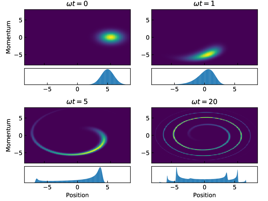
Figure 1: Diagrams of an atomic cloud as dephasing causes quasi-thermal equilibrium. The figure is separated into four parts, with the top subplot showing the phase space density of the cloud at a given time, and the bottom subplot shows the density distribution in space only. As time passes, atoms with small differences in energy lose phase coherence until the cloud eventually spreads out along the bottom of the trap, almost as if it has thermalized, even though the model contains no interactions at all.

For the remainder of the paper, we will describe the dynamics of a single particle to be

$$x(t)=\sqrt{\frac{2E}{m\omega^{2}}}\cos(\Omega t-\phi_{0}),$$ (5)

where $\tan\phi_{0}=p_{0}/m\omega x_{0}$ and

$$\frac{\Omega}{\omega}=1+\frac{3}{8}\frac{2E}{m\omega^{2}x_{4}^{2}}.$$ (6)

From these expressions, we see that any particle can be placed on a constant energy ellipse in phase space and traces out that ellipse with a frequency that depends only on energy, independent of the initial phase of the oscillation. Fig. 1 illustrates this effect by plotting the phase space distribution of a cloud in a harmonic-quartic trap at several different times.

A classical cloud of atoms can be described by its phase space density, $f(x,p,t)$, where the phase space density describes the probability density to find an atom with the position $x$ and momentum $p$ at time $t$. The n^th moment of position of a cloud of atoms is

$$\langle x^{n}\rangle=\int_{-\infty}^{\infty}\int_{-\infty}^{\infty}dxdp\,x^{n}f(x,p,t).$$ (7)

In general, the phase space density $f(x,p,t)$ evolves in time, but in a non-interacting system each element of phase space moves independently from all others and can be tracked as it evolves. By backtracking each point and its phase space density back to $t=0$, one can remove the dynamics from $f(x,p,t)$ and incorporate them into $x^{n}$ such that

$$\langle x^{n}\rangle=\int_{-\infty}^{\infty}\int_{-\infty}^{\infty}dxdp\,x_{R}^{n}(x,p,t)f_{0}(x,p),$$ (8)

where $x_{R}(x,p,t)$ is the backtracked position at $t=0$ that the position at $(x,p,t)$ now represents.

To simplify the integration, it is convenient to transform Eq.(8) into a polar coordinate system such that

$$x=\sqrt{2\xi}\sigma_{x}\cos\phi\>\mathrm{and}\>p=\sqrt{2\xi}\sigma_{p}\sin\phi,$$ (9)

where $\xi=E/k_{B}T$ is the ratio between phase space energy, Eq. (4), and thermal energy, where $T$ is the initial temperature of the cloud. Both coordinate and momentum are scaled by the thermal standard deviations,

$$\sigma_{p}=\sqrt{mk_{B}T}\>\mathrm{and}\>\sigma_{x}=\sqrt{k_{B}T/m\omega^{2}},$$ (10)

to make them unitless. The angle $\tan(\phi)=\sigma_{x}p/\sigma_{p}x$ is the initial polar angle of some point $(x,p)$ at $t=0$. In this new coordinate system

$$x_{R}=\sqrt{2\xi}\sigma_{x}\cos(\Omega t+\phi),$$ (11)

and Eq. (8) becomes

$$\frac{\langle x^{n}\rangle}{(\sqrt{2}\sigma_{x})^{n}}=\int_{0}^{\infty}\int_{0}^{2\pi}d\xi d\phi\sigma_{x}\sigma_{p}\xi^{n/2}\cos^{n}(\Omega t+\phi)f_{0}(\xi,\phi),$$ (12)

where $f_{0}(\xi,\phi)$ is simply the initial phase space density distribution converted to the new coordinate basis.

First consider the case where the atomic cloud is prepared in thermodynamic equilibrium at temperature $T$, in the trapping potential with frequency $\omega$. At time $t=0$ the cloud is given a kick, resulting in initial center of mass conditions

$$p_{D}=\sqrt{2\xi_{D}}\sigma_{p}\sin\phi_{D}\>\mathrm{and}\>x_{D}=\sqrt{2\xi_{D}}\sigma_{x}\cos\phi_{D}.$$ (13)

$\xi_{D}$ and $\phi_{D}$ are defined with respect to $x_{D}$ and $p_{D}$ in the same way that $\xi$ and $\phi$ are defined in terms of $x$ and $p$, such that

$$\xi_{D}=\frac{x_{D}^{2}}{2\sigma_{x}^{2}}+\frac{p_{D}^{2}}{2\sigma_{p}^{2}}\textrm{ and }\tan(\phi_{D})=\sigma_{x}p_{D}/\sigma_{p}x_{D}.$$ (14)

Starting from a thermal distribution in the harmonic trap, we displace it by $x_{D}$ and $p_{D}$, and convert to the polar coordinate system, leading to

$$f_{0}=\frac{1}{2\pi\sigma_{x}\sigma_{p}}\exp\left(-\xi-\xi_{D}+2\sqrt{\xi\xi_{D}}\cos(\phi-\phi_{D})\right).$$ (15)

Substituting Eq. (15) into Eq. (12) and converting the integral to the new variables yields

$$\frac{\langle x^{n}\rangle}{(\sqrt{2}\sigma_{x})^{n}}=\frac{e^{-\xi_{D}}}{2\pi}\int_{0}^{\infty}d\xi\xi^{n/2}e^{-\xi}\int_{0}^{2\pi}d\phi\cos^{n}(\Omega t+\phi_{D}+\phi)\exp\left(2\sqrt{\xi\xi_{D}}\cos\phi\right).$$ (16)

The trigonometric power law reduction formula, $\cos^{n}\theta=\sum_{m}c_{nm}\cos m\theta$, permits further simplification. Analytic expressions for the coefficients $c_{nm}$ can be found in Gradshteyn and Ryzhik (2007), on page 31. In this case, the three elements of interest are $c_{11}=1$, $c_{20}=1/2$, and $c_{22}=1/2$.

Perhaps surprisingly, Equation (16) can be solved analytically without further approximation. To simplify the notation, the moments can be rewritten as

$$\frac{\langle x^{n}\rangle}{(\sqrt{2}\sigma_{x})^{n}}=\frac{1}{2}\sum_{m}c_{nm}\left({\Upsilon}_{nm}+c.c\right),$$ (17)

with the $\Upsilon_{nm}$ given as

$${\Upsilon}_{nm}=e^{-\xi_{D}+im(\omega t+\phi_{D})}\int_{0}^{\infty}d\xi\xi^{n/2}\exp\left[-\left(1-im\Lambda t\right)\xi\right]I_{m}(2\sqrt{\xi\xi_{D}}),$$ (18)

where $\Lambda\equiv 3\omega\sigma_{x}^{2}/8x_{4}^{2}$ and $I_{m}$ is the modified Bessel function of the first kind. The integrals in $\Upsilon_{20}$, $\Upsilon_{11}$ and $\Upsilon_{22}$ must be solved to calculate closed-form expressions for $\langle x\rangle$ and $\langle x^{2}\rangle$. The integrals in $\Upsilon_{11}$ and $\Upsilon_{22}$ can be solved in terms of Gradshteyn and Ryzhik (2007), section 6.631, equation 4. $\Upsilon_{20}$ can be solved in terms of equation 1 in the same section. The results are

$$\Upsilon_{20}=1+\xi_{D},$$ (19)

$$\Upsilon_{11}=\frac{\sqrt{\xi_{D}}}{(1-i\Lambda t)^{2}}\exp\left[-\xi_{D}+\frac{\xi_{D}}{(1-i\Lambda t)}+i(\omega t+\phi_{D})\right],$$ (20)

and

$$\Upsilon_{22}=\frac{\xi_{D}}{(1-2i\Lambda t)^{3}}\exp\left[-\xi_{D}+\frac{\xi_{D}}{(1-2i\Lambda t)}+i(2\omega t+2\phi_{D})\right].$$ (21)

With these solutions, it is possible to calculate the center-of-mass position and size of the cloud as a function of time for any chosen set of parameters that satisfies the requirement that the initial kick produce a maximum displacement in position much less than $|x_{4}|$.

III Results

Having calculated the values of $\Upsilon_{nm}$, we can combine them into expressions for physical properties that can be easily measured in an experimental realization of this system. The center-of-mass position and size of the cloud are, in general, easily observed and calculated from absorption images.

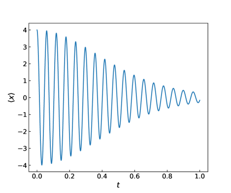
Figure 2: $\langle x\rangle$ as a function of time. Most of the decay to quasi-thermal equilibrium is shown. The plot uses parameters $\xi_{D}=8$, $\phi_{D}=0$, $\omega=100$, $\sigma_{x}(t=0)=1$, and $x_{4}=8$. For these parameters, $\Lambda\cong 0.586$.

$\Upsilon_{11}$ leads to the center-of-mass position of the atomic cloud as a function of time.

$$\langle x\rangle=\frac{\sigma_{x}\sqrt{2\xi_{D}}}{[1+(\Lambda t)^{2}]^{2}}\exp\left[\frac{-(\Lambda t)^{2}\xi_{D}}{1+(\Lambda t)^{2}}\right]\left(\cos(\Phi_{1})-2\Lambda t\sin(\Phi_{1})-(\Lambda t)^{2}\cos(\Phi_{1})\right),$$ (22)

where $\Phi_{1}=\omega t+\phi_{D}+\Lambda t\xi_{D}/(1+(\Lambda t)^{2})$. The first moment resembles a decaying sinusoid. The initial decay is Gaussian, but at later times the denominator of the first term takes over. $\Upsilon_{20}$ and $\Upsilon_{22}$ combine to give the second moment

$$\langle x^{2}\rangle=\sigma_{x}^{2}(1+\xi_{D})+ \frac{\sigma_{x}^{2}\xi_{D}}{[1+(2\Lambda t)^{2}]^{3}}\exp\left[\frac{-(2\Lambda t)^{2}\xi_{D}}{1+(2\Lambda t)^{2}}\right]$$ (23)

$$\times\left(\cos(\Phi_{2})-6\Lambda t\sin(\Phi_{2})-12(\Lambda t)^{2}\cos(\Phi_{2})+8(\Lambda t)^{3}\sin(\Phi_{2})\right),$$

where $\Phi_{2}=2\omega t+2\phi_{D}+2\Lambda t\xi_{D}/(1+(2\Lambda t)^{2})$. This has a similar form to $\langle x\rangle$, but it oscillates about twice as rapidly, and decays faster as well, as seen in Figure 3. In fact, the second moment is less illustrative of the dynamics than the size of the cloud as a function of time because the position and size of the cloud are more directly measurable. The standard deviation of the cloud’s position distribution, hereafter referred to as the “cloud size” is $\sigma(t)=\sqrt{\langle x^{2}\rangle-\langle x\rangle^{2}}$ and an example is shown in Figure 4. The decay rates are important indicators of the harmonicity of the trap, and in an experimental realization, adjusting the trap parameters to minimize the decay rate leads toward a maximally harmonic trap.

There is an alternative formulation for the first two moments that works for $\Lambda t\ll 1$ and converts the oscillatory part into a single cosine. For the first moment, the approximation yields

$$\langle x\rangle=\frac{\sqrt{2\xi_{D}}\sigma_{x}}{(1+(\Lambda t)^{2})^{2}}\mathrm{exp}\left[\frac{-(\Lambda t)^{2}\xi_{D}}{1+(\Lambda t)^{2}}\right]\cos\left(\omega t+\phi_{D}+2\Lambda t+\frac{\Lambda t\xi_{D}}{1+(\Lambda t)^{2}}\right).$$ (24)

Of particular note is the argument of the cosine. The usual $\omega t+\phi_{D}$ is present, and there is a term proportional to $\xi_{D}$, representing the frequency dependence on the strength of the initial sloshing, but the $2\Lambda t$ term is independent of the kick strength. In other words, the frequency of oscillation for a cloud is different from that of a single particle, with a frequency difference that tends to a nonzero value even as the oscillation amplitude approaches zero. Contrast this with Equation 5, where the value of $\Omega$ for a single particle approaches $\omega$ as the amplitude tends to zero.

Figure 2 shows an example of this solution for a set of parameters chosen to showcase the behavior of the cloud as it approaches quasi-thermal equilibrium. The center-of-mass oscillations gradually decay, and eventually no center-of-mass oscillations will be observed. As discussed previously, this model does not take collisions into account, so the apparent thermalization is purely a result of the relative dephasing of parts of the cloud with different energies.

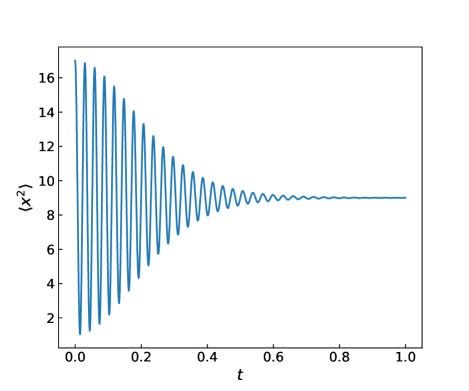
Figure 3: $\langle x^{2}\rangle$ as a function of time for the same parameters as used in Figure 2. Note the more rapid oscillations as well as the more rapid decay of the oscillations.

Next, the same approximation applied to $\Upsilon_{22}$ leads to an approximate expression for the second moment of position.

$$\langle x^{2}\rangle=\sigma_{x}^{2}(1+\xi_{D})+ \frac{\sigma_{x}^{2}\xi_{D}}{(1+(2\Lambda t)^{2})^{3}}\mathrm{exp}\left[\frac{-(2\Lambda t)^{2}\xi_{D}}{1+(2\Lambda t)^{2}}\right]$$ (25)

$$\times\cos\left[2\omega t+2\phi_{D}+6\Lambda t+\frac{2\Lambda t\xi_{D}}{1+(2\Lambda t)^{2}}\right].$$

These two moments can similarly be combined to approximate the cloud size as a function of time.

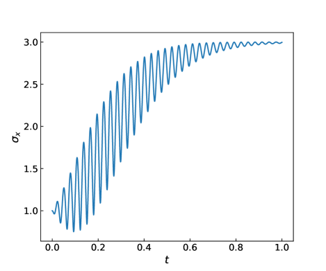
Figure 4: The size of the cloud as a function of time, using the same parameters as Figures 2 and 3.

IV Time of Flight

In an experimental setting, it is likely that the atomic clouds will be imaged after a period of free-fall, in order to increase the size of the cloud and its observed oscillation amplitude. Limited analytical understanding of the behavior of the clouds after time-of-flight is possible, but numerical calculations can more easily illuminate these effects.

The effect on the first moment is a change in amplitude and a phase shift that depends on the time of flight. Looking at the form of the first moment, Equation (22), its general behavior is that of a sinusoid with a slowly varying amplitude. This functional form is approximated by

$$\langle x\rangle\approx M(t)\cos(\Omega t+\phi_{1}),$$ (26)

where $M(t)$ is the decay function, $\Omega$ represents the real oscillation frequency of the cloud, and $\phi_{1}$ represents some initial phase.

Taking the derivative of this expression, assuming that the variation of $M(t)$ is slow compared to the sinusoid, results in

$$\frac{\partial\langle x\rangle}{\partial t}\approx-\Omega M(t)\sin(\Omega t+\phi_{1}),$$ (27)

which has the same frequency of oscillation and a similar decay rate, insofar as the variation of $M(t)$ is slow, to the dynamics without time of flight. Assuming the $x$ axis is perpendicular to gravity, the horizontal velocity of the cloud is constant after the trap is released. The result is an expression that oscillates at the same frequency as in the trap, but with a different phase and amplitude that depend on the time of release and the elapsed time of flight.

The behavior of the cloud size requires more careful consideration. Since the cloud is oscillating in a potential much larger than the cloud, the cloud may experience dispersion which can cause the cloud to expand more or less quickly after the trap is released, depending on the phase of the oscillation at the time of release. This complication makes writing an analytical solution, even a highly approximate one, to $\sigma$ after free-fall much more difficult.

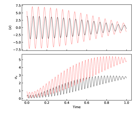
Figure 5: Pictured here are the results of a simple Monte-Carlo numerical simulation of sloshing in a harmonic/quartic trap, with trapping parameters similar to those used in earlier figures. Fourth-order Runge-Kutta integration was used to evolve the system. The black curves represent the position and size of the cloud without taking time of flight into account. The dotted curves (red online) the position and size of the cloud after a short time of flight (0.015). The time of flight exaggerates the oscillations in $\sigma_{x}$, changing the shape of the curve.

Figure 5 shows the results of a numerical model which shows the behavior of $\langle x\rangle$ and $\sigma$, in conditions chosen to be similar to the parameters used in Figures (2), (3), and (4). We observe that the behavior with and without time of flight are similar but the time of flight data has a larger amplitude of oscillation, a larger cloud size in general, and a slightly different size profile as time goes on, with more exaggerated size oscillations in the middle times.

V Conclusions and Outlook

The oscillations along the weak axis of a small cloud in a perfectly harmonic cigar-shaped trap are not expected to decay significantly over time, based on a straightforward extension of the calculations in Guéry-Odelin et al. (1999). The addition of non-harmonic terms causes the cloud to gradually spread out and reach quasi-thermal equilibrium even without interactions, as atoms with different energies gradually dephase.

Our analytical model describes the dynamics of a cloud of neutral atoms in a harmonic trap with a quartic perturbation. We assume that the displacement of the cloud is less than the magnitude of the quartic parameter $x_{4}$, that mean-field effects are negligible, that collisions are isotropic, elastic, and energy-independent, and that the quartic contribution does not significantly affect the magnitude of the collisional integral.

With a few minor approximations, the system is analytically solvable. The analytical expressions can be used as fitting functions for the observed behavior of ensembles of cold atoms in a nearly- harmonic trap. The motion of the ensemble’s center of mass and the evolution of its size permit easy determination of trap anharmonicity, and given the right trap architecture, the anharmonic parts can be tuned to some desired value. Time-of-flight imaging makes small changes to the observed values of the variables but does not qualitatively change the behavior of the ensemble. Thus, even with time-of-flight imaging, the fit parameters for the trap will still maintain the same relative trends.

The construction of a trap geometry which can control various polynomial terms while minimizing unwanted terms is discussed in Stickney et al. (2014). The specific calculations for a trap allowing adjustment of harmonic and quartic terms, while canceling polynomial terms out to sixth order are also detailed there. Dynamic control of the shape of the trap is expected to produce additional interesting results. For instance, because the equilibrium is not a true thermal equilibrium, it should be possible to dephase and rephase the cloud as it oscillates as long as the collision rate is not too high, and effective “pauses” in the dephasing of the cloud might be made possible by turning off the quartic contributions. These qualities make the dynamically controlled trap an interesting topic worthy of experimental examination.

VI Acknowledgments

This work was funded by the Air Force Research Laboratory.

References

- Fixler et al. (2007) J. B. Fixler, G. T. Foster, J. M. McGuirk, and M. A. Kasevich, Science 315, 74 (2007).
- Peters, Chung, and Chu (2001) A. Peters, K. Y. Chung, and S. Chu, Metrologia 38, 25 (2001).
- Bertoldi et al. (2006) A. Bertoldi, G. Lamporesi, L. Cacciapuoti, M. de Angelis, M. Fattori, T. Petelski, A. Peters, M. Prevedelli, J. Stuhler, and G. M. Tino, Eur. Phys. J. D 40, 271 (2006).
- Canuel et al. (2006) B. Canuel, F. Leduc, D. Holleville, A. Gauguet, J. Fils, A. Virdis, A. Clairon, N. Dimarcq, C. J. Bordé, A. Landragin, and P. Bouyer, Phys. Rev. Lett. 97, 010402 (2006).
- Wu et al. (2017) X. Wu, F. Zi, J. Dudley, R. J. Bilotta, P. Canoza, and H. Müller, Optica 4, 1545 (2017).
- Dickerson et al. (2013) S. M. Dickerson, J. M. Hogan, A. Sugarbaker, D. M. Johnson, and M. A. Kasevich, Phys. Rev. Lett. 111, 083001 (2013).
- Burke and Sackett (2009) J. H. Burke and C. A. Sackett, Phys. Rev. A 80, 061603(R) (2009).
- Wu, Su, and Prentiss (2007) S. Wu, E. J. Su, and M. G. Prentiss, Phys. Rev. Lett. 99, 173201 (2007).
- Dutta et al. (2016) I. Dutta, D. Savoie, B. Fang, B. Venon, C. L. Garrido Alzar, R. Geiger, and A. Landragin, Phys. Rev. Lett. 116, 183003 (2016).
- Deissler et al. (2008) B. Deissler, K. J. Hughes, J. H. T. Burke, and C. A. Sackett, Phys. Rev. A 77, 031604(R) (2008).
- Bouchendira et al. (2011) R. Bouchendira, P. Cladé, S. Guellati-Khélifa, F. Nez, and F. Biraben, Phys. Rev. Lett. 106, 080801 (2011).
- Chung et al. (2009) K. Y. Chung, S. W. Chiow, S. Herrmann, S. Chu, and H. Müller, Phys. Rev. D 80, 016002 (2009).
- Horikoshi and Nakagawa (2007) M. Horikoshi and K. Nakagawa, Phys. Rev. Lett. 99, 180401 (2007).
- Stickney et al. (2014) J. A. Stickney, B. Kasch, E. Imhof, B. R. Kroese, J. A. R. Crow, S. E. Olson, and M. B. Squires, Phys. Rev. A , 053606 (2014).
- Guéry-Odelin et al. (1999) D. Guéry-Odelin, F. Zambelli, J. Dalibard, and S. Stringari, Phys. Rev. A 60, 4851 (1999).
- Lobser et al. (2015) D. S. Lobser, A. E. S. Barentine, E. A. Cornell, and H. J. Lewandowski, Nature Physics 11, 1009 (2015).
- Gradshteyn and Ryzhik (2007) I. S. Gradshteyn and I. M. Ryzhik, Table of integrals, series, and products, 7th ed. (Elsevier/Academic Press, Amsterdam, 2007) translated from the Russian, Translation edited and with a preface by Alan Jeffrey and Daniel Zwillinger.